


1. Introduction
1.1 Differentiation, lambda-calculus and linear logic
Linear logic (LL) is a logical system that arose from semantics (Girard (Reference Girard1987)), following the observation that some interesting models of the
 $\lambda$
-calculus were actually the coKleisli category
 $\mathscr {L}_{{!}}$
of some category
 $\mathscr {L}$
of linear morphisms. That is, a morphism from object
 $X$
to
 $Y$
can be seen as a morphism in
 $\mathscr {L}(!X, Y)$
, where
 $\mathscr {L}\,$
is a category of linear morphisms and
 $!\_$
is a comonad on
 $\mathscr {L}$
. The syntactical counterpart of a morphism in
 $\mathscr {L}$
is a proof/program that uses its input (data or hypothesis) exactly once, and the syntactical version of
 $!\_$
features a construction (called promotion) that makes a resource duplicable and discardable.
It turns out that in multiple models of LL, the morphisms
 $f \in \mathscr {L}(!X, Y)$
are differentiable in some sense, strongly suggesting that differentiation of proofs and programs should be considered as a natural LL operation. Remember (see Dieudonné (Reference Dieudonné1969) for instance) that for any Banach spaces
 $E$
and
 $F$
, a function
 $f:E\to F$
is differentiable at
 $x \in E$
if there is a neighborhood
 $U$
of
 $0$
in
 $E$
and a linear and continuous function
 $\varphi :E\to F$
such that, for all
 $u\in U$
 \begin{align} f(x+u)=f(x)+\varphi (u)+o(\|u\|)\,. \end{align}
When
 $\varphi$
exists, it is unique and is denoted as
 $f'(x)$
. When
 $f'(x)$
exists for all
 $x\in E$
, the function
 $f' :E\to \mathscr {L}(E,F)$
, where
 $\mathscr {L}(E,F)$
is the Banach space of linear and continuous functions
 $E\to F$
, is called the differential of
 $f$
. This function can itself admit a differential and so on. When all these iterated differentials exist one says that
 $f$
is smooth and the
 $n$
th derivative of
 $f$
is a function
 $f^{( )}n :E\to \mathscr {L}_n(E,F)$
where
 $\mathscr {L}_n(E,F)$
is the space of continuous
 $n$
-linear symmetric functions
 $E^n\to F$
. It can even happen that
 $f$
is locally (or even globally) expressed using its iterated derivatives by means of the Taylor Formula,
 \begin{equation} f(x+u)=\sum _{n=0}^\infty \frac 1{n!} f^{(n)}(x) (u,\dots, u). \end{equation}
When this holds locally at any point
 $x$
,
 $f$
is said to be analytic, see Whittlesey (Reference Whittlesey1965).
Based on categorical models of LL where objects are similar to vector spaces and morphisms
 $f \in \mathscr {L}(!X, Y)$
are analytic functions from
 $X$
to
 $Y$
, the differential
 $\lambda$
-calculus (Ehrhard and Regnier (Reference Ehrhard and Regnier2003)) and differential LL provide a logical and syntactical account of differentiation. If
 $\Gamma, x : A \vdash P : B$
and
 $\Gamma \vdash Q : A$
, then one can define in these systems, by purely syntactical means, a program
 $\Gamma, x : A \vdash \frac {\partial P}{\partial x} \cdot Q : B$
whose denotational semantics in such models is the derivative of the interpretation of
 $P$
wrt. the variable
 $x$
, linearly applied to the semantics of
 $Q$
. This syntactic derivative can be seen as a version of
 $P$
, where exactly one call to the variable
 $x$
that occurs during the computation of
 $P$
is replaced with a call to
 $Q$
: this explains why
 $x$
is still free in
 $\frac {\partial P}{\partial x} \cdot Q$
in general. This provides a new approach of finite approximations of programs by a syntactical version of the Taylor Formula whose effect is to translate
 $\lambda$
-calculus application
 $(P)Q$
into the differential
 $\lambda$
-calculus in such a way that
 \begin{equation} (\lambda x. P)Q \text { reduces to } \sum _{n=0}^{\infty } \frac {1}{n!} \left ( \frac {\partial ^n P}{\partial x^n} (\underbrace {Q, \ldots, Q}_{\text {n times}}) \right ) [0/x]\,. \end{equation}
The term of rank
 $n$
in this formal sum corresponds to the part of the computation that uses the input
 $Q$
exactly
 $n$
times. Applying this transformation hereditarily to all the applications occurring in a
 $\lambda$
-term, it becomes possible to turn it into an infinite sum of strongly normalizing resource terms, see Ehrhard and Regnier (Reference Ehrhard and Regnier2008).
Differentiation is deeply connected with addition, as it can already be seen in its definition Eq. (1) and in the syntactical Taylor expansion Eq. (3). As a result, the differential
 $\lambda$
-calculus is always endowed with an unrestricted operation of sum between terms. Similarly, all categorical models of the differential
 $\lambda$
-calculus and of differential LL (see Reference Blute, Cockett and SeelyBlute et al., (2006, 2009)) were using categories where the hom-sets were commutative monoids, and all models of the syntactical Taylor expansion (Manzonetto (Reference Manzonetto2012)) require the hom-sets to feature arbitrary countable sums. The only available operational interpretation of such a sum being erratic choice, these formalisms are inherently non-deterministic. This is in sharp contrast with the uniformity property of the sum that can be observed in the syntax. For example, if the term of Eq. (3) reduces to a variable, then only one term of the sum is non-zero. The position
 $n$
of this term gives the number of times the term
 $Q$
is evaluated during the weak head reduction strategy as shown in Ehrhard and Regnier (Reference Ehrhard and Regnier2003). Furthermore, many deterministic (or probabilistic) models of LL such as those based on the relational model (like coherence spaces and probabilistic coherent spaces) feature morphisms in
 $\mathscr {L}(!X, Y)$
, which are clearly analytic in some sense, although the hom-sets do not feature a commutative monoid structure.
1.2 Coherent differentiation
Recently, Ehrhard (Reference Ehrhard2022) observed that, in a setting where all coefficients are non-negative, differentiation survives to strong restrictions on the use of addition. Consider for instance a function
 $[0,1]\to [0,1]$
which is smooth on
 $[0,1)$
and all of whose iterated derivatives are everywhere
 $\geq 0$
.Footnote 1 If
 $x,u\in [0,1]$
are such that
 $x+u\in [0,1]$
then
 \begin{equation} f(x)+f'(x)u\leq f(x+u)\in [0,1]. \end{equation}
This makes sense even if
 $f'(1)=\infty$
, which can happen: take
 $f(x)=1-\sqrt {1-x}$
. So if
 $S$
is the set of all such pairs
 $\left \langle \!\left \langle x, u \right \rangle \!\right \rangle$
that we call summable, we can consider the function
 \begin{equation*} \widetilde {\mathsf {D}}(f) : \left \langle \!\left \langle x, u \right \rangle \!\right \rangle \mapsto \left \langle \!\left \langle f(x), f'(x) \cdot u \right \rangle \!\right \rangle \end{equation*}
as a map
 $S\to S$
. This basic observation is generalized in Ehrhard (Reference Ehrhard2023b) to a wide range of categorical models
 $\mathscr {L}$
of LL including coherence spaces, probabilistic coherence spaces, etc. where hom-sets have only a partially defined addition. In these summable categories, we obtain an endofunctor
 $\mathsf {S} : \mathscr {L}\to \mathscr {L}$
equipped with an additional structure which allows defining summability and (partial) finite sums in a very general way that turns
 $\mathsf {S}$
into a monad. Differentiation is then axiomatized as a distributive law
 $! \mathsf {S} \Rightarrow \mathsf {S} !$
between this monad (similar to the tangent bundle monad of a tangent category, see Rosicky (Reference Rosicky1984)) and the resource comonad
 $!\_$
of the LL structure of the categoryFootnote 2
 $\mathscr {L}$
. Indeed, this distributive law allows one to extend
 $\mathsf {S}$
to
 $\mathscr {L}_{{!}}$
, the coKleisli category of
 $!\_$
, and this extension
 $\widetilde {\mathsf {D}}:\mathscr {L}_{{!}} \to \mathscr {L}_{{!}}$
inherits the monad structure of
 $\mathsf {S}$
. A category equipped with such a differentiation is then called a coherent differential category. It was also observed that the functor
 $\mathsf {S}$
is often representable, following the terminology of tangent categories (see Cockett and Cruttwell (Reference Cockett and Cruttwell2014)), meaning that
 $\mathsf {S} = \mathbb {D} \multimap \_$
(the category
 $\mathscr {L}$
being most often symmetric monoidal closed, with internal hom of
 $X$
and
 $Y$
denoted as
 $X\multimap Y$
), where
 $\mathbb {D} = 1{} \& 1{}$
(
 $1{}$
is the unit of the tensor product of
 $\mathscr {L}$
, and
 $\&$
is a cartesian product). This object
 $\mathbb {D}$
can be endowed with the structure of a comonoid from which the monad structure of
 $\mathsf {S}$
arise. Differentiation then boils down to the existence of a coalgebra structure
 $\mathbb {D} \rightarrow ! \mathbb {D}$
on
 $\mathbb {D}$
which is compatible with its comonoid structure.
1.3 Contributions of this work
The goal of the present article is to study the Taylor expansion in this setting of partial sums. We believe that this is a crucial step toward providing generic tools to define a denotational semantics of the differential
 $\lambda$
-calculus and of the syntactical Taylor expansion in a much more general setting than the current state of the art of Manzonetto (Reference Manzonetto2012). The starting idea is that for the same reason that
 $\widetilde {\mathsf {D}} f(x) = \left \langle \!\left \langle f(x), f'(x) u \right \rangle \!\right \rangle$
is defined, it should be possible to define directly a second order approximant.
 \begin{equation*}\mathsf {T} f \left \langle \!\left \langle x, u_1, u_2 \right \rangle \!\right \rangle = \left \langle \!\left \langle f(x), f'(x) \cdot u_1, {\frac {1}{2} f^{(2)}(x) \cdot (u_1, u_1) + f'(x) \cdot u_2 }\right \rangle \!\right \rangle. \end{equation*}
The term
 $u_1$
should be seen as a first-order variation and the term
 $u_2$
as a second-order variation. So
 $\mathsf {T} f \left \langle \!\left \langle x, u_1, u_2 \right \rangle \!\right \rangle$
gives the components (sorted by order) of the order 2 Taylor approximation of
 $f$
on the variation
 $u_1 + u_2$
. Similarly to Eq. (4), this sum is lower than
 $f(x+u_1+u_2)$
, so it is well-defined. This idea should work for any order, and going to the limit, for an infinite amount of coefficient, yielding an operator which provides all the terms of the Taylor expansion.
The first step is to introduce the
 $\Sigma$
-summabibility structure
 $\mathsf {S}$
, an infinitary counterpart of the summability structure previously mentioned. This
 $\Sigma$
-summability structure is infinitary in the sense that an “element” of
 $\mathsf {S}(X)$
is a
 $\mathbb {N}$
-indexed family of elements of
 $X$
whose infinitary sum is well-defined, the underlying notion of infinitary sum is the one of
 $\Sigma$
-monoid, see Haghverdi (Reference Haghverdi2000). It turns out that
 $\mathsf {S}$
is not only a monad but also a comonad. The monadic and comonadic structures interact well, turning
 $\mathsf {S}$
into a bimonad (section 4). Surprisingly, the whole Taylor expansion operation is again a distributive law
 $! \mathsf {S} \Rightarrow \mathsf {S} !$
following the exact same properties as coherent differentiation. This distributive law allows, as it is standard, to extend the functor
 $\mathsf {S}$
into a functor
 $\mathsf {T}:\mathscr {L}_{!}\to \mathscr {L}_{!}$
which implements Taylor expansion and inherits the monadic structure of
 $\mathsf {S}$
. One more axiom is added, ensuring intuitively that the maps are analytic in the sense that they coincide with their Taylor expansion. This axiom was the missing piece to ensure that
 $\mathsf {T}$
inherits from
 $\mathsf {S}$
the structure of a bimonad. We call a category equipped with such Taylor expansion an analytic category (section 6).
Similarly to coherent differentiation, in many concrete models of LL, the functor
 $\mathsf {S}$
is representable and is equal to
 $\mathbb {D} \multimap \_$
where this time
 $\mathbb {D} = 1{} \& 1{} \& \cdots$
(
 $\mathbb {N}$
-indexed cartesian product). A category is called representably
 $\Sigma$
-additive if this functor
 $\mathsf {S}$
is a
 $\Sigma$
-summability structure. This object
 $\mathbb {D}$
can be endowed with the structure of a bimonoid that completely determines the bimonad structure of
 $\mathsf {S}$
. The analytic Taylor expansion — that is, the aforementioned distributive law
 $! \mathsf {S} \Rightarrow \mathsf {S} !$
— then boils down to a coalgebra
 $\mathbb {D} \rightarrow ! \mathbb {D}$
compatible with the bimonoid structure (section 9). We call representably analytic categories such instance of analytic categories. This coalgebra structure always exist when the exponential (the
 $!\_$
comonad) is free, that is, when the category is Lafont, Lafont (Reference Lafont1988). This implies the following result.
Theorem 1.
Any representably
 $\Sigma$
-additive Lafont category is a representably analytic category.
We provide many examples of representably analytic Lafont categories. First, we discuss in section 10 that the relational model and the weighted relational model are Lafont representably analytic categories. We compute explicitly the action of the
 $\mathsf {T}$
functor on morphisms, showing that
 $\mathsf {T}$
performs the expected Taylor expansion. It means that our theory of analytic category covers the most important models of differential LL and of syntactical Taylor expansion, so and should be a strict generalization of the theory of Manzonetto (Reference Manzonetto2012).
Then, we provide many examples which were not captured by this previous theory. The first example is based on a notion of coherence space introduced in Lamarche (Reference Lamarche, Brookes, Main, Melton and Mislove1995), which seems deeply related to Scott semantics. The second one is based on nonuniform coherence spaces that were introduced in Bucciarelli and Ehrhard (Reference Bucciarelli and Ehrhard2001) and are known to have two different exponentials, one of them being the free exponential. In this setting, the free exponential provides an example of representably analytic category, but we show that the non-free one is not a representably analytic category, yet is a representably coherent differential category in the sense of Ehrhard (Reference Ehrhard2023b). We also mention the fact that the usual Girard’s coherence spaces, with their free exponential, are a representably analytic category, and last we deal with the case of probabilistic coherence spaces (introduced in Danos and Ehrhard (Reference Danos and Ehrhard2011a)) whose only known exponential has been shown to be free. They provide yet another example of representably analytic category where morphisms are analytic functions with non-negative real coefficients.
1.4 Taylor expansion in cartesian closed categories.
Because
 $\mathscr {L}_{{!}}$
is a cartesian closed category, it can be interesting to drift away from the structure of
 $\mathscr {L}$
by only looking at the structure induced in
 $\mathscr {L}_{{!}}$
. This is what happened with differentiation. It was first categorically axiomatized in a typical LL setting with additive categories, introducing a notion of differential categories in Blute et al. (Reference Blute, Cockett and Seely2006). Differentiation was then carried to the setting of cartesian left-additive categories, introducing cartesian differential categories in Blute et al. (Reference Blute, Cockett and Seely2009), leading to successful uses of differentiation outside the realm of LL. Unsurprisingly, the coKleisli categories of differential LL categories are instances of cartesian differential categories, but the latter are more general than the former and cover more examples of categories where differentiation is available. Similarly, left summability structures and cartesian coherent differential categories were introduced in Ehrhard and Walch (Reference Ehrhard and Walch2023) to axiomatize coherent differentiation directly in any cartesian category. They arise in particular as the coKleisli category of coherent differential categories, and are at the same time a conservative generalization of the cartesian differential categories.
Since analytic categories are very similar to coherent differential categories, it is possible to introduce in a very similar way a notion of cartesian analytic category (section 7). We can then define the notion of a cartesian closed analytic category. This more direct axiomatization should provide the foundation for working on the denotational semantics of syntactical Taylor expansion, but also provide a categorical framework for Taylor expansion independent of LL.
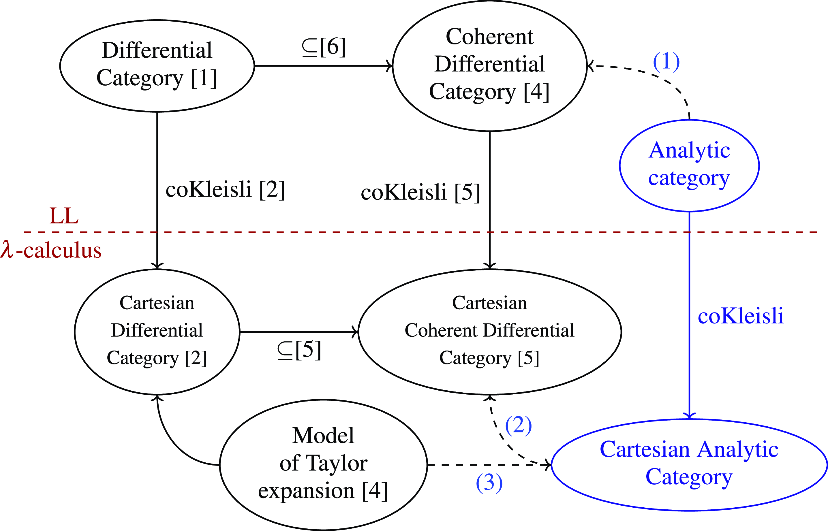
Map of concepts, [1] Blute et al. (Reference Blute, Cockett and Seely2006) [2] Blute et al. (Reference Blute, Cockett and Seely2009) [3] Manzonetto (Reference Manzonetto2012) [4] Ehrhard (Reference Ehrhard2023b) [5] Ehrhard and Walch (Reference Ehrhard and Walch2023) [6] Walch (Reference Walch2022).

1.5 Map of concepts
We summarize in Figure 1 how the different concepts relate with each other. We expect the dashed arrows to hold, but the proofs are postponed to further work.
The arrows (1) and (2) should be a consequence of the fact that the Taylor functor performs Taylor expansion at all order, and in particular includes Taylor expansion at order one, which yield precisely the definition of the derivative in Eq. (1). The reverse arrow does not hold, a coherent differential category is not always an analytic category, we provide such example in Section 11.3.
We expect the arrow (3) to hold because our notion of analytic categories cover both the relational model and the weighted relational model, and the Taylor functor performs the expected Taylor expansion, as discussed in section 10. These two models are the two principal models of syntactical Taylor expansion following the definition of Manzonetto (Reference Manzonetto2012), so our new theory captures the main examples of the previous theory.
1.6 Mates and distributive law
One contribution of this article is to exhibit the crucial role played by the mate construction (section 8) in the representable case, both in the setting of Ehrhard (Reference Ehrhard2023b) and in the setting of this article. In the representable case, the commutative bimonoid
 $\mathbb {D}$
induces a bimonad
 $\_ \otimes \mathbb {D}$
. This bimonad is the left adjoint of
 $\mathsf {S} = \mathbb {D} \multimap \_$
, so the mate construction induces a bimonad structure on
 $\mathsf {S}$
that turns out to be precisely the one described in Section 4.4. Then the mate construction also induces a bijection between natural transformations
 $\partial : !\mathsf {S} \Rightarrow \mathsf {S} !$
and
 $\overline {\partial } : (! \_ \otimes \mathbb {D}) \Rightarrow ! (\_ \otimes \mathbb {D})$
, and it turns out that this bijection preserves distributive laws. It provides a crucial step when showing that Taylor expansion boils down to a coalgebra on
 $\mathbb {D}$
.
1.7 Related work
There might be connections between the work presented here and the recent article Kerjean and Lemay (Reference Kerjean and Lemay2023) where an account of Taylor expansion in differential LL is provided, based on the use of a resource exponential modality
 $!\_$
which has not only its standard comonad structure but also a monad structure. The article conjectures that this monad structure is compatible with the comonadic structure of
 $!\_$
, turning
 $!\_$
into a bimonad. In our setting, this is not the exponential modality which features a bimonad structure, but the infinitary summability functor
 $\mathsf {S}$
which does not at all play the same role: for instance, in LL models, the functor
 $\mathsf {S}$
preserves cartesian products whereas the
 $!\_$
functor turns the cartesian product into a tensor product. Another difference between the two approaches is that, being based on differential LL, Kerjean and Lemay (Reference Kerjean and Lemay2023) is based on additive categories whereas one of our main motivations is to deal with Taylor expansion in settings where addition is only partially defined. A more detailed analysis of the possible connections between the two approaches is definitely necessary.
The first two sections of this article consist of reminders on distributive law and monoidal monads. We encourage the reader familiar with those notions to skip these sections, and only refer to them when necessary.
2. Background: Distributive Laws
In this section, we review the well-known notion of distributive laws first introduced in Beck (Reference Beck and Eckmann1969). Distributive laws provide a solution to the following problem: given a (co)monad on a category
 $\mathscr {C}$
and some structure on
 $\mathscr {C}$
, is it possible to extend that structure to the (co)Kleisli category of that (co)monad? Dually, is it possible to lift that structure to the (co)Eilenberg-Moore category of that (co)monad?
This categorical background will be important for this paper, since coherent differentiation and Taylor expansion are both formalized by such a distributive law, allowing to extend a monad
 $\mathsf {S}$
encoding partial summability to a monad
 $\mathsf {T}$
on the coKleisli of the exponential comonad
 $!\_$
, see section 6.
This theory was mainly developed in Street (Reference Street1972) in a general
 $2$
-categorical setting (see Maranda (Reference Maranda1965) for a definition of a
 $2$
-category). We will refer to Power and Watanabe (Reference Power and Watanabe2002) as it is a more accessible introduction. For accessibility reason, we only unfold the notion in the special case of the
 $2$
-category
 $\mathbf {Cat}$
, whose objects are the (small) categories, whose morphisms are functors and whose
 $2$
-morphisms are natural transformations.
2.1 Distributive laws for monads and extension to Kleisli categories
If
 $\underline {M} = (M, \eta, \mu )$
is a monad on
 $\mathscr {C}$
, then its Kleisli category
 $\mathscr {C}_{\underline {M}}$
is the category with the same objects as
 $\mathscr {C}$
and such that
 $\mathscr {C}_{\underline {M}}(X, Y) = \mathscr {C}(X, M Y)$
. The identity is given by
 $\eta _X \in \mathscr {C}_{\underline {M}}(X, X)$
and the composition of
 $f \in \mathscr {C}_{\underline {M}}(X, Y)$
with
 $g \in \mathscr {C}_{\underline {M}}(Y, Z)$
is defined as
 \begin{equation} g \circ _{\underline {M}} f = \mu _Y \circ M g \circ f. \end{equation}
There is a functor
 $K_{\underline {M}} : \mathscr {C} \rightarrow \mathscr {C}_{\underline {M}}$
such that
 $K_{\underline {M}} X = X$
and for any
 $f \in \mathscr {C}(X, Y)$
,
 $K_{\underline {M}} f = \eta \circ f \in \mathscr {C}_{\underline {M}}(X, Y)$
. Then for any
 $f \in \mathscr {C}_{\underline {M}}(X', X)$
,
 $h \in \mathscr {C}(X, Y)$
and
 $g \in \mathscr {C}_{\underline {M}}(Y, Y')$
,
 \begin{equation} K_{\underline {M}} h \circ _{\underline {M}} f = M h \circ f \quad \quad g \circ _{\underline {M}} K_{\underline {M}} h = g \circ h. \end{equation}
These equations are obtained by a straightforward computation using naturality and the triangle identities of the monad.
Throughout this section, we assume that
 $\underline {M}_1 = (M_1, \eta _1, \mu _1)$
is a monad on a category
 $\mathscr {C}$
,
 $\underline {M}_2 = (M_2, \eta _2, \mu _2)$
is a monad on a category
 $\mathscr {D}$
, and
 $\underline {M}_3 = (M_3, \eta _3, \mu _3)$
is a monad on a category
 $\mathscr {E}$
. All the following definitions and result can be found in section 5 of Power and Watanabe (Reference Power and Watanabe2002).
Definition 2.
A functor
 $\widehat {F} : \mathscr {C}_{\underline {M}_1} \rightarrow \mathscr {D}_{\underline {M}_2}$
is an extension of the functor
 $F : \mathscr {C} \rightarrow \mathscr {D}$
if the following diagram commutes.

Definition 3.
Let
 $F, G : \mathscr {C} \rightarrow \mathscr {D}$
with respective extensions
 $\widehat {F}, \widehat {G} : \mathscr {C}_{\underline {M}_1} \rightarrow \mathscr {D}_{\underline {M}_2}$
. Let
 $\alpha : F \Rightarrow G$
be a natural transformation. Then
 $K_{\underline {M}_2} \alpha _X \in \mathscr {D}_{\underline {M}_2}(\widehat {F}X, \widehat {\\Gldl}X)$
. We say that
 $\alpha$
extends to
 $\widehat {F}$
and
 $\widehat {G}$
if
 $K_{\underline {M}_2} \alpha$
is a natural transformation
 $\widehat {F} \Rightarrow \widehat {G}$
.
Remark 4. In Power and Watanabe (Reference Power and Watanabe2002), the extensions of functors and natural transformations to the Kleisli category are called liftings. We prefer the terminology extension that is widely used in the literature, in order to make a clear distinction with the notion of lifting to the (co)Eilenberg-Moore category that is introduced Section 1.3
These extensions are related to the notion of distributive laws.
Definition 5.
A natural transformation
 $\lambda : F \underline {M}_1 \Rightarrow \underline {M}_2 F$
is a distributive law between
 $F$
and two monads
 $\underline {M}_1$
and
 $\underline {M}_2$
if the following two diagrams commute.

Remark 6.
We write
 $F \underline {M}_1 \Rightarrow \underline {M}_2 F$
instead of
 $F M_1 \Rightarrow M_2 F$
because it makes it obvious what part is playing the role of the monad. We will keep this convention through the article.
Definition 7.
Let
 $\lambda : F \underline {M}_1 \Rightarrow \underline {M}_2 F$
and
 $\lambda ' : G \underline {M}_1 \Rightarrow \underline {M}_2 G$
two distributive laws. A morphism between
 $\lambda$
and
 $\lambda '$
is a natural transformation
 $\alpha : F \Rightarrow G$
such that the diagram below commutes.

Theorem 8.
(part one of Theorem 4.8 of Power and Watanabe (Reference Power and Watanabe2002)) Any extension
 $\widehat {F} : \mathscr {C}_{\underline {M}_1} \rightarrow \mathscr {D}_{\underline {M}_2}$
induces a distributive law
 $\lambda : F \underline {M}_1 \Rightarrow \underline {M}_2 F$
. This law is given by the image of
 $\mathsf {id}_{M_1X} \in \mathscr {C}_{\underline {M}_1}(M_1 X, X)$
by
 $\widehat {F}$
 \begin{equation*} \lambda _X = \widehat {F}(\mathsf {id}_{M_1 X}) \in \mathscr {D}_{\underline {M}_2}(F M_1 X, F X) = \mathscr {D}(F M_1 X, M_2 F X). \end{equation*}
Conversely, any distributive law
 $\lambda : F \underline {M}_1 \Rightarrow \underline {M}_2 F$
induces an extension
 $\widehat {F} : \mathscr {C}_{\underline {M}_1} \rightarrow \mathscr {D}_{\underline {M}_2}$
that maps an object
 $X$
to
 $\widehat {F} X = F X$
and a morphism
 $f \in \mathscr {C}_{\underline {M}_1}(X, Y) = \mathscr {C}(X, M_1 Y)$
to

Those two constructions are inverse of each other, so there is a bijection between extensions and distributive laws.
Remark 9.
This bijection is compositional. The natural transformation
 $\mathsf {id}_{M} : M \Rightarrow M$
is a distributive law between the identity functor
 $\mathsf {Id}^{\mathscr {C}}$
and the monad
 $\underline {M}$
, associated to the extension
 $\mathsf {Id}^{\mathscr {C}_{\underline {M}}}$
. We can check that if
 $\widehat {F}$
is an extension of
 $F : \mathscr {C} \rightarrow \mathscr {D}$
whose associated distributive law is
 $\lambda$
, and if
 $\widehat {G}$
is an extension of
 $G : \mathscr {D} \rightarrow \mathscr {E}$
whose associated distributive law is
 $\lambda '$
, then
 $\widehat {G} \widehat {F}$
is an extension of
 $G F$
whose associated distributive law is defined as the following pasting diagram.

which corresponds to the following composition:  .
The result below is also proved in Power and Watanabe (Reference Power and Watanabe2002). The proof is simple, but this result is crucial in the development of this article.
Theorem 10.
(part two of Theorem 4.8 of Power and Watanabe (Reference Power and Watanabe2002)) Let
 $\lambda : F \underline {M}_1 \Rightarrow \underline {M}_2 F$
and
 $\lambda ' : G \underline {M}_1 \Rightarrow \underline {M}_2 G$
be two distributive laws and let
 $\widehat {F}, \widehat {G}$
be their associated extensions. Then a natural transformation
 $\alpha : F \Rightarrow G$
is a morphism between the distributive laws
 $\lambda$
and
 $\lambda '$
if and only if
 $\alpha$
extends to
 $\widehat {F}$
and
 $\widehat {G}$
.
Proof.
This is a direct consequence of Eq. (6) and naturality of
 $\alpha$
in
 $\mathscr {C}$
.
Remark 11.
The bijections of
Theorem 8
and
Theorem 10
give an isomorphism of
 $2$
-categories. We can define a
 $2$
-category
 $\mathbf {ExtMon}$
whose objects are the monads
 $\underline {M}_1$
on small categories
Footnote 3. The hom-set
 $\mathbf {ExtMon}(\underline {M}_1, \underline {M}_2)$
consists in the pairs
 $(F, \widehat {F})$
where
 $F : \mathscr {C} \rightarrow \mathscr {D}$
is a functor and
 $\widehat {F} : \mathscr {C}_{\underline {M}_1} \rightarrow \mathscr {D}_{\underline {M}_2}$
is an extension of
 $F$
. A
 $2$
-cell
 $(F, \widehat {F}) \Rightarrow (G, \widehat {G})$
is a natural transformation
 $\alpha : F \Rightarrow G$
that extends to
 $\widehat {F}$
and
 $\widehat {G}$
in the sense of Definition 3. We can also define a
 $2$
-category
 $\mathbf {Mon}^*$
whose objects are also the monads
 $\underline {M}$
on small categories. A morphism between
 $\underline {M}_1$
and
 $\underline {M}_2$
consists of a pair
 $(F, \lambda )$
where
 $F : \mathscr {C} \rightarrow \mathscr {D}$
is a functor and
 $\lambda : F \underline {M}_1 \Rightarrow \underline {M}_2 F$
is a distributive law. The composition is given as in
Remark 9
. The
 $2$
-cells are the morphisms of distributive laws. Then following
Remark 9
, the bijection of
Theorem 8
and
Theorem 10
is an isomorphism of
 $2$
-categories between
 $\mathbf {Mon}^*$
and
 $\mathbf {ExtMon}$
.
2.2 Distributive law for comonads and extension to coKleisli categories
The coKleisli category of a comonad
 $\overline {D}$
is defined in a dual way to the Kleisli category of a monad. If
 $\overline {D} = (D, \epsilon, \delta )$
is a comonad on
 $\mathscr {C}$
, then its coKleisli category
 $\mathscr {C}_{\overline {D}}$
is the category with the same objects as
 $\mathscr {C}$
and such that
 $\mathscr {C}_{\overline {D}}(X, Y) = \mathscr {C}(D X, Y)$
. The identity is given by
 $\epsilon _X \in \mathscr {C}_{\overline {D}}(X, X)$
and the composition of
 $f \in \mathscr {C}_{\overline {D}}(X, Y)$
with
 $g \in \mathscr {C}_{\overline {D}}(Y, Z)$
is defined as
 \begin{equation} g \circ _{\overline {D}} f = g \circ D f \circ \delta. \end{equation}
There is a functor
 $K_{\overline {D}} : \mathscr {C} \rightarrow \mathscr {C}_{\overline {D}}$
such that
 $K_{\overline {D}} X = X$
and for any
 $f \in \mathscr {C}(X, Y)$
,
 $K_{\overline {D}} f = f \circ \epsilon \in \mathscr {C}_{\overline {D}}(X, Y)$
.
The notion of structure extension to the coKleisli category of a comonad is the same as the one of Definitions 2 and 3 for Kleisli categories. Extensions to the coKleisli categories are also related to distributive law, except that this time the natural transformation goes in the opposite direction and has type
 $\overline {D}_2 F \Rightarrow F \overline {D}_1$
.
Definition 12.
A natural transformation
 $\lambda : \overline {D}_2 F \Rightarrow F \overline {D}_1$
is a distributive law between
 $F$
and two comonads
 $\overline {D}_1$
and
 $\overline {D}_2$
if the following two diagrams commute.

Definition 13.
Let
 $\lambda : \overline {D}_2 F \Rightarrow F \overline {D}_1$
and
 $\lambda ' : \overline {D}_2 G \Rightarrow G \overline {D}_1$
two distributive laws. A morphism between
 $\lambda$
and
 $\lambda '$
is a natural transformation
 $\alpha : F \Rightarrow G$
such that the diagram below commutes.

Theorem 14. (Theorem 5.15 of Power and Watanabe (Reference Power and Watanabe2002))
-
(1) There is a bijection between extensions and distributive laws.
-
(2) A natural transformation is a morphism of distributive laws if and only if it extends to the coKleisli categories.
Again, this bijection is compositional in a similar way to Remark 9 and provides an isomorphism of
 $2$
-categories.
2.3 Distributive laws and lifting to (co)Eilenberg-moore category
There are two other notions of distributive law, by taking the dual direction of Definitions 5 and 12.
Definition 15.
A natural transformation
 $\lambda : \underline {M}_2 F \Rightarrow F \underline {M}_1$
is a distributive law between
 $F$
and two monads
 $\underline {M}_1$
and
 $\underline {M}_2$
if two diagrams analogue to
Definition 5
commute. A natural transformation
 $\lambda : F \overline {D}_1 \Rightarrow \overline {D}_2 F$
is a distributive law between
 $F$
and two comonads
 $\overline {D}_1$
and
 $\overline {D}_2$
if two diagrams analogue to
Definition 12
commute. Morphisms of distributive law are defined in the same way as
Definition 7
and
Definition 13
.
Those notions of distributive law are tied to the notion of lifting of a functor and natural transformations to the Eilenberg-Moore categories
 $\mathscr {C}^{\underline {M}_1}$
and
 $\mathscr {C}^{\underline {M}_2}$
of the monads (and similarly the coEilenberg-Moore categories
 $\mathscr {C}^{\overline {D}_1}$
and
 $\mathscr {C}^{\overline {D}_2}$
of the comonads). A lifting of a functor
 $\mathscr {C} \rightarrow \mathscr {D}$
is a functor
 $\overline {F} : \mathscr {C}^{\underline {M}_1} \rightarrow \mathscr {C}^{\underline {M}_2}$
such that the diagram below commutes (here,
 $\mathscr {U}$
is the forgetful functor), see Power and Watanabe (Reference Power and Watanabe2002) for more details.

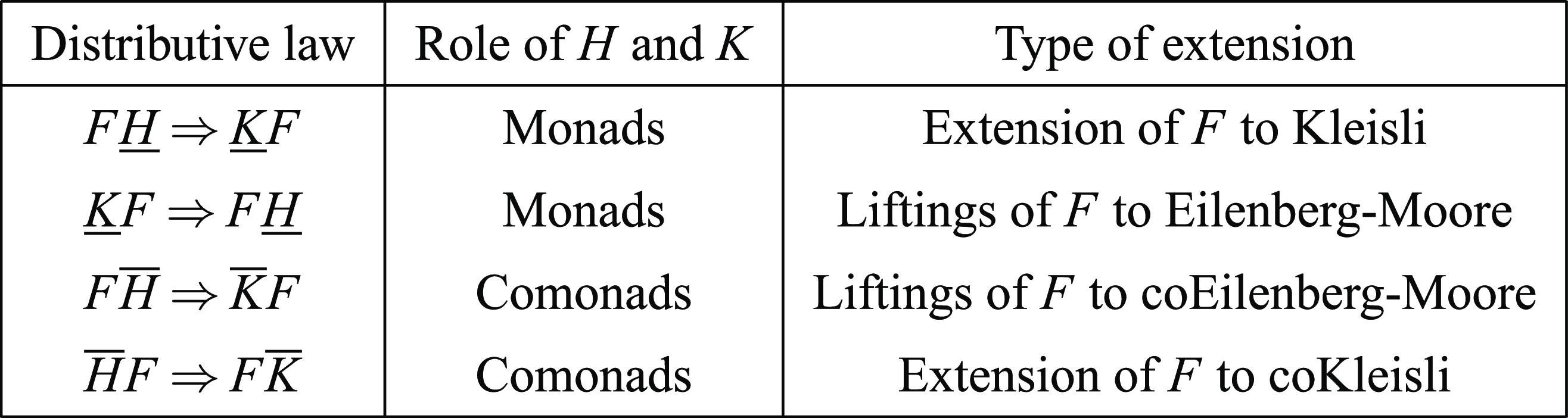
We summarize the different configurations for a distributive law, depending on the direction of the natural transformation and the choice between monads and comonads in Figure 2.
Configurations for distributive laws.

2.4 Distributive laws between monads and comonads
The central notion of this article, Taylor expansion, is given by a distributive law
 $\partial : ! \mathsf {S} \Rightarrow \mathsf {S} !$
between a functor
 $\mathsf {S}$
that represents partial summability (see section 4) and the resource comonad
 $!\_$
of LL (see Definition 98). It turns out that
 $\mathsf {S}$
is a monad, and that
 $\partial : ! \mathsf {S} \Rightarrow \mathsf {S} !$
is also a distributive law between the functor
 $!\_$
, and the monad
 $\mathsf {S}$
. As such, the following notion of distributive law of a comonad over a monad is central to this article.
Definition 16.
Let
 $\underline {M} = (M, \eta, \mu )$
be a monad on a category
 $\mathscr {C}$
, and
 $\overline {D} = (D, \epsilon, \delta )$
be a comonad on
 $\mathscr {C}$
. A distributive law of the comonad
 $\overline {D}$
over the monad
 $\underline {M}$
is a natural transformation
 $\lambda : \overline {D} \underline {M} \Rightarrow \underline {M} \overline {D}$
that is both a distributive law
 $\lambda : D \underline {M} \Rightarrow \underline {M} D$
(
Definition 5
) and a distributive law
 $\lambda : \overline {D} M \Rightarrow M \overline {D}$
(
Definition 12
).
Similarly, there are distributive laws between two monads, as well as distributive laws between two comonads, with similar definitions as above. In fact, distributive laws were first introduced in Beck (Reference Beck and Eckmann1969) between two monads. The notion of distributive law of a comonad over another comonad is also of interest in the article, because the functor
 $\mathsf {S}$
admits a comonadic structure and
 $\partial : ! \mathsf {S} \Rightarrow \mathsf {S} !$
is a distributive law of the comonad
 $!\_$
over the comonad
 $\mathsf {S}$
.
Observe that the following assertions are equivalent, by definition.
-
(1)
 $\lambda$
is a distributive law of the comonad
$\overline {D}$
over the monad
$\underline {M}$
,
-
(2)
$\lambda$
is a distributive law
$D \underline {M} \Rightarrow \underline {M} D$
and
$\epsilon$
and
$\delta$
are morphisms of distributive laws, -
(3)
$\lambda$
is a distributive law
$\overline {D} M \Rightarrow M \overline {D}$
and
$\eta$
and
$\mu$
are morphisms of distributive laws,


where the distributive laws
 $D^2 \underline {M} \Rightarrow \underline {M} D^2$
,
 $\overline {D} M^2 \Rightarrow M^2 \overline {D}$
,
 $\underline {M} \Rightarrow \underline {M}$
and
 $\overline {D} \Rightarrow \overline {D}$
involved above are given by compositionality of the distributive laws, see Remark 9.
By Theorem 14, a distributive law of a comonad over a monad provides a monad
 $\widehat {\underline {M}}$
on
 $\mathscr {C}_{\overline {D}}$
that extends
 $\underline {M}$
. By Theorems 8 and 10, such distributive law also provides a comonad
 $\widehat {\overline {D}}$
on
 $\mathscr {C}_{\underline {M}}$
that extends
 $\overline {D}$
. We can also check that
 $(\mathscr {C}_{\overline {D}})_{\widehat {\underline {M}}} = (\mathscr {C}_{\underline {M}})_{\widehat {\overline {D}}}$
, so a distributive law of a comonad over a monad allows to combine them in arbitrary ways. This result was first proved in Van Osdol (Reference Van Osdol1971).
There is also another notion of distributive laws of the monad
 $\underline {M}$
over the comonad
 $\overline {D}$
obtained by reversing the arrows. Such distributive laws are associated to lifting of the monad
 $\underline {M}$
to the coEilenberg-Moore category of
 $\overline {D}$
, and lifting of
 $\overline {D}$
to the Eilenberg-Moore category of
 $\underline {M}$
.
Those notions of distributive laws between monads and comonads allow in particular to define the notion of bimonad as a functor equipped with a structure of monad and a structure of comonad together with a distributive law expressing that these two structures commute in some sense. Bimonads are formally similar to the notion of Hopf bialgebra in a symmetric monoidal category, apart that the role of the symmetry is played here by the distributive law.
Definition 17 (6.2 of Mesablishvili and Wisbauer (Reference Mesablishvili and Wisbauer2011)). Assume that
 $\overline {H} = (H, \eta, \mu )$
is a monad on
 $\mathscr {C}$
and
 $\underline {H} = (H, \epsilon, \delta )$
is a comonad on
 $\mathscr {C}$
. Then
 $(H, \eta, \mu, \epsilon, \delta )$
is a
 $\tau$
-bimonad if
 $\tau$
is a distributive law
 $\overline {H} \underline {H} \Rightarrow \underline {H} \overline {H}$
of the monad
 $\overline {H}$
over the comonad
 $\underline {H}$
, and a distributive law
 $\underline {H} \overline {H} \Rightarrow \overline {H} \underline {H}$
of the comonad
 $\underline {H}$
over the monad
 $\overline {H}$
, and if the diagrams below commute.

Recall that
 $\ast$
is defined as the horizontal composition of natural transformations: if
 $F, G : \mathscr {C} \rightarrow \mathscr {D}$
,
 $F', G' : \mathscr {D} \rightarrow \mathscr {E}$
,
 $\alpha : F \Rightarrow G$
and
 $\beta : F' \Rightarrow G'$
, then
 $\beta \ast \alpha : GF \Rightarrow G' F'$
is defined as
 \begin{equation} (\beta \ast \alpha )_X = \beta _{F' X} \circ G \alpha _X = G' \alpha _X \circ \beta _{F X}. \end{equation}
Remark 18.
There is a difference between
 $\tau$
-bimonads and bimonads as introduced in 4.1 of Mesablishvili and Wisbauer (Reference Mesablishvili and Wisbauer2011). Every
 $\tau$
-bimonad is a bimonad, but the converse is not true. Still,
 $\tau$
is a part of the
 $\tau$
-bimonad structure and as such should not be explicitly referenced by the terminology. Furthermore, all the bimonads under consideration in our article are
 $\tau$
-bimonads. Thus, we will refer to
 $\tau$
-bimonads simply as bimonads.
Remark 19.
The four diagram making
 $\tau$
a distributive law
 $\overline {H} \underline {H} \Rightarrow \underline {H} \overline {H}$
are exactly the same as the diagrams making
 $\tau$
a distributive law
 $\underline {H} \overline {H} \Rightarrow \overline {H} \underline {H}$
, except that the arrows involving
 $\tau$
are reversed. In particular, if
 $\tau$
is involutive then any of the two assumptions implies the other.
3. Background: Symmetric Monoidal Monads as Distributive Laws
An important concept in the theory of monads (and in this article) is the concept of lax symmetric monoidal functor and lax symmetric monoidal monad. This concept is important because if
 $\mathscr {L}$
is a symmetric monoidal category and
 $\underline {M}$
is a monad on
 $\mathscr {L}$
, then
 $\mathscr {L}_{\underline {M}}$
inherits from
 $\mathscr {L}$
the structure of a symmetric monoidal category as first shown in Day (Reference Day, MacLane, Applegate, Barr, Day, Dubuc, Phreilambud, Street, Tierney and Swierczkowski1970). As expected, this notion is then deeply connected to the notion of distributive laws, and we discuss this connection in this section.
Lax monoidal structures can also be expressed in terms of strength, see Kock (Kock (Reference Kock1970, Reference Kock1972). We detail this process as the notion of strength crucially allows us to define a theory of Taylor expansion with regard to only one parameter in Section 7.2.
3.1 Distributive laws on product categories
Let us recall first some fact and notation about product categories. The category
 $\mathbf {Cat}$
whose objects are the (small) categories and whose morphisms are the functors is a cartesian category, with terminal object the category
 $\mathbf {1}$
which contains one object and one morphism, and whose categorical product is defined as follows.
Given two categories
 $\mathscr {C}_1$
and
 $\mathscr {C}_2$
, the product category
 $\mathscr {C}_1 \times \mathscr {C}_2$
is the category whose objects are the pairs
 $(X_1, X_2)$
with
 $X_1 \in \mathbf {Obj}(\mathscr {C}_1)$
and
 $X_2 \in \mathbf {Obj}(\mathscr {C}_2)$
and whose morphisms are the pairs
 $(f_1, f_2)$
with
 $f_1 \in \mathscr {C}_1(X_1, Y_1)$
and
 $f_2 \in \mathscr {C}_2(X_2, Y_2)$
.
For any functors
 $F_1 : \mathscr {C}_1 \rightarrow \mathscr {D}_1$
and
 $F_2 : \mathscr {C}_2 \rightarrow \mathscr {D}_2$
, we can define the functor
 $F_1 \times F_2 : \mathscr {C}_1 \times \mathscr {C}_2 \rightarrow \mathscr {D}_1 \times \mathscr {D}_2$
by
 $(F_1 \times F_2) (X_1, X_2) = (F_1 X_1, F_2 X_2)$
and
 $(F \times F_2) (f_1, f_2) = (F_1 f_1, F_2 f_2)$
.
Given
 $F_1 : \mathscr {C} \rightarrow \mathscr {D}_1$
and
 $F_2 : \mathscr {C} \rightarrow \mathscr {D}_2$
, we can define
 $\langle F_1, F_2 \rangle : \mathscr {C} \rightarrow \mathscr {D}_1 \times \mathscr {D}_2$
by
 $\langle F_1, F_2 \rangle X = (F_1 X, F_2 X)$
and
 $\langle F_1, F_2 \rangle f = (F_1 f, F_2 f)$
. For any category
 $\mathscr {C}$
, we can define the functor
 $\Delta ^{\mathscr {C}} : \mathscr {C} \rightarrow \mathscr {C} \times \mathscr {C}$
by
 $\Delta ^{\mathscr {C}}(X) = (X, X)$
and
 $\Delta ^{\mathscr {C}} f = (f, f)$
. That is,
 $\Delta ^{\mathscr {C}} = \langle \mathsf {Id}, \mathsf {Id} \rangle$
.
Given the functors
 $F_1, G_1 : \mathscr {C}_1 \rightarrow \mathscr {D}_1$
and
 $F_2, G_2 : \mathscr {C}_2 \rightarrow \mathscr {D}_2$
and two natural transformation
 $\alpha _1 : F_1 \Rightarrow G_1$
and
 $\alpha _2 : F_2 \Rightarrow G_2$
, we can define the natural transformation
 $(\alpha _1, \alpha _2) : F_1 \times F_2 \Rightarrow G_1 \times G_2$
by
 $(\alpha _1, \alpha _2)_{(X_1, X_2)} = (\alpha _{1, X_1}, \alpha _{2, X_2})$
.
Definition 20.
Given a monad
 $\underline {M}_1 = (M_1, \eta _1, \mu _1)$
on
 $\mathscr {C}_1$
and a monad
 $\underline {M}_2 = (M_2, \eta _2, \mu _2)$
on
 $\mathscr {C}_2$
, we can define the monad
 $\underline {M}_1 \times \underline {M}_2$
on
 $\mathscr {C}_1 \times \mathscr {C}_2$
whose unit is
 $(\eta _1, \eta _2)$
and whose sum is
 $(\mu _1, \mu _2)$
.
We can check that
 $(\mathscr {C}_1 \times \mathscr {C}_2)_{\underline {M}_1 \times \underline {M}_2} = \mathscr {C}_{\underline {M}_1} \times \mathscr {C}_{\underline {M}_2}$
, so the following lemmas make sense.
Lemma 21.
The functor
 $\Delta ^{\mathscr {C}_{\underline {M}}} : \mathscr {C}_{\underline {M}} \rightarrow \mathscr {C}_{\underline {M}} \times \mathscr {C}_{\underline {M}}$
is an extension of
 $\Delta ^{\mathscr {C}}$
whose associated distributive law is
 $\mathsf {id}_{\langle M, M \rangle } : \langle M, M \rangle \Rightarrow \langle M, M \rangle$
.
Proof. Straightforward computation.
Lemma 22.
Let
 $F : \mathscr {C}_1 \rightarrow \mathscr {D}_1$
and
 $G : \mathscr {C}_2 \rightarrow \mathscr {D}_2$
. Let
 $\widehat {F}$
be an extension of
 $F$
and
 $\widehat {G}$
an extension of
 $G$
whose associated distributive laws are respectively
 $\lambda$
and
 $\lambda '$
. Then
 $\widehat {F} \times \widehat {G}$
is an extension of
 $F \times G$
whose associated distributive law is
 $(\lambda, \lambda ')$
.
Proof. Straightforward computation.
Lemma 23.
Let
 $F : \mathscr {C} \rightarrow \mathscr {D}_1$
and
 $G : \mathscr {C} \rightarrow \mathscr {D}_2$
. Let
 $\widehat {F}$
be an extension of
 $F$
and
 $\widehat {G}$
an extension of
 $G$
whose associated distributive laws are respectively
 $\lambda ^{F}$
and
 $\lambda '$
. Then
 $\langle \widehat {F}, \widehat {G} \rangle$
is an extension of
 $\langle F, G \rangle$
whose associated distributive law is
 $(\lambda, \lambda ')$
.
Proof.
Observe that
 $\langle \widehat {F}, \widehat {G} \rangle = (\widehat {F} \times \widehat {G}) \Delta ^{\mathscr {C}_{\underline {M}}}$
, so the result follows from Lemmas 21 and 22 and the compositionality of the bijection between extensions and distributive laws
Lemma 24.
For any object
 $A$
of
 $\mathscr {C}$
, the constant endofunctor
 $A^{\mathscr {C}_{\underline {M}}} : \mathscr {C}_{\underline {M}} \rightarrow \mathscr {C}_{\underline {M}}$
is an extension of the constant endofunctor
 $A : \mathscr {C} \rightarrow \mathscr {C}$
. Its associated distributive law is
 $\eta \in \mathscr {C}(A, M A)$
Proof.
The fact that
 $A^{\mathscr {C}_{\underline {M}}}$
is an extension of
 $A$
is immediate. Its associated distributive law is
 $A^{\mathscr {C}_{\underline {M}}}(\mathsf {id}_{M X}) = \mathsf {id}_A^{\mathscr {C}_{\underline {M}}} = \eta$
.
3.2 Lax monoidal functor and lax monoidal monads
We recall in this section basic definitions on symmetric monoidal category and monoidal monads, we refer the reader to Melliès (Reference Melliès2009) for more details. Then we show that any symmetric monoidal monad can be interpreted as a distributive law. This explains why a symmetric monoidality structure on a monad allows to extend the symmetric monoidal structure of the category on which the monad is defined to its Kleisli category.
Definition 25.
A monoidal category
 $(\mathscr {L}, \otimes, 1)$
is a category
 $\mathscr {L}$
equipped with a bifunctor
 $\otimes : \mathscr {L} \times \mathscr {L} \rightarrow \mathscr {L}$
called the tensor product, an object
 $1$
called the unit of the tensor, two natural isomorphisms
 $\rho ^{\otimes }_X \in \mathscr {L}(X \otimes 1, X)$
and
 $\lambda ^{\otimes }_X \in \mathscr {L}(1 \otimes X, X)$
called the right and left unitors, and a natural isomorphism
 $\alpha ^{\otimes }_{X, Y, Z} \in \mathscr {L}((X \otimes Y) \otimes Z, X \otimes (Y \otimes Z))$
called the associator. These isomorphisms are subject to commutations that we will not recall here. The category is symmetric monoidal if there is an additional isomorphism
 $\gamma ^{\otimes }_{X,Y} \in \mathscr {L}(X \otimes Y, Y \otimes X)$
compatible with the monoidal structure.
Definition 26.
A lax symmetric monoidal functor from a symmetric monoidal category
 $(\mathscr {L}, \otimes, 1)$
to another symmetric monoidal category
 $(\mathscr {L}', \bullet, I)$
is a tuple
 $(F, m^0, m^2)$
where
 $F : \mathscr {L} \rightarrow \mathscr {L}'$
is a functor,
 $m^0 \in \mathscr {L}'(I, F 1)$
and
 $m^2_{X,Y} \in \mathscr {L}'(F X \bullet F Y, F (X \otimes Y))$
is a natural transformation that are compatible with the monoidal structure


and compatible with the symmetry.

A strong symmetric monoidal functor is a lax symmetric monoidal functor such that
 $m^0$
is an iso, and
 $m^2$
is a natural isomorphism.
Definition 27.
A monoidal natural transformation between two monoidal functors
 $(F, m^0_F, m^2_F)$
and
 $(G, m^0_G, m^2_G)$
is a natural transformation
 $\alpha : F \Rightarrow G$
such that the following diagram commutes.

There is in fact a 2-category in which the objects are the (small) monoidal categories, the morphisms are the lax monoidal functors, and the 2-cells are the monoidal natural transformations. The composition of two lax monoidal functors is given by the composition of the functor and a suitable composition of their associated natural transformations. The compositions of
 $2$
-cells are the same as the compositions in
 $\mathbf {Cat}$
.
Definition 28.
A lax symmetric monoidal monad on a symmetric monoidal category
 $(\mathscr {L}, \otimes, 1)$
is the data of
 $(M, \eta, \mu, m^0, m^2)$
such that
 $(M, m^0, m^2)$
is a lax symmetric monoidal functor from
 $(\mathscr {L}, \otimes, 1)$
to itself,
 $(M, \eta, \mu )$
is a monad on
 $\mathscr {L}$
, and such that
 $\eta$
and
 $\mu$
are monoidal natural transformations. This last assumption corresponds to the fact that
 $m^0 = \eta _{1} \in \mathscr {L}(1, M 1)$
and to the commutation of the following diagrams.


Lax symmetric monoidal monads are a well-studied notion because they are related to the extension of the symmetric monoidal structure to the Kleisli category.
Theorem 29.
(page 30 of Day (Reference Day, MacLane, Applegate, Barr, Day, Dubuc, Phreilambud, Street, Tierney and Swierczkowski1970)) If
 $\underline {M}$
is a symmetric monoidal monad on
 $\mathscr {L}$
, then the structure of symmetric monoidal category of
 $\mathscr {L}$
extends to
 $\mathscr {L}_{\underline {M}}$
.
It turns out that lax monoidal monads are an example of distributive laws. This observation sheds light on Theorem 29 above, and is doubtlessly folklore, but seems to be often overlooked in the literature. We can trace this observation to Guitart (Reference Guitart1980).Footnote 4
The diagrams of Definition 28 correspond to the fact that the natural transformation
 $m^2 : (\_ \otimes \_) (M \times M) \Rightarrow M (\_ \otimes \_)$
is a distributive law between the functor
 $\_ \otimes \_$
and the monads
 $\underline {M} \times \underline {M}$
and
 $\underline {M}$
. By Theorem 8, it means that
 $\_ \otimes \_$
extends to a functor
 $\_ \widehat {\otimes } \_ : \mathscr {L}_{\underline {M}} \times \mathscr {L}_{\underline {M}} \rightarrow \mathscr {L}_{\underline {M}}$
. Then the commutations of Definition 26 corresponds to the fact that
 $\lambda ^{\otimes }$
,
 $\rho ^{\otimes }$
,
 $\alpha ^{\otimes }$
, and
 $\gamma ^{\otimes }$
are morphisms of distributive laws. The distributive laws involved with
 $\alpha ^{\otimes }$
are given by compositionality, and the distributive laws involved with
 $\lambda ^{\otimes }$
and
 $\rho ^{\otimes }$
are given by Proposition 30 below.
Proposition 30.
For any objects
 $X$
and
 $Y$
, the functor
 $X \widehat {\otimes } \_$
is an extension of
 $X \otimes \_$
with associated distributive law
 $m^2 \circ (\eta _X \otimes \mathsf {id}_{M})$
. Similarly, the functor
 $\_ \widehat {\otimes } Y$
is an extension of
 $\_ \otimes Y$
with associated distributive law
 $m^2 \circ (\mathsf {id}_{M} \otimes \eta _Y)$
.
Proof.
Observe that
 $1 \otimes \_ = (\_ \otimes \_ ) \langle 1, \mathsf {Id} \rangle$
and
 $1 \widehat {\otimes } \_ = (\_ \widehat {\otimes } \_ ) \langle 1^{\mathscr {L}_{\underline {M}}}, \mathsf {Id} \rangle$
. We conclude by compositionality of extensions and distributive laws, using the results of Lemma 23 and Lemma 24.
By Theorem 10, this is equivalent to the fact that
 $\lambda ^{\otimes }$
,
 $\rho ^{\otimes }$
,
 $\alpha ^{\otimes }$
, and
 $\gamma ^{\otimes }$
extend to natural transformations on
 $\mathscr {L}_{\underline {M}}$
. This is why the Kleisli category
 $\mathscr {L}_{\underline {M}}$
of a lax monoidal monad inherits from
 $\mathscr {L}$
the structure of a symmetric monoidal category.
Remark 31.
Dually, there is a notion of a symmetric oplax monoidal functor from a monoidal category
 $(\mathscr {L}, \otimes, 1)$
to another monoidal category
 $(\mathscr {L}', \bullet, I)$
. This is a tuple
 $(F, n^0, n^2)$
where
 $F : \mathscr {C}_1 \rightarrow \mathscr {C}_2$
is a functor,
 $n^0 \in \mathscr {C}_2(F 1, I)$
and
 $n^2_{X,Y} \in \mathscr {C}_2(F (X \otimes Y), F X \bullet F Y)$
is a natural transformation, and such that diagrams similar to the ones of
Definition 26
commute. There is also a notion of symmetric oplax monoidal monad (also called Hopf Monad). In the same way that lax symmetric monoidal monads are related to the distributive laws of
Definition 5
, Hopf monads are related to the distributive laws of
Definition 15
, as observed in Wisbauer (Reference Wisbauer2008). It is not surprising then that a monad
 $\underline {M}$
on
 $\mathscr {L}$
is a Hopf monad if and only if the symmetric monoidal structure of
 $\mathscr {L}$
lifts to the Eilenberg-Moore category of
 $\underline {M}$
, see Moerdijk (Reference Moerdijk2002).
Finally, a symmetric (op)lax monoidal comonad is a comonad
 $\overline {D}$
such that the functor
 $D$
is symmetric (op)lax monoidal, and such that
 $\epsilon, \delta$
are monoidal natural transformations. Again, the structure of an (op)lax monoidal comonad can be seen as a distributive law. Following
Figure 2
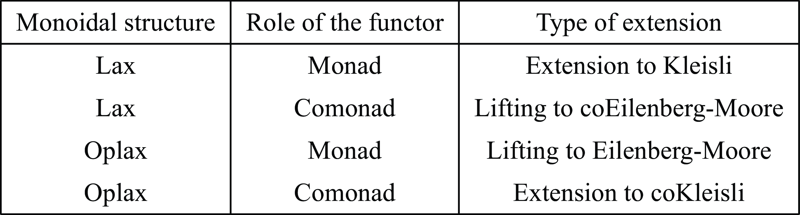
, a lax symmetric monoidal comonad provides a lifting of the symmetric monoidal structure to the coEilenberg-Moore category (see Wisbauer (Reference Wisbauer2008)), and an oplax symmetric monoidal comonad provides an extension of the symmetric monoidal structure to the coKleisli category. We summarize the different results in
Figure 3
.
Extension and lifting of the monoidal structure.

3.3 Commutative monad
It is well known that symmetric monoidal monads are the same as commutative monads, see Kock (Reference Kock1970, Reference Kock1972). Let us recall what is a commutative monad. Let
 $\underline {M}$
be a monad on a symmetric monoidal category
 $\mathscr {L}$
.
Definition 32.
A left strength for
 $\underline {M}$
is a natural transformation
 $\mathsf {t}_{X, Y} \in \mathscr {L}(X \otimes M Y, M (X \otimes Y))$
subject to the compatibility with the monoidal structure

and the compatibility with the monad structure

A right strength is a natural transformation
 $\mathsf {s}_{X, Y} \in \mathscr {L}(M X \otimes Y, M (X \otimes Y))$
subject to similar commutations.
When the category is symmetric monoidal, any left strength
 $\mathsf {t}$
induces a right strength
 \begin{equation} \mathsf {s}_{X,Y} = M \gamma ^{\otimes }_{Y,X} \circ \mathsf {t}_{Y,X} \circ \gamma ^{\otimes }_{X,Y} \end{equation}
and vice versa. This lead to the following naming convention in symmetric monoidal categories.
Definition 33.
A left-strength
 $\mathsf {t}$
for a monad
 $\underline {M}$
is also called a strength.
Definition 34.
A commutative monad is a monad equipped with a strength
 $\mathsf {t}$
such that the following diagram commutes.

where
 $\mathsf {s}$
is the right-strength obtained from
 $\mathsf {t}$
by
Eq. (10)
.
It is well known that any commutative monad is a lax symmetric monoidal monad (see Kock (Reference Kock1970)), defining
 $m^2 \in \mathscr {L}(M X \otimes M Y, M (X \otimes Y))$
as the diagonal of the square above. Conversely, any symmetric monoidal monad is a commutative monad, see Kock (Reference Kock1972). The left and right strengths are defined from the lax monoidal structure by


Recall from Proposition 30 that
 $\mathsf {t}_{X, \_}$
is the distributive law associated to the extension
 $X \widehat {\otimes } \_$
of
 $X \otimes \_$
, and
 $\mathsf {s}_{\_, Y}$
is the distributive law associated to the extension
 $\_ \widehat {\otimes } Y$
of
 $\_ \otimes Y$
. So the equivalence between lax symmetric monoidal monads and commutative monads can also be understood as the fact that providing an extension
 $\_ \widehat {\otimes } \_$
is the same as providing two extensions
 $X \widehat {\otimes } \_$
and
 $\_ \widehat {\otimes } Y$
that follows the compatibility condition of the bifunctor theorem, see proposition 1 of MacLane (Reference MacLane1971).
4. Sigma-Additive Categories and Left Sigma-Summability Structures
Summability structures and left summability structures have been introduced respectively in Ehrhard (Reference Ehrhard2023b) and Ehrhard and Walch (Reference Ehrhard and Walch2023). Both are categorical structures that give to the hom-sets the structure of a finite counterpart of the notions of partially additive monoids (see Arbib and Manes (Reference Arbib and Manes1980)) and
 $\Sigma$
-monoid (see Haghverdi (Reference Haghverdi2000)). The difference between summability structures and left summability structures is that in the former every morphism is linear with regard to the sum (we will call this property additivity), while this is not the case in the latter. Summability structures thus typically appear in models of LL
 $\mathscr {L}$
, while left summability structures appear in the coKleisli categories of their exponential
 $\mathscr {L}_{{!}}$
or in other cartesian closed categories
 $\mathscr {C}$
.
We introduce an infinitary counterpart of those structures, with a key difference in our approach. In Ehrhard (Reference Ehrhard2023b); Ehrhard and Walch (Reference Ehrhard and Walch2023), the
 $\Sigma$
-monoid structure on the hom-set arises naturally from the (left) summability structure itself. Here, we assume that the category is already enriched over
 $\Sigma$
-monoid, and a summability structure is simply a categorical structure that captures this sum. This leads to a simpler theory, that we strongly conjecture to be equivalent to the original one. In all the concrete models we know, the
 $\Sigma$
-monoid structure arises naturally from the categorical structure of the model, such as in the representable case described in section 9.
We work in the framework of left additive structures, because it is more general and is necessary for section 7. Still, we will put a lot of emphasis on the properties of the category of additive morphisms (i.e., morphisms that commutes with the sum), see subsections 4.3 and 4.4, and on summability in the models of LL, see section 5.
Remark 35.
In contrast with bare
 $\Sigma$
-monoid enriched categories, (left) summability structures provide us with an action on objects. This additional structure gives us access to an internal description of summable families which is crucial for representing Taylor expansions (and more generally, the Faà di Bruno formula) within the model.
4.1 Categories enriched over sigma-monoids
If
 $A$
is a countable set and
 $M$
is a set, an
 $A$
-indexed family of elements of
 $M$
is a function
 $\vec {x} : A \rightarrow M$
. We also write
 $\vec {x} = (x_a)_{a \in A}$
. We consider in this section non-empty sets
 $M$
together with a partial function
 $\Sigma$
from indexed family on
 $M$
to
 $M$
called the sum. An indexed family
 $(x_a)_{a \in A}$
is called summable when it is in the domain of
 $\Sigma$
, and we write its image as
 $\sum _{a \in A} x_a$
.
Notation 36.
Borrowing the notations from Tsukada and Asada (Reference Tsukada and Asada2022), for any expressions
 $e$
and
 $e'$
involving sums, we write
-
•
$e \sqsubseteq e'$
if whenever
$e$
is defined, then
$e'$
is defined and
$e = e'$
; -
•
$e \cong e'$
if
$e$
is defined if and only if
$e'$
is defined and
$e = e'$
.


Definition 37. Haghverdi (Reference Haghverdi2000)
The tuple
 $(M, \Sigma )$
is a
 $\Sigma$
-monoid if the sum
 $\Sigma$
satisfies the following axioms.
-
• The unary sum axiom (Unary): any one element family
$x \in M$
is summable of sum
$x$
. -
• The partition associativity axiom (PA): Let
$(x_a)_{a \in A}$
be an indexed family and let
$\{A_i\}_{i \in I}$
be a partition of
$A$
where
$I$
is at most countable and where the
$A_i$
can be potentially empty. Then
(11)
\begin{equation} \sum _{a \in A} x_a \cong \sum _{i \in I} \left (\sum _{a \in A_i} x_a \right ) \! . \end{equation}


It follows from (PA) that any subfamily of a summable family is also summable. In particular, it follows from (PA) and (Unary) that the empty family is always summable (if
 $M$
is not empty). Let
 $0$
be its sum. For any family
 $\vec {x} = (x_a)_{a \in A}$
, we define
 \begin{equation} \mathsf {supp}(\vec {x}) = \{a \in A \mid x_a \neq 0 \}. \end{equation}
Then
 $0$
behaves as the neutral element, as shown in Proposition 38 below.
Proposition 38.
Let
 $\vec {x} = (x_a)_{a \in A}$
be an indexed family, and
 $A'$
a set such that
 $\mathsf {supp}(\vec {x}) \subseteq A' \subseteq A$
. Then
 $(x_a)_{a \in A}$
is summable if and only if
 $(x_a)_{a \in A'}$
is summable and the two sums are equal.
Proof.
Assume that
 $(x_a)_{a \in A'}$
is summable. Then for all
 $a \in A$
, define
 $A_a = \{a\}$
if
 $a \in A'$
, and
 $A_a = \emptyset$
otherwise. Then for all
 $a \in A$
,
 $(x_{a'})_{a' \in A_a}$
is summable of sum
 $x_a$
, by (Unary) and because
 $0$
is the sum over the empty family. It follows from (PA) that
 $(\sum _{a' \in A_a} x_{a'})_{a \in A} = (x_a)_{a \in A}$
is summable of sum
 $\sum _{a \in A'} x_a$
. Conversely, if
 $(x_a)_{a \in A}$
is summable then
 $(x_{a'})_{a \in A'}$
is summable because it is a subfamily, and it is proved above that the sums are equal.
Remark 39. As discussed in Manes and Arbib (Reference Manes and Arbib1986); Hines (Reference Hines2013), the “only if” assumption of the axiom (PA) is very strong, as it implies that the morphisms are positive, in the sense that if
 $x + y = 0$
then
 $x = y = 0$
. Because of this, our axiomatization of summability leaves behind interesting models of LL in which the coefficients are not necessarily nonnegative, but in which maps are definitely analytics, such as Köthe spaces, see Ehrhard (Reference Ehrhard2002), or finiteness spaces, see Ehrhard (Reference Ehrhard2005).
For now, we keep this stronger and fundamentally positive Footnote 5axiomatization because it suits quite well with the situations which occur in the denotational semantics of programming languages and of proofs. A more general axiomatization of summability structure based on the partial commutative monoids of Hines (Reference Hines2013) where the “only if” assumption is dropped is currently a work in progress. It should allow one to recover the partial summability of both finiteness spaces and Köthe spaces.
Definition 40.
If
 $A$
and
 $B$
are indexing sets,
 $\varphi :A \rightarrow B$
is a bijection
 $\vec {x}= (x_a)_{a \in A}$
is a family, we define a B-indexed family
 $\varphi _{\ast }\overrightarrow {x}$
by
 $\varphi _{\ast }\overrightarrow {x}=(x_{\varphi ^{-1}(b)})_{b \in B}$
.
Lemma 41.
For any indexed family
 $\vec {x} = (x_a)_{a \in A}$
and any bijection
 $\varphi : A \rightarrow B$
,
 $\vec {x}$
is summable if and only if
 $\varphi _{\ast } \vec {x}$
is summable, and the two sums are equal.
Proof.
Let
 $A_b = \{\varphi ^{-1}(b)\}$
. By (Unary),
 $(x_a)_{a \in A_b}$
is summable of sum
 $x_{\varphi ^{-1}(b)}$
. Then by (PA),
 $(x_a)_{a \in A}$
is summable if and only if
 $(x_{\varphi ^{-1}(b)})_{b \in B}$
is summable and the two sums are equal.
Definition 42.
We generalize
Definition 40
above. Given two indexing set
 $A$
and
 $B$
, an injection
 $\varphi :A \hookrightarrow B$
and a family
 $\vec {x}= (x_a)_{a \in A}$
we define a
 $B$
-indexed family
 $\varphi _{\ast }\overrightarrow {x}= (y_b)_{b \in B}$
by
 \begin{equation*} y_b= \begin{cases} x_a & if \ b\in \varphi (A) \ and \ \varphi (a)=b\\ 0 & otherwise. \end{cases} \end{equation*}
Lemma 43.
The operation
 $\varphi \to \varphi _{\ast }$
is functorial, that is
 $\mathsf {id}_{\ast }\overrightarrow {x}=\overrightarrow {x}$
and
 $\psi _{\ast }\varphi _{\ast }\overrightarrow {x}=(\psi \circ \varphi )_{\ast }\overrightarrow {x}$
.
Lemma 44.
For any injection
 $\varphi : A \hookrightarrow B$
and any
 $A$
-indexed family
 $\vec {x}$
,
 $\vec {x}$
is summable if and only if
 $\varphi _{\ast } \vec {x}$
is summable, and the two sums are equals.
Proof.
Let
 $\vec {y} = \varphi _{\ast } \vec {x} = (y_b)_{b \in B}$
. By definition,
 $\mathsf {supp}(\vec {y}) \subseteq \mathrm {Im}(\varphi ) \subseteq B$
, so by Proposition 38,
 $\vec {y}$
is summable if and only if
 $(y_b)_{b \in \mathrm {Im}(\varphi )}$
is summable, and the two sums are equal. We conclude by Lemma 41, using the fact that
 $\varphi$
is a bijection between
 $A$
and
 $\mathrm {Im}(\varphi )$
.
We introduce the following terminology, as an analogue of the terminology of additive and left additive categories used in differential categories and cartesian differential categories, see Reference Blute, Cockett and SeelyBlute et al., (2006, 2009). The monoid structure on the hom-set is replaced by a
 $\Sigma$
-monoid structure.
Definition 45.
A left
 $\Sigma$
-additive category is a category
 $\mathscr {C}$
such that for any objects
 $X, Y \in \mathbf {Obj}(\mathscr {C})$
, the hom-set
 $\mathscr {C}(X, Y)$
is a
 $\Sigma$
-monoid, and such that the sum is left distributive over composition: for all objects
 $X, Y, Z$
, for all indexed family
 $(g_b \in \mathscr {C}(Y, Z))_{b \in B}$
and
 $f \in \mathscr {C}(X, Y)$
,
 \begin{equation} \left ( \sum _{b \in B} g_b \right ) \circ f \sqsubseteq \sum _{b \in B} g_b \circ f. \end{equation}
A morphism
 $h \in \mathscr {C}(Y, Z)$
is
 $\Sigma$
-additive if for all indexed family
 $(f_a \in \mathscr {C}(X, Y))_{a \in A}$
 \begin{equation} h \circ \left (\sum _{a \in A} f_a \right ) \sqsubseteq \sum _{a \in a} (h \circ f_a). \end{equation}
A
 $\Sigma$
-additive category is a left
 $\Sigma$
-additive category in which all morphisms are
 $\Sigma$
-additive. A
 $\Sigma$
-additive category can also be defined as a category enriched over the category of
 $\Sigma$
-monoids, see Haghverdi (Reference Haghverdi2000).
We want to stress however that (left)
 $\Sigma$
-additive categories are not necessarily (left) additive categories. The sum of a
 $\Sigma$
-monoid may be defined on some infinite indexed families, but undefined on some finite indexed family. None of the examples of
 $\Sigma$
-additive categories given in section 11 are additive categories.
Let
 $0^{X, Y}$
be the zero of the
 $\Sigma$
-monoid structure of
 $\mathscr {C}(X, Y)$
. It follows from the definition that for any
 $f \in \mathscr {C}(X, Y)$
,
 $0^{Y, Z} \circ f = 0^{X, Y}$
, and that for any
 $\Sigma$
-additive
 $h \in \mathscr {C}(Y, Z)$
,
 $h \circ 0^{X, Y} = 0^{X, Z}$
. We will often omit the superscript and simply write
 $0$
.
Distributivity of the left and on the right implies double distributivity, thanks to the axiom (PA).
Proposition 46.
For any left
 $\Sigma$
-additive category
 $\mathscr {C}$
, any indexed family
 $(f_a \in \mathscr {C}(X, Y))_{a \in A}$
and any indexed family
 $(h_b \in \mathscr {C}(Y, Z))_{b \in B}$
such that
 $h_b$
is
 $\Sigma$
-additive for all
 $b \in B$
,
 \begin{equation*} \left (\sum _{b \in B} h_b \right ) \circ \left (\sum _{a \in A} f_a \right ) \sqsubseteq \sum _{(a, b) \in A \times B} (h_b \circ f_a)\,. \end{equation*}
Proof.
By left distributivity and additivity of the
 $h_b$
 \begin{equation*} \left (\sum _{b \in B} h_b \right ) \circ \left (\sum _{a \in A} f_a \right ) \sqsubseteq \sum _{b \in B} \left ( h_b \circ \left ( \sum _{a \in A} f_a \right ) \right ) \sqsubseteq \sum _{b \in B} \sum _{a \in A} (h_b \circ f_a).\end{equation*}
But the sets
 $A \times \{b\}$
are a partition of
 $A \times B$
, so (PA) ensures that
 \begin{equation*} \sum _{(a, b) \in A \times B} (h_b \circ f_a) \cong \sum _{b \in B} \sum _{a \in A} (h_b \circ f_a). \end{equation*}
Corollary 47.
For any summable family
 $(h_b)_{b \in B}$
such that
 $h_b \in \mathscr {C}(Y, Z)$
is
 $\Sigma$
-additive for all
 $b \in B$
,
 $\sum _{b \in B} h_b$
is
 $\Sigma$
-additive.
Proof.
Let
 $(f_a \in \mathscr {C}(X, Y))_{a \in A}$
be a summable family. It follows from Proposition 46 that
 \begin{equation*} \left (\sum _{b \in B} h_b \right ) \circ \left (\sum _{a \in A} f_a \right ) \sqsubseteq \sum _{(a, b) \in A \times B} (h_b \circ f_a) \end{equation*}
Then, the sets
 $\{a\} \times B$
are a partition of
 $A \times B$
, so it follows from (PA) that
 \begin{equation*} \sum _{(a, b) \in A \times B} (h_b \circ f_a) \cong \sum _{a \in A} \sum _{b \in B} (h_b \circ f_a) \end{equation*}
Finally, we know by left distributivity that
 \begin{equation*} \sum _{b \in B} (h_b \circ f_a) = \left ( \sum _{b \in B} h_b \right ) \circ f_a. \end{equation*}
It follows that
 \begin{equation*} \left (\sum _{b \in B} h_b \right ) \circ \left (\sum _{a \in A} f_a \right ) \sqsubseteq \sum _{a \in A} \left ( \left ( \sum _{b \in B} h_b \right ) \circ f_a \right ). \end{equation*}
Remark 48.
In Ehrhard and Walch (Reference Ehrhard and Walch2023), additive morphisms only preserve finite summations (including
 $0$
), which corresponds to the usual algebraic notion of morphism of monoid. In our
 $\Sigma$
-summability setting, additivity means not only preservation of finite sums, but also of all infinite sums when they are defined. This means that
 $\Sigma$
-additive morphisms also feature a property of continuity whose precise nature depends on the category
 $\mathscr {C}$
at stake.
A very interesting situation occurs when the
 $\Sigma$
-monoid structure of
 $\mathscr {C}$
satisfies three additional properties
-
(1) a family
$\overrightarrow {f}\in \mathscr {C}(X,Y)^{\mathbb {N}}$
is summable as soon as, for any finite set
$A$
and any injection
$\varphi :A\to \mathbb {N}$
, the family
$\varphi _{\ast }\overrightarrow {f}$
is summable;
-
(2) the preorder relation
$\leq$
defined on hom-sets of
$\mathscr {C}$
by
$f\leq g$
if
$\exists h\in \mathscr {C}(X,Y)$
such that
$g=f+h$
(where
$+$
is the binary addition induced by
$\Sigma$
) is antisymmetric, that is, is an order relation;
-
(3) if for any finite subset
$A'$
of
$A$
one has
$\sum _{a \in A'} f_a \leq f$
, then
$\sum _{a \in A} f_a \leq f$
.


The first condition turns the structure of
 $\sum$
-monoid into a partially additive monoid, and the two other conditions turn this partially additive monoid into an additive domain, see Section 9.3 of Manes and Arbib (Reference Manes and Arbib1986). When these conditions hold, each hom-set
 $\mathscr {C}(X,Y)$
is easily seen to be an
 $\omega$
-complete partial order (ordered by
 $\leq$
and having
 $0$
as least element). The least upper bound (lub) of
 $(\sum _{i=0}^n f_i)_{n \in \mathbb {N}}$
is given by
 $\sum _{i \in \mathbb {N}} f_i$
. Then,
 $\Sigma$
-additive morphisms are continuous because they commute with the corresponding lubs in the sense that
 $h\circ {\sup _{i\in \mathbb {N}}g_i} = \sup _{i\in \mathbb {N}} (h \circ g_i)$
when
 $h\in \mathscr {C}(Y,Z)$
is
 $\Sigma$
-additive and
 $\overrightarrow {g}\in \mathscr {C}(X,Y)^{\mathbb {N}}$
is a monotone sequence.
All the examples provided in Section 9.8 are instances of this situation and, for that reason, feature general fixpoint operators allowing to combine our coherent Taylor structures with general recursion in the spirit of Ehrhard (Reference Ehrhard2023a).
4.2 Sigma-summability structures
We assume in this section that
 $\mathscr {C}$
is a left
 $\Sigma$
-additive category.
Definition 49.
A left
 $\Sigma$
-summability structure on
 $\mathscr {C}$
is a tuple
 $(\mathsf {S}, (\pi _i)_{i \in \mathbb {N}})$
where
 $\mathsf {S}$
is a map (functional class) on objects
 $\mathsf {S}: \mathbf {Obj}(\mathscr {C}) \rightarrow \mathbf {Obj}(\mathscr {C})$
and each
 $\pi _i$
(for
 $i\in \mathbb {N}$
) is a family of morphisms
 $(\pi _{i,X}\in \mathscr {C}(\mathsf {S} X,X))_{X\in \mathbf {Obj}(\mathscr {C})}$
called the projections such that:
-
SS-1 For any
$X$
,
$(\pi _{i, X})_{i \in \mathbb {N}}$
is jointly monic. Joint monicity means that for any
$f, g \in \mathscr {C}(X, \mathsf {S} Y)$
, if
$\pi _{i, Y} \circ f = \pi _{i,Y} \circ g$
for any
$i \in \mathbb {N}$
, then
$f = g$
. -
SS-2 For any
$\mathbb {N}$
-indexed family,
$(f_i \in \mathscr {C}(X, Y))_{i \in \mathbb {N}}$
is summable if and only if there exists a morphism
$f \in \mathscr {C}(X, \mathsf {S} Y)$
such that
$\forall i\in \mathbb {N}, \pi _i \circ f = f_i$
. -
SS-3 For any object
$X$
, the morphisms
$(\pi _{i, X})_{i \in \mathbb {N}}$
are
$\Sigma$
-additive.
-
SS-4 For any
$A$
-indexed family
$(f_a \in \mathscr {C}(X, \mathsf {S} Y))_{a \in A}$
, if
$(\pi _{i, Y} \circ f_a)_{(i, a) \in \mathbb {N} \times A}$
is summable then
$(f_a)_{a \in A}$
is summable.


The subscript
 $X$
is usually omitted when writing projections
 $\pi _{i,X}$
.
Definition 50.
A left
 $\Sigma$
-summability structure on a
 $\Sigma$
-additive category is called a
 $\Sigma$
-summability structure.
Notation 51.
Because of SS-1
, the morphism
 $f$
given in SS-2
is unique and is called witness of
 $(f_i)_{i \in \mathbb {N}}$
. We write
 $\left \langle \!\left \langle f_i \right \rangle \!\right \rangle _{i \in \mathbb {N}} = f$
.
Intuitively, SS-1 and SS-2 mean that
 $\mathsf {S} X$
can be seen as the object of ”summable sequences”. The morphism
 $\pi _i$
maps a sequence to its
 $i$
-th element. Then, SS-3 ensures that the sums between sequences is given by the sum on each component
 \begin{equation*} \pi _i \circ \sum _{a \in A} \left \langle \!\left \langle f_{i,a} \right \rangle \!\right \rangle _{i \in \mathbb {N}} \sqsubseteq \sum _{a \in A} f_{i,a} \text { so } \sum _{a \in A} \left \langle \!\left \langle f_{i,a} \right \rangle \!\right \rangle _{i \in \mathbb {N}} = \left \langle \!\left \langle \sum _{a \in A} f_{i, a} \right \rangle \!\right \rangle _{i \in \mathbb {N}}. \end{equation*}
Finally, SS-4 crucially ensures that
 $(\left \langle \!\left \langle f_{i,a} \right \rangle \!\right \rangle _{i \in \mathbb {N}})_{a \in A}$
is summable if and only if
 $(f_{i,a})_{(i,a) \in \mathbb {N} \times A}$
is summable (the only if is a consequence of double distributivity, see Proposition 46). So the summability of sequences is completely determined by the global summability of all of their components.
Example 52.
The models of Taylor expansion introduced in Manzonetto (Reference Manzonetto2012) are assumed to feature arbitrary countable sums. Then these sums correspond to a particular (left)
 $\Sigma$
-summability structure defined as
 $\mathsf {S} X = \&_{i \in \mathbb {N}} X$
,
 $\pi _i = \mathsf {p}_i$
(where
 $\&$
is a countable categorical product and
 $\mathsf {p}_i$
is the
 $i$
projection). This setting is covered in depth in Section 10.2
. Note that in general,
 $\mathsf {S} X$
is not the cartesian product, precisely because the sum is partial so the witness of a family of morphism needs not always exist.
Notation 53.
By SS-2
, the projections
 $(\pi _i)_{i \in \mathbb {N}}$
are summable with witness
 $\mathsf {id}$
. Let
 $\sigma _X = \sum _{i \in \mathbb {N}} \pi _{i,X} \in \mathscr {C}(\mathsf {S} X, X)$
.
We now assume that
 $\mathscr {C}$
is equipped with a left
 $\Sigma$
-summability structure. Observe that by left distributivity,
 \begin{equation} \sigma \circ \left \langle \!\left \langle f_i \right \rangle \!\right \rangle _{i \in \mathbb {N}} \sqsubseteq \sum _{i \in \mathbb {N}} (\pi _i \circ \left \langle \!\left \langle f_i \right \rangle \!\right \rangle _{i \in \mathbb {N}}) = \sum _{i \in \mathbb {N}} f_i. \end{equation}
Thus, the data of
 $(\mathsf {S}, (\pi _i)_{i \in \mathbb {N}}, \sigma )$
completely characterize the summability and the values of sums on
 $\mathbb {N}$
-indexed families. By Lemma 44, this is enough to characterize the
 $\Sigma$
-monoid structure on all indexed family, because any countable set has an injection into
 $\mathbb {N}$
. This explains why earlier versions of this paper define summability structures first, and the
 $\Sigma$
-monoid structure simply arise as a by-product. The definition of sum of those earlier version were similar to the characterization given by Proposition 54 below.
Proposition 54.
A family
 $\vec {f} = (f_a \in \mathscr {C}(X, Y))_{a \in A}$
is summable if and only if there exists an injection
 $\varphi : A \hookrightarrow \mathbb {N}$
and a morphism
 $\langle \!\langle \vec {f} \rangle \!\rangle ^{\varphi } \in \mathscr {C}(X, \mathsf {S} Y)$
such that
 $\langle \!\langle \vec {f} \rangle \!\rangle ^{\varphi }$
is a witness for
 $\varphi _{\ast } f$
. That is,
 \begin{equation*} \pi _i \circ \langle \!\langle \vec {f} \rangle \!\rangle ^{\varphi } = \begin{cases} f_a\ if \ i = \varphi (a) \ for\ some\ a \in A \\ 0 \ otherwise. \end{cases} \end{equation*}
Furthermore,
 $\sum _{a \in A} f_a = \sigma \circ \langle \!\langle \vec {f} \rangle \!\rangle ^{\varphi }$
.
Proof. This is a direct consequence of SS-2 and Lemma 44 and Eq. (15).
The characterization of summability in terms of the existence of witnesses implies that properties involving summability can often be expressed in terms of the basic data of the summability structure. This is the case for instance of the additivity of morphisms.
Proposition 55.
For any morphism
 $h$
, the following assertions are equivalent.
-
(1)
$h$
is
$\Sigma$
-additive;
-
(2)
$h \circ 0 = 0$
and
$(h \circ \pi _i)_{i \in \mathbb {N}}$
is summable with sum
$h \circ \sigma$
.


Proof.
The forward implication is a direct consequence of the definition of additivity applied on the empty family and on the summable family
 $(\pi _i)_{i \in \mathbb {N}}$
. For the backward implication, assume that
 $\vec {f} = (f_a)_{a \in A}$
is summable. By Proposition 54, there exists an injection
 $\varphi : A \hookrightarrow \mathbb {N}$
and a witness
 $\langle \!\langle \vec {f} \rangle \!\rangle ^{\varphi }$
of
 $\varphi _{\ast } \vec {f}$
. Then we can check that
 $\left \langle \!\left \langle h \circ \pi _i \right \rangle \!\right \rangle _{i \in \mathbb {N}} \circ \langle \!\langle \vec {f} \rangle \!\rangle ^{\varphi }$
is a witness for
 $\varphi _{\ast } (h \circ f_a)_{a \in A}$
. Indeed,
 \begin{equation*} h \circ \pi _i \circ \langle \!\langle \vec {f} \rangle \!\rangle ^{\varphi } = \begin{cases} h \circ f_a \text { if } i \in \varphi (A) \text { and } \varphi (a) = i \\ h \circ 0 = 0 \text { otherwise.} \end{cases} \end{equation*}
Thus, by Proposition 54,
 $(h \circ f_a)_{a \in A}$
is summable with sum
 \begin{equation*} \sum _{a \in A} h \circ f_a = \sigma \circ \left \langle \!\left \langle h \circ \pi _i \right \rangle \!\right \rangle _{i \in \mathbb {N}} \circ \langle \!\langle \vec {f} \rangle \!\rangle ^{\varphi } = h \circ \sigma \circ \langle \!\langle \vec {f} \rangle \!\rangle ^{\varphi } = h \circ \sum _{a \in A} f_a.\end{equation*}
It concludes the proof.
Notation 56.
As for any family, we use the notation
 $\vec {\pi }$
for the family of projections
 $(\pi _i)_{i \in \mathbb {N}}$
.
4.3 The category of sigma-additive morphisms
We assume in this section that
 $\mathscr {C}$
is a left
 $\Sigma$
-additive category. It is easy to show that the identity morphism
 $\mathsf {id}_X \in \mathscr {C}(X, X)$
is
 $\Sigma$
-additive, and that the composition of two
 $\Sigma$
-additive morphisms is also
 $\Sigma$
-additive.
Definition 57.
Let
 $\mathscr {C}^{\mathsf {add}}$
be the category whose objects are those of
 $\mathscr {C}$
and whose morphisms are the
 $\Sigma$
-additive morphisms of
 $\mathscr {C}$
We use
 $h'\, h$
for
 $h'\circ h$
when
 $h$
and
 $h'$
are
 $\Sigma$
-additive to stress the fact that additivity is a form of linearity.
There is an obvious forgetful functor from
 $\mathscr {C}^{\mathsf {add}}$
to
 $\mathscr {C}$
that we always keep implicit. It follows from Corollary 47 that
 $\mathscr {C}^{\mathsf {add}}$
is a
 $\Sigma$
-additive category. We now assume that
 $\mathscr {C}$
is equipped with a left
 $\Sigma$
-summability structure
 $(\mathsf {S}, \vec {\pi })$
.
Lemma 58.
For all summable family
 $(h_i \in \mathscr {C}(Y,Z))_{a \in A}$
of
 $\Sigma$
-additive morphisms,
 $\left \langle \!\left \langle h_i \right \rangle \!\right \rangle _{i \in \mathbb {N}}$
is
 $\Sigma$
-additive.
Proof.
Assume that
 $(f_a \in \mathscr {C}(X, Y))_{a \in A}$
is summable. We first want to show that
 $(\left \langle \!\left \langle h_i \right \rangle \!\right \rangle _{i \in \mathbb {N}} \circ f_a)_{a \in A}$
is summable. By SS-4, it suffices to show that
 $(h_i \circ f_a)_{(i, a) \in \mathbb {N} \times A}$
is summable. This is the case, by double distributivity (Proposition 46). Then, we show that
 \begin{equation*} \left \langle \!\left \langle h_i \right \rangle \!\right \rangle _{i \in \mathbb {N}} \circ \left (\sum _{a \in A} f_a \right ) = \sum _{a \in A} (\left \langle \!\left \langle h_i \right \rangle \!\right \rangle _{i \in \mathbb {N}} \circ f_a).\end{equation*}
This is done in a straightforward way using the additivity and the joint monicity of the
 $\pi _i$
.
Proposition 59.
 $(\mathsf {S}, \vec {\pi })$
is also a
 $\Sigma$
-summability structure on
 $\mathscr {C}^{\mathsf {add}}$
.
Proof.
Both SS-1 and SS-3 hold by assumption. The property SS-4 follows from the fact that the summability in
 $\mathscr {C}^{\mathsf {add}}$
coincides with the summability in
 $\mathscr {C}$
. Finally, SS-2 follows from Lemma 58 above.
Recall Proposition 55: a morphism
 $h$
is
 $\Sigma$
-additive if and only if
 $(h \circ \pi _i)_{i \in \mathbb {N}}$
is summable with sum
 $h \circ \sigma$
. We define
 \begin{equation} \mathsf {S} h = \left \langle \!\left \langle h \circ \pi _i \right \rangle \!\right \rangle _{i \in \mathbb {N}} \end{equation}
so that
 $\pi _i \circ \mathsf {S} h = h \circ \pi _i$
. Furthermore,
 $\sigma \circ \mathsf {S} h = h \circ \sigma$
by Eq. (15). We can easily check by joint monicity of the
 $\pi _i$
that
 $\mathsf {S} h \circ \left \langle \!\left \langle x_i \right \rangle \!\right \rangle _{i \in \mathbb {N}} = \left \langle \!\left \langle h \circ x_i \right \rangle \!\right \rangle _{i \in \mathbb {N}}$
, so
 $\mathsf {S} h$
consists intuitively in applying
 $h$
in each argument.
Proposition 60.
 $\mathsf {S}$
is an endofunctor on
 $\mathscr {C}^{\mathsf {add}}$
, and the
 $\pi _i$
and
 $\sigma$
are natural transformations.
Proof.
Observe first that for all
 $h \in \mathscr {C}^{\mathsf {add}}(X, Y)$
,
 $\mathsf {S} h \in \mathscr {C}^{\mathsf {add}}(\mathsf {S} X, \mathsf {S} Y)$
by definition of
 $\mathsf {S} h$
and Lemma 58. Then
 \begin{equation*} \pi _i \circ \mathsf {S} \mathsf {id}_X = \mathsf {id}_{X} \circ \pi _i = \pi _i = \pi _i \circ \mathsf {id}_{\mathsf {S} X} \end{equation*}
so
 $\mathsf {S} \mathsf {id}_X = \mathsf {id}_{\mathsf {S} X}$
by joint monicity of the
 $\pi _i$
. Then, assume that
 $h \in \mathscr {C}(X, Y)$
and
 $h' \in \mathscr {C}(Y, Z)$
are
 $\Sigma$
-additive.
 \begin{equation*} \pi _i \circ \mathsf {S} h' \circ \mathsf {S} h = h' \circ \pi _i \circ \mathsf {S} h = h' \circ h \circ \pi _i = \pi _i \circ \mathsf {S} (h' \circ h) \end{equation*}
so
 $\mathsf {S} (h' \circ h) = \mathsf {S} h' \circ \mathsf {S} h$
by joint monicity of the
 $\pi _i$
. Thus,
 $\mathsf {S}$
is a functor, and we already know that
 $\pi _i \, \mathsf {S} h = h \, \pi _i$
,
 $\sigma \, \mathsf {S} h = h \, \sigma$
, so they are natural transformations.
Proposition 61.
For all family
 $(h_a)_{a \in A}$
of
 $\Sigma$
-additive morphisms,
 \begin{equation*} \mathsf {S} \left ( \sum _{a \in A} h_a \right ) \cong \sum _{a \in A} (\mathsf {S} h_a) \end{equation*}
Proof.
Let
 $\varphi : A \hookrightarrow \mathbb {N}$
be an injection. Assume that
 $(h_a)_{a \in A}$
is summable. Then
 $(h_i')_{i \in \mathbb {N}} = \varphi _{\ast }{(h_a)_{a \in A}}$
is summable by Lemma 44. So by double distributivity,
 \begin{equation*} (h_i' \, \pi _j)_{(i, j) \in \mathbb {N} \times \mathbb {N}} = (\pi _j \, \mathsf {S} h_i')_{(i, j) \in \mathbb {N} \times \mathbb {N}} \end{equation*}
is summable. It follows by SS-4 that
 $(\mathsf {S} h_i')_{i \in \mathbb {N}}$
is summable. But
 $\mathsf {S} 0 = 0$
(this directly follows from the joint monicity of the
 $\pi _i$
). So
 $(\mathsf {S} h_i')_{i \in \mathbb {N}} = \varphi _{\ast }{(\mathsf {S} h_a)_{a \in A}}$
and
 $(\mathsf {S} h_a)_{a \in A}$
is summable by Lemma 44. Furthermore,
 \begin{equation*} \pi _i \, \mathsf {S} \left ( \sum _{a \in A} h_a \right ) = \left ( \sum _{a \in A} h_a \right ) \, \pi _i \sqsubseteq \sum _{a \in A} (h_a \, \pi _i) \end{equation*}
 \begin{equation*} \pi _i \, \left ( \sum _{a \in A} \mathsf {S} h_a \right ) \sqsubseteq \sum _{a \in A} (\pi _i \, \mathsf {S} h_a) = \sum _{a \in A} (h_a \, \pi _i) \end{equation*}
so by joint monicity of the
 $\pi _i$
, the two sums are equal.
To conclude the proof, assume that
 $(\mathsf {S} h_a)_{a \in A}$
is summable and let us show that
 $(h_a)_{a \in A}$
is summable. As observed above,
 $(\mathsf {S} h_i')_{i \in \mathbb {N}} = \varphi _{\ast }{(\mathsf {S} h_a)_{a \in A}}$
so this family is summable by Lemma 44. It follows by double distributivity that
 $(\pi _j \, \mathsf {S} h_i')_{(i, j) \in \mathbb {N} \times \mathbb {N}} = (h_i' \, \pi _j)_{(i, j) \in \mathbb {N} \times \mathbb {N}}$
is summable.
Then, let
 $\iota _i \in \mathscr {C}(X, \mathsf {S} X)$
be the morphism such that
 $\pi _i \circ \iota _i = \mathsf {id}_X$
and
 $\pi _j \circ \iota _i = 0$
if
 $j \neq i$
. This morphism exists thanks to (Unary) and SS-2. Then by left distributivity in
 $\mathscr {C}$
,
 $(h_i' \circ \pi _j \circ \iota _0)_{(i, j) \in \mathbb {N} \times \mathbb {N}}$
is summable. This indexed family has values
 $h_i'$
on indexes
 $(i, 0)$
, and values
 $0$
on any index
 $(i, j)$
such that
 $j \neq 0$
, by additivity of
 $h_i'$
. So by Proposition 38 and Lemma 41,
 $(h_i')_{i \in \mathbb {N}}$
is summable and thus
 $(h_a)_{a \in A}$
is summable by Lemma 44.
Finally, we show that naturality in
 $\mathscr {C}^{\mathsf {add}}$
is preserved by witness and sums.
Lemma 62.
For any category
 $\mathscr {D}$
and all functors
 $F, G : \mathscr {D} \rightarrow \mathscr {C}^{\mathsf {add}}$
,
 $0$
is a natural transformation
 $F \Rightarrow G$
.
Proof.
We have
 $0 \, F f = 0 = G f \, 0$
by additivity of
 $G f$
.
Definition 63.
Let
 $\mathscr {D}$
be a category, and
 $F, G : \mathbf {Obj}(\mathscr {D}) \rightarrow \mathbf {Obj}(\mathscr {C})$
two maps. Assume that for all
 $a \in A$
,
 $\alpha ^a = (\alpha ^a_X)_{X \in \mathbf {Obj}(\mathscr {D})}$
is a family of morphisms with
 $\alpha ^a_X \in \mathscr {C}(F X, G X)$
. We say that
 $(\alpha ^a)_{a \in A}$
is summable if for all object
 $X$
,
 $(\alpha ^a_X)_{a \in A}$
is summable. Then we write
 $\sum _{a \in I} \alpha ^a$
the family
 $(\sum _{a \in A} \alpha ^a_X)_X$
. If
 $A = \mathbb {N}$
, we write
 $\left \langle \!\left \langle \alpha ^i \right \rangle \!\right \rangle _{i \in \mathbb {N}}$
the family
 $(\left \langle \!\left \langle \alpha ^i_X \right \rangle \!\right \rangle _{i \in \mathbb {N}})_X$
.
Proposition 64.
The sums and witnesses of natural transformations in
 $\mathscr {C}^{\mathsf {add}}$
are also natural transformations. More precisely, for any category
 $\mathscr {D}$
, for all functors
 $F, G : \mathscr {D} \rightarrow \mathscr {C}^{\mathsf {add}}$
and for any family
 $(\alpha ^a)_{a \in A}$
of natural transformations
 $\alpha ^a : F \Rightarrow G$
, if
 $(\alpha ^a)_{a \in A}$
is summable, then
 $\sum _{a \in A} \alpha ^a$
is a natural transformation
 $F \Rightarrow G$
. If
 $A = \mathbb {N}$
, then
 $\left \langle \!\left \langle \alpha ^i \right \rangle \!\right \rangle _{i \in \mathbb {N}}$
is a natural transformation
 $F \Rightarrow \mathsf {S} G$
.
Proof.
Assume first that
 $A = \mathbb {N}$
. We want to show that
 $\left \langle \!\left \langle \alpha _X^i \right \rangle \!\right \rangle _{i \in \mathbb {N}} \in \mathscr {C}^{\mathsf {add}}(F X, \mathsf {S} G X)$
is a natural transformation
 $F \Rightarrow \mathsf {S} G$
. That is, for all
 $f \in \mathscr {D}(X, Y)$
,
 \begin{equation*} \left \langle \!\left \langle \alpha _Y^i \right \rangle \!\right \rangle _{i \in \mathbb {N}} \, F f = \mathsf {S} G f \, \left \langle \!\left \langle \alpha _X^i \right \rangle \!\right \rangle _{i \in \mathbb {N}}.\end{equation*}
For all
 $i$
,
 \begin{equation*} \pi _i \, \left \langle \!\left \langle \alpha _Y^i \right \rangle \!\right \rangle _{i \in \mathbb {N}} \, F f = \alpha _Y^i \, F f = G f \, \alpha _X^i = G f \, \pi _i \, \left \langle \!\left \langle \alpha _X^i \right \rangle \!\right \rangle _{i \in \mathbb {N}} = \pi _i \, \mathsf {S} G f \, \left \langle \!\left \langle \alpha _X^i \right \rangle \!\right \rangle _{i \in \mathbb {N}}. \end{equation*}
By joint monicity of the
 $\pi _i$
, we conclude that
 $(\left \langle \!\left \langle \alpha _X^i \right \rangle \!\right \rangle _{i \in \mathbb {N}})_X$
is natural. Furthermore,
 $\sum _{i \in \mathbb {N}} \alpha ^i_X = \sigma _{G X} \, \left \langle \!\left \langle \alpha _X^i \right \rangle \!\right \rangle _{i \in \mathbb {N}}$
is natural since
 $\sigma$
is natural. The case where
 $A$
is an arbitrary countable set immediately follows by Lemma 44 and naturality of
 $0$
.
4.4 The bimonad of sigma-summabibility structures
In this section, we endow
 $\mathsf {S}$
with a structure of bimonad in the sense of Definition 17. The corresponding natural transformations are essential in our approach to Taylor expansion and are similar to natural transformations introduced in tangent categories Rosicky (Reference Rosicky1984) and in coherent differentiation Ehrhard and Walch (Reference Ehrhard and Walch2023).
We will see in section 5 that Taylor expansionFootnote 6 consists in a functor
 $\mathsf {T}$
that extends
 $\mathsf {S}$
to
 $\mathscr {C}$
(in particular,
 $\mathsf {T} X = \mathsf {S} X$
), and that the usual properties of differentiation correspond to the naturality with respect to
 $\mathsf {T}$
of the families of morphisms associated with the bimonad structure of
 $\mathsf {S}$
. We provide an intuition on those natural transformations as operations on formal power series.
It is quite enlightening to write a sequence
 $\left \langle \!\left \langle f_i \right \rangle \!\right \rangle _{i \in \mathbb {N}} \in \mathscr {C}(X, \mathsf {S} Y)$
as a formal power series
 $\sum _{i=0}^{\infty } f_i t^i$
(this series is called the generating function). The reason is that as we will see in section 6, the element at position
 $i$
in
 $\left \langle \!\left \langle f_i \right \rangle \!\right \rangle _{i \in \mathbb {N}}$
can be seen as an order
 $i$
degree of differentiation. This is in fact the reason why we write the projections
 $\pi _i$
starting from index
 $0$
and not from index
 $1$
. Then the projection
 $\pi _i$
maps
 $\sum _{i=0}^{\infty } f_i t^i$
to
 $f_i$
, and the sum maps
 $\sum _{i=0}^{\infty } f_i t^i$
to
 $\sum _{i \in \mathbb {N}} f_i$
(it evaluates the formal power series in
 $t = 1$
). We introduce and recall the following families of morphisms on
 $\mathscr {C}$
.
-
(1) A morphism
$\iota _{i,X} \in \mathscr {C}(X, \mathsf {S} X)$
that intuitively maps an element
$x \in X$
to the monomial
$x t^i$
, this morphism was used in the proof of Proposition 61; -
(2) Remember that we have a morphism
$\sigma _X \in \mathscr {C}(\mathsf {S} X, X)$
that intuitively maps a power series
$\sum _{i \in \mathbb {N}} x_i t^i$
to
$\sum _{i \in \mathbb {N}} x_i$
(it evaluates the series in
$t = 1$
); -
(3) A morphism
$\theta _X \in \mathscr {C}(\mathsf {S}^2 X, \mathsf {S} X)$
that intuitively maps a multivariate formal power series
$\sum x_{i,j} t^i u^j$
to the power series
$\sum _{k \in \mathbb {N}} (\sum _{i+j = k} x_{i,j}) v^k$
; -
(4) A lift morphism
$\mathsf {l}_X \in \mathscr {C}(\mathsf {S} X, \mathsf {S}^2 X)$
that intuitively maps the power series
$\sum _{i \in \mathbb {N}} x_i t^i$
to the power series with two indeterminate
$\sum _{i \in \mathbb {N}} x_i u^i v^i$
; -
(5) A flip operator
$\mathsf {c}_X \in \mathscr {C}(\mathsf {S}^2 X, \mathsf {S}^2 X)$
that intuitively maps the power series
$\sum _{i, j \in \mathbb {N}} x_{i,j} t^i u^j$
to
$\sum _{i, j \in \mathbb {N}} x_{i,j} t^j u^i$
.


We show that those morphisms formally exists thanks to the axioms of (left)
 $\Sigma$
-summability structure, that they are
 $\Sigma$
-additive, that they are natural transformations when considered as morphisms in
 $\mathscr {C}^{\mathsf {add}}$
, and that they provide a bimonad structure to
 $\mathsf {S}$
on
 $\mathscr {C}^{\mathsf {add}}$
(we will recall the commutations that are involved on the fly).
Notation 65.
For any
 $i, j \in \mathbb {N}$
and any morphism
 $f \in \mathscr {C}(X, Y)$
, we use
 $\delta _{i,j} f$
for the morphism which is equal to
 $f$
if
 $i = j$
, and to
 $0$
otherwise.
Theorem 66.
-
(1) For all
$i \in \mathbb {N}$
, there is a morphism
$\iota _i \in \mathscr {C}(X,\mathsf {S} X)$
such that
$\pi _j\circ \iota _i=\delta _{i,j}\mathsf {id}$
(and then
$\sigma \circ \iota _i = \mathsf {id}$
).
-
(2) There is a morphism
$\theta \in \mathscr {C}(\mathsf {S}^2X,\mathsf {S} X)$
such that, for all
$i\in \mathbb {N}$
,
$\pi _i\circ \theta =\sum _{j=0}^i\pi _{i-j}\circ \pi _j$
. -
(3) There is a morphism
$\mathsf {l} \in \mathscr {C}(\mathsf {S} X, \mathsf {S}^2 X)$
called lift such that
$\pi _i \circ \pi _j \circ \mathsf {l} = \delta _{i,j} \pi _i$
. That is,
$\mathsf {l} = \left \langle \!\left \langle \iota _i \circ \pi _i \right \rangle \!\right \rangle _{i \in \mathbb {N}}$
. -
(4) There is a morphism
$\mathsf {c}\in \mathscr {C}(\mathsf {S}^2X,\mathsf {S}^2X)$
such that for all
$i,j\in \mathbb {N}$
, one has
$\pi _i\circ \pi _j\circ \mathsf {c}=\pi _j\circ \pi _i$
.


Proof.
The existence of
 $\iota _i$
is a direct consequence of (Unary) and SS-2. The family
 $(\pi _i \, \pi _j)_{(i, j) \in \mathbb {N}^2}$
is summable by double distributivity (Proposition 46). Thus,
 $\theta$
exists by (PA) and SS-2, and
 $\mathsf {c}$
exists by SS-4. Finally, the family
 $(\iota _i \circ \pi _i)_{i \in \mathbb {N}}$
is summable if and only if
 $(\pi _j \circ \iota _i \circ \pi _i)_{(i, j) \in \mathbb {N}^2}$
is summable by SS-4. But
 \begin{equation*}\pi _j \circ \iota _i \circ \pi _i = \begin{cases} \pi _i \text { if } i = j \\ 0 \text { otherwise.} \end{cases} \end{equation*}
Thus,
 $(\pi _j \circ \iota _i \circ \pi _i)_{(i, j) \in \mathbb {N}^2} = \varphi _{\ast } (\pi _i)_{i \in \mathbb {N}}$
where
 $\varphi : \mathbb {N} \hookrightarrow \mathbb {N}^2$
maps
 $i$
to
 $(i,i)$
. So this family is summable by Lemma 44, and
 $\mathsf {l}$
exists by SS-2.
Proposition 67.
The families
 $\mathsf {c}$
,
 $\theta$
,
 $\iota _i$
, and
 $\mathsf {l}$
are
 $\Sigma$
-additive, and they are natural transformations:
 $\mathsf {c} : \mathsf {S}^2 \Rightarrow \mathsf {S}^2$
,
 $\theta : \mathsf {S}^2 \Rightarrow \mathsf {S}$
,
 $\iota _i : \mathsf {Id} \Rightarrow \mathsf {S}$
and
 $\mathsf {l}: \mathsf {S} \Rightarrow \mathsf {S}^2$
.
Proof.
All the morphisms above are defined as tuplings of
 $0$
, projections, and sums of projections. Those basic blocks are all
 $\Sigma$
-additive and natural transformations (the sums of projections are
 $\Sigma$
-additive by Corollary 47 and natural by Proposition 64). So by Proposition 64 and Lemma 58,
 $\mathsf {c}$
,
 $\theta$
,
 $\iota$
, and
 $\mathsf {l}$
are all
 $\Sigma$
-additive and are natural transformations.
Proposition 68.
The tuple
 $\underline {\mathsf {S}} = (\mathsf {S}, \iota _0, \theta )$
is a monad on
 $\mathscr {C}^{\mathsf {add}}$
, that is the following diagrams of natural transformations commute.

Proof.
As usual, we use the joint monicity of the
 $\pi _i$
.
 \begin{align*} \pi _i\,\theta _X\,\iota _{0, \mathsf {S} X} = \sum _{l+r=i}\pi _l\,\pi _r\,\iota _{0, \mathsf {S} X} = \sum _{l+r=i}\pi _l\, (\delta _{r, }0 \mathsf {id}) = \pi _i\,\mathsf {id} = \pi _i \end{align*}
 \begin{align*} \pi _i\,\theta \,\mathsf {S}\iota _{0, X} = \sum _{l+r=i}\pi _l\,\pi _r\,\mathsf {S}\iota _{0, X} = \sum _{l+r=i}\pi _l\,\iota _{0, X}\,\pi _r = \sum _{l+r=i}(\delta _{l, }0 \mathsf {id}) \,\pi _r = \pi _i \end{align*}
using the naturality of
 $\pi _r$
. Hence,
 $\theta \,\iota _{0, \mathsf {S} X}=\theta \,\mathsf {S}\iota _{0, X}=\mathsf {id}$
by joint monicity of the
 $\pi _i$
’s.
Next we have
 \begin{align*} \pi _i\,\theta _X\,\theta _{\mathsf {S} X} &= \sum _{l+r=i}\pi _l\,\pi _r\,\theta _{\mathsf {S} X}\\ &= \sum _{l+r=i}\pi _l\sum _{s+t=r}\pi _s\,\pi _t\\ &= \sum _{l+r+s=i}\pi _l\,\pi _r\,\pi _s \end{align*}
and
 \begin{align*} \pi _i\,\theta _X\,\mathsf {S}\theta _{X} &= \sum _{l+r=i}\pi _l\,\pi _r\,\mathsf {S}\theta _{X}\\ &= \sum _{l+r=i}\pi _l\,\theta _{X}\,\pi _r\\ &= \sum _{l+r=i}(\sum _{j+k=l}\pi _j\,\pi _k)\,\pi _r\\ &= \sum _{j+k+r=i}\pi _j\,\pi _k\,\pi _k \end{align*}
and hence
 $\theta _X\,\theta _{\mathsf {S} X}=\theta _X\,\mathsf {S}\theta _{X}$
.
We use
 $\mathscr {C}^{\mathsf {add}}_{\mathsf {S}}$
for the Kleisli category of the monad
 $\underline {\mathsf {S}}$
on
 $\mathscr {C}^{\mathsf {add}}$
. Observe that the composition of
 $f \in \mathscr {C}^{\mathsf {add}}_{\mathsf {S}}(X, Y)$
with
 $g \in \mathscr {C}^{\mathsf {add}}_{\mathsf {S}}(Y, Z)$
, defined as
 $\theta \, \mathsf {S} g \, f$
, is characterized by the equations for each
 $k\in \mathbb {N}$
 \begin{equation} \pi _k \, \theta \, \mathsf {S} g \, f = \sum _{i+j = k} \pi _j \, \pi _i \, \mathsf {S} g \, f = \sum _{i+j = k} (\pi _j \, g) \, (\pi _i \, f) \end{equation}
Coming back to formal power series, a morphism
 $f \in \mathscr {C}^{\mathsf {add}}_{\mathsf {S}}(X, Y)$
can be equivalently written as a formal series
 $\sum _{i \in \mathbb {N}} f_i t^i$
where
 $f_i = \pi _i \, f_i$
. Then Eq. (17) above means that the composition of two series corresponds to their Cauchy product (which is the usual product of power series), in which the multiplication of coefficients is composition of linear morphisms.
 \begin{equation*} \left (\sum _{j \in \mathbb {N}} g_j t^j\right ) \, \left (\sum _{i \in \mathbb {N}} f_i t^i\right ) = \sum _{k \in \mathbb {N}} \left (\sum _{i+j = k} g_j \, f_i\right ) \, t^k. \end{equation*}
The functor
 $K_{\mathsf {S}} : \mathscr {C}^{\mathsf {add}} \rightarrow \mathscr {C}^{\mathsf {add}}_{\mathsf {S}}$
maps a morphism in
 $f \in \mathscr {C}^{\mathsf {add}}$
to the formal power series
 $f t^0$
.
Remark 69.
The (left) summability structures of Ehrhard (Reference Ehrhard2023b) and Ehrhard and Walch (Reference Ehrhard and Walch2023) follow a similar principle, except that
 $\mathsf {S} X$
is intuitively the set of summable pairs
 $\left \langle \!\left \langle x_0, x_1 \right \rangle \!\right \rangle$
with
 $x_0, x_1 \in X$
. An element
 $\left \langle \!\left \langle x_0, x_1 \right \rangle \!\right \rangle \in \mathsf {S} X$
can be seen as a polynomial
 $x_0 + x_1 t$
with the convention that the formal variable
 $t$
follows the equation
 $t^2 = 0$
. Then the natural transformations
 $\iota _i$
(with
 $i \in \{0,1\}$
)
 $\sigma, \mathsf {l}$
and
 $\mathsf {c}$
follow the same intuition. On the other hand,
 $\theta$
maps a polynomial
 $x_{0,0} + x_{1,0} t + x_{0,1} u + x_{1,1} t u$
to the polynomial
 $x_{0,0} + (x_{0,1} + x_{1,0}) v$
, since
 $v^2 = 0$
.
In that case, a morphism
 $\mathscr {C}^{\mathsf {add}}_{\mathsf {S}}(X, Y)$
can be seen as a polynomial
 $f_0 + f_1 t$
with
 $f_i \in \mathscr {C}^{\mathsf {add}}(X,Y)$
, and we have the following composition
 \begin{equation*} (g_0 + g_1 t) \, (f_0 + f_1 t) = g_0 \, f_0 + (g_0 \, f_1 + g_1 \, f_0) t \end{equation*}
Which is similar to the multiplication on Clifford’s dual numbers. Similarly, an
 $n$
-ary counterpart of (left) summability structures for any
 $n \in \mathbb {N}^*$
would induce a monad and a category of polynomials quotiented by the equation
 $t^{n+1} = 0$
.
Proposition 70.
The tuple
 $\overline {\mathsf {S}} = (\mathsf {S}, \sigma, \mathsf {l})$
is a comonad on
 $\mathscr {C}^{\mathsf {add}}$
, meaning that the following diagrams of natural transformations commute.

Proof.
As usual, we use the joint monicity of the
 $\pi _i$
. Remember that
 $\pi _i \, \mathsf {l}_X = \iota _i \, \pi _i$
.
 \begin{equation*} \pi _i \, \mathsf {S} \sigma _X \, \mathsf {l}_X = \sigma _X \, \pi _i \, \mathsf {l}_X = \sigma _X \, \iota _i \, \pi _i = \pi _i \end{equation*}
 \begin{equation*} \pi _i \, \sigma _{\mathsf {S} X} \, \mathsf {l}_X = \pi _i \, \left ( \sum _{j \in \mathbb {N}} \pi _j \right ) \, \mathsf {l}_X = \sum _{j \in \mathbb {N}} \pi _i \, \pi _j \, \mathsf {l}_X = \sum _{j \in \mathbb {N}} \delta _{i, }j \pi _i = \pi _i \end{equation*}
so by joint monicity of the
 $\pi _i$
,
 $\mathsf {S} \sigma _X \, \mathsf {l}_X = \sigma _{\mathsf {S} X} \, \mathsf {l}_X = \mathsf {id}_X$
. Next, we have
 \begin{equation*} \pi _i \, \pi _j \, \mathsf {S} \mathsf {l}_X \mathsf {l}_X = \pi _i \, \mathsf {l}_X \, \pi _j \, \mathsf {l}_X = \iota _i \, \pi _i \, \iota _j \, \pi _j = \begin{cases} \iota _i \, \pi _i \text { if } i=j \\ 0 \text { otherwise} \end{cases} \end{equation*}
 \begin{equation*} \pi _i \, \pi _j \, \mathsf {l}_{\mathsf {S} X} \, \mathsf {l}_X = \pi _i \, \iota _j \, \pi _j \, \mathsf {l} = \pi _i \, \iota _j \, \iota _j \, \pi _j = \begin{cases} \iota _i \, \pi _i \text { if } i=j \\ 0 \text { otherwise} \end{cases} \end{equation*}
So by joint monicity of the
 $\pi _i \, \pi _j$
we have
 $\mathsf {S} \mathsf {l}_X \mathsf {l}_X = \mathsf {l}_{\mathsf {S} X} \, \mathsf {l}_X$
.
Remark 71.
We put a strong emphasis on
 $\mathscr {C}^{\mathsf {add}}_{\mathsf {S}}$
, the Kleisli category of the monad
 $\mathsf {S}$
, as opposed to the Eilenberg-Moore category of the monad
 $\mathsf {S}$
, or the coKleisli and coEilenberg-Moore category of the comonad
 $\overline {\mathsf {S}}$
. The reason is the
 $\mathscr {C}^{\mathsf {add}}_{\mathsf {S}}$
is simple to describe in terms of power series (or dual numbers, in the binary case of Ehrhard (Reference Ehrhard2023b)), and is deeply related to LL (see sections 5
and 6
). Still, those three other categories are interesting and deserve further studies, which are postponed to future work.
The monad structure and the comonad structure are compatible, in the sense that they form a
 $\mathsf {c}$
-bimonad, see Definition 17. Here are some useful observations on
 $\mathsf {c}$
.
Lemma 72.
-
(1)
$\mathsf {c}$
is involutive;
-
(2)
$\mathsf {c} = \left \langle \!\left \langle \mathsf {S} \pi _i \right \rangle \!\right \rangle _{i \in \mathbb {N}}$
; -
(3)
$\mathsf {S} \pi _i \, \mathsf {c} = \pi _i$
.


Proof.
First,
 $\pi _i \, \pi _j \, \mathsf {c} \, \mathsf {c} = \pi _j \, \pi _i \, \mathsf {c} = \pi _i \, \pi _i \, \mathsf {id}$
so by joint monicity of the
 $\pi _i \, \pi _j$
,
 $\mathsf {c} \, \mathsf {c} = \mathsf {id}$
. Furthermore,
 $\pi _i \, \pi _j \, \mathsf {c} = \pi _j \, \pi _i = \pi _i \, \mathsf {S} \pi _j$
so by joint monicity of the
 $\pi _i$
,
 $\pi _j \, \mathsf {c} = \mathsf {S} \pi _j$
. That is,
 $\mathsf {c} = \left \langle \!\left \langle \mathsf {S} \pi _j \right \rangle \!\right \rangle _{i \in \mathbb {N}}$
. Finally,
 $\pi _i \, \mathsf {c} = \mathsf {S} \pi _i$
so using the fact that
 $\mathsf {c}$
is involutive,
 $\pi _i = \mathsf {S} \pi _i \, \mathsf {c}$
.
Proposition 73.
The natural transformation
 $\mathsf {c}$
is a distributive law
 $\underline {\mathsf {S}} \overline {\mathsf {S}} \Rightarrow \overline {\mathsf {S}} \underline {\mathsf {S}}$
and
 $\overline {\mathsf {S}} \underline {\mathsf {S}} \Rightarrow \underline {\mathsf {S}} \overline {\mathsf {S}}$
.
Proof.
By Remark 19 it is only necessary to show that
 $\mathsf {c}$
is a distributive law
 $\underline {\mathsf {S}} \overline {\mathsf {S}} \Rightarrow \overline {\mathsf {S}} \underline {\mathsf {S}}$
since
 $\mathsf {c}$
is involutive. The first condition is that
 $\mathsf {c}$
is a distributive law
 $\underline {\mathsf {S}} \mathsf {S} \Rightarrow \mathsf {S} \underline {\mathsf {S}}$
which corresponds to the two diagrams below. For the sake of readability, we write
 $\underline {\mathsf {S}}$
instead of just
 $\mathsf {S}$
to make it clear which part is playing the role of the monad.

We use the joint monicity of the
 $\pi _i \, \pi _j$
. Observe that
 \begin{equation*} \pi _i \, \pi _j \, \mathsf {c} \, \iota _0 = \pi _j \, \pi _i \, \iota _0 = \begin{cases} \pi _j \text { if } i=0 \\ 0 \text { otherwise} \end{cases} \end{equation*}
 \begin{equation*} \pi _i \, \pi _j \, \mathsf {S} \iota _0 = \pi _i \, \iota _0 \, \pi _j = \begin{cases} \pi _j \text { if } i=0 \\ 0 \text { otherwise} \end{cases} \end{equation*}
so by joint monicity of the
 $\pi _i \, \pi _j$
,
 $\mathsf {c} \, \iota _0 = \mathsf {S} \iota _0$
and the left diagram holds. Next,
 \begin{equation*} \pi _i \, \pi _j \, \mathsf {c} \, \theta _{\mathsf {S} X} = \pi _j \, \pi _i \, \theta _{\mathsf {S} X} = \pi _j \, \left (\sum _{k = 0}^i \pi _k \, \pi _{i-k} \right ) \end{equation*}
 \begin{align*} \pi _i \, \pi _j \, \mathsf {S} \theta _X \, \mathsf {c}_{\mathsf {S} X} \, \mathsf {S} \mathsf {c}_X &= \pi _i \, \theta _X \, \pi _j \, \mathsf {c}_{\mathsf {S} X} \, \mathsf {S} \mathsf {c}_X\qquad \qquad \text { naturality of } \pi _j \\ &= \pi _i \, \theta _X \, \mathsf {S} \pi _j \, \mathsf {S} \mathsf {c}_X\qquad \qquad \text { Lemma 72} \\ &= \pi _i \, \theta _X \, \mathsf {S}^2 \pi _j \qquad \qquad \text {functoriality of } \mathsf {S} \text { and Lemma 72} \\ &= \left(\sum _{k=0}^i \pi _k \, \pi _{i-k}\right) \, \mathsf {S}^2 \pi _j \\ &= \pi _j \, \left(\sum _{k=0}^i \pi _k \, \pi _{i-k}\right)\qquad \qquad \text { naturality, thanks to Proposition 64} \end{align*}
So by joint monicity of the
 $\pi _i \, \pi _j$
,
 $\mathsf {c} \, \theta _{\mathsf {S} X} = \mathsf {S} \theta _X \, \mathsf {c}_{\mathsf {S} X} \, \mathsf {S} \mathsf {c}_X$
and the right diagram holds. Next, we show that
 $\mathsf {c}$
is a distributive law
 $\mathsf {S} \overline {\mathsf {S}} \Rightarrow \overline {\mathsf {S}} \mathsf {S}$
, that is, the two diagrams below commute. For the sake of readability, we write
 $\overline {\mathsf {S}}$
instead of just
 $\mathsf {S}$
to make clear which part is playing the role of the comonad.

By naturality of
 $\sigma$
, of
 $\pi _i$
, and using the fact that
 $\mathsf {S} \pi _i \, \mathsf {c} = \pi _i$
(see Lemma 72), we have
 \begin{equation*} \pi _i \, \sigma _{\mathsf {S} X} \, \mathsf {c} = \sigma _{\mathsf {S} X} \, \mathsf {S} \pi _i \, \mathsf {c} = \sigma _{\mathsf {S} X} \, \pi _i = \pi _i \, \mathsf {S} \sigma _{X} \end{equation*}
so by joint monicity of the
 $\pi _i$
,
 $\sigma _{\mathsf {S} X} \, \mathsf {c}_X = \mathsf {S} \sigma _X$
and the left diagram holds. Next, we have
 \begin{align*} \pi _i \, \pi _j \, \mathsf {S} \mathsf {c}_X \, \mathsf {c}_{\mathsf {S} X} \, \mathsf {S} \mathsf {l}_X &= \pi _i \, \mathsf {c}_X \, \pi _j \, \mathsf {c}_{\mathsf {S} X} \, \mathsf {S} \mathsf {l}_X \\ &= \mathsf {S} \pi _i \, \mathsf {S} \pi _j \, \mathsf {S} \mathsf {l}_X \\ &= \mathsf {S} (\pi _i \, \pi _j \, \mathsf {l}) \\ &= \begin{cases} \mathsf {S} 0 = 0 \text { if } i \neq j \\ \mathsf {S} \pi _i \text { otherwise} \end{cases} \end{align*}
 \begin{equation*} \pi _i \, \pi _j \, \mathsf {l}_{\mathsf {S} X} \, \mathsf {c}_X = \begin{cases} 0 \text { if } i \neq j \\ \pi _i \, \mathsf {c} = \mathsf {S} \pi _i \text { otherwise } \end{cases} \end{equation*}
so by joint monicity of the
 $\pi _i \, \pi _j$
we have
 $\mathsf {S} \mathsf {c}_X \, \mathsf {c}_{\mathsf {S} X} \, \mathsf {S} \mathsf {l}_X = \mathsf {l}_{\mathsf {S} X} \, \mathsf {c}_X$
and the right diagram holds.
Theorem 74.
The monad
 $\underline {\mathsf {S}}$
and the comonad
 $\overline {\mathsf {S}}$
form a
 $\mathsf {c}$
-bimonad on
 $\mathscr {C}^{\mathsf {add}}$
.
Proof.
The first three diagrams expressing that
 $\underline {\mathsf {S}}$
and
 $\overline {\mathsf {S}}$
are a
 $\mathsf {c}$
-bimonad are as follows.

The left diagram holds thanks to the computation below that relies on (PA) and Proposition 46.
 \begin{equation*} \sigma _X \, \theta _X = \sum _{n=0}^{\infty } \left ( \sum _{k = 0}^n \pi _k \, \pi _{n-k} \right ) = \sum _{(i, j) \in \mathbb {N}^2} \pi _i \, \pi _j = \left ( \sum _{i \in \mathbb {N}} \pi _i \right ) \, \left ( \sum _{j \in \mathbb {N}} \pi _j \right ) = \sigma \, \sigma. \end{equation*}
The center diagram holds by a straightforward computation using the joint monicity of the
 $\pi _i \, \pi _j$
and some case analysis. The rightmost diagram holds by (Unary). The last diagram is the following, where
 $\mathsf {l} \ast \mathsf {l}$
and
 $\theta \ast \theta$
use the horizontal composition of natural transformations, see Eq. (9).

We use the joint monicity of the
 $\pi _i \, \pi _j$
. We check the top path first.
 \begin{equation*} \pi _i \, \pi _j \, \mathsf {l}_X \, \theta _X = \begin{cases} \pi _i \, \theta _X = \sum _{k=0}^i \pi _k \, \pi _{i-k} \text { if } i=j \\ 0 \text { otherwise.} \end{cases} \end{equation*}
For the bottom part, we first compute
 $\pi _i \, \pi _j \, (\theta \ast \theta )_X$
.
 \begin{align*} \pi _i \, \pi _j \, (\theta \ast \theta )_X &= \pi _i \, \pi _j \, \mathsf {S} \theta _X \, \theta _{\mathsf {S} \mathsf {S} X} \\ &= \pi _i \, \theta _X \, \pi _j \, \theta _{\mathsf {S} \mathsf {S} X} \\ &= \left (\sum _{k=0}^i \pi _k \, \pi _{i-k} \right ) \, \left ( \sum _{l=0}^j \pi _l \, \pi _{j-l} \right ) \\ &\sqsubseteq \sum _{k \in [\![ 0, i ]\!], l \in [\![ 0, j ]\!]} \pi _k \, \pi _{i-k} \, \pi _l \, \pi _{j-l} \end{align*}
Now observe that
 \begin{align*} \pi _{i_4} \, \pi _{i_3} \, \pi _{i_2} \, \pi _{i_1} \, \mathsf {S} \mathsf {c}_{\mathsf {S} X} \, (\mathsf {l} \ast \mathsf {l})_X &= \pi _{i_4} \, \pi _{i_3} \, \pi _{i_2} \, \pi _{i_1} \, \mathsf {S} \mathsf {c}_{\mathsf {S} X} \, \mathsf {S} \mathsf {S} \mathsf {l}_X \, \mathsf {l}_{\mathsf {S} X} \\ &= \pi _{i_4} \, \pi _{i_3} \, \pi _{i_2} \, \mathsf {c}_{\mathsf {S} X} \, \pi _{i_1} \, \mathsf {S} \mathsf {S} \mathsf {l}_X \, \mathsf {l}_{\mathsf {S} X} \\ &= \pi _{i_4} \, \pi _{i_2} \, \pi _{i_3} \, \pi _{i_1} \, \mathsf {S} \mathsf {S} \mathsf {l}_X \,\, \mathsf {l}_{\mathsf {S} X} \\ &= \pi _{i_4} \, \pi _{i_2} \, \mathsf {l}_X \, \pi _{i_3} \, \pi _{i_1} \, \mathsf {l}_{\mathsf {S} X} \\ &= \begin{cases} \pi _{i_2} \, \pi _{i_1} \text { if } i_1 = i_3 \text { and } i_2 = i_4 \\ 0 \text { otherwise.} \end{cases} \end{align*}
Thus,
 \begin{align*} \pi _i \, \pi _j \, (\theta \ast \theta )_X \, \mathsf {S} \mathsf {c}_{\mathsf {S} X} \, (\mathsf {l} \ast \mathsf {l})_X &= \left ( \sum _{k \in [\![ 0, i ]\!], l \in [\![ 0, j ]\!]} \pi _k \, \pi _{i-k} \, \pi _l \, \pi _{j-l} \right ) \, \mathsf {S} \mathsf {c}_{\mathsf {S} X} \, (\mathsf {l} \ast \mathsf {l})_X \\ &\sqsubseteq \sum _{k \in [\![ 0, i ]\!], l \in [\![ 0, j ]\!]} \pi _k \, \pi _{i-k} \, \pi _l \, \pi _{j-l} \, \mathsf {S} \mathsf {c}_{\mathsf {S} X} \, (\mathsf {l} \ast \mathsf {l})_X \\ &= \begin{cases} \sum _{k=0}^{i} \pi _k \, \pi _{i-l} \text { if } i = j \\ 0 \text { otherwise.} \end{cases} \end{align*}
We conclude that the diagram commutes.
Remark 75. The following diagram, called the Yang-Baxter equation commutes.

This is easy to check using the joint monicity of the
 $\pi _i \, \pi _j \, \pi _k$
. This means that
 $\mathsf {c}$
is a local prebraiding, following the terminology of Mesablishvili and Wisbauer (Reference Mesablishvili and Wisbauer2011). In particular, this commutation imply that
 $\mathsf {S} \mathsf {S}$
can be equipped with a bimonad structure by doubling the bimonad
 $\mathsf {S}$
. This process is described in section 6.8 of Mesablishvili and Wisbauer (Reference Mesablishvili and Wisbauer2011). This doubling is very similar to the commutation between two derivative operations observed in the coherent differential PCF of Ehrhard (Reference Ehrhard2023a).
5. Sigma-Additivity in Models of LL
We now assume that
 $\mathscr {L}$
is a
 $\Sigma$
-additive category equipped with a
 $\Sigma$
-summability structure
 $(\mathsf {S}, \vec {\pi }, \sigma )$
. Since
 $\mathscr {L}^{\mathsf {add}} = \mathscr {L}$
, we write the composition of
 $f \in \mathscr {L}(X, Y)$
with
 $g \in \mathscr {L}(Y, Z)$
as
 $g \, f$
. Then as seen in Section 4.4,
 $\mathsf {S}$
is a bimonad on
 $\mathscr {L}$
. The category
 $\mathscr {L}$
is typically a model of LL, but needs not be a full-fledged model, so we will try to be very precise about the assumptions we use.
Notation 76.
We will use
 $\mathscr {L}_{\mathsf {S}}$
for the Kleisli category of the monad
 $\underline {\mathsf {S}}$
on
 $\mathscr {L}$
, and
 $K_{\mathsf {S}}$
for the functor
 $\mathscr {L} \rightarrow \mathscr {L}_{\mathsf {S}}$
defined as in
Section 1.1
.
This section describes the interaction between the
 $\Sigma$
-summability structure and the LL structure of
 $\mathscr {L}$
. It explains why this interaction provides a symmetric monoidal closed structure to
 $\mathscr {L}_{\mathsf {S}}$
, as well as a categorical product (it is then shown in section 7 that
 $\mathscr {L}_{\mathsf {S}}$
is a model of LL).
5.1 Interaction with the monoidal structure
Assume that
 $\mathscr {L}$
is a symmetric monoidal category, see Section 3.2. We write
 $(\otimes, 1, \lambda, \rho, \alpha, \gamma )$
for the symmetric monoidal structure. This section details how the sum interacts with the monoidal product.
Definition 77.
A symmetric monoidal
 $\Sigma$
-additive category is a category that is both
 $\Sigma$
-additive and symmetric monoidal, and such that sum distributes over
 $\otimes$
. That is, for all indexed families
 $(f_a \in \mathscr {L}(X_0, Y_0))_{a \in A}$
and
 $(g_b \in \mathscr {L}(X_1, Y_1))_{b \in B}$
and for all
 $f \in \mathscr {L}(X_0, Y_0)$
and
 $g \in \mathscr {L}(X_1, Y_1)$
,
 \begin{equation*} \left ( \sum _{a \in A} f_a \right ) \otimes g \sqsubseteq \sum _{a \in A} f_a \otimes g \quad \quad \quad f \otimes \left ( \sum _{b \in B} g_b \right ) \sqsubseteq \sum _{b \in B} f \otimes g_i.\end{equation*}
Similarly to additivity in Proposition 55, the compatibility between the sum and the monoidal product
 $\otimes$
can be written either as a property of the
 $\Sigma$
-monoid structure, or as a property of the
 $\Sigma$
-summability structure.
Definition 78.
A
 $\Sigma$
-summability structure satisfies (
 $\mathsf {S} \otimes$
-dist) if for all objects
 $X_0, X_1$
one has
 $X_0 \otimes 0 = 0$
,
 $0 \otimes X_1 = 0$
, and both
 $(\pi _i \otimes X_1 \in \mathscr {L}(\mathsf {S} X_0 \otimes X_1, X_0 \otimes X_1))_{i \in \mathbb {N}}$
and
 $(X_0 \otimes \pi _i \in \mathscr {L}(X_0 \otimes \mathsf {S} X_1, X_0 \otimes X_1))_{i \in \mathbb {N}}$
are summable, with respective sums
 $\sigma \otimes X_1$
and
 $X_0 \otimes \sigma$
.
It follows from SS-2 that (
 $\mathsf {S} \otimes$
-dist) implies the existence of the following witnesses.
 \begin{equation} \begin{split} \varphi ^0_{X_0, X_1} = \left \langle \!\left \langle \pi _i \otimes X_1 \right \rangle \!\right \rangle _{i \in \mathbb {N}} \in \mathscr {L}(\mathsf {S} X_0 \otimes X_1, \mathsf {S} (X_0 \otimes X_1)) \text { such that } \sigma \, \varphi ^0 = (\sigma \otimes X_1) \\ \varphi ^1_{X_0, X_1} = \left \langle \!\left \langle X_0 \otimes \pi _i \right \rangle \!\right \rangle _{i \in \mathbb {N}} \in \mathscr {L}(X_0 \otimes \mathsf {S} X_1, \mathsf {S} (X_0 \otimes X_1)) \text { such that } \sigma \, \varphi ^1 = (X_0 \otimes \sigma ) \end{split} \end{equation}
They are natural transformations thanks to Proposition 64.
Remark 79.
Because the monoidal product is symmetric, only one of the summability assumption of (
 $\mathsf {S} \otimes$
-dist) is necessary, and
 $\varphi ^1$
can be defined from
 $\varphi ^0$
as
 $\varphi ^1 = \mathsf {S} \gamma ^{\otimes } \, \varphi ^0 \, \gamma ^{\otimes }$
and vice versa.
Proposition 80.
For any
 $\Sigma$
-additive category
 $\mathscr {L}$
equipped with a summability structure, the following are equivalent.
-
(1)
$\mathscr {L}$
is a symmetric monoidal
$\Sigma$
-additive category;
-
(2) the left summability structure satisfies (
$\mathsf {S} \otimes$
-dist).


Proof.
The proof is very similar to that of Proposition 55. The implication
 $(1) \Rightarrow (2)$
is a direct consequence of the summability of the
 $\pi _i$
. For
 $(2) \Rightarrow (1)$
, assume that
 $\vec {f} = (f_a \in \mathscr {C}(X, Y))_{a \in A}$
is summable. Then, there is an injection
 $\varphi : A \rightarrow \mathbb {N}$
and
 $\langle \!\langle \vec {f} \rangle \!\rangle ^{\varphi } \in \mathscr {C}(X, \mathsf {S} Y)$
such that
 $(\pi _i \, \langle \!\langle \vec {f} \rangle \!\rangle ^{\varphi })_{i \in \mathbb {N}} = \varphi _{\ast } \vec {f}$
. Then we can check that
 $\varphi ^0 \, (\langle \!\langle \vec {f} \rangle \!\rangle ^{\varphi } \otimes X_1)$
is a witness for
 $\varphi _{\ast } (f_a \otimes X_1)_{a \in A}$
, using the fact that
 $0 \otimes X_1 = 0$
. So by Proposition 54,
 $(f_a \otimes X_1)_{a \in A}$
is summable with sum
 \begin{equation*} \sigma \, \varphi ^0 \, (\langle \!\langle \vec {f} \rangle \!\rangle ^{\varphi } \otimes X_1) = (\sigma \, \langle \!\langle \vec {f} \rangle \!\rangle ^{\varphi }) \otimes X_1 = \left ( \sum _{a \in A} f_a \right ) \otimes X_1. \end{equation*}
We now assume that
 $\mathscr {L}$
satisfies one of the equivalent assumptions of Proposition 80.
Corollary 81.
For all indexed families
 $(f_a \in \mathscr {L}(X_0, Y_0))_{a \in A}$
and
 $(g_b \in \mathscr {L}(X_1, Y_1))_{b \in B}$
,
 \begin{equation*} \left (\sum _{a \in A} f_a \right ) \otimes \left (\sum _{b \in B} g_b \right ) \sqsubseteq \sum _{(a, b) \in A \times B} (f_a \otimes g_b). \end{equation*}
Proof. It follows directly from double distributivity (Proposition 46).
Theorem 82.
The natural transformations
 $\varphi ^1$
is a strength for the monad
 $\underline {\mathsf {S}}$
(see
Definition 33
). Furthermore, the following diagram commutes.

This implies that
 $\underline {\mathsf {S}}$
equipped with
 $\varphi ^1$
is a commutative monad, see
Definition 34
.
Proof.
Let us check that
 $\varphi ^1$
is a left strength. We first show the compatibility with the monoidal structure.

The two diagrams above are just routinely checked by joint monicity of the
 $\pi _i$
, their naturality (recall that
 $\mathscr {L} = \mathscr {L}^{\mathsf {add}}$
) and the naturality of
 $\lambda$
and
 $\alpha$
. Then we show the compatibility with the monad structure:

We also use the joint monicity of the
 $\pi _i$
. The left diagram is a consequence of the equation
 $X \otimes 0 = 0$
:
 \begin{equation*} \pi _i \, \varphi ^1_{X, Y} \, (X \otimes \iota _0) = X \otimes (\pi _i \, \iota _0) = \begin{cases} X \otimes 0 = 0 \text { if } i \neq 0 \\ X \otimes Y \text { otherwise } \end{cases}\!\!\!\! = \pi _i \, \iota _0.\end{equation*}
The right diagram is a consequence of the distributivity of the sum over
 $\otimes$
:
 \begin{equation*} \pi _i \, \theta _{X \otimes Y} \, \mathsf {S} \varphi ^1_{X, Y} \, \varphi ^1_{X, \mathsf {S} Y} = \sum _{k=0}^i \pi _{k} \, \pi _{i-k} \, \mathsf {S} \varphi ^1_{X, Y} \, \varphi ^1_{X, \mathsf {S} Y} = \sum _{k=0}^i \pi _{k} \, \varphi ^1_{X, Y} \, \pi _{i-k} \, \varphi ^1_{X, \mathsf {S} Y} = \sum _{k=0}^i (X \otimes \pi _k \, \pi _{i-k}) \end{equation*}
 \begin{equation*} \pi _i \, \varphi ^1 \, (X \otimes \theta _Y) = (X \otimes \pi _i) \, (X \otimes \theta _Y) = X \otimes (\sum _{k=0}^i \pi _k \, \pi _{i-k}) \end{equation*}
So the monad
 $\underline {\mathsf {S}}$
is strong. Finally, saying that the monad is commutative means that the following diagram commutes.

This is a consequence of the fact that
 $\theta _X \, \mathsf {c}_X = \theta _X$
and of a stronger property, which as announced is the commutation of

This is proven by the joint monicity of the
 $\pi _i \, \pi _j$
:
 \begin{equation*} \pi _i \, \pi _j \, \mathsf {c} \, \mathsf {S} \varphi ^0 \, \varphi ^1 = \pi _j \, \pi _i \, \mathsf {S} \varphi ^0 \, \varphi ^1 = \pi _j \, \varphi ^0 \, \pi _i \, \varphi ^1 = (\pi _j \otimes Y) \, (\mathsf {S} X \otimes \pi _j) = \pi _j \otimes \pi _i \end{equation*}
 \begin{equation*} \pi _i \, \pi _j \, \mathsf {S} \varphi ^1 \, \varphi ^0 = \pi _i \, \varphi ^1 \, \pi _j \, \varphi ^0 = (X \otimes \pi _i) \, (\pi _j \otimes \mathsf {S} Y) = \pi _j \otimes \pi _i\end{equation*}
Remark 83.
As discussed in
Section 3.3
, the commutative monad
 $\underline {\mathsf {S}}$
is then canonically a lax symmetric monoidal monad in the sense of
Definition 28
. The natural transformation
 $\mathsf {L}_{X_0,X_1} \in \mathscr {L}(\mathsf {S} X_0 \otimes \mathsf {S} X_1, \mathsf {S}(X_0 \otimes X_1))$
is defined as the diagonal of the diagram in
Eq. (19)
. As stated in
Theorem 29
, this implies that
 $\mathscr {L}_{\mathsf {S}}$
(the Kleisli category of the monad
 $\underline {\mathsf {S}}$
on
 $\mathscr {L}$
) is a symmetric monoidal category. The monoidal product of
 $f \in \mathscr {L}_{\mathsf {S}}(X_0, Y_0)$
with
 $g \in \mathscr {L}_{\mathsf {S}}(X_1, Y_1)$
is defined as the following composition.

and
 $\widehat {\otimes }$
is an extension of
 $\otimes$
to
 $\mathscr {L}_{\mathsf {S}}$
. Observe that
 \begin{equation*} \mathsf {L}_{X_0,X_1} = \left \langle \!\left \langle \sum _{k=0}^{i} \pi _k \otimes \pi _{i-k} \right \rangle \!\right \rangle _{i \in \mathbb {N}}. \end{equation*}
Let
 $f_i = \pi _i \, f$
and
 $g_j = \pi _j \, g$
. Then the equation above implies that
 \begin{equation*} f \widehat {\otimes } g = \left \langle \!\left \langle \sum _{k=0}^i f_k \otimes g_{i-k} \right \rangle \!\right \rangle _{i \in \mathbb {N}}. \end{equation*}
Coming back to our power series notation of Section 3.4 , this equation reads
 \begin{equation*} \left (\sum _{i \in \mathbb {N}} f_i t^i\right ) \widehat {\otimes } \left (\sum _{j \in \mathbb {N}} g_j t^j\right ) = \sum _{k \in \mathbb {N}} (\sum _{i+j = k} f_i \otimes g_j) t^k \end{equation*}
which is again a Cauchy product of power series, where the multiplication of scalars is now tensor product instead of composition.
5.2 Interaction with the closed structure
We now assume that
 $\mathscr {L}$
is closed with respect to its monoidal product. This means that any pair of objects
 $X$
,
 $Y$
of
 $\mathscr {L}$
has an internal hom, which is a pair
 $(X \multimap Y, \mathsf {ev}_X)$
where
 $\mathsf {ev}_X \in \mathscr {L}((X \multimap Y) \otimes X, Y)$
, characterized by the following universal property: for any
 $f \in \mathscr {L}(Z \otimes X, Y)$
, there is a unique
 $\mathsf {cur}_X(f) \in \mathscr {L}(Z, X \multimap Y)$
(called the Curry transpose of
 $f$
) such that
 \begin{equation*} \mathsf {ev}_X (\mathsf {cur}_X(f) \otimes X) = f.\end{equation*}
This assumption implies that
 $\mathsf {cur}_X: \mathscr {L}(Z \otimes X, Y) \rightarrow \mathscr {L}(Z, X \multimap Y)$
is a bijection whose inverse is given by
 \begin{equation*} \mathsf {cur}^{-1}_X (g) = \mathsf {ev}_X \, (g \otimes X). \end{equation*}
We label
 $\mathsf {cur}_X$
and
 $\mathsf {ev}_X$
with the object
 $X$
(as opposed to the objects
 $Z$
and
 $Y$
that are always kept implicit) because this choice makes some situations clearer, but we will often keep the object
 $X$
itself implicit and simply write
 $\mathsf {cur}$
and
 $\mathsf {ev}$
.
Remember that if
 $f\in \mathscr {L}(X_2,X_1)$
and
 $g\in \mathscr {L}(Y_1,Y_2)$
, and if the pairs
 $(X_i,Y_i)$
have internal homs
 $(X_i \multimap Y_i, \mathsf {ev}_{X_i})$
for
 $i=1,2$
then it is possible to define
 $f\multimap g\in \mathscr {L}(X_1\multimap Y_1,X_2\multimap Y_2)$
, turning
 $\multimap$
into a functor
 ${\mathscr {L}}^{\mathsf {op}}\times \mathscr {L}\to \mathscr {L}$
. Explicitly,
 \begin{equation} f\multimap g =\mathsf {cur}_{X_2}(g\,\mathsf {ev}_{X_1}\,((X_1\multimap Y_1)\otimes f)). \end{equation}
Intuitively,
 $f \multimap g$
maps an element
 $h \in X_1 \multimap Y_1$
to
 $g \, h \, f \in X_2 \multimap Y_2$
.
If
 $X$
is such that an internal hom of
 $X$
,
 $Y$
exists for all
 $Y$
, then there is an adjunction
 $\_ \otimes X \dashv X \multimap \_$
, of unit
 $\mathsf {cur}_X(\mathsf {id}_{Y \otimes X}) \in \mathscr {L}(Y, X \multimap (Y \otimes X))$
and co-unit
 $\mathsf {ev}_X \in \mathscr {L}((X \multimap Y) \otimes X, Y)$
. Explicitly, the functor
 $X \multimap \_$
maps a morphism
 $f \in \mathscr {L}(Y, Z)$
to
 $\mathsf {cur}_X(f \, \mathsf {ev}_X) \in \mathscr {L}(X \multimap Y, X \multimap Z)$
. The bijections
 $\mathsf {cur}_X$
and
 $\mathsf {cur}^{-1}_X$
are natural with respect to this functor:
 \begin{align*} \begin{split} \mathsf {cur}_X(f \, g \, (h \otimes X)) &= (X \multimap f) \, \mathsf {cur}_X(g) \, h \\ \mathsf {cur}^{-1}_X((X \multimap f) \, g \, h) &= f \, \mathsf {cur}^{-1}_X(g) \, (h \otimes X) \end{split} \end{align*}
Definition 84.
A symmetric monoidal closed
 $\Sigma$
-additive category
 $\mathscr {L}$
is a symmetric monoidal
 $\Sigma$
-additive category which is closed with respect to its symmetric monoidal structure and such that the sum is compatible with the internal homs: for any family
 $(f_a \in \mathscr {L}(X, Y))_{a \in A}$
,
 \begin{equation*} \sum _{a \in A} \mathsf {cur}(f_a) \cong \mathsf {cur} \left (\sum _{a \in A} f_a \right ).\end{equation*}
This definition is quite intuitive but contains redundant information so and can be pruned out.
Proposition 85.
For any symmetric monoidal
 $\Sigma$
-additive category
 $\mathscr {L}$
that is closed,
 \begin{equation*} \sum _{a \in A} \mathsf {cur}(f_a) \sqsubseteq \mathsf {cur} \left (\sum _{a \in A} f_a \right ).\end{equation*}
Consequently, the following assertions are equivalent.
-
(1)
$\mathscr {L}$
is a symmetric monoidal closed
$\Sigma$
-additive category;
-
(2) for any summable family
$(f_a \in \mathscr {L}(Z \otimes X, Y))_{a \in A}$
,
$(\mathsf {cur}(f_a))_{a \in A}$
is summable.


Proof.
This is a consequence of additivity, distributivity of sums over
 $\otimes$
, and of the fact that
 $\mathsf {cur}$
is a bijection: we have
 \begin{equation*} \mathsf {cur}^{-1} \left ( \sum _{a \in A} \mathsf {cur}(f_a) \right ) = \mathsf {ev} \, \left ( \sum _{a \in A} \mathsf {cur}(f_a) \otimes X \right ) \sqsubseteq \sum _{a \in A} \mathsf {ev} \, (\mathsf {cur}(f_a) \otimes X) = \sum _{a \in A} f_a \end{equation*}
and applying
 $\mathsf {cur}$
on this equality gives that
 $\sum _{a \in A} \mathsf {cur}(f_a) \sqsubseteq \mathsf {cur} \left (\sum _{a \in A} f_a \right )$
. The equivalence directly follows.
We now assume that
 $\mathscr {L}\,$
is equipped with a summability structure that satisfies (
 $\mathsf {S} \otimes$
-dist). Again, the compatibility between sums and the monoidal closedness can be written as a property of the summability structure.
Definition 86.
The
 $\Sigma$
-summability structure satisfies (
 $\mathsf {S}\otimes$
-fun) if
 $(X \multimap \pi _i)_{i \in \mathbb {N}}$
is summable.
Contrarily to Propositions 55 and 80, assumptions such as
 $X \multimap 0 = 0$
and
 $\mathsf {cur}(0) = 0$
are not needed here: they result from Proposition 85.
Proposition 87. The following conditions are equivalent:
-
(1) the summability structure satisfies (
$\mathsf {S}\otimes$
-fun); -
(2) if
$(f_a \in \mathscr {L}(X, Y))_{a \in A}$
is summable then
$(X \multimap f_a)_{a \in A}$
is summable;
-
(3) if
$(f_a \in \mathscr {L}(Z \otimes X, Y))_{a \in A}$
is summable then
$(\mathsf {cur}(f_a))_{a \in A}$
is summable;
-
(4)
$\mathscr {L}$
is a symmetric monoidal closed
$\Sigma$
-additive category.


Proof.
The proof of
 $(1) \Leftrightarrow (2)$
is similar to that of Proposition 55 and Proposition 80. The implication
 $(2) \Rightarrow (3)$
follows from left distributivity and the fact that
 $\mathsf {cur}(f_a) = (X \multimap f_a) \, \mathsf {cur}(\mathsf {id}_{Y \otimes X})$
by naturality of
 $\mathsf {cur}$
. The implication
 $(3) \Rightarrow (2)$
is a direct consequence of the definition of
 $X \multimap \_$
. Finally, the equivalence
 $(3) \Leftrightarrow (4)$
results from Proposition 85.
Axiom (
 $\mathsf {S}\otimes$
-fun) is an isomorphism property. We define a natural transformation as follows, only by assuming (
 $\mathsf {S} \otimes$
-dist).
 \begin{equation} \varphi ^{\multimap }_{X} = \mathsf {cur}((\mathsf {S} \mathsf {ev}) \, \varphi ^0_{Y \multimap X, Y}) \in \mathscr {L}(\mathsf {S} (Y \multimap X), X \multimap \mathsf {S} Y). \end{equation}
We will show in Proposition 90 that (
 $\mathsf {S}\otimes$
-fun) holds if and only if
 $\varphi ^{\multimap }$
is a natural isomorphism. This definition of the distributivity of
 $\mathsf {S}$
over
 $X \multimap \_$
following from the distributivity over
 $\_ \otimes X$
is standard and is called a pointwise structure, see Kock (Reference Kock1971).
Remark 88.
Monicity is preserved by right adjoint functors, and hence the morphisms
 $(X \multimap \pi _i)_{i \in \mathbb {N}}$
are jointly monic. This fact can also be checked by hand in a rather straightforward way using the fact that
 $\mathsf {cur}$
is a bijection and is natural. Thus,
 $\varphi ^{\multimap }$
is characterized by the equations given in
Proposition 89
below.
Proposition 89.
We have
 $(X \multimap \pi _i) \, \varphi ^{\multimap } = \pi _i$
and
 $(X \multimap \sigma ) \, \varphi ^{\multimap } = \sigma$
.
Proof. We have
 \begin{align*} \begin{split} (X \multimap \pi _i) \, \varphi ^{\multimap } &= \mathsf {cur}(\pi _i \, (\mathsf {S} \mathsf {ev}) \, \varphi ^0_{X \multimap Y, X}) \quad \text {by naturality of $\mathsf {cur}$}\\ &= \mathsf {cur}(\mathsf {ev} \, \pi _i \, \varphi ^0_{X \multimap Y, X}) \quad \text {by naturality of $\pi _i$} \\ &= \mathsf {cur}(\mathsf {ev} \, (\pi _i \otimes X)) \\ &= \mathsf {cur}(\mathsf {cur}^{-1}(\pi _i)) = \pi _i. \end{split} \end{align*}
The equality
 $(X \multimap \sigma ) \, \varphi ^{\multimap } = \sigma$
is proved similarly, using
 $\sigma \, \varphi ^0_{X_0, X_1} = (\sigma \otimes X_1)$
.
Proposition 90. The following are equivalent:
-
(1) (
$\mathsf {S}\otimes$
-fun) holds;
-
(2)
$\varphi ^{\multimap }$
is an isomorphism.


And then
 $(\varphi ^{\multimap })^{-1} = \left \langle \!\left \langle X \multimap \pi _i \right \rangle \!\right \rangle _{i \in \mathbb {N}}$
.
Proof.
 $(1) \Rightarrow (2)$
: assume that
 $(X \multimap \pi _i)_{i \in \mathbb {N}}$
is summable. Then by Proposition 89
 \begin{equation*} \pi _i \circ \left \langle \!\left \langle X \multimap \pi _i \right \rangle \!\right \rangle _{i \in \mathbb {N}} \circ \varphi ^{\multimap } = (X \multimap \pi _i) \circ \varphi ^{\multimap } = \pi _i \end{equation*}
 \begin{equation*} (X \multimap \pi _i) \circ \varphi ^{\multimap } \circ \left \langle \!\left \langle X \multimap \pi _i \right \rangle \!\right \rangle _{i \in \mathbb {N}} = \pi _i \circ \left \langle \!\left \langle X \multimap \pi _i \right \rangle \!\right \rangle _{i \in \mathbb {N}} = X \multimap \pi _i \end{equation*}
It follows that
 $\left \langle \!\left \langle X \multimap \pi _i \right \rangle \!\right \rangle _{i \in \mathbb {N}} \circ \varphi ^{\multimap } = \mathsf {id}_{\mathsf {S} (X \multimap Y)}$
by joint monicity of the
 $\pi _i$
, and that
 $\varphi ^{\multimap } \circ \left \langle \!\left \langle X \multimap \pi _i \right \rangle \!\right \rangle _{i \in \mathbb {N}} = \mathsf {id}_{X \multimap \mathsf {S} Y}$
by joint monicity of the
 $X \multimap \pi _i$
(see Remark 88).
(2)
 $\Rightarrow$
(1): assume that
 $\varphi ^{\multimap }$
is an isomorphism. By Proposition 89,
 $(X \multimap \pi _i) \circ \varphi ^{\multimap } = \pi _i$
. Thus,
 $X \multimap \pi _i = \pi _i \circ (\varphi ^{\multimap })^{-1}$
and
 $(X \multimap \pi _i)_{i \in \mathbb {N}}$
is summable with witness
 $(\varphi ^{\multimap })^{-1}$
.
The invertibility of
 $\varphi ^{\multimap }$
turns
 $\mathscr {L}_{\mathsf {S}}$
into a symmetric monoidal closed category. The internal hom of
 $(X, Y)$
is taken to be
 $(X \multimap Y, K_{\mathsf {S}}(\mathsf {ev}_X))$
and the Curry transpose of
 $f \in \mathscr {L}_{\mathsf {S}}(Y \otimes X, Z)$
is defined as the following composition of morphisms:

The fact that
 $\mathscr {L}_{\mathsf {S}}$
is closed can be checked by hand, but is also a consequence of a more general categorical observation, as discussed in Remark 91 below.
Remark 91.
We will review in section 8
the mate construction, a bijection between natural transformations arising from adjunctions. It turns out that
 $\varphi ^{\multimap }$
is the mate of
 $\varphi ^0$
through the adjunction
 $\_ \otimes X \dashv X \multimap \_$
. This is shown by unfolding the definition given in
Remark 155
, taking
 $L = R = \mathsf {S}$
, As we discussed in
Proposition 30
and
Section 3.3
,
 $\varphi ^0$
is a distributive law
 $\mathsf {S} \_ \otimes X \Rightarrow \mathsf {S} (\_ \otimes X)$
. Then, as we will see in
Theorem 180
,
 $\varphi ^{\multimap }$
being an isomorphism is necessary and sufficient for the adjunction
 $\_ \otimes A \dashv A \multimap \_$
to extend to
 $\mathscr {L}_{\mathsf {S}}$
, turning then
 $\mathscr {L}_{\mathsf {S}}$
into a symmetric monoidal closed category.
5.3 Interaction with the cartesian product
Assume now that
 $\mathscr {L}$
has (finite, countable or all small) categorical products. For what remains of this section, the product indexing sets
 $I$
are universally quantified over the corresponding class of sets (finite, countable of arbitrary). Following the notations of LL, we use
 $\top$
for the terminal object and
 $\&_{i \in I} X_i$
for the categorical product of the family
 $(X_i)_{i \in I}$
. We use
 $(\mathsf {p}_i \in \mathscr {L}(\&_{i \in I} X_i, X_i))_{i\in I}$
for the projections and
 $\langle f_i \rangle _{i \in I} \in \mathscr {L}(X, \&_{i \in I} Y_i)$
for the tupling of the
 $(f_i \in \mathscr {C}(X, Y_i))_{i\in I}$
. In the special case where
 $I=\emptyset$
, this tupling is the unique element
 $\mathsf {t}_X$
of
 $\mathscr {L}(X, \top )$
. Notice that
 $\mathsf {t}_X = 0^{X, \top }$
.
Generalizing the product category
 $\mathscr {C} \times \mathscr {C}$
of Section 3.1 one defines a category
 $\mathscr {C}^I$
for any set
 $I$
whose objects are families
 $(X_i)_{i \in I}$
of objects of
 $\mathscr {C}$
, and whose morphisms from
 $(X_i)_{i \in I}$
to
 $(Y_i)_{i \in I}$
are the families of morphism
 $(f_i \in \mathscr {C}(X_i, Y_i))_{i \in I}$
. As a special case of limit, the
 $I$
-indexed categorical product can be described as an adjunction
 $\Delta \dashv \&_{i \in I} \_$
where
 $\Delta : \mathscr {C} \rightarrow \mathscr {C}^I$
is the diagonal functor that maps an object
 $X$
to the family
 $(X)_{i \in I}$
, and a morphism
 $f \in \mathscr {C}(X, Y)$
to the family
 $(f \in \mathscr {C}(X, Y))_{i \in I}$
, and then
 $\&_{i \in I} \_ : \mathscr {C}^I \rightarrow \mathscr {C}$
is the functor that maps a family of objects
 $(X_i)_{i \in I}$
to
 $\&_{i \in I} X_i$
, and a family of morphisms
 $(f_i \in \mathscr {L}(X_i, Y_i))_{i \in I}$
to
 $\&_{i \in I} f_i = \langle f_i \, \mathsf {p}_i \rangle _{i \in I} \in \mathscr {L}(\&_{i \in I} X_i, \&_{i \in I} Y_i)$
.
Definition 92.
A cartesian
 $\Sigma$
-additive category
 $\mathscr {L}$
is a
 $\Sigma$
-additive category whose underlying category is cartesian, and is such that the sum is compatible with the categorical product in the sense that for any family
 $(f_a^i \in \mathscr {L}(X, Y_i))_{a\in A,\,i\in I}$
,
 \begin{equation*} \sum _{a \in A} \langle f_a^i \rangle _{i \in I} \cong \langle \sum f_a^i \rangle _{i \in I}. \end{equation*}
The results about the interaction between categorical products and sums are strikingly similar to those about the interaction between sums and the internal hom functor,Footnote 7 so this section mirrors the structure of Section 5.2. The definition above can be pruned out.
Proposition 93.
For any
 $\Sigma$
-additive category
 $\mathscr {C}$
with a cartesian product,
 \begin{equation*} \sum _{a \in A} \langle f_a^i \rangle _{i \in I} \sqsubseteq \langle \sum f_a^i \rangle _{i \in I}. \end{equation*}
It follows that the following assertions are equivalent.
-
(1)
$\mathscr {L}$
is cartesian
$\Sigma$
-additive;
-
(2) if, for all
$i \in I$
,
$(f_a^i \in \mathscr {L}(X, Y_i))_{a \in A}$
is summable, then
$(\langle f_a^i \rangle _{i \in I})_{a \in A}$
is summable.


Proof.
By additivity of the projections and
 $\mathsf {p}_i$
of the categorical product we have
 \begin{equation*} \mathsf {p}_i \, \left ( \sum _{a \in A} \langle f_a^i \rangle _{i \in I} \right ) \sqsubseteq \sum _{a \in A} f_a^i. \end{equation*}
Hence,
 $\sum _{a \in A} \langle f_a^i \rangle _{i \in I} \sqsubseteq \langle \sum f_a^i \rangle _{i \in I}$
by uniqueness of the tupling. The announced equivalence directly follows.
We now assume that
 $\mathscr {L}$
is equipped with a
 $\Sigma$
-summability structure. Again compatibility between sums and categorical products can be expressed equivalently as a property of the summability structure.
Definition 94.
The summability structure satisfies (
 $\mathsf {S}$
-
 $\&$
) if the family
 \begin{equation*} (\&_{i \in I} \pi _j\in \mathscr {L}\left (\&_{i \in I} \mathsf {S} X_i,\&_{i \in I} X_i\right ))_{j \in \mathbb {N}} \end{equation*}
is summable.
No assumptions such as
 $\&_{i \in I} 0 = 0$
or
 $\langle 0 \rangle _{i \in I} = 0$
are required as these equations hold by Proposition 93.
Proposition 95. The following assertions are equivalent
-
(1) the summability structure satisfies (
$\mathsf {S}$
-
$\&$
); -
(2) if for any
$i \in I$
,
$(f_a^i \in \mathscr {C}(X_i, Y_i))_{a \in A}$
is summable, then
$(\&_{i \in I} f^i_a)_{a \in A}$
is summable;
-
(3) if for any
$i \in I$
,
$(f_a^i \in \mathscr {C}(X, Y_i))_{a \in A}$
is summable, then
$(\langle f^i_a \rangle _{i \in I})_{a \in A}$
is summable;
-
(4)
$\mathscr {L}$
is cartesian
$\Sigma$
-additive.


Proof. The proof mirrors the proof of Proposition 87.
We can always define a natural transformation
 \begin{equation} \mathsf {c}_{\&} = \langle \mathsf {S} \mathsf {p}_i \rangle _{i \in I} \in \mathscr {L}(\mathsf {S} (\&_{i \in I} X_i), \&_{i \in I} \mathsf {S} X_i) \end{equation}
simply by functoriality of
 $\mathsf {S}$
and naturality of
 $\pi _i$
.
Proposition 96. The following are equivalent:
-
(1) the
$\Sigma$
-summability structure satisfies (
$\mathsf {S}$
-
$\&$
); -
(2)
$\mathsf {c}_{\&}$
is an isomorphism.


And then,
 $\mathsf {c}_{\&}^{-1} = \left \langle \!\left \langle \&_{i \in I} \pi _j \right \rangle \!\right \rangle _{j \in \mathbb {N}}$
.
Proof.
 $(1) \Rightarrow (2)$
. First, we show that
 $\mathsf {c}_{\&} \, \left \langle \!\left \langle \&_{i \in I} \pi _j \right \rangle \!\right \rangle _{j \in \mathbb {N}} = \mathsf {id}_{\&_{i \in I} \mathsf {S} X_i}$
by uniqueness of the tupling:
 \begin{equation*} \mathsf {p}_i \, \mathsf {c}_{\&} \, \left \langle \!\left \langle \&_{i \in I} \pi _j \right \rangle \!\right \rangle _{j \in \mathbb {N}} = \mathsf {S} \mathsf {p}_i \, \left \langle \!\left \langle \&_{i \in I} \pi _j \right \rangle \!\right \rangle _{j \in \mathbb {N}} = \left \langle \!\left \langle \mathsf {p}_i \, \&_{i \in I} \pi _j \right \rangle \!\right \rangle _{j \in \mathbb {N}} = \left \langle \!\left \langle \pi _j \, \mathsf {p}_i \right \rangle \!\right \rangle _{j \in \mathbb {N}} = \left \langle \!\left \langle \pi _j \right \rangle \!\right \rangle _{j \in \mathbb {N}} \, \mathsf {p}_i = \mathsf {p}_i. \end{equation*}
Then we show that
 $\left \langle \!\left \langle \&_{i \in I} \pi _j \right \rangle \!\right \rangle _{j \in \mathbb {N}} \, \mathsf {c}_{\&} = \mathsf {id}_{\mathsf {S} \&_{i \in I} X_i}$
by joint monicity of the
 $\pi _j$
:
 \begin{equation*} \pi _j \, \left \langle \!\left \langle \&_{i \in I} \pi _j \right \rangle \!\right \rangle _{j \in \mathbb {N}} \, \mathsf {c}_{\&} = \left ( \&_{i \in I} \pi _j \right ) \, \langle \mathsf {S} \mathsf {p}_i \rangle _{i \in I} = \langle \pi _j \, \mathsf {S} \mathsf {p}_i \rangle _{i \in I} = \langle \mathsf {p}_i \, \pi _j \rangle _{i \in I} = \langle \mathsf {p}_i \rangle _{i \in I} \, \pi _j = \pi _j. \end{equation*}
 $(2) \Rightarrow (1)$
. We have
 $\pi _j \, \mathsf {p}_i \, \mathsf {c}_{\&} = \mathsf {p}_j \, \pi _j$
, thus
 $\pi _j \, \mathsf {p}_i = \mathsf {p}_j \, \pi _j \, \mathsf {c}_{\&}^{-1}$
. It follows by uniqueness of the tupling that
 $\pi _j \, \mathsf {c}_{\&}^{-1} = \langle \pi _j \, \mathsf {p}_i \rangle _{i \in I} = \&_{i \in I} \pi _j$
. So by SS-2,
 $(\&_{i \in I} \pi _j)_{j \in \mathbb {N}}$
is summable and the summability structure satisfies (
 $\mathsf {S}$
-
 $\&$
).
We can check that the invertibility of
 $\mathsf {c}_{\&}$
(and of
 $\iota _{0, \top }$
) turns
 $\mathscr {L}_{\mathsf {S}}$
into a cartesian category. The cartesian product of
 $(X_i)_{i \in I}$
is simply
 $\&_{i \in I} X_i$
with projections
 $K_{\mathsf {S}}(\mathsf {p}_i) \in \mathscr {L}_{\mathsf {S}}(\&_{i \in I} X_i, \mathsf {S} X_i)$
. The tupling of
 $(f_i \in \mathscr {L}_{\mathsf {S}}(X, Y))_{i \in I}$
is the following composition.

This definition is very similar to the symetric monoidal closed structure defined from
 $(\varphi ^{\multimap })^{-1}$
in Section 5.2. The reason is that the cartesian product follows a similar pattern, as explained in Remark 97 bellow.
Remark 97.
We will review in section 8
the mate construction, a bijection between natural transformations arising from adjunctions. It turns out that
 $\mathsf {c}_{\&}$
is the mate of the natural transformation
 $\mathsf {id} : \Delta \mathsf {S} \Rightarrow \mathsf {S}^I \Delta$
(where
 $\mathsf {S}^I : \mathscr {L}^I \rightarrow \mathscr {L}^I$
is the functor that applies
 $\mathsf {S}$
on each index
 $i \in I$
) through the adjunction
 $\Delta \dashv \&_{i \in I} \_$
. We explain in
Theorem 180
that the invertibility of
 $\mathsf {c}_{\&}$
is a necessary and sufficient condition to extend the adjunction
 $\Delta \dashv \&_{i \in I} \_$
to the Kleisli category
 $\mathscr {L}_{\mathsf {S}}$
, thus providing
 $\mathscr {L}_{\mathsf {S}}$
with a cartesian product (
 $\top$
is final in
 $\mathscr {L}_{\mathsf {S}}$
since
 $\iota _0 \in \mathscr {L}(\top, \mathsf {S} \top )$
is an isomorphism).
We can check that the monad
 $\underline {\mathsf {S}}$
on
 $\mathscr {L}$
equipped with the natural transformations
 $\iota _0$
and
 $\mathsf {c}_{\&}^{-1}$
is a strong symmetric monoidal monad (see Definition 28) with regard to the symmetric monoidal structure induced by the categorical product. The diagrams can be checked by hand, but this is a consequence of a more general observation. As mentioned in Aguiar et al. (Reference Aguiar, Haim and Franco2018) in paragraph 2.3, any monad
 $\underline {M} = (M, \eta, \mu )$
on a cartesian category can be endowed with the structure of an oplax symmetric monoidal monad (see Remark 31) taking
 $n^0$
to be the unique element of
 $\mathscr {C}(M \top, \top )$
and
 $n^2_{X_0, X_1} = \langle M \mathsf {p}_0, M \mathsf {p}_1 \rangle \in \mathscr {C}(M (X_0 \& X_1), M X_0 \& M X_1)$
.Footnote 8 Then it turns out that if
 $n^0 = \eta _{\top }^{-1}$
and if
 $n^2$
is invertible, then
 $(\underline {M}, n^0, n^2)$
is a strong monoidal monad.
As discussed in Section 3.3 (with the symmetric monoidal structure generated by the cartesian structure
 $\&$
), the strong symmetric monoidal monad
 $\underline {\mathsf {S}}$
is also a commutative monad. The left and right strengths are given by the following equations.
 \begin{equation} \begin{split} \psi ^0 = \mathsf {c}_{\&}^{-1} \, (\mathsf {T} X_0 \& \iota _0) = \left \langle \!\left \langle \pi _0 \& X_1, \pi _1 \& 0, \pi _2 \& 0, \ldots \right \rangle \!\right \rangle \in \mathscr {C}(\mathsf {S} X_0 \& X_1, \mathsf {S} (X_0 \& X_1)) \\ \psi ^1 = \mathsf {c}_{\&}^{-1} \, (\iota _0 \& \mathsf {T} X_1) = \left \langle \!\left \langle X_0 \& \pi _0, 0 \& \pi _1, 0 \& \pi _2, \ldots \right \rangle \!\right \rangle \in \mathscr {C}(X_0 \& \mathsf {S} X_1, \mathsf {S} (X_0 \& X_1)) \end{split} \end{equation}
5.4 Interaction with the resource comonad
Here, we assume that
 $\mathscr {L}$
is equipped with a resource comonad, an exponential for LL based on the axiomatization of Seely categories of Bierman (Reference Bierman, Dezani-Ciancaglini and Plotkin1995). We show in this section that a
 $\Sigma$
-summability structure on
 $\mathscr {L}$
induces a left
 $\Sigma$
-summability structure on the coKleisli category of that comonad.
Definition 98.
A resource comonad (also called resource modality) consists of a tuple
 $(!,\mathsf {der},\mathsf {dig},\mathsf {m}^0,\mathsf {m}^2)$
where
 $(!,\mathsf {der},\mathsf {dig})$
is a comonad on
 $\mathscr {L}$
(with counit
 $\mathsf {der}$
, called dereliction, and comultiplication
 $\mathsf {dig}$
called digging) and
 $(\mathsf {m}^0,\mathsf {m}^2)$
is a strong symmetric monoidal structure on the functor
 $!\_$
from the symmetric monoidal category
 $(\mathscr {L},\&,\top )$
to the symmetric monoidal category
 $(\mathscr {L},\otimes, 1{})$
(see
Definition 26
) satisfying some coherence diagram that we will not recall here, see for instance Melliès (Reference Melliès2009). In particular,
 $\mathsf {m}^0\in \mathscr {L}(1{},!\top )$
is an isomorphism and
 $\mathsf {m}^2_{X,Y}\in \mathscr {L}(! X\otimes ! Y,!(X\& Y))$
is a natural isomorphism. They are called the Seely isomorphisms.
Let
 $\mathscr {L}_{{!}}$
be the coKleisli category of this comonad (see Section 1.2 for a definition). Let us recall that the composition of
 $f \in \mathscr {L}_{{!}}(X, Y)$
with
 $g \in \mathscr {L}_{{!}}(Y, Z)$
is defined as follows.

We write
 $\mathsf {Der} \,$
the functor from
 $\mathscr {L}$
to
 $\mathscr {L}_{{!}}$
defined as
 $\mathsf {Der} \, h = h \, \mathsf {der}$
. Let us recall the following equations: for any
 $f \in \mathscr {L}_{{!}}(A, B)$
,
 $h \in \mathscr {L}(B, C)$
and
 $g \in \mathscr {L}_{{!}}(C, D)$
,
 \begin{equation} \mathsf {Der} \, h \circ f = h \, f \quad g \circ \mathsf {Der} \, h = g \, !h. \end{equation}
We show that if
 $\mathscr {L}$
is a
 $\Sigma$
-additive category, then
 $\mathscr {L}_{{!}}$
is a left
 $\Sigma$
-additive category and any
 $\Sigma$
-summability structure on
 $\mathscr {L}$
induces a left
 $\Sigma$
-summability structure on
 $\mathscr {L}_{{!}}$
.
Proposition 99.
If
 $\mathscr {L}$
is a
 $\Sigma$
-additive category, then
 $\mathscr {L}_{{!}}$
is a left
 $\Sigma$
-additive category.
Proof.
The
 $\Sigma$
-monoid structure on
 $\mathscr {L}_{{!}}(X, Y)$
is simply the
 $\Sigma$
-monoid structure on
 $\mathscr {L}(!X, Y)$
. Left distributivity is a consequence of left distributivity in
 $\mathscr {L}$
.
 \begin{equation*} \left ( \sum _{a \in A} g_a \right ) \circ f = \left ( \sum _{a \in A} g_a \right ) \, ! f \, \mathsf {dig} \sqsubseteq \sum _{a \in A} (g_a \, ! f \, \mathsf {dig}) = \sum _{a \in A} (g_a \circ f). \end{equation*}
Note that
 $\mathscr {L}_{{!}}$
is not
 $\Sigma$
-additive, because there is no reason that
 $!(\sum _{a \in A} f_a) = \sum _{a \in A} ! f_a$
. In fact,
 $\mathscr {L}_{{!}}$
should be understood as a category of analytic maps, and such a map does not commute with sums in general. Still, maps of the form
 $\mathsf {Der} \, h$
are
 $\Sigma$
-additive.
Lemma 100.
For any
 $h \in \mathscr {L}(X, Y)$
,
 $\mathsf {Der} \, h$
is
 $\Sigma$
-additive.
Proof.
This is a consequence of the additivity of
 $h$
in
 $\mathscr {L}$
and the fact that
 $\mathsf {Der} \, h \circ f = h \, f$
, see Eq. (24).
Lemma 101.
For any family
 $(h_a \in \mathscr {C}(X, Y))_{a \in A}$
,
 \begin{equation*} \mathsf {Der} \, \left (\sum _{a \in A} h_a \right ) \sqsubseteq \sum _{a \in A} \mathsf {Der} \, h_a. \end{equation*}
Proof.
We use the fact that
 $\mathsf {Der} \, h = h \, \mathsf {der}$
and left distributivity of sum in
 $\mathscr {L}$
.
Proposition 102.
The pair
 $(\mathsf {S}, (\mathsf {Der} \, \pi _i)_{i \in \mathbb {N}})$
is a left
 $\Sigma$
-summability structure on
 $\mathscr {L}_{{!}}$
, and
 \begin{equation*} \mathsf {Der} \, \left \langle \!\left \langle h_i \right \rangle \!\right \rangle _{i \in \mathbb {N}} = \left \langle \!\left \langle \mathsf {Der} \, h_i \right \rangle \!\right \rangle _{i \in \mathbb {N}}. \end{equation*}
Proof.
We first check SS-1. The
 $\mathsf {Der} \, \pi _i$
are jointly monic in
 $\mathscr {L}_{{!}}$
because of the joint monicity of the
 $\pi _i$
in
 $\mathscr {L}$
and of the equation
 $\mathsf {Der} \, \pi _i \circ f = \pi _j \,$
.
Then we check SS-2. Assume that
 $(f_i \in \mathscr {L}_{{!}}(X, Y))_{i \in \mathbb {N}}$
is summable in
 $\mathscr {L}_{{!}}$
. Then
 $(f_i)_{i \in \mathbb {N}}$
is a summable family of
 $\mathscr {L}(! X, Y)$
. By SS-2 in
 $\mathscr {L}$
, there exists
 $f \in \mathscr {L}(! X, \mathsf {S} Y)$
such that
 $\pi _i \, f = f_i$
. Then
 $f$
is also a morphism of
 $\mathscr {L}_{{!}}(X, Y)$
, and by Eq. (24) we have
 $\mathsf {Der} \, \pi _i \circ f = f_i$
. So
 $(f_i)_{i \in \mathbb {N}}$
has a witness in
 $\mathscr {L}_{{!}}$
. Conversely, if
 $(f_i)_{i \in \mathbb {N}}$
has a witness in
 $\mathscr {L}_{{!}}$
then it is summable in
 $\mathscr {L}_{{!}}$
, the proof is very similar to the proof above. So we conclude that SS-2 holds in
 $\mathscr {L}_{{!}}$
.
The equation
 $\mathsf {Der} \, \left \langle \!\left \langle h_i \right \rangle \!\right \rangle _{i \in \mathbb {N}} = \left \langle \!\left \langle \mathsf {Der} \, h_i \right \rangle \!\right \rangle _{i \in \mathbb {N}}$
is a consequence of the functoriality of
 $\mathsf {Der} \,$
and of Eq. (24). Furthermore, SS-3 holds by Lemma 100. Finally, SS-4 holds in
 $\mathscr {L}_{{!}}$
because it holds in
 $\mathscr {L}$
and because of Eq. (24).
Remark 103.
Let
 $\mathsf {S}^{\mathsf {add}}$
be the functor on
 $\mathscr {L}_{{!}}^{\mathsf {add}}$
induced by the left
 $\Sigma$
-summability structure
 $(\mathsf {S}, (\mathsf {Der} \, \pi _i)_{i \in \mathbb {N}})$
on
 $\mathscr {L}_{{!}}$
, so that there is no ambiguity with the functor
 $\mathsf {S}$
on
 $\mathscr {L}$
. We can easily check that
 \begin{equation*} \mathsf {S}^{\mathsf {add}} (\mathsf {Der} \, h) = \mathsf {Der} \, (\mathsf {S} h) \end{equation*}
so
 $\mathsf {S}^{\mathsf {add}}$
is an extension of
 $\mathsf {S}$
to
 $\mathscr {L}_{{!}}^{\mathsf {add}}$
. In general, there is no reason that
 $\mathscr {L}_{{!}}^{\mathsf {add}} = \mathscr {L}$
.
Definition 104.
A
 $\Sigma$
-additive resource category
 $\mathscr {L}$
is a cartesian and a symmetric monoidal category endowed with a resource comonad, as well as a
 $\Sigma$
-summability structure following (
 $\mathsf {S} \otimes$
-dist) and (
 $\mathsf {S}$
-
 $\&$
).
We do not assume (
 $\mathsf {S}\otimes$
-fun) in the definition above as it is not crucial to define Taylor expansion, so any use of this condition will be made explicit.
6. Taylor Expansion as a Distributive Law in Models of LL
We have all the necessary tools to axiomatize Taylor expansion in models of LL. Assume that
 $\mathscr {L}$
is a
 $\Sigma$
-additive resource category. In particular, we do not need to assume (
 $\mathsf {S}\otimes$
-fun) for this section to make sense. As seen in Section 5.4,
 $\mathscr {L}_{{!}}$
is then endowed with a left
 $\Sigma$
-summability structure
 $(\mathsf {S}, (\mathsf {Der} \, \pi _i)_{i \in \mathbb {N}})$
. We provide the intuitions first on what the Taylor expansion operator should look like.
6.1 Motivation
The idea behind differential LL is that a morphism
 $f \in \mathscr {L}_{{!}}(X, Y) = \mathscr {L}(!X, Y)$
can be seen as some kind of analytic map between some kind of vector spaces associated with
 $X$
and with
 $Y$
. Let us recall what is a differentiable map (see Dieudonné (Reference Dieudonné1969) for instance) and analytic map (see Whittlesey (Reference Whittlesey1965)). A map
 $f : E \rightarrow F$
between two Banach spaces is differentiable in a point
 $x$
if its variation around
 $x$
can be approximated by a continuous linear map
 $f'(x) \in \mathscr {L}(E, F)$
called the differential of
 $f$
at
 $x$
.
 \begin{equation} f(x + u) = f(x) + f'(x) \cdot u + o(\|u\|) \end{equation}
If
 $f$
is regular enough, the map
 $x \mapsto f'(x)$
going from
 $E$
to
 $\mathscr {L}(E, F)$
is also differentiable so that for any
 $x$
there exists a map
 $f^{(2)}(x) \in \mathscr {L}(E, \mathscr {L}(E, F))$
called the second-order differential. Repeating the process yields an
 $n$
-order differential
 $f^{(n)}(x) \in \mathscr {L}(E, \mathscr {L}(E, (\ldots, \mathscr {L}(E, F)\ldots )))$
which can also be seen as an
 $n$
linear map
 $E \times \cdots \times E \rightarrow F$
. These iterated differentials allow approximating
 $f$
around a point
 $x$
by a map which is polynomial of degree
 $n$
:
 \begin{equation*} f(x + u) = \sum _{k=0}^n \frac {1}{k!} f^{(k)}(x) (u, \ldots, u) + o(\|u\|^n).\end{equation*}
A map is analytic if it is equal to the limit of its successive approximations, that is
 \begin{equation} f(x + u) = \sum _{n=0}^{\infty } \frac {1}{n!} f^{(n)}(x) (u, \ldots, u). \end{equation}
The series in the equation above is called the Taylor series of
 $f$
at
 $x$
.
The point of coherent differentiation is to generalize the ideas of differentiation to a setting where addition is not necessarily a total operation. In coherent differentiation,
 $\mathscr {L}$
is a category equipped with a binary counterpart of our
 $\Sigma$
-summability structure (see Ehrhard (Reference Ehrhard2023b)) that induces a left summability structure on
 $\mathscr {L}_{{!}}$
(see Ehrhard and Walch (Reference Ehrhard and Walch2023)). Then all the sums in Eq. (25) must be sums in the sense of this left summability structure. This means that the differential of
 $f \in \mathscr {L}_{{!}}(X, Y)$
should be introduced as a morphism
 $\widetilde {\mathsf {D}} f \in \mathscr {L}_{{!}}(\mathsf {S} X, \mathsf {S} Y)$
that intuitively maps a summable pair
 $\left \langle \!\left \langle x, u \right \rangle \!\right \rangle$
to a summable pair
 $\left \langle \!\left \langle f(x), f'(x) \cdot u \right \rangle \!\right \rangle$
. We will use the notation
 $\mathsf {D} f \left \langle \!\left \langle x, u \right \rangle \!\right \rangle = f'(x) \cdot u$
as this operator
 $\mathsf {D}$
is the counterpart of the differentiation operator in the (left-additive) cartesian differential categories of Blute et al. (Reference Blute, Cockett and Seely2009).Footnote 9
It turns out that this point of view comes with real conceptual benefits, because the equations on
 $\mathsf {D}$
found in cartesian differential categories are equivalent to functoriality and naturality equations on
 $\widetilde {\mathsf {D}}$
. More precisely, the chain rule of the differential calculus corresponds to the functoriality of
 $\widetilde {\mathsf {D}}$
on
 $\mathscr {L}_{{!}}$
, and the other rules (Leibniz, Schwarz, linearity of the derivative) correspond to the naturality of
 $\mathsf {Der} \, \iota _0$
,
 $\mathsf {Der} \, \theta$
,
 $\mathsf {Der} \, \mathsf {l}$
and
 $\mathsf {Der} \, \mathsf {c}$
with respect to
 $\widetilde {\mathsf {D}}$
. An equationnal account of those observations can be found in the long version of Ehrhard and Walch (Reference Ehrhard and Walch2023).Footnote 10
Remark 105.
Note that the functor
 $\widetilde {\mathsf {D}}$
is very similar to the tangent bundle functor of the tangent categories of Cockett and Cruttwell (Reference Cockett and Cruttwell2014). The naturality equations are also very similar. The key difference is the underlying notion of sum, that is, the action on object of the functor
 $\widetilde {\mathsf {D}}$
. In tangent categories, the action of the tangent functor on object corresponds to a tangent bundle construction. In that setting, there is a clear distinction between points and vectors. It is not possible to sum a vector with a point, but vectors of the same tangent space can be added freely. Typically, objects in such categories should be seen as smooth manifolds. On the other hand, coherent differentiation does not make any distinction between points and vectors, but the sum is restrained. One of the main example of coherent differentiation are the probabilistic coherence spaces, in which the objects can be seen as bounded convex sets in a cone.
A more formal difference is that tangent categories usually arise as the coEilenberg-Moore categories of the resource comonad of a differential category Cockett et al. (2020), whereas the functor of coherent differentiation is in the coKleisli category of a coherent differential category. We conjecture the existence of a notion of coherent tangent category, that should combine the idea of coherent differentiation and of tangent category. They should arise as the coEilenberg-Moore category of a coherent differential category Footnote 11.
The map
 $\widetilde {\mathsf {D}}^2 f$
can be seen as the following map.
 \begin{equation} \widetilde {\mathsf {D}}^2 f \left \langle \!\left \langle \left \langle \!\left \langle x, u \right \rangle \!\right \rangle, \left \langle \!\left \langle v, w \right \rangle \!\right \rangle \right \rangle \!\right \rangle =\left \langle \!\left \langle \left \langle \!\left \langle f(x), f'(x) \cdot u \right \rangle \!\right \rangle, \left \langle \!\left \langle f'(x) \cdot v, f^{(2)}(x) (u, v) + f'(x) \cdot w \right \rangle \!\right \rangle \right \rangle \!\right \rangle .\end{equation}
Note that the rightmost component
 $\pi _1 \pi _1 \widetilde {\mathsf {D}}^2 f = \mathsf {D} \mathsf {D} f$
does not only contain the second-order derivative
 $f^{(2)}(x) (u, v)$
but also the term
 $f'(x) \cdot w$
. This happens because
 $\mathsf {D} \mathsf {D} f$
is the total derivative of
 $\mathsf {D} f$
, that is its derivative with regard to both of its coordinates at the same time, whereas
 $f^{(2)}(x)$
is only the partial derivative of
 $\mathsf {D} f$
with respect to its first argument. See Lemay (Reference Lemay2018) for more discussions on this total derivative.
One specificity of coherent differentiation is that the second-order derivative
 $f^{(2)}(x) (u, v)$
that appears Eq. (27) requires
 $u$
and
 $v$
to be summable. This is in sharp contrast with what we want to do for Taylor expansion in Eq. (26): there is no reason for
 $u$
to be summable with itself, but
 $\frac {1}{n!} f^{(n)}(x) (u, \ldots, u)$
is well-defined nonetheless thanks to the sharply decreasing coefficient
 $\frac {1}{n!}$
in front of the derivative. This phenomenon does not seem to be taken easily into account by the coherent differential setting. So instead of defining
 $\widetilde {\mathsf {D}}$
only as the first order development
 $\left \langle \!\left \langle f(x), f'(x) \cdot u \right \rangle \!\right \rangle$
, we develop a new coherent differential approach where a single application of
 $\widetilde {\mathsf {D}}$
takes into account the whole Taylor expansion operator.
Let us start with what a functor implementing a second-order development would look like. Let us introduce a functor
 $\mathsf {T}$
as follows (using a notion of ternary summability structure that should exist, as mentioned in Remark 111).
 \begin{equation} \mathsf {T} f \left \langle \!\left \langle x, u_1, u_2 \right \rangle \!\right \rangle = \left \langle \!\left \langle f(x), f'(x) \cdot u_1, {\frac {1}{2} f^{(2)}(x) (u_1, u_1) + f'(x) \cdot u_2 } \right \rangle \!\right \rangle\, . \end{equation}
The term
 $u_1$
can be intuitively understood as a first-order variation and the term
 $u_2$
as a second-order variation. So
 $\mathsf {T} f \left \langle \!\left \langle x, u_1, u_2 \right \rangle \!\right \rangle$
gives the components (graded by orders) of the best order 2 approximation of
 $f$
on the variation
 $u_1 + u_2$
(and guarantees that the sums involved are well-defined). We can recover the usual order
 $2$
development of
 $f$
taking
 $u_2 = 0$
 \begin{equation*} \mathsf {T} f \left \langle \!\left \langle x, u, 0 \right \rangle \!\right \rangle = \left \langle \!\left \langle f(x), f'(x) \cdot u, {\frac {1}{2} f^{(2)}(x) (u, u)}\,\right \rangle \!\right \rangle. \end{equation*}
The term
 $f'(x) \cdot u_2$
is still crucial though, and comes from the Faà di Bruno formula. Indeed, one can check that
 \begin{align*} &\mathsf {T} g (\mathsf {T} f \left \langle \!\left \langle x, u, 0 \right \rangle \!\right \rangle ) \\ &=\mathsf {T} g \left \langle \!\left \langle f(x), f'(x) \cdot u, {\frac {1}{2} f^{(2)}(x) (u, u)} \right \rangle \!\right \rangle\\ &= \left \langle \!\left \langle g(f(x)), g'(x) \cdot f'(x) \cdot u, {\frac {1}{2}g^{2}(f(x)) \cdot \left (f'(x) \cdot u, f'(x) \cdot u\right ) + \frac {1}{2} g'(x) \cdot f^{(2)}(x) (u, u)} \right \rangle \!\right \rangle. \end{align*}
Then we can check that this corresponds to the Taylor expansion of
 $g \circ f$
, in the sense that
 \begin{equation} \mathsf {T} g (\mathsf {T} f \left \langle \!\left \langle x, u, 0 \right \rangle \!\right \rangle ) = \mathsf {T} (g \circ f) \left \langle \!\left \langle x, u, 0 \right \rangle \!\right \rangle. \end{equation}
Equation (29) above hints at the functoriality of
 $\mathsf {T}$
and is a consequence of the chain rule and the second order chain rule (formalized in the Faà di Bruno formula, see Fraenkel (Reference Fraenkel1978)):
 \begin{equation*} (g \circ f)^{2}(x) (u, u) = g^{2}(x) \left (f'(x) \cdot u, f'(x) \cdot u\right ) + g'(x) \cdot f^{(2)}(x) (u, u). \end{equation*}
Similar computations can be performed for all finite orders
 $n$
instead of
 $2$
, and ultimately for an infinite sequence of terms, possibly of all finite degrees. Let
 \begin{equation*}\mathscr {M}(n) = \{ m \in \mathscr {M}_{\mathrm {fin}}(\mathbb {N}^*) | \sum _{i \in \mathbb {N}^*} m(i)\,i = n\} \end{equation*}
where
 $\mathscr {M}_{\mathrm {fin}}(\mathbb {N}^*)$
is the set of finite multisets of elements of
 $\mathbb {N}^*$
, see Section 10.1 for the notations. Define
 $\mathsf {T} f$
as the map
 \begin{equation} \mathsf {T} f \left \langle \!\left \langle x_i \right \rangle \!\right \rangle _{i \in \mathbb {N}} = \left \langle \!\left \langle \sum _{m \in \mathscr {M}(n)} \frac {1}{m!} f^{\# m}(x_0) \cdot \vec {x}_m \right \rangle \!\right \rangle _{n \in \mathbb {N}} \end{equation}
where
 $m! = \prod _{i \in \mathsf {supp}(m)} m(i)!$
,
 $\# m = \sum _{i \in \mathsf {supp}(m)} m(i)$
and
 \begin{equation*} \vec {x}_m = (\underbrace {x_1, \ldots, x_1}_{m(1) \ \mathrm {times}}, \ldots, \underbrace {x_i, \ldots, x_i}_{m(i) \ \mathrm {times}}, \ldots, \underbrace {x_n, \ldots, x_n}_{m(n) \ \mathrm {times}}). \end{equation*}
The term
 $x_i$
corresponds intuitively to an order
 $i$
infinitesimal
 $\varepsilon ^i \, x_i$
, so that
 $\mathsf {T} f \left \langle \!\left \langle x_i \right \rangle \!\right \rangle _{i \in \mathbb {N}}$
contains the components sorted by order of the Taylor expansion of
 $f$
at
 $x_0 + \varepsilon \, x_1 + \varepsilon ^2 \, x_2 + \cdots$
.
The case
 $k = n$
and
 $m = [1, \ldots, 1]$
gives the value
 $\frac {1}{n!} f^{n}(x_0) (u_1, \ldots, u_1)$
, so we can recover all the terms of the Taylor expansion of
 $f$
by erasing all the higher order variations.
 \begin{equation} \mathsf {T} f \left \langle \!\left \langle x, u, 0, \ldots \right \rangle \!\right \rangle = \left \langle \!\left \langle \frac {1}{n!} f^{(n)}(x) (u, \ldots, u) \right \rangle \!\right \rangle _{n \in \mathbb {N}}\,. \end{equation}
Again, the other cases are still very relevant as they allow to recover the compositionality of the Taylor expansion. We can check that
 \begin{equation*} \mathsf {T} g (\mathsf {T} f \left \langle \!\left \langle x, u, 0, \ldots \right \rangle \!\right \rangle ) = \left \langle \!\left \langle \sum _{m \in \mathscr {M}(n)} \frac {1}{m!} g^{\# m}(x) \cdot \vec {y}_m \right \rangle \!\right \rangle _{n \in \mathbb {N}} \end{equation*}
where
 $\vec {y} = (\frac {1}{n!} f^{(n)}(x) \cdot (u, \ldots, u))_{n \in \mathbb {N}}$
. We recognize above the terms of the Taylor expansion of
 $g \circ f$
, in the sense that
 \begin{equation} \mathsf {T} g (\mathsf {T} f \left \langle \!\left \langle x, u, 0, \ldots \right \rangle \!\right \rangle ) = \mathsf {T} (g \circ f) \left \langle \!\left \langle x, u, 0, \ldots \right \rangle \!\right \rangle. \end{equation}
Equation (32) above is a consequence of the Faà di Bruno formula (see Fraenkel (Reference Fraenkel1978)), which states that for any
 $n \in \mathbb {N}^*$
,
 \begin{equation*} (g \circ f)^{n}(x) \cdot (u, \ldots, u) = \sum _{m \in \mathscr {M}(n)} \frac {n!}{m!} g^{(\# m)}(x) \cdot \vec {y}_m\,. \end{equation*}
Once again, this means that the Faà di Bruno formula expresses a form of functoriality of the Taylor expansion
 $\mathsf {T}$
.
Finally, if
 $f$
is linear then
 $f'(x) \cdot u = f(u)$
and
 $f^{(n)}(x) (u, \ldots, u) = 0$
. So for any linear
 $f \in \mathscr {L}_{{!}}(X, Y)$
(i.e.,
 $f = \mathsf {Der} \, \overline {f}$
for some
 $\overline {f} \in \mathscr {L}(X, Y)$
) we should have
 \begin{equation*} \mathsf {T} f (\left \langle \!\left \langle x_i \right \rangle \!\right \rangle _{i \in \mathbb {N}})= \left \langle \!\left \langle f(x_i) \right \rangle \!\right \rangle _{i \in \mathbb {N}}. \end{equation*}
That is,
 $\mathsf {T} f = \mathsf {Der} \,{\mathsf {S} \overline {f}}$
. So
 $\mathsf {T}$
should extend the functor
 $\mathsf {S}$
to
 $\mathscr {L}_{{!}}$
,Footnote 12 in the sense of Definition 2.
6.2 The axioms of Taylor expansion
Let
 $\mathscr {L}$
be a
 $\Sigma$
-additive resource category. As motivated above, Taylor expansion should be seen as a functor
 $\mathsf {T}$
on
 $\mathscr {L}_{{!}}$
that extends
 $\mathsf {S}$
to
 $\mathscr {L}_{{!}}$
. It is showed in section 1 that this notion of extension is deeply tied to the notion of distributive laws. So Taylor expansion should be a natural transformation
 $\partial : ! \mathsf {S} \Rightarrow \mathsf {S} !$
that follows commutations typical of distributive laws.
Remark 106.
These commutations are exactly the same as the commutations of coherent differentiation Ehrhard (Reference Ehrhard2023b), except that the summability structure is now infinitary. Their meaning in coherent differentiation is well understood, see also Ehrhard and Walch (Reference Ehrhard and Walch2023). They should have a similar meaning in this new setting of Taylor expansion, but the underlying combinatorics is much more complicated and still slightly unclear. What we know for now is that these axioms indeed hold in our examples from LL for the exact same reasons that the axioms of coherent differentiation hold
Footnote 13, and that the functor
 $\mathsf {T}$
involved indeed correspond to the intuitive formula given in
Eq. (30)
, see
Theorem 251
.
The first axiom is called (
 $\partial$
-chain) and states that
 $\partial$
is a distributive law (section 1) between the functor
 $\mathsf {S}$
and the comonad
 $!\_$
.

By Theorem 14, (
 $\partial$
-chain) also means that
 $\mathsf {S}$
can be extended to a functor
 $\mathsf {T}$
on
 $\mathscr {L}_{{!}}$
defined as
 $\mathsf {T} f = (\mathsf {S} f) \, \partial$
. This functor
 $\mathsf {T}$
corresponds to the operator motivated in Section 6.1. So (
 $\partial$
-chain) should be understood as the higher order chain rule (Faà di Bruno formula).
Next, the axiom 34 means that
 $\pi _0$
is a morphism of distributive law between
 $\partial$
and
 $\mathsf {id}$
, see Definition 13.

By Theorem 14, 34 also means that
 $\pi _0$
extends to a natural transformation
 $\mathsf {T} \Rightarrow \mathsf {Id}$
on
 $\mathscr {L}_{{!}}$
. Note that this axiom is requested for
 $\pi _0$
and not for the
 $\pi _i$
with
 $i\gt 0$
. As noted in Ehrhard (Reference Ehrhard2023b), differentiation breaks the symmetry between the components of the functor
 $\mathsf {S}$
.
The axiom (
 $\partial$
-add) states that
 $\iota _0$
is a morphism of distributive laws between
 $\mathsf {id}$
and
 $\partial$
, and that
 $\theta$
is a morphism of distributive laws between the composition of
 $\partial$
with itself and
 $\partial$
.

By Theorem 14, this axiom means that
 $\iota _0$
and
 $\theta$
extend to natural transformations
 $\mathsf {Der} \, \iota _0 : \mathsf {id} \Rightarrow \mathsf {T}$
and
 $\mathsf {Der} \, \theta : \mathsf {T}^2 \Rightarrow \mathsf {T}$
on
 $\mathscr {L}_{{!}}$
, meaning that
 $\mathsf {T}$
inherits the monad structure of
 $\mathsf {S}$
. This axiom should be seen as the additivity of the iterated derivatives in each of their coordinates.x
Remark 107.
Dually, this axiom also means that
 $\partial$
is a distributive law between the functor
 $!$
and the monad
 $\underline {\mathsf {S}}$
, so
 $!\_$
extends to a functor
 $\widehat {!}\_$
on the Kleisli category
 $\mathscr {L}_{\mathsf {S}}$
of
 $\mathsf {S}$
. Then, (
 $\partial$
-chain) means that
 $\mathsf {der}$
and
 $\mathsf {dig}$
are morphisms of distributive laws, so by
Theorem 8
the comonadic structure of
 $!\_$
extends to a comonadic structure on
 $\widehat {!}\_$
.
Then, the axiom (
 $\partial$
-Schwarz) means that
 $\mathsf {c}$
is a morphism of distributive laws (again for the composition of
 $\partial$
with itself).

By Theorem 14, (
 $\partial$
-Schwarz) also means that
 $\mathsf {c}$
extends to a natural transformation
 $\mathsf {Der} \, \mathsf {c} : \mathsf {T}^2 \Rightarrow \mathsf {T}^2$
on
 $\mathscr {L}_{{!}}$
. (
 $\partial$
-Schwarz) can be interpreted as the Schwarz theorem that states that the higher order derivatives are symmetric.
The next axiom is not among the axioms given in Ehrhard (Reference Ehrhard2023b), but as discussed Section 6.1 of the long version of Ehrhard and Walch (Reference Ehrhard and Walch2023) it should have been a part of it. This axiom called (
 $\partial$
-lin) means that
 $\mathsf {l}$
is a morphism of distributive laws between
 $\partial$
and the composition of
 $\partial$
with itself.

By Theorem 14, (
 $\partial$
-lin) also means that
 $\mathsf {l}$
extends to a natural transformation
 $\mathsf {Der} \, \mathsf {l} : \mathsf {T} \Rightarrow \mathsf {T}^2$
on
 $\mathscr {L}_{{!}}$
. Together with (
 $\partial$
-add), this axiom means that the derivatives are not only additive in their individual coordinates but also
 $\mathsf {T}$
-linear in the sense of Definition 115.Footnote 14
The last axiom, (
 $\partial$
-
 $\&$
), means that
 $\mathsf {m^2}$
is a morphism of distributive laws between the composition of
 $\partial$
with
 $\mathsf {L}$
, and the composition of
 $\partial$
with
 $(\mathsf {c}_{\&})^{-1}$
(recall that the structure of a lax symmetric monoidal monad can be seen as a distributive law, as explained in Section 3.2).

By Theorem 10, (
 $\partial$
-
 $\&$
) means that
 $\mathsf {m^2}$
extends to a natural transformation
 $\widehat {{!}} \_ \widehat {\otimes } \widehat {{!}} \_ \Rightarrow \widehat {{!}}(\_ \widehat {\&} \_)$
(where
 $\widehat {{!}}\_$
is the extension of
 $!\_$
to
 $\mathscr {L}_{\mathsf {S}}$
, see Remark 107). This extension provides a resource comonad
 $\widehat {{!}}\_$
on
 $\mathscr {L}_{\mathsf {S}}$
, turning
 $\mathscr {L}_{\mathsf {S}}$
into a model of intuitionist LL.Footnote 15 (
 $\partial$
-
 $\&$
) also implies that any morphism that is multilinear in the sense of LL is also
 $\mathsf {T}$
-multilinear (see Definition 138). More on this in Section 7.4.
Remark 108.
In Ehrhard (Reference Ehrhard2023b), the diagram below was stated as part of the axiom (
 $\partial$
-
 $\&$
).

It turns out that this diagram always holds (assuming (
 $\partial$
-add)). Indeed, we know that
 $!0 = ! \mathsf {t}_{\mathsf {S} \top }$
is invertible of inverse
 $! \iota _0$
, see
Section 5.3
. So we can prove the diagram with the diagram chase below. The commutation
 $(a)$
is (
 $\partial$
-add) and the commutation
 $(b)$
is the naturality of
 $\iota _0$
.

Recall (see Melliès (Reference Melliès2009)) that we can derive from the Seely isomorphisms a canonical cocommutative comonoid structure on all objects
 $! X$
, as follows.


Then the axiom (
 $\partial$
-
 $\&$
) induces a compatibility condition between
 $\mathsf {wk}, \mathsf {ctr}$
and the distributive law
 $\partial$
. It suggests that coherent differentiation and Taylor expansion would also work in other axiomatizations of models of LL, such as the linear categories of Bierman (Reference Bierman, Dezani-Ciancaglini and Plotkin1995), we refer to Melliès (Reference Melliès2009) for a definition.
Proposition 109.
The left diagram always hold, and the right diagram is a consequence of (
 $\partial$
-
 $\&$
).

Proof.
This is a straightforward consequence of the diagram of Remark 108 and (
 $\partial$
-
 $\&$
), unfolding the definition of
 $\mathsf {wk}$
and
 $\mathsf {ctr}$
and using naturality.
The left diagram means that
 $\mathsf {wk}$
is a morphism of distributive laws (
 $\iota _0 : ! 1 \Rightarrow \mathsf {S} 1$
is the distributive law associated to the extension of the constant functor
 $1$
on
 $\mathscr {L}$
as the constant functor
 $1$
on
 $\mathscr {L}_{\mathsf {S}}$
). The right diagram means that
 $\mathsf {ctr}$
is a morphism of distributive laws between
 $\partial$
and the composition of
 $\partial$
with
 $\mathsf {L}$
. By Theorem 10, those diagrams mean that the contraction and weakening extends to
 $\mathscr {L}_{\mathsf {S}}$
. The result of Proposition 109 is not surprising then, since the weakening and the contraction on
 $\mathscr {L}_{\mathsf {S}}$
can also be defined directly from
 $\mathsf {m^0}$
and the extension of
 $\mathsf {m^2}$
to
 $\mathscr {L}_{\mathsf {S}}$
.
Definition 110.
A Taylor expansion in a
 $\Sigma$
-additive resource category is a natural transformation
 $\partial : ! \mathsf {S} \Rightarrow \mathsf {S} !$
following (
 $\partial$
-chain), 34, (
 $\partial$
-add), (
 $\partial$
-Schwarz), (
 $\partial$
-lin), 34. A Taylor category is a
 $\Sigma$
-additive resource category equipped with a Taylor expansion.
Remark 111.
It should be possible to define in a uniform way a notion of
 $n$
-ary summability structure
 $\mathsf {S}_n$
for any
 $n \in \mathbb {N} \cup \{ \infty \}$
, as a summability structure which has only projections
 $\pi _i$
for
 $i \in [\![ 0, n ]\!]$
. Then a Taylor expansion in an
 $n$
-ary summable resource category would simply be a distributive law
 $! \mathsf {S}_n \Rightarrow \mathsf {S}_n !$
defined exactly in the same way as above. This operation should be seen as an order
 $n$
Taylor approximation. Then the coherent differentiation of Ehrhard (Reference Ehrhard2023b) would be a particular case in which
 $n=1$
, and the Taylor expansion in our article a particular case in which
 $n = \infty$
. It should be interesting to see if a Taylor expansion at order
 $n$
induces a Taylor expansion at order
 $m$
for
 $m \lt n$
. This will be studied in future work.
We have not stated yet the fact that the morphisms in the category are analytic, in the sense that they coincide with their Taylor expansion. This is the role of the axiom (
 $\partial$
-analytic) below.

The axiom (
 $\partial$
-analytic) means that
 $\sigma$
is a morphism of distributive laws between
 $\partial$
and
 $\mathsf {id}$
. By Theorem 14, (
 $\partial$
-analytic) means that
 $\sigma$
extends to a natural transformation
 $\mathsf {Der} \, \sigma : \mathsf {T} \Rightarrow \mathsf {Id}$
. The combination of (
 $\partial$
-analytic) and (
 $\partial$
-lin) means that
 $\sigma$
and
 $\mathsf {l}$
extends to
 $\mathscr {L}_{{!}}$
, so
 $\mathsf {T}$
inherits the comonadic structure of
 $\overline {\mathsf {S}}$
. Dually, (
 $\partial$
-lin) and (
 $\partial$
-analytic) also mean that
 $\partial$
is a distributive law between the functor
 $!\_$
and the comonad
 $\overline {\mathsf {S}}$
.
Recall that in Section 6.1 the Taylor expansion of
 $f$
at
 $x$
on variation
 $u$
could be defined as
 $\mathsf {Der} \, (\sigma ) \circ \mathsf {T} f \circ \left \langle \!\left \langle x, u, 0, \ldots \right \rangle \!\right \rangle$
. So the naturality of
 $\mathsf {Der} \,(\sigma )$
implies that
 \begin{equation*} \mathsf {Der} \,(\sigma ) \circ \mathsf {T} f \circ \left \langle \!\left \langle x, u, 0, \ldots \right \rangle \!\right \rangle = f \circ \mathsf {Der} \,(\sigma ) \circ \left \langle \!\left \langle x, u, 0, \ldots \right \rangle \!\right \rangle = f \circ (x+u). \end{equation*}
This exactly corresponds to the property that
 $f$
is equal to its Taylor expansion.
Definition 112.
A Taylor expansion is analytic if it satisfies (
 $\partial$
-analytic). An analytic category is a
 $\Sigma$
-additive resource category equipped with an analytic Taylor expansion.
Although the notion of order
 $n$
Taylor category makes perfect sense, an order
 $n$
analytic category may not be very interesting, as it would mean that the morphisms are all polynomials of degree lower than
 $n$
.
Remark 113.
The purpose of our choice of terminology is to make a clear distinction between the infinitary setting of the present article and the finitary settings of Ehrhard (Reference Ehrhard2023b); Ehrhard and Walch (Reference Ehrhard and Walch2023). This is why we prefer to speak directly of a Taylor category: it is a category where any morphism has a Taylor expansion (involving all of its higher derivatives). This Taylor expansion is provided by the endofunctor
 $\mathsf {T}$
, which is much richer than a mere Taylor expansion and is a categoryfication of the Faà di Bruno formula, by need of functoriality. In such categories, the morphisms however are not necessarily equal to the infinite sum of all the terms of their Taylor expansion.
We use the adjective “analytic” for the situation where any morphism is equal to the sum of all the terms of its Taylor expansion, following the standard mathematical terminology, with the slight difference that, in analysis, analyticity is a local concept whereas here, it is a global condition (it should be noted that we have nothing like a topology which would allow to make it local).
Remark 114.
Except for 34 (which is about the structure of the functor
 $\mathsf {T}$
) and (
 $\partial$
-
 $\&$
) (which is discussed in Section 7.4), the axioms of analytic categories are exactly the necessary and sufficient conditions to extend the structure of the bimonad
 $\mathsf {S}$
to
 $\mathscr {L}_{{!}}$
. This means that Taylor expansion essentially acts as a bimonad and can be framed in a very algebraic way, which is an interesting observation per se, even if one does not care about the partiality of sums.
In Kerjean and Lemay (Reference Kerjean and Lemay2023), Taylor expansion is framed in some models of differential LL as a monad structure on
 $!\_$
. The article conjectures that this monadic structure is compatible with the resource comonad structure of
 $!\_$
, turning
 $!\_$
intro a bimonad. This seems to be quite different from our bimonad
 $\mathsf {S}$
, but a closer comparison is required.
7. Cartesian analytic categories
We provide in this section a direct axiomatization of Taylor expansion in any category
 $\mathscr {C}$
. We show how this expansion should interact with the cartesian closed structure of
 $\mathscr {C}$
, whenever there is one. Typically,
 $\mathscr {C} = \mathscr {L}_{{!}}$
for some model
 $\mathscr {L}$
of LL, but the point of this axiomatization is that it is more general, more compact, and does not depend at all on LL. In particular, this axiomatization should provide direct models for a
 $\lambda$
-calculus featuring an internal operation of Taylor expansion.
The interplay between the LL axiomatization of Taylor expansion and the direct axiomatization is similar to the interplay between differential categories Blute et al. (Reference Blute, Cockett and Seely2006) and cartesian differential categories Blute et al. (Reference Blute, Cockett and Seely2009). On one hand, the direct axiomatization is simpler and more general. On the other hand, the rich structure of models of LL brings many insights on the structure of Taylor expansion, as well as many examples. For example, section 9 shows that Taylor expansions often boils down to a simple
 $!$
-coalgebra, and this provides a substantial source of concrete examples described in sections 10 and 11.
7.1 Taylor expansion in a left sigma-additive category
The axiomatization of Taylor expansion on
 $\mathscr {C}$
is very similar to the cartesian coherent differentiation of Ehrhard and Walch (Reference Ehrhard and Walch2023), except that the left summability structure is now infinitary. We assume that
 $\mathscr {C}$
is a left
 $\Sigma$
-additive category, equipped with a left
 $\Sigma$
-summability structure
 $(\mathsf {S}, \vec {\pi })$
.
Definition 115.
Let
 $\mathsf {T}$
be a map on morphisms such that for any
 $f \in \mathscr {C}(X, Y)$
,
 $\mathsf {T} f \in \mathscr {C}(\mathsf {S} X, \mathsf {S} Y)$
. A morphism
 $h$
is
 $\mathsf {T}$
-linear if it is
 $\Sigma$
-additive and if
 $\pi _i \circ \mathsf {T} h = h \circ \pi _i$
. That is,
 $\mathsf {T} h = \mathsf {S} h$
.
Definition 116.
An (infinitary) Taylor expansion on
 $\mathscr {C}$
is a map on morphisms
 $\mathsf {T}$
such that for any
 $f \in \mathscr {C}(X, Y)$
,
 $\mathsf {T} f \in \mathscr {C}(\mathsf {S} X, \mathsf {S} Y)$
and such that:
-
(1) (
$\mathsf {T}$
-chain)
$\mathsf {T}$
is a functor
-
(2) (
$\mathsf {T}$
-local)
$\pi _0$
is a natural transformation
-
(3) (
$\mathsf {T}$
-proj-lin) The projections
$\pi _i$
are
$\mathsf {T}$
-linear
-
(4) (
$\mathsf {T}$
-sum-lin)
$\sigma$
and
$0$
are
$\mathsf {T}$
-linear
-
(5) (
$\mathsf {T}$
-add)
$\iota _0 \in \mathscr {C}(X, \mathsf {T} X)$
and
$\theta \in \mathscr {C}(\mathsf {T}^2 X, \mathsf {T} X)$
are natural transformations
-
(6) (
$\mathsf {T}$
-lin)
$\mathsf {l} \in \mathscr {C}(\mathsf {T} X, \mathsf {T}^2 X)$
is a natural transformation
-
(7) (
$\mathsf {T}$
-Schwarz)
$\mathsf {c} \in \mathscr {C}(\mathsf {T}^2 X, \mathsf {T}^2 X)$
is a natural transformation


We recall that
 $\iota _0, \theta, \mathsf {l}, \mathsf {c}$
are defined in
Theorem 66
, and
 $\sigma = \sum _{i \in \mathbb {N}} \pi _i$
.
Again, assuming a suitable notion of
 $n$
-ary summability structure, it should be possible to define an order
 $n$
Taylor expansion. The operator
 $\mathsf {T} f$
would perform the order
 $n$
Taylor approximation of
 $f$
.
Definition 117.
An analytic structure on
 $\mathscr {C}$
is a Taylor expansion such that
 $\sigma \in \mathscr {C}(\mathsf {T} X, X)$
is natural. We call this property (
 $\mathsf {T}$
-analytic).
We only assume in what follows that
 $\mathsf {T}$
is a map on morphism such that for any
 $f \in \mathscr {C}(X, Y)$
,
 $\mathsf {T} f \in \mathscr {C}(\mathsf {S} X, \mathsf {S} Y)$
. Any use of the axioms of Taylor expansion will be made explicit.
Proposition 118.
Assuming (T-chain)
and (T-proj-lin), if
 $(f_i)_{i \in \mathbb {N}}$
is summable then
 $(\mathsf {T} f_i)_{i \in \mathbb {N}}$
is summable and
 $\left \langle \!\left \langle \mathsf {T} f_i \right \rangle \!\right \rangle _{i \in \mathbb {N}} = \mathsf {c} \circ \mathsf {T} \left \langle \!\left \langle f_i \right \rangle \!\right \rangle _{i \in \mathbb {N}}$
.
Proof. We have
 \begin{equation*} \pi _i \circ \mathsf {c} \circ \mathsf {T} \left \langle \!\left \langle f_i \right \rangle \!\right \rangle _{i \in \mathbb {N}} = \mathsf {S} \pi _i \circ \mathsf {T} \left \langle \!\left \langle f_i \right \rangle \!\right \rangle _{i \in \mathbb {N}} = \mathsf {T} \pi _i \circ \mathsf {T} \left \langle \!\left \langle f_i \right \rangle \!\right \rangle _{i \in \mathbb {N}} = \mathsf {T} (\pi _i \circ \left \langle \!\left \langle f_i \right \rangle \!\right \rangle _{i \in \mathbb {N}}) = \mathsf {T} f_i \end{equation*}
using (T-proj-lin) and (T-chain).
Corollary 119.
Assuming (T-chain)
and (T-proj-lin), if
 $(h_i)_{i \in \mathbb {N}}$
is a family of
 $\mathsf {T}$
-linear morphisms, then
 $\left \langle \!\left \langle h_i \right \rangle \!\right \rangle _{i \in \mathbb {N}}$
is
 $\mathsf {T}$
-linear.
Proof.
We know that
 $\left \langle \!\left \langle h_i \right \rangle \!\right \rangle _{i \in \mathbb {N}}$
is
 $\Sigma$
-additive thanks to Lemma 58, and
 \begin{equation*} \mathsf {T} \left \langle \!\left \langle h_i \right \rangle \!\right \rangle _{i \in \mathbb {N}} = \mathsf {c} \circ \left \langle \!\left \langle \mathsf {T} h_i \right \rangle \!\right \rangle _{i \in \mathbb {N}} = \mathsf {c} \circ \left \langle \!\left \langle \mathsf {S} h_i \right \rangle \!\right \rangle _{i \in \mathbb {N}} = \mathsf {S} \left \langle \!\left \langle h_i \right \rangle \!\right \rangle _{i \in \mathbb {N}}.\end{equation*}
The last equality can be easily checked by joint monicity of the
 $\pi _i \circ \pi _j$
. So
 $\left \langle \!\left \langle h_i \right \rangle \!\right \rangle _{i \in \mathbb {N}}$
is
 $\mathsf {T}$
-linear.
As usual, the axiom (T-sum-lin) can be framed either as a property of the summability structure, or as an interaction between
 $\mathsf {T}$
and the sum.
Proposition 120.
Assuming (T-chain)
and (T-proj-lin), (T-sum-lin)
holds if and only if for any family
 $(f_a \in \mathscr {C}(X, Y))_{a \in A}$
,
 $\mathsf {T} (\sum _{a \in A} f_a) \cong \sum _{a \in A} \mathsf {T} f_a$
Proof.
Assume that v holds. Let
 $\varphi : A \hookrightarrow \mathbb {N}$
be an injection, and let
 $(f_i')_{i \in \mathbb {N}} = \varphi _{\ast }{\vec {f}}$
. Observe that
 $(\mathsf {T} f_i')_{i \in \mathbb {N}} = \varphi _{\ast }{(\mathsf {T} f_a)_{a \in A}}$
because
 $\mathsf {T} 0 = 0$
by assumption. Then
 \begin{align*} \mathsf {T} \left ( \sum _{a \in A} f_a \right ) & \cong \mathsf {T} \left (\sum _{i \in \mathbb {N}} f_i' \right )\quad \qquad \text { by Lemma 44 }\\ &= \mathsf {T} (\sigma \circ \left \langle \!\left \langle f_i' \right \rangle \!\right \rangle _{i \in \mathbb {N}}) \\ &= \mathsf {T} \sigma \circ \mathsf {T} \left \langle \!\left \langle f_i' \right \rangle \!\right \rangle _{i \in \mathbb {N}} \qquad \,\text { by } (\mathsf {T}-\text {chain}) \\ &= \mathsf {S} \sigma \circ \mathsf {c} \circ \left \langle \!\left \langle \mathsf {T} f_i' \right \rangle \!\right \rangle _{i \in \mathbb {N}}\, \quad\text {by assumption} \\ &= \sigma \circ \left \langle \!\left \langle \mathsf {T} f_i' \right \rangle \!\right \rangle _{i \in \mathbb {N}} \, \qquad\quad\text {by Proposition 73} \\ &= \sum _{i \in \mathbb {N}} (\mathsf {T} f_i') \\ & \cong \sum _{a \in A} (\mathsf {T} f_a) \,\, \qquad \qquad \text {by Lemma 44.} \end{align*}
Conversely, assume that for all family
 $(f_a)_{a \in A}$
,
 $\mathsf {T} (\sum _{a \in A} f_a) \cong \sum _{a \in A} (\mathsf {T} f_a)$
. Then
 $\mathsf {T} 0 = 0$
follows from the fact that
 $0$
is the sum over the empty family, and
 \begin{equation*} \mathsf {T} \sigma = \mathsf {T} \left (\sum _{i \in \mathbb {N}} \pi _i\right ) \cong \sum _{i \in \mathbb {N}} \mathsf {T} \pi _i = \sum _{i \in \mathbb {N}} \mathsf {S} \pi _i \cong \mathsf {S} \left (\sum _{i \in \mathbb {N}} \pi _i \right ) = \mathsf {S} \sigma \end{equation*}
where the equivalence
 $\sum _{i \in \mathbb {N}} \mathsf {S} \pi _i \cong \mathsf {S} \sum _{i \in \mathbb {N}} \pi _i$
follows from Proposition 61. So
 $\sigma$
is
 $\mathsf {T}$
-linear.
Corollary 121.
Assuming (T-chain), (T-proj-lin)
and (T-sum-lin), if
 $(h_a)_{a \in A}$
is a summable family of
 $\mathsf {T}$
-linear morphisms, then
 $\sum _{a \in A} h_a$
is
 $\mathsf {T}$
-linear.
Proof. This is a direct consequence of Propositions 61 and 120.
 \begin{equation*} \mathsf {T} \sum _{a \in A} h_a \cong \sum _{a \in A} \mathsf {T} h_a = \sum _{a \in A} \mathsf {S} h_a \cong \mathsf {S} \sum _{a \in A} h_a. \end{equation*}
Proposition 122.
Assuming (T-chain), the composition of two
 $\mathsf {T}$
-linear morphism is also
 $\mathsf {T}$
-linear and
 $\mathsf {id}$
is
 $\mathsf {T}$
-linear.
Proof.
The identity is
 $\Sigma$
-additive, and by (T-chain),
 $\pi _i \circ \mathsf {T} \mathsf {id} = \pi _i \circ \mathsf {id} = \pi _i = \mathsf {id} \circ \pi _i$
so
 $\mathsf {id}$
is
 $\mathsf {T}$
-linear. If
 $h \in \mathscr {C}(X, Y)$
and
 $h' \in \mathscr {C}(Y, Z)$
are
 $\mathsf {T}$
-linear, then
 $h' \circ h$
is
 $\Sigma$
-additive by Proposition 60. Furthermore,
 \begin{equation*} \pi _i \circ \mathsf {T} (h' \circ h) = \pi _i \circ \mathsf {T} h' \circ \mathsf {T} h = h' \circ \pi _i \circ \mathsf {T} h = h' \circ h \circ \pi _i \end{equation*}
so
 $h' \circ h$
is
 $\mathsf {T}$
-linear.
Definition 123.
Let
 $\mathscr {C}^{\mathsf {lin}}$
be the category with the same objects as
 $\mathscr {C}$
and whose morphisms are the
 $\mathsf {T}$
-linear morphisms. The identity and the composition are the same as in
 $\mathscr {C}$
.
Observe that
 $\mathscr {C}^{\mathsf {lin}}$
is a subcategory of
 $\mathscr {C}^{\mathsf {add}}$
. Then the axioms (T-chain)), (T-proj-lin), (T-sum-lin), and Lemma 58 and Corollary 121 ensure that
 $\mathscr {C}^{\mathsf {lin}}$
is a
 $\Sigma$
-additive category whose sum coincides with the sum in
 $\mathscr {C}$
, and that
 $(\mathsf {S}, \vec {\pi })$
is a
 $\Sigma$
-summability structure on
 $\mathscr {C}^{\mathsf {lin}}$
whose witnesses coincide with the witnesses in
 $\mathscr {C}$
.
Proposition 124.
Assuming (T-chain), (T-proj-lin)
and (T-sum-lin),
 $\iota _i$
,
 $\theta$
,
 $\mathsf {c}$
,
 $\mathsf {l}$
and
 $\sigma$
defined in
Theorem 66
are all
 $\mathsf {T}$
-linear
Proof.
These morphisms are all tuplings of sums and composition of
 $\pi _i$
’s and
 $0$
, which are
 $\mathsf {T}$
-linear by assumption, so they are
 $\mathsf {T}$
-linear by Corollaries 119 and 121 and Proposition 122 above.
As a result,
 $\mathsf {T} \iota _i = \mathsf {S} \iota _i$
,
 $\mathsf {T} \theta = \mathsf {S} \theta$
,
 $\mathsf {T} \mathsf {c} = \mathsf {S} \mathsf {c}$
,
 $\mathsf {T} \mathsf {l} = \mathsf {S} \mathsf {l}$
, and
 $\mathsf {T} \sigma = \mathsf {S} \sigma$
. In particular, all the diagrams turning
 $\mathsf {S}$
into a bimonad also hold when replacing
 $\mathsf {S}$
with
 $\mathsf {T}$
. So the axioms of an analytic structure except for v are exactly the conditions allowing to turn
 $\mathsf {T}$
into a bimonad on
 $\mathscr {C}$
that extends the bimonad
 $\mathsf {S}$
in
 $\mathscr {C}^{\mathsf {lin}}$
.
7.2 Interaction with the cartesian structure
We assume that
 $\mathscr {C}$
is a cartesian category. The notations on the cartesian product will be the same as those of section 5. This section is a straightforward adaption of Ehrhard and Walch (Reference Ehrhard and Walch2023) to infinitary summability structures. For the rest of this section, all indexing sets
 $I$
are universally quantified over the sets for which the categorical product
 $\&_{i \in I}$
is well defined. In particular, the category may have countable products or not.
7.2.1 Sums and cartesian product
This section is a generalization of Section 5.3 to a situation in which the category is only left
 $\Sigma$
-additive.
Definition 125.
A cartesian left
 $\Sigma$
-additive category
 $\mathscr {L}$
is a left
 $\Sigma$
-additive category that is cartesian, and such that the sum is compatible with the cartesian product in the sense that for any families
 $(f_a^i \in \mathscr {L}(X, Y_i))_{a \in A}$
,
 \begin{equation} \sum _{a \in A} \langle f_a^i \rangle _{i \in I} \cong \langle \sum f_a^i \rangle _{i \in I}. \end{equation}
Proposition 126.
For any left
 $\Sigma$
-additive category
 $\mathscr {C}$
with a cartesian product, the projections
 $\mathsf {p}_i$
are
 $\Sigma$
-additive if and only if
 \begin{equation} \sum _{a \in A} \langle f_a^i \rangle _{i \in I} \sqsubseteq \langle \sum f_a^i \rangle _{i \in I}. \end{equation}
As a result, the following assertions are equivalent.
-
(1)
$\mathscr {L}$
is cartesian left
$\Sigma$
-additive;
-
(2) the projections
$\mathsf {p}_i$
are
$\Sigma$
-additive, and if for all
$i \in I$
,
$(f_a^i \in \mathscr {L}(X, Y_i))_{a \in A}$
is summable, then
$(\langle f_a^i \rangle _{i \in I})_{a \in A}$
is summable.


Proof. The forward implication has the same proof as Corollary 47. The only additional thing to check is that the additivity of the projections follows from Eq. (36). We have
 \begin{equation*} \mathsf {p}_i \circ \left ( \sum _{a \in A} f_a \right ) = \mathsf {p}_i \circ \left (\sum _{a \in A} \langle \mathsf {p}_i \circ f_a \rangle _{i \in I} \right ) \sqsubseteq \mathsf {p}_i \circ \langle \sum _{a \in A} \mathsf {p}_i \circ f_a \rangle _{i \in I} = \sum _{a \in A} \mathsf {p}_i \circ f_a. \end{equation*}
Again, the compatibility between sum and product can also be written as a property of the summability structure.
Definition 127.
Assume that
 $\mathscr {C}$
is equipped with a left
 $\Sigma$
-summability structure. This left summability structure satisfies (
 $\mathsf {S}$
-
 $\&$
) if the projections
 $\mathsf {p}_i$
are
 $\Sigma$
-additive and if
 $(\&_{i \in I} \pi _j)_{j \in \mathbb {N}}$
is summable.
When the left summability structure is a summability structure, (
 $\mathsf {S}$
-
 $\&$
) coincides with the property (
 $\mathsf {S}$
-
 $\&$
) seen in Section 5.3, this is why the names are the same.
Proposition 128.
Assume that
 $\mathscr {C}$
is a left
 $\Sigma$
-additive category, is cartesian, and is equipped with a left
 $\Sigma$
summability structure. The following assertions are equivalent
-
(1) the summability structure satisfies (
$\mathsf {S}$
-
$\&$
); -
(2)
$\mathscr {C}$
is cartesian left
$\Sigma$
-additive.


Proof. Same as Proposition 95
Assuming that the projections are
 $\Sigma$
-additive, we can define as in Eq. (22) the morphism
 \begin{equation} \mathsf {c}_{\&} = \langle \mathsf {S} \mathsf {p}_i \rangle _{i \in I} \in \mathscr {C}(\mathsf {S} (\&_{i \in I} X_i), \&_{i \in I} \mathsf {S} X_i). \end{equation}
Proposition 129.
Assume that
 $\mathscr {C}$
is equipped with a left
 $\Sigma$
-summability structure and that the projections
 $\mathsf {p}_i$
are
 $\Sigma$
-additive. The following are equivalent.
-
(1)
$(\&_{i \in I} \pi _j)_{j \in \mathbb {N}}$
is summable;
-
(2)
$\mathsf {c}_{\&}$
is an isomorphism.


Then,
 $\mathsf {c}_{\&} ^{-1} = \left \langle \!\left \langle \&_{i \in I} \pi _j \right \rangle \!\right \rangle _{j \in \mathbb {N}}$
.
Proof. Same as Proposition 96.
Proposition 130.
Assume that
 $\mathscr {C}$
is a cartesian left
 $\Sigma$
-additive category. If for all
 $i \in I$
,
 $h_i \in \mathscr {C}(X, Y_i)$
is
 $\Sigma$
-additive, then
 $\langle h_i \rangle _{i \in I}$
is also
 $\Sigma$
-additive. Thus,
 $\mathscr {C}^{\mathsf {add}}$
is a cartesian
 $\Sigma$
-additive category whose cartesian product coincides with the one of
 $\mathscr {C}$
.
Proof.
Assume that
 $(f_a \in \mathscr {C}(Z, X))_{a \in A}$
is summable. We need to show that
 $(\langle h_i \rangle _{i \in I} \circ f_a)_{a \in A} = (\langle h_i \circ f_a \rangle _{i \in I})_{a \in A}$
is summable and that
 \begin{equation*} \sum _{a \in A} \langle h_i \circ f_a \rangle _{i \in I} = \langle h_i \rangle _{i \in I} \circ (\sum _{a \in A} f_a). \end{equation*}
But
 $\langle h_i \rangle _{i \in I} \circ (\sum _{a \in A} f_a) = \langle h_i \circ (\sum _{a \in A} f_a) \rangle _{i \in I}$
so the equality directly follows from Eq. (35) and from the additivity of each
 $h_i$
. Furthermore, the projections are
 $\Sigma$
-additive by Proposition 126, and
 $\top$
is also a terminal object in
 $\mathscr {C}^{\mathsf {add}}$
because the unique morphism in
 $\mathscr {C}(X, \top )$
is necessarily
 $0$
, which is
 $\Sigma$
-additive.
So if
 $\mathscr {C}$
is a cartesian left
 $\Sigma$
-additive equipped with a left
 $\Sigma$
-summability structure,
 $\mathscr {C}^{\mathsf {add}}$
is a cartesian
 $\Sigma$
-additive category equipped with a
 $\Sigma$
-summability structure. Notice then that both
 $\mathsf {c}_{\&}$
and
 $\mathsf {c}_{\&} ^{-1}$
are a morphism in
 $\mathscr {C}^{\mathsf {add}}$
, and they coincide with their counterpart given in Section 5.3. Recall then that the monad
 $\underline {\mathsf {S}}$
on
 $\mathscr {C}^{\mathsf {add}}$
equipped with
 $\iota _0$
and
 $\mathsf {c}_{\&} ^{-1}$
is a lax symmetric monoidal monad. This canonically induces two strengths
 $\psi ^0$
and
 $\psi ^1$
as defined in Eq. (23), turning
 $\underline {\mathsf {S}}$
into a commutative monad (with respect to the cartesian product).
7.2.2 Differential structure and cartesian product
We assume that
 $\mathscr {C}$
is equipped with a left
 $\Sigma$
-summability structure
 $(\mathsf {S}, \vec {\pi })$
that satisfies (
 $\mathsf {S}$
-
 $\&$
).
Definition 131.
A Taylor expansion is compatible with the cartesian product if the projections
 $\mathsf {p}_i$
are
 $\mathsf {T}$
-linear. A cartesian Taylor category is a cartesian category equipped with a Taylor expansion that is compatible with the cartesian product. A cartesian analytic category is a cartesian category equipped with an analytic Taylor expansion that is compatible with the cartesian product.
We now assume that
 $\mathscr {C}$
is a cartesian Taylor category (or a cartesian analytic category)
Proposition 132.
 $\langle \mathsf {T} f_i \rangle _{i \in I} = \mathsf {c}_{\&} \circ \mathsf {T} \langle f_i \rangle _{i \in I}$
.
Proof.
We have
 $\mathsf {p}_i \circ \mathsf {c}_{\&} \circ \mathsf {T} \langle f_i \rangle _{i \in I} = \mathsf {S} \mathsf {p}_i \circ \mathsf {T} \langle f_i \rangle _{i \in I} = \mathsf {T} \mathsf {p}_i \circ \mathsf {T} \langle f_i \rangle _{i \in I} = \mathsf {T} (\mathsf {p}_i \circ \langle f_i \rangle _{i \in I}) = \mathsf {T} f_i$
, and we conclude by uniqueness of the tupling.
Proposition 133.
If
 $(h_i \in \mathscr {C}(X, Y_i))_{i\in I}$
is a collection of
 $\mathsf {T}$
-linear morphisms, then
 $\langle h_i \rangle _{i \in I}$
is
 $\mathsf {T}$
-linear. If
 $(h_i' \in \mathscr {C}(X_i, Y_i))_{i\in I}$
is a collection of
 $\mathsf {T}$
-linear morphisms, then
 $\&_{i \in I} h_i'$
is
 $\mathsf {T}$
-linear. In particular,
 $\mathscr {C}^{\mathsf {lin}}$
is a cartesian category.
Proof.
First, we know that
 $\langle h_i \rangle _{i \in I}$
is
 $\Sigma$
-additive thanks to Proposition 130. Then,
 \begin{equation*} \mathsf {T} \langle h_i \rangle _{i \in I} = \mathsf {c}_{\&} ^{-1} \circ \langle \mathsf {T} h_i \rangle _{i \in I} = \mathsf {c}_{\&} ^{-1} \circ \langle \mathsf {S} h_i \rangle _{i \in I} \end{equation*}
by Proposition 132. So
 $\pi _j \circ \mathsf {T} \langle h_i \rangle _{i \in I} = (\&_{i \in I} \pi _j) \circ \langle \mathsf {S} h_i \rangle _{i \in I}$
using that
 $\mathsf {c}_{\&} ^{-1} = \left \langle \!\left \langle \&_{i \in I} \pi _j \right \rangle \!\right \rangle _{j \in \mathbb {N}}$
(Proposition 96). Then,
 \begin{equation*} \left ( \&_{i \in I} \pi _j \right ) \circ \langle \mathsf {S} h_i \rangle _{i \in I} = \langle \pi _j \circ \mathsf {S} h_i \rangle _{i \in I} = \langle h_i \circ \pi _j \rangle _{i \in I} = \langle h_i \rangle _{i \in I} \circ \pi _j.\end{equation*}
So
 $\pi _j \circ \mathsf {T} \langle h_i \rangle _{i \in I} = \langle h_i \rangle _{i \in I} \circ \pi _j$
. We conclude that
 $\mathsf {T} \langle h_i \rangle _{i \in I} = \mathsf {S} \langle h_i \rangle _{i \in I}$
by joint monicity of the
 $\pi _j$
. The
 $\mathsf {T}$
-linearity of
 $\&_{i \in I} h_i'$
then follows directly from above thanks to the fact that
 $\&_{i \in I} h_i' = \langle h_i' \circ \mathsf {p}_i \rangle _{i \in I}$
and that the composition of two
 $\mathsf {T}$
-linear morphism is also
 $\mathsf {T}$
-linear. We conclude that
 $\mathscr {C}^{\mathsf {lin}}$
is cartesian because
 $\mathsf {t}_X = 0$
is also
 $\mathsf {T}$
-linear by (T-sum-lin), so
 $\top$
is also final in
 $\mathscr {C}^{\mathsf {lin}}$
.
The
 $\mathsf {T}$
-linearity of the projections imply that
 \begin{equation*} \mathsf {c}_{\&} = \langle \mathsf {S} \mathsf {p}_i \rangle _{i \in I} = \langle \mathsf {T} \mathsf {p}_i \rangle _{i \in I} \in \mathscr {C}(\mathsf {T} \&_{i \in I} X_i, \&_{i \in I} \mathsf {T} X_i) \end{equation*}
is a natural transformation. Since
 $\mathsf {c}_{\&}$
is invertible, it is then a natural isomorphism and
 $\mathsf {c}_{\&} ^{-1} \in \mathscr {C}(\&_{i \in I} \mathsf {T} X_i, \mathsf {T} \&_{i \in I} X_i)$
is natural. Furthermore, both
 $\mathsf {c}_{\&}$
and
 $\mathsf {c}_{\&} ^{-1}$
are
 $\mathsf {T}$
-linear, thanks to Propositions 96 and 133. Then for the same reasons that
 $(\underline {\mathsf {S}}, \iota _0, \mathsf {c}_{\&} ^{-1})$
is a lax symmetric monoidal monad in
 $\mathscr {C}^{\mathsf {add}}$
(and on
 $\mathscr {C}^{\mathsf {lin}}$
),
 $(\underline {\mathsf {T}}, \iota _0, \mathsf {c}_{\&} ^{-1})$
is a lax symmetric monoidal monad on
 $\mathscr {C}$
.
Remark 134.
Similarly to Section 5.3
, the invertibility of
 $\mathsf {c}_{\&}$
and
 $\iota _0$
ensure that
 $\mathscr {C}_{\underline {\mathsf {T}}}$
, the Kleisli category of the monad
 $\underline {\mathsf {T}}$
, is cartesian. This can be shown either by hand, or by following the reasoning of
Remark 97
.
As seen in Section 3.3 (taking the symmetric monoidal structure to be the one generated by the cartesian structure
 $\&$
), the lax monoidality of
 $\underline {\mathsf {T}}$
implies that
 $\underline {\mathsf {T}}$
is a commutative monad, whose left and right strengths are given by the following equations.
 \begin{equation} \begin{split} \Psi ^0 = \mathsf {c}_{\&} ^{-1} \circ (\mathsf {T} X_0 \& \iota _0) = \left \langle \!\left \langle \pi _0 \& X_1, \pi _1 \& 0, \pi _2 \& 0, \ldots \right \rangle \!\right \rangle \in \mathscr {C}(\mathsf {T} X_0 \& X_1, \mathsf {T} (X_0 \& X_1)) \\ \Psi ^1 = \mathsf {c}_{\&} ^{-1} \circ (\iota _0 \& \mathsf {T} X_1) = \left \langle \!\left \langle X_0 \& \pi _0, 0 \& \pi _1, 0 \& \pi _2, \ldots \right \rangle \!\right \rangle \in \mathscr {C}(X_0 \& \mathsf {T} X_1, \mathsf {T} (X_0 \& X_1)) \end{split} \end{equation}
Those strengths are
 $\mathsf {T}$
-linear and coincides with the strengths
 $\psi ^0$
and
 $\psi ^1$
associated to the lax monoidal monad
 $\underline {\mathsf {S}}$
on
 $\mathscr {C}^{\mathsf {lin}}$
and
 $\mathscr {C}^{\mathsf {add}}$
.
Definition 135.
Let
 $f \in \mathscr {C}(X_0 \& X_1, Y)$
. Define
 $\mathsf {T}_0 f = \mathsf {T} f \circ \Psi ^0 \in \mathscr {C}(\mathsf {T} X_0 \& X_1, \mathsf {T} Y)$
and
 $\mathsf {T}_1 f = \mathsf {T} f \circ \Psi ^1 \in \mathscr {C}(X_0 \& \mathsf {T} X_1, \mathsf {T} Y)$
.
Intuitively, the strength maps a summable family
 $\left \langle \!\left \langle x_i \right \rangle \!\right \rangle _{i \in \mathbb {N}}$
and an element
 $y$
to the family
 $\left \langle \!\left \langle (x_0, y), (x_1, 0), (x_2, 0), \ldots \right \rangle \!\right \rangle$
. So
 $\mathsf {T}_0 f$
performs the Taylor expansion of
 $f$
on this family. In particular, the coefficient at position
 $1$
should be seen as
 $f'(x_0, y) \cdot (x_1, 0) = \partial _0 f(x_0, y) \cdot x_1$
where
 $\partial _0$
is the partial derivative of
 $f$
with regard to its first argument. So
 $\mathsf {T}_0, \mathsf {T}_1$
are the infinitary counterpart of the notion of partial derivatives: the Taylor expansion of
 $f$
is computed only with regard to a variation on one input.
This theory of partial Taylor expansions behaves very nicely and is crucial for the development of a syntax. Let us stress that combining Taylor expansions with regard to different arguments would be combinatorially very heavy, but our categorical point of view on Taylor expansion turns all those computations into simple naturality equations. We refer the reader to Ehrhard and Walch (Reference Ehrhard and Walch2023) for a development of this theory in the framework of coherent differentiation.
Definition 136.
A morphism
 $f \in \mathscr {C}(Y_0 \& Y_1, Z)$
is
 $\Sigma$
-additive in its first argument if for all family
 $(h_a \in \mathscr {C}(X, Y_0))_{a \in A}$
,
 \begin{equation*} f \circ ((\sum _{a \in A} h_a) \& Y_1) \sqsubseteq \sum _{a \in A} f \circ (h_a \& Y_1).\end{equation*}
Similarly, we define the notion of morphisms
 $\Sigma$
-additive in their second argument. A morphism is
 $\Sigma$
-biadditive if it is separately
 $\Sigma$
-additive in both of its arguments.
As usual, additivity in an argument can be expressed as an interaction with regard to the left
 $\Sigma$
-summability structure.
Proposition 137.
A morphism
 $f \in \mathscr {C}(Y_0 \& Y_1, Z)$
is
 $\Sigma$
-additive in its first argument if and only if
 $f \circ (0 \& Y_1) = 0$
and
 $(f \circ (\pi _i \& Y_1))_{i \in \mathbb {N}}$
is summable of sum
 $f \circ (\sigma \& Y_1)$
. A similar result hold for morphisms
 $\Sigma$
-additive in their second argument.
Proof. Very similar to the proof of Proposition 55.
Definition 138.
A morphism
 $h \in \mathscr {C}(X_0 \& X_1, Y)$
is
 $\mathsf {T}$
-linear in its first argument if it is
 $\Sigma$
-additive in that argument and if
 $\pi _i \circ \mathsf {T}_0 h = h \circ (\pi _i \& X_1)$
. It is
 $\mathsf {T}$
-linear in its second argument if it is
 $\Sigma$
-additive in that argument and if
 $\pi _i \circ \mathsf {T}_1 h = h \circ (X_0 \& \pi _i)$
. A morphism is
 $\mathsf {T}$
-bilinear if it is separately linear in both of its arguments.
Those notions can be generalized to arbitrary finite product, defining a strength
 \begin{equation*} \Psi ^{i} = \mathsf {c}_{\&} \circ (\mathsf {id}_{X_0} \& \cdots \& \iota _0 \& \cdots \& \mathsf {id}_{X_n}) \in \mathscr {C}(X_0 \& \cdots \& \mathsf {T} X_i \& \cdots \& X_n, \mathsf {T} (X_0 \& \cdots \& X_n)). \end{equation*}
This induces a Taylor expansion with respect to only one parameter, for any
 $f \in \mathscr {C}(X, Y)$
,
 \begin{equation*} \mathsf {T}_i f = f \circ \Psi ^{i} \in \mathscr {C}(X_0 \& \cdots \& \mathsf {T} X_i \& \cdots \& X_n, \mathsf {T} Y). \end{equation*}
It is then possible to define a notion of
 $\Sigma$
-multiadditive morphism and a notion of
 $\mathsf {T}$
-multilinear morphism. The latter plays an important role in Ehrhard and Walch (Reference Ehrhard and Walch2023).
7.3 Compatibility with the cartesian closed structure
We now assume that
 $\mathscr {C}$
is a cartesian left
 $\Sigma$
-additive that is closed with respect to its categorical product. That is, for all objects
 $X$
and
 $A$
there is an object
 $A \Rightarrow X$
and a morphism
 $\mathsf {Ev} \in \mathscr {C}((A \Rightarrow X) \& A, X)$
such that for any morphism
 $f \in \mathscr {C}(X \& A, Y)$
, there exists a unique morphism
 $\mathsf {Cur}(f) \in \mathscr {C}(X, A \Rightarrow Y)$
such that
 \begin{equation*} \mathsf {Ev} (\mathsf {Cur}(f) \& A) = f . \end{equation*}
This assumption implies that
 $\mathsf {Cur}: \mathscr {C}(X \& A, Y) \rightarrow \mathscr {C}(X, A \Rightarrow Y)$
is a bijection whose inverse is given by
 \begin{equation*} \mathsf {Cur}^{-1} (g) = \mathsf {Ev} \circ (g \& A) .\end{equation*}
Closedness can be seen as an adjunction
 $\_ \&\ A \dashv A \Rightarrow \_$
for any object
 $A$
, of unit
 $\mathsf {Cur}(\mathsf {id}_{X \& A}) \in \mathscr {C}(X, A \Rightarrow (X \& A))$
and co-unit
 $\mathsf {Ev} \in \mathscr {C}((A \Rightarrow X) \& A, X)$
.
 $A \Rightarrow \_$
maps a morphism
 $f \in \mathscr {C}(X, Y)$
to a morphism
 $A \Rightarrow f \in \mathscr {C}(A \Rightarrow X, A \Rightarrow Y)$
defined as
 $\mathsf {Cur}(f \circ \mathsf {Ev})$
. Then
 $\mathsf {Cur}$
and
 $\mathsf {Cur}^{-1}$
are natural bijections, that is, Eq. (39) below holds
 \begin{equation} \begin{split} \mathsf {Cur}(f \circ g \circ (h \& A)) &= (A \Rightarrow f) \circ \mathsf {Cur}(g) \circ h \\ \mathsf {Cur}^{-1}((A \Rightarrow f) \circ g \circ h) &= f \circ \mathsf {Cur}^{-1}(g) \circ (h \& A) \end{split} \end{equation}
This section is very similar to Section 5.2. The difference is that the category is closed with regard to the cartesian product and not to the tensor, and that linearity assumptions need to be explicit.
7.3.1 Sums and closedness
Definition 139.
A cartesian closed left
 $\Sigma$
-additive category
 $\mathscr {C}$
is a cartesian
 $\Sigma$
-additive category that is closed with regard to the cartesian product and such that for any family
 $(f_a \in \mathscr {C}(X, Y))_{a \in A}$
,
 \begin{equation} \sum _{a \in A} \mathsf {Cur}(f_a) \cong \mathsf {Cur} \left (\sum _{a \in A} f_a \right ). \end{equation}
Proposition 140.
For any cartesian left
 $\Sigma$
-additive category
 $\mathscr {C}$
that is closed,
 $\mathsf {Ev} \in \mathscr {C}((A \Rightarrow X) \& A, X)$
is
 $\Sigma$
-additive in its first argument if and only if
 \begin{equation} \sum _{a \in A} \mathsf {Cur}(f_a) \sqsubseteq \mathsf {Cur} \left (\sum _{a \in A} f_a \right ). \end{equation}
As a result, the following assertions are equivalent.
-
(1)
$\mathscr {C}$
is a cartesian closed left
$\Sigma$
-additive category;
-
(2)
$\mathsf {Ev}$
is
$\Sigma$
-additive in its first argument and for any summable family
$(f_a \in \mathscr {C}(X \& A, Y))_{a \in A}$
,
$(\mathsf {Cur}(f_a))_{a \in A}$
is summable.


Proof.
The forward implication is the same proof as Proposition 85, using the additivity of
 $\mathsf {Ev}$
in its first argument instead of the distributivity of the sum over the tensor product. The only additional thing to prove is that the left additivity of
 $\mathsf {Ev}$
follows from Eq. (41):
 \begin{align*} \mathsf {Ev} \circ ((\sum _{a \in A} h_a) \& A) &= \mathsf {Ev} \circ \left ( \left (\sum _{a \in A} \mathsf {Cur}(\mathsf {Cur}^{-1}(h_a)) \right ) \& A\right ) \\ &\sqsubseteq \mathsf {Ev} \circ \left (\mathsf {Cur}\left (\sum _{a \in A} \mathsf {Cur}^{-1}(h_a)\right ) \& A \right ) \qquad\qquad\qquad\qquad\text {by Eq.(41)}\\ &= \sum _{a \in A} \mathsf {Cur}^{-1}(h_a) = \sum _{a \in A} \mathsf {Ev} \circ (h_a \& A). \end{align*}
As usual, the compatibility between the sum and the closedness can be rephrased as a property on the left
 $\Sigma$
-summability structure.
Definition 141.
Assume that
 $\mathscr {C}$
is equipped with a left
 $\Sigma$
-summability structure that satisfies (
 $\mathsf {S}$
-
 $\&$
). Then this structure satisfies (
 $\mathsf {S}\&$
-fun) if
 $\mathsf {Ev}$
is
 $\Sigma$
-additive in its first argument and if
 $(A \Rightarrow \pi _i)_{i \in \mathbb {N}}$
is summable.
Proposition 142.
Assume that
 $\mathscr {C}$
is a cartesian left
 $\Sigma$
-additive category and is equipped with a left
 $\Sigma$
-summability structure. The following assertions are equivalent
-
(1) The summability structure satisfies (
$\mathsf {S}\&$
-fun); -
(2)
$\mathscr {L}$
is a cartesian closed left
$\Sigma$
-additive category.


Proof. The proof is very similar to the proof of Proposition 87.
The property v consists in an isomorphism property. Assume
 $\mathsf {Ev}$
is
 $\Sigma$
-additive in its first argument. Then we can define
 $\mathsf {c}_{\Rightarrow }$
by
 \begin{equation} \mathsf {c}_{\Rightarrow } = \mathsf {Cur} \left \langle \!\left \langle \mathsf {Ev} \circ (\pi _i \& A) \right \rangle \!\right \rangle _{i \in \mathbb {N}} \in \mathscr {C}(\mathsf {S} (A \Rightarrow X), A \Rightarrow \mathsf {S} X). \end{equation}
As observed in Remark 88, the morphisms
 $(A \Rightarrow \pi _i)_{i \in \mathbb {N}}$
are jointly monic, so
 $\mathsf {c}_{\Rightarrow }$
is characterized by the equation of Lemma 143 below.
Lemma 143.
 $(A \Rightarrow \pi _i) \circ \mathsf {c}_{\Rightarrow } = \pi _i$
.
Proof.
We use the naturality of
 $\mathsf {Cur}$
.
 \begin{align*} (A \Rightarrow \pi _i) \circ \mathsf {c}_{\Rightarrow } &= (A \Rightarrow \pi _i) \circ \mathsf {Cur} \left \langle \!\left \langle \mathsf {Ev} \circ (\pi _i \& A) \right \rangle \!\right \rangle _{i \in \mathbb {N}} \\ &= \mathsf {Cur}(\pi _i \circ \left \langle \!\left \langle \mathsf {Ev} \circ (\pi _i \& A) \right \rangle \!\right \rangle _{i \in \mathbb {N}}) & \quad \text {By naturality of $\mathsf {Cur}$}\\ &= \mathsf {Cur}(\mathsf {Ev} \circ (\pi _i \& A)) \\ &= \mathsf {Cur}(\mathsf {Cur}^{-1}(\pi _i)) = \pi _i \end{align*}
Proposition 144.
Assume that
 $\mathsf {Ev}$
is
 $\Sigma$
-additive in its first argument. The following assertions are equivalent:
-
(1)
$(A \Rightarrow \pi _i)_{i \in \mathbb {N}}$
is summable;
-
(2)
$\mathsf {c}_{\Rightarrow }$
is an isomorphism.


And then,
 $\left \langle \!\left \langle A \Rightarrow \pi _i \right \rangle \!\right \rangle _{i \in \mathbb {N}} =\mathsf {c}_{\Rightarrow }^{-1}$
.
Proof. Same proof as Proposition 90.
7.3.2 Differential structure and closedness
We now assume that
 $\mathscr {C}$
is a cartesian closed left
 $\Sigma$
-additive category, equipped with a left
 $\Sigma$
-summability structure.
Definition 145.
A Taylor expansion that is compatible with the cartesian product is compatible with the closedness if
 $\mathsf {Ev} \in \mathscr {C}((A \Rightarrow X) \& A, X)$
is
 $\mathsf {T}$
-linear in its first argument.
A cartesian closed Taylor category is a cartesian closed category equipped with a Taylor expansion compatible with the closedness. A cartesian closed analytic category is a cartesian closed category equipped with an analytic Taylor expansion compatible with the closedness.
We now assume that the Taylor expansion is compatible with the closedness. This implies that
 $\pi _i \circ \mathsf {T}_0 \mathsf {Ev} = \mathsf {Ev} \circ (\pi _i \& A)$
so
 \begin{equation*} \mathsf {c}_{\Rightarrow } = \mathsf {Cur} \left \langle \!\left \langle \mathsf {Ev} \circ (\pi _i \& \mathsf {id}_A) \right \rangle \!\right \rangle _{i \in \mathbb {N}} = \mathsf {Cur} (\mathsf {T} \mathsf {Ev} \circ \Psi ^0_{A \Rightarrow X, A}) \in \mathscr {C}(\mathsf {T} (A \Rightarrow X), A \Rightarrow \mathsf {T} X) \end{equation*}
and hence
 $\mathsf {c}_{\Rightarrow }$
is a natural transformation
 $\mathsf {T} (A \Rightarrow \_) \Rightarrow (A \Rightarrow \mathsf {T} \_)$
. The definition of this morphism is very similar to that of
 $\varphi ^{\multimap }$
, see Eq. (21). The natural transformation
 $\mathsf {c}_{\Rightarrow }$
is the pointwise structure of
 $\mathsf {T}$
on
 $A \Rightarrow \_$
defined from the strength
 $\Psi ^0$
, as it is standard, see Kock (Reference Kock1971).
As in, Section 5.2, the invertibility of
 $\mathsf {c}_{\Rightarrow }$
turns
 $\mathscr {C}_{\underline {\mathsf {T}}}$
into a cartesian closed category. The internal hom of
 $(A, X)$
is taken to be
 $(A \Rightarrow X, K_{\mathsf {T}}(\mathsf {Ev}_A))$
(where
 $K_{\mathsf {T}}$
is the canonical functor
 $\mathscr {C} \rightarrow \mathscr {C}_{\underline {\mathsf {T}}}$
). The Curry transpose of
 $f \in \mathscr {C}_{\underline {\mathsf {T}}}(X \& A, Y)$
is defined as the following composition.

The fact that
 $\mathscr {C}_{\underline {\mathsf {T}}}$
is closed can be checked by hand, but is also a consequence of a more general categorical observation very similar to the one of Remark 91, using the mate construction reviewed in section 8.
7.4 Cartesian closed analytic categories arising from LL
We show in this section that the coKleisli category of a resource comonad on an analytic category is a cartesian (closed) analytic category. Let
 $\mathscr {L}$
be a Taylor category, see Definition 112. Then as seen in Section 5.4,
 $(\mathsf {S}, (\mathsf {Der} \, \pi _i)_{i \in \mathbb {N}})$
is a left
 $\Sigma$
-summability structure on
 $\mathscr {L}_{{!}}$
and
 \begin{equation} \mathsf {Der} \, \left \langle \!\left \langle h_i \right \rangle \!\right \rangle _{i \in \mathbb {N}} = \left \langle \!\left \langle \mathsf {Der} \, h_i \right \rangle \!\right \rangle _{i \in \mathbb {N}} \quad \quad \mathsf {Der} \, \sum _{i \in \mathbb {N}} h_i = \sum _{i \in \mathbb {N}} \mathsf {Der} \, h_i. \end{equation}
Let
 $\iota _0, \theta, \mathsf {l}, \mathsf {c}$
be the morphisms in
 $\mathscr {L}$
defined in Theorem 66 from the
 $\Sigma$
-summability structure
 $(\mathsf {S}, (\pi _i)_{i \in \mathbb {N}})$
. Then, Eq. (43) ensures that their counterpart in
 $\mathscr {L}_{{!}}$
, defined in Theorem 66 from the left
 $\Sigma$
-summability structure
 $(\mathsf {S}, (\mathsf {Der} \, \pi _i)_{i \in \mathbb {N}})$
, are respectively equal to
 $\mathsf {Der} \, \iota _0$
,
 $\mathsf {Der} \, \theta$
,
 $\mathsf {Der} \, \mathsf {l}$
and
 $\mathsf {Der} \, \mathsf {c}$
. Then as discussed in section 6, the Taylor structure induces a functor
 $\mathsf {T}$
on
 $\mathscr {L}_{{!}}$
for which
 $\mathsf {Der} \, \pi _0$
,
 $\mathsf {Der} \, \mathsf {c}$
,
 $\mathsf {Der} \, \theta$
,
 $\mathsf {Der} \, \iota _0$
and
 $\mathsf {Der} \, \mathsf {l}$
are natural transformations. If the Taylor structure is analytic,
 $\mathsf {Der} \, \sigma$
is also natural. Thus, it only suffices to show that
 $\mathsf {Der} \, \pi _0$
,
 $\mathsf {Der} \, \mathsf {c}$
and
 $\mathsf {Der} \, \sigma$
are
 $\mathsf {T}$
-linear to conclude that
 $\mathscr {L}_{{!}}$
is a Taylor category (respectively, an analytic category). This is a consequence of the fact that linearity in the sense of LL implies
 $\mathsf {T}$
-linearity.
Definition 146.
Following the standard terminology of LL, a morphism
 $f \in \mathscr {L}_{{!}}(X, Y)$
is linear if
 $f = \mathsf {Der} \,(h)$
for some
 $h \in \mathscr {L}(X, Y)$
.
Proposition 147.
Every linear morphism is also
 $\mathsf {T}$
-linear.
Proof.
Let
 $f = \mathsf {Der} \, h \in \mathscr {L}_{{!}}(X, Y)$
. By Lemma 100,
 $\mathsf {Der} \, h$
is
 $\Sigma$
-additive. Furthermore, (
 $\partial$
-chain) ensures that
 $\mathsf {T}$
extends
 $\mathsf {S}$
, meaning that
 $\mathsf {T} (\mathsf {Der} \, h) = \mathsf {Der} \, (\mathsf {S} h)$
. Then
 \begin{equation*} \mathsf {Der} \, \pi _i \circ \mathsf {T} (\mathsf {Der} \, h) = \mathsf {Der} \, \pi _i \circ \mathsf {Der} \, (\mathsf {S} h) = \mathsf {Der} \, (\pi _i \, \mathsf {S} h) = \mathsf {Der} \,(h \, \pi _i) = \mathsf {Der} \, h \circ \mathsf {Der} \, \pi _i \end{equation*}
so
 $\mathsf {Der} \, h$
is
 $\mathsf {T}$
-linear.
Then by Proposition 147,
 $\mathsf {Der} \, \pi _i$
,
 $\mathsf {Der} \, \sigma$
,
 $\mathsf {Der} \, 0 = 0$
are all
 $\mathsf {T}$
-linears, and we just proved the following result.
Proposition 148.
If
 $\mathscr {L}$
is a Taylor category, then
 $\mathscr {L}_{{!}}$
has a Taylor expansion. If
 $\mathscr {L}$
is an analytic category, then
 $\mathscr {L}_{{!}}$
has an analytic structure.
Remark 149.
There are three layers of linearity: additivity,
 $\mathsf {T}$
-linearity and linearity, with the following string of implications.

As discussed in Blute et al. (Reference Blute, Cockett and Seely2009), additivity does not necessarily imply
 $\mathsf {T}$
-linearity. The link between
 $\mathsf {T}$
-linearity and linearity should be investigated further, drawing inspirations from Blute et al. (Reference Blute, Cockett and Seely2014); Garner and Lemay (Reference Garner and Lemay2021) that study under which conditions a cartesian differential category is the coKleisli category of its category of linear morphisms.
We now show that the Taylor expansion given in Proposition 148 is compatible with the cartesian closedness of
 $\mathscr {L}_{{!}}$
. We crucially rely on Proposition 147 and on a generalization of this property to multilinear morphisms.
Remember that the category
 $\mathscr {L}_{{!}}$
is cartesian. The cartesian product
 $\&_{i \in I} X_i$
is the same as the one in
 $\mathscr {L}$
, and the projections are
 $\mathsf {Der} \, \mathsf {p}_i$
. By Proposition 147 above, these projections are
 $\mathsf {T}$
-linear. In particular, they are
 $\Sigma$
-additive.
Let
 $\mathsf {c}_{\&} \in \mathscr {L}(\mathsf {S} (\&_{i \in I} X_i), \&_{i \in I} \mathsf {S} X_i)$
be the natural isomorphism of
 $\mathscr {L}$
defined in Eq. (22) from the
 $\Sigma$
-summability structure
 $(\mathsf {S}, (\pi _i)_{i \in \mathbb {N}})$
. Then, the distributivity of the left
 $\Sigma$
-summability structure
 $(\mathsf {S}, (\mathsf {Der} \,(\pi _i))_{i \in \mathbb {N}})$
over the categorical product of
 $\mathscr {L}_{{!}}$
given in Eq. (37) is equal to
 \begin{equation*} \langle \mathsf {S}^{\mathsf {add}} (\mathsf {Der} \, \mathsf {p}_i) \rangle _{i \in I} = \langle \mathsf {Der} \, (\mathsf {S} \mathsf {p}_i) \rangle _{i \in I} = \mathsf {Der} \, \langle \mathsf {S} \mathsf {p}_i \rangle _{i \in I} = \mathsf {Der} \, \mathsf {c}_{\&}.\end{equation*}
This morphism is an isomorphism, with inverse
 $\mathsf {Der} \, \mathsf {c}_{\&}^{-1}$
. We just proved the following result.
Proposition 150.
The Taylor expansion in
 $\mathscr {L}_{{!}}$
given in
Proposition 148
is compatible with the categorical product of
 $\mathscr {L}_{{!}}$
.
As seen in Section 7.2.2, the monad
 $\underline {\mathsf {T}}$
on
 $\mathscr {L}_{{!}}$
is a strong monad, whose left and right strengths
 $\Psi ^0$
and
 $\Psi ^1$
are given by Eq. (38). Explicitly,
 \begin{equation*} \Psi ^0 = \mathsf {Der} \, \mathsf {c}_{\&}^{-1} \circ (\mathsf {T} X_0\ \&\ \mathsf {Der} \,\iota _0) = \mathsf {Der} \, \mathsf {c}_{\&}^{-1} \circ \mathsf {Der} \, (\mathsf {S} X_0\ \& \ \iota _0) = \mathsf {Der} \, (\mathsf {c}_{\&}^{-1} \, (\mathsf {S} X_0\ \&\ \iota _0)) .\end{equation*}
So
 $\Psi ^0 = \mathsf {Der} \, \psi ^0$
and similarly
 $\Psi ^1 = \mathsf {Der} \, \psi ^1$
, where
 $\psi ^0$
and
 $\psi ^1$
are the strength of the monad
 $\underline {\mathsf {S}}$
on
 $\mathscr {L}$
, given in Eq. (23).
The axiom (
 $\partial$
-
 $\&$
) that has not been used so far essentially ensures that a bilinear morphism is
 $\mathsf {T}$
-bilinear. As shown in Ehrhard (Reference Ehrhard2023a), the axiom (
 $\partial$
-
 $\&$
) implies the commutativity of the following diagrams:


Recall that
 $\varphi ^0$
and
 $\varphi ^1$
are the strengths of the monad
 $\underline {\mathsf {S}}$
over the monoidal product
 $\otimes$
of
 $\mathscr {L}$
, see Section 5.1. Those commutations are not surprising. For example, Eq. (51) means that
 $\mathsf {m^2}$
is a morphism between the distributive law
 $!\mathsf {S} \_ \otimes !Y \Rightarrow \mathsf {S}(!\_ \otimes !Y)$
and the distributive law
 $!(\mathsf {S} \_ \& Y) \Rightarrow \mathsf {S} !(\_ \& Y)$
. Those are similar to the distributive laws involved in (
 $\partial$
-
 $\&$
) except that they use the strengths
 $\psi ^0$
and
 $\varphi ^0$
instead of the lax monoidalities
 $\mathsf {c}_{\&}^{-1}$
and
 $\mathsf {L}$
.
Definition 151.
Following the standard notation of LL, a morphism
 $f \in \mathscr {L}_{{!}}(X \& Y, Z)$
is bilinear if there is
 $h \in \mathscr {L}(X \otimes Y, Z)$
such that

A morphism
 $f \mathscr {L}_{{!}}(X \& Y, Z)$
is linear in its first argument if there exists
 $h \in \mathscr {L}(X \otimes !Y, Z)$
such that

We can define similarly what is a morphism linear in its second argument.
Observe that a bilinear morphism is linear in both of its arguments.
Proposition 152.
A morphism which is linear in an argument is
 $\mathsf {T}$
-linear in that argument. A bilinear morphism is
 $\mathsf {T}$
-bilinear.
Proof.
Assume that
 $f$
is linear in its first argument:
 $f = h \, (\mathsf {der} \otimes !Y) \, (\mathsf {m^2}_{X, Y})^{-1}$
. Then for any
 $g \in \mathscr {L}(A, X)$
 \begin{align*} f \circ (\mathsf {Der} \, g \& Y) &= f \circ \mathsf {Der} \,(g \& Y) \\ &= h \, (\mathsf {der} \otimes !Y) \, (\mathsf {m^2}_{X, Y})^{-1} \, !(g \& Y)\qquad\qquad \text {by Eq.(24)} \\ &= h \, (\mathsf {der} \otimes !Y) \, (!g \otimes !Y) \, (\mathsf {m^2}_{X, Y})^{-1} \qquad\qquad\text { by naturality of } \mathsf {m^2} \\ &= h \, (g \otimes !Y) \, (\mathsf {der}_{\mathsf {S} X} \otimes !Y) \, (\mathsf {m^2}_{X, Y})^{-1} \qquad\qquad\text { by naturality of } \mathsf {der}. \end{align*}
So
 $f \circ (0 \& Y) = f \circ (\mathsf {Der} \, 0 \& Y) = h \, (0 \otimes !Y) \, (\mathsf {der}_{\mathsf {S} X} \otimes !Y) \, (\mathsf {m^2}_{X, Y})^{-1} = 0$
by (
 $\mathsf {S} \otimes$
-dist), by additivity in the morphisms in
 $\mathscr {L}$
, and by left additivity. Moreover,
 \begin{equation*} f \circ (\mathsf {Der} \, \pi _i \& Y) = h \, (\pi _i \otimes !Y) \, (\mathsf {der}_{\mathsf {S} X} \otimes !Y) \, (\mathsf {m^2}_{X, Y})^{-1} \end{equation*}
so by (
 $\mathsf {S} \otimes$
-dist), by additivity in the morphisms in
 $\mathscr {L}$
, and by left additivity, the sequence
 $(f \circ (\mathsf {Der} \, \pi _i \& Y))_{i \in \mathbb {N}}$
is summable with sum
 \begin{equation*} h \, (\sigma \otimes !Y) \, (\mathsf {der}_{\mathsf {S} X} \otimes !Y) \, (\mathsf {m^2}_{X, Y})^{-1} = f \circ (\mathsf {Der} \, \sigma \& Y). \end{equation*}
Thus,
 $f$
is
 $\Sigma$
-additive in its first argument. Furthermore,
 \begin{align*} \mathsf {T}_0 f &= \mathsf {T} f \circ \mathsf {Der} \,(\psi ^0_{X, Y}) \\ &= \mathsf {S} f \, \partial _{X \& Y} \, !\psi ^0_{X, Y} \qquad\qquad\text { by definition and Eq. (24)} \\ &= \mathsf {S} h \, \mathsf {S}(\mathsf {der}_X \otimes !Y) \, \mathsf {S} \mathsf {m^2}_{X, Y}^{-1} \, \partial _{X \& Y} \, !\psi ^0_{X, Y} \\ &= \mathsf {S} h \, \mathsf {S}(\mathsf {der}_X \otimes !Y) \, \varphi ^0_{!X, !Y} \, (\partial _X \otimes !Y) \, (\mathsf {m^2}_{\mathsf {S} X, Y})^{-1}\qquad\qquad \text {by Eq. (44)} \\ &= \mathsf {S} h \, \varphi ^0_{X, !Y} \, (\mathsf {S} \mathsf {der}_X \otimes !Y) \, (\partial _X \otimes !Y) \, (\mathsf {m^2}_{\mathsf {S} X, Y})^{-1}\qquad\qquad \text {by naturality of } \varphi ^0 \\ &= \mathsf {S} h \, \varphi ^0_{X, !Y} \, (\mathsf {der}_{\mathsf {S} X} \otimes !Y) \, (\mathsf {m^2}_{\mathsf {S} X, Y})^{-1} \text {by } (\partial -chain). \end{align*}
In particular,
 $\mathsf {T}_0 f$
is also linear in its first argument, and
 \begin{align*} \mathsf {Der} \, \pi _i \circ \mathsf {T}_0 f &= \pi _i \, \mathsf {S} h \, \varphi ^0_{X, !Y} \, (\mathsf {der}_{\mathsf {S} X} \otimes !Y) \, (\mathsf {m^2}_{\mathsf {S} X, Y})^{-1}\qquad \qquad \text { by what precedes and Eq. (24)} \\ &= h \, \pi _i \, \varphi ^0_{X, !Y} \, (\mathsf {der}_{\mathsf {S} X} \otimes !Y) \, (\mathsf {m^2}_{\mathsf {S} X, Y})^{-1}\qquad \qquad \text {by naturality of} \pi _i \\ &= h \, (\pi _i \otimes !Y) \, (\mathsf {der}_{\mathsf {S} X} \otimes !Y) \, (\mathsf {m^2}_{\mathsf {S} X, Y})^{-1} \\ &= h \, (\mathsf {der}_X \otimes !Y) \, (!\pi _i \otimes !Y) \, (\mathsf {m^2}_{\mathsf {S} X, Y})^{-1}\qquad \qquad \text {by naturality of } \mathsf {der} \\ &= h \, (\mathsf {der}_X \otimes !Y) \, (\mathsf {m^2}_{X, Y})^{-1} \, !(\pi _i \& Y) \qquad\qquad\text {by naturality of } \mathsf {m^2} \\ &= f \circ \mathsf {Der} \,(\pi _i \& Y)\qquad\qquad \text {by Eq. (24)} \\ &= f \circ (\mathsf {Der} \, \pi _i \& Y). \end{align*}
So
 $f$
is
 $\mathsf {T}$
-linear in its first argument. A similar proof based on Eq. (45) show that if
 $f$
is linear in its second argument then it is
 $\mathsf {T}$
-linear in that argument. Finally, applying both results on a bilinear morphism shows that any bilinear morphism is
 $\mathsf {T}$
-bilinear.
Assume that
 $\mathscr {L}$
is closed with regard to
 $\otimes$
, and that v holds. The category
 $\mathscr {L}_{{!}}$
is closed with regard to its cartesian product. The internal hom of
 $(A, X)$
is given by
 $(A \Rightarrow X, \mathsf {Ev})$
where
 $A \Rightarrow X = !A \multimap X$
and

If
 $f \in \mathscr {L}_{{!}}(X \& A, Y)$
then
 $f \, \mathsf {m^2}_{X, A} \in \mathscr {L}(!X \otimes !A, Y)$
and
 $\mathsf {Cur}(f) = \mathsf {cur}(f \, \mathsf {m^2}_{X}) \in \mathscr {L}_{{!}}(X, !A \multimap Y)$
.
Observe that
 $\mathsf {Ev}$
is linear in its first argument, so
 $\mathsf {Ev}$
is
 $\Sigma$
-additive and
 $\mathsf {T}$
-linear in that argument thanks to Proposition 152. Furthermore, for any sequence
 $(f_i \in \mathscr {L}_{{!}}(X \& A, Y))_{i \in \mathbb {N}}$
that is summable,
 $(f_i \, \mathsf {m^2})_{i \in \mathbb {N}}$
is summable by left additivity, so
 $(\mathsf {Cur}(f_i))_{i \in \mathbb {N}}$
is summable by (
 $\mathsf {S}\otimes$
-fun) and Proposition 90. By Proposition 140, this implies that
 $\mathscr {L}_{{!}}$
is a cartesian closed left
 $\Sigma$
-additive category, and that the Taylor expansion given in Proposition 148 is compatible with the closedness. To summarize everything, we have proved the following result.
Theorem 153.
For any Taylor category
 $\mathscr {L}$
that is closed and that follows (
 $\mathsf {S}\otimes$
-fun),
 $\mathscr {L}_{{!}}$
is a cartesian closed Taylor category. For any analytic category
 $\mathscr {L}$
that is closed and that follows (
 $\mathsf {S}\otimes$
-fun),
 $\mathscr {L}_{{!}}$
is a cartesian closed analytic category.
8. Categorical Complements: Adjunction, Mates, and Distributive Law
We review in this section the mate construction, a bijection between natural transformations involving left and right adjoint functors. The main application of this section is in section 9, in which the bimonad
 $\mathsf {S}$
developed in section 4 is equal to
 $\mathbb {D} \multimap \_$
for some object
 $\mathbb {D}$
, so the adjunction
 $\_ \otimes \mathbb {D} \dashv \mathbb {D} \multimap \_$
induces a mate construction that relates the bimonad structure of
 $\mathsf {S}$
to a bimonad structure on
 $\_ \otimes \mathbb {D}$
. We suggest the reader to read section 9 first, and to only refer to this background section when necessary.
First, we introduce in Section 8.1 the mate bijection and motivate that this bijection is compositional. We review in Section 8.2 how the mate induces a bijection between monads and comonad structures on the adjoint pair. Then we use the compositionality of the mate construction to prove in Section 8.3 that this bijection preserves distributive laws and morphisms of distributive laws. As such, the mate construction also relates lax and oplax monoidal structures, as shown in Section 8.4. Finally, we use those result in Section 8.5 to give a direct proof of a fairly known result on the extension of adjunctions.
8.1 Adjunctions and the mate construction
We recall definitions on adjunctions and on the mate construction. We refer the reader to Kelly and Street (Reference Kelly, Street and Kelly1974) for more details on the content of this section. An adjunction between two functors
 $L : \mathscr {C} \rightarrow \mathscr {D}$
and
 $R : \mathscr {D} \rightarrow \mathscr {C}$
consists of two natural transformations
 $\eta : \mathsf {Id}_{\mathscr {C}} \Rightarrow R L$
and
 $\epsilon : L R \Rightarrow \mathsf {Id}_{\mathscr {D}}$
such that the following diagrams of natural transformations commute.

Those two equations are called the triangle identities. The functor
 $L$
is called the left adjoint,
 $R$
is called the right adjoint,
 $\eta$
is called the unit, and
 $\epsilon$
is called the co-unit. We write an adjunction
 $\eta, \epsilon : L \dashv R$
.
The unit and co-unit induce two natural bijections
 $\Phi _{X, Y} : \mathscr {D}(L X, Y) \rightarrow \mathscr {C}(X, R Y)$
and
 $\Psi _{X,Y} : \mathscr {C}(X, R Y) \rightarrow \mathscr {D}(L X, Y)$
inverse of each other, defined as follows:
 \begin{equation*} \Phi _{X, Y}(f) = R f \circ \eta _X \quad \quad \Psi _{X, Y}(g) = \epsilon _Y \circ L g.\end{equation*}
In fact, an adjunction can also be given by two natural bijections
 $\Phi _{X, Y} : \mathscr {D}(L X, Y) \rightarrow \mathscr {C}(X, R Y)$
and
 $\Psi _{X,Y} : \mathscr {C}(X, R Y) \rightarrow \mathscr {D}(L X, Y)$
inverse of each other. The unit and the co-unit are defined from those bijections taking
 $\eta _X = \Phi _{X, L X}(\mathsf {id}_{L X})$
and
 $\epsilon = \Psi _{R X, X}(\mathsf {id}_{R X})$
.
There is a category whose objects are the categories, and whose morphisms are the adjoint pairs. The identity is the trivial adjoint pair
 $\mathsf {id}, \mathsf {id} : \mathsf {Id} \dashv \mathsf {Id}$
. The composition of an adjoint pair
 $\eta _1, \epsilon _1 : {L}_1 \dashv R_1$
with an adjoint pair
 $\eta _2, \epsilon _2 : {L}_2 \dashv R_2$
is defined as the adjoint pair
 $\eta, \epsilon : {L}_2{L}_1 \dashv R_2$
where

It is straightforward to check that
 $\eta$
and
 $\epsilon$
follow the triangle equalities. If
 $\Phi ^i, \Psi ^i$
are the natural bijections associated with
 $\eta _i, \epsilon _i : L_i \dashv R_i$
, then the natural bijections associated to
 $\eta, \epsilon : {L}_2 {L}_1 \dashv R_1 R_2$
are
 $\Phi (f) = \Phi ^1 (\Phi ^2(f))$
and
 $\Psi (g) = \Psi ^2(\Psi ^1(g))$
.
We assume throughout this section that we have the following adjunctions, of respective units
 $\eta, \eta ', \eta ''$
and counits
 $\epsilon, \epsilon ', \epsilon ''$
.

Proposition 154.
(Proposition 2.1 of Kelly and Street (Reference Kelly, Street and Kelly1974)) Let
 $H : \mathscr {C} \rightarrow \mathscr {C}'$
and
 $K : \mathscr {D} \rightarrow \mathscr {D}'$
two functors. There exists a bijection called the mate construction between the natural transformations
 $\lambda : L' H \Rightarrow K L$
and the natural transformations
 $\mu : H R \Rightarrow R' K$
. This bijection is given by the following pasting diagrams.


In other words,
 $\lambda$
and
 $\mu$
are mates if they are defined from each other by

Remark 155.
Observe that if
 $\Phi _{X, Y}' : \mathscr {D}'(L' X, Y) \rightarrow \mathscr {C}'(X, R' Y)$
is the natural bijection associated with
 $\eta ', \epsilon ' : L' \dashv R'$
, then
 $\mu _X = \Phi '_{H R X, X}(K \epsilon _X \circ \lambda _{R X})$
. This alternative definition of the right mate will be useful later on when considering the mate construction applied through the adjunction
 $\_ \otimes A \dashv A \multimap \_$
.
One particular case is when
 $\mathscr {C} = \mathscr {C}'$
,
 $\mathscr {D} = \mathscr {D}'$
and
 $H = K = \mathsf {Id}$
so that there is a bijection between the natural transformations
 $\lambda : L' \Rightarrow L$
and
 $\mu : R \Rightarrow R'$
given by

Then
 $\mu _X = \Phi '_{R X, X}(\epsilon _X \circ \lambda _{R X})$
.
One can define a double category associated to those constructions, see Kelly and Street (Reference Kelly, Street and Kelly1974) for a definition of this construction that we spell out in our setting. We can define a category of horizontal morphisms by taking the category
 $\mathbf {Cat}$
whose objects are the (small) categories and whose morphisms are the functor. We can also define a category of vertical morphisms by taking the category of adjoint pairs. Note that those two categories have the same objects, but different morphisms. Then we can define a square as the data of two vertical morphisms
 $L \dashv R$
and
 $L' \dashv R'$
, two horizontal morphisms
 $H, K$
, and a natural transformation
 $\lambda : L' H \Rightarrow K L$
. We write squares using pasting diagrams.

There are identity squares defined below, both in the horizontal and vertical directions. One can check that the left square instantiated in
 $L = R = \mathsf {Id}$
is the same as the right square instantiated in
 $H = \mathsf {Id}$
.

It is then possible to compose two squares horizontally or vertically, using pasting diagrams.

That is, the horizontal composition of the two squares is given by the natural transformation

and the vertical composition of the two squares is given by the natural transformation

The horizontal/vertical identity squares are neutral with regard to the horizontal/vertical composition, the horizontal and vertical compositions are associative, and the squares follow the interchange law of double categories (that is, all the possible ways to compose blocks of multiple squares are equivalent).
Similarly, there is a double category with the same horizontal and vertical morphisms as above, but where the squares are natural transformations
 $\mu : H R \Rightarrow R' K$
.

The composition of squares is also given by the composition of the pasting diagrams, and the identity squares are similar.
Theorem 156 (Kelly and Street (Reference Kelly, Street and Kelly1974)). The bijection of mate is an isomorphism of double categories between the two double categories described above.
The fact that the mate construction is an isomorphism means that if the following squares are mate

then their horizontal compositions are also mates.

Furthermore, if the following squares are mate

then their vertical compositions are also mates.

Here is a reformulation of the results that does not use pasting diagrams.
Proposition 157.
If
 $\lambda : L' H \Rightarrow K L$
,
 $\mu : H R \Rightarrow R' K$
are mates and if
 $\lambda ' : L'' H' \Rightarrow K' L'$
,
 $\mu ' : H' R' \Rightarrow R'' K'$
are mates, then their horizontal compositions

are also mates.
Proposition 158.
If
 $\lambda _1 : {L}_1' H \Rightarrow K {L}_1$
,
 $\mu _1 : H R_1 \Rightarrow R_1' K$
are mates and if
 $\lambda _2 : {L}_2' K \Rightarrow J {L}_2$
,
 $\mu _2 : K R_2 \Rightarrow R_2' J$
are mates, then their vertical compositions

are also mates.
Definition 159.
We call
 $\mathbf {Adj}$
the double category where vertical morphisms are adjunction, horizontal morphisms are functors, and squares are pairs
 $(\lambda, \mu )$
of mates.
By Theorem 156,
 $\mathbf {Adj}$
is isomorphic to the two double categories described above.
8.2 Mate construction between a monad and a comonad
Assume that
 $\eta, \epsilon : L \dashv R$
where
 $L$
and
 $R$
are endofunctors on the same category. Recall that there is an identity adjunction
 $\mathsf {id}, \mathsf {id} : \mathsf {Id} \dashv \mathsf {Id}$
and an adjunction
 $L L \dashv R R$
of unit
 $R \eta L \circ \eta$
and counit
 $\epsilon \circ L \epsilon R$
given by the composition of
 $\eta, \epsilon : L \dashv R$
with itself. Then the mate construction induces a bijection between the natural transformations
 $\eta ^{R} : \mathsf {Id} \Rightarrow R$
and the natural transformations
 $\epsilon ^{L} : L \Rightarrow \mathsf {Id}$
, given by

The mate construction also induces a bijection between the natural transformations
 $\mu ^{R} : R^2 \Rightarrow R$
and the natural transformations
 $\delta ^{L} : L \Rightarrow L^2$
given by


The compositionality of the mate construction ensures that
 $(R, \eta ^{R}, \mu ^{R})$
is a monad if and only if
 $(L, \epsilon ^{L}, \delta ^{L})$
is a comonad, see 7.3 of Mesablishvili and Wisbauer (Reference Mesablishvili and Wisbauer2011). This means that the mate construction induces a bijection between the monad structures on
 $R$
and the comonad structures on
 $L$
.
Definition 160.
A monad
 $\underline {R}$
and a comonad
 $\overline {L}$
such that
 $L \dashv R$
are called mates if their structure are related through the bijections defined above.
Similarly, the mate construction induces a bijection between the comonad structures on
 $R$
and the monad structures on
 $L$
. A comonad
 $\overline {R}$
and a monad
 $\underline {L}$
are called mate if their structure are related through these bijections.
Theorem 161 (7.7 of Mesablishvili and Wisbauer (Reference Mesablishvili and Wisbauer2011)). The mate construction induces a bijection between bimonad structure on
 $L$
and bimonad structures on
 $R$
.
We give a sketch of the proof of Theorem 161 above. We already know that the mate construction relates monads structure on
 $L$
with comonad structures on
 $R$
, and comonad structures on
 $L$
with monads structures on
 $R$
. The mate construction also relates distributive law
 $\overline {L} \underline {L} \Rightarrow \underline {L} \overline {L}$
with distributive laws
 $\underline {R} \overline {R} \Rightarrow \overline {R} \underline {R}$
, and distributive laws
 $\underline {L} \overline {L} \Rightarrow \overline {L} \underline {L}$
with distributive laws
 $\overline {R} \underline {R} \Rightarrow \underline {R} \overline {R}$
, as proved in section 8.5 of Mesablishvili and Wisbauer (Reference Mesablishvili and Wisbauer2011). This result relies on the compositionality of the mate construction and is also a consequence of to the development of Section 8.3. Finally, the mate construction preserves the commutation of the bimonad diagrams for similar reasons.
8.3 Application to distributive laws
The mate construction relates distributive laws and morphism of distributive laws because it preserves compatibility, in the sense explained below. It is possible that the results of this section and of section 8.5 are particular instances of doctrinal adjunction, see Kelly (Reference Kelly and Kelly1974).
Definition 162.
A pair of natural transformation
 $\alpha : H_1 \Rightarrow H_2$
,
 $\beta : K_1 \Rightarrow K_2$
is compatible with the squares
 $\lambda _1 : L' H_1 \Rightarrow K_1 L$
and
 $\lambda _2 : L' H_2 \Rightarrow K_2 L$
if the diagram of
Eq. (46a)
commutes. Similarly, such a pair is compatible with the squares
 $\mu _1: H_1 R \Rightarrow R' K_1$
and
 $\mu _2: H_2 R \Rightarrow R' K_2$
if the diagram of
Eq. (46b)
below commutes.


Eqs. (46a) and (46b) respectively corresponds to the equality of pasting diagrams given in Eqs. (47a) and (47b) below.


Proposition 163.
If
 $\lambda _1, \mu _1$
are mate and
 $\lambda _2, \mu _2$
are mate, then
 $(\alpha, \beta )$
is compatible with
 $\lambda _1$
and
 $\lambda _2$
if and only if
 $(\alpha, \beta )$
is compatible with
 $\mu _1$
and
 $\mu _2$
.
Proof.
The proof is a straightforward computation using the definition of mate, but we can also give a more generic argument making full use of the isomorphism of Theorem 156. By assumption,
 $\lambda _1$
and
 $\mu _1$
are mates. Furthermore,
 $\beta$
is a mate with itself through the identity adjunction. Thus, by Theorem 156, the two squares on the left-hand side of Eqs. (47a) and (47b) are mates of each other. Similarly, the two squares on the right-hand side of Eqs. (47a) and (47b) are mates of each other. Because the mate construction is a bijection, this implies Eq. (47a) is equivalent to Eq. (47b).
Corollary 164.
Assume that
 $L$
can be endowed with a comonad structure
 $\overline {L}$
and
 $R$
with a monad structure
 $\underline {R}$
. Let
 $F, G$
be two endofunctors on
 $\mathscr {C}$
. Assume that
 $\lambda ^F : \overline {L} F \Rightarrow F \overline {L}$
and
 $\mu ^F : F \underline {R} \Rightarrow \underline {R} F$
are mates and distributive laws, and that
 $\lambda ^G : \overline {L} G \Rightarrow G \overline {L}$
and
 $\mu ^G : G \underline {R} \Rightarrow \underline {R} G$
are mates and distributive laws. Then
 $\alpha : F \Rightarrow G$
is a morphism from
 $\lambda ^F$
to
 $\lambda ^G$
if and only if
 $\alpha$
is a morphism from
 $\mu ^F$
to
 $\mu ^G$
. The same holds when
 $L$
is endowed with the structure of a monad
 $\underline {L}$
and
 $R$
with the structure of a comonad
 $\overline {R}$
instead.
Proof.
The diagrams corresponding to the fact that
 $\alpha$
is a morphism of distributive law are the following.

They correspond respectively to the fact that
 $(\alpha, \alpha )$
is compatible with
 $\lambda ^F$
and
 $\lambda ^G$
, and to the fact that
 $(\alpha, \alpha )$
is compatible with
 $\mu ^F$
and
 $\mu ^G$
, so they are equivalent by Proposition 163.
Remark 165.
We will see in
Corollary 172
and
Corollary 173
that whenever
 $\overline {L}$
(respectively
 $\underline {L}$
) is the mate of
 $\underline {R}$
(respectively
 $\overline {R}$
), then
 $\lambda ^F$
is a distributive law if and only if
 $\mu ^F$
is a distributive law, and
 $\lambda ^G$
is a distributive law if and only if
 $\mu ^G$
is a distributive law, so the assumption of the result above is not strong.
Corollary 166.
Assume that
 $L' = L$
and
 $R' = R$
, that
 $H, K$
can be equipped with a comonad structure
 $\overline {H} = (H, \epsilon ^{H}, \delta ^{H})$
and
 $\overline {K} = (K, \epsilon ^{K}, \delta ^{K})$
, and that
 $\lambda : L H \Rightarrow K L$
and
 $\mu : H R \Rightarrow R K$
are mates. Then
 $\lambda : L \overline {H} \Rightarrow \overline {K} L$
is a distributive law (in the sense of Definition
15
) if and only if
 $\mu : \overline {H} R \Rightarrow R \overline {K}$
is a distributive law (in the sense of
Definition 12
).
Proof.
Notice that
 $\mu : \overline {H} R \Rightarrow R \overline {K}$
is a distributive law if and only if
-
(1)
$(\epsilon ^{H}, \epsilon ^{K})$
is compatible with
$\mu$
and
$\mathsf {id}$
; -
(2)
$(\delta ^{H}, \delta ^{K})$
is compatible with
$\mu$
and
$\mu K \circ H \mu$
.


Similarly,
 $\lambda : L \overline {H} \Rightarrow \overline {K} L$
is a distributive law if and only if:
-
(1)
$(\epsilon ^{H}, \epsilon ^{K})$
is compatible with
$\lambda$
and
$\mathsf {id}$
; -
(2)
$(\delta ^{H}, \delta ^{K})$
is compatible with
$\mu$
and
$K \lambda \circ \lambda H$
.


But
 $\mathsf {id}$
and
 $\mathsf {id}$
are mates,
 $\lambda$
and
 $\mu$
are mates, and
 $K \lambda \circ \lambda H$
and
 $\mu K \circ H \mu$
are mates by compositionality of the mate construction (Proposition 157). So by Proposition 163,
 $\mu$
is a distributive law if and only if
 $\lambda$
is a distributive law.
Corollary 167.
Assume that
 $H, K$
are equipped with a monad structure
 $\underline {H}$
and
 $\underline {K}$
. Assume that
 $\lambda : L H \Rightarrow K L$
and
 $\mu : H R \Rightarrow R K$
are mates. Then
 $\lambda : L \underline {H} \Rightarrow \underline {K} L$
is a distributive law (in the sense of
Definition 5
) if and only if
 $\mu : \underline {H} R \Rightarrow R \underline {K}$
is a distributive law (in the sense of
Definition 15
).
Proof. Same proof as in Corollary 166.
Definition 168.
A pair of natural transformations
 $\alpha : {L}_2 \Rightarrow {L}_1$
and
 $\alpha ' : {L}_2' \Rightarrow {L}_1'$
is compatible with the squares
 $\lambda _1 : {L}_1' H \Rightarrow K {L}_1$
and
 $\lambda _2 : {L}_2' H \Rightarrow K {L}_2$
if the following diagram commutes:

A pair of natural transformations
 $\beta : R_1 \Rightarrow R_2$
and
 $\beta ' : R_1' \Rightarrow R_2'$
is compatible with the squares
 $\mu _1: H R_1 \Rightarrow R_1' K$
and
 $\mu _2: H R_2 \Rightarrow R_2' K$
if the diagram below commutes.

Eqs. (48a) and (48b) respectively corresponds to the equality of pasting diagrams given in Eqs. (49a) and (49b) below.


Proposition 169.
Let
 $\alpha, \alpha ', \beta, \beta ', \lambda _1, \lambda _2, \mu _1, \mu _2$
be natural transformations whose type is given in
Definition 168
. Assume that
 $\alpha, \beta$
are mates, that
 $\alpha ', \beta '$
are mates, that
 $\lambda _1, \mu _1$
are mates and that
 $\lambda _2, \mu _2$
are mates. Then
 $(\alpha, \alpha ')$
is compatible with
 $\lambda _1$
and
 $\lambda _2$
if and only if
 $(\beta, \beta ')$
is compatible with
 $\mu _1$
and
 $\mu _2$
.
Proof. By Theorem 156 and assumption, the two pasting diagrams on the left-hand side of Eqs. (49a) and (49b) are mates, and the two pasting diagrams on the right-hand side of Eqs. (49a) and (49b) are mates. Because the mate construction is a bijection, the two equalities are equivalent.
Remark 170. Using pasting diagrams sheds light on why Definition 162 and Definition 168 are very similar yet different. They consist of the same kind of equation except that the first one is vertical, and the second one is horizontal. This also explains why an alternative proof consisting of unfolding the definition of the mate construction is very straightforward in Proposition 163 , but not straightforward at all in the case of Proposition 169 . The reason is that the functoriality of the mate construction for the vertical composition holds almost by definition of the mates, whereas the functoriality of the mate construction for the horizontal composition involves a non-trivial computation. A direct proof of Proposition 169 would duplicate this computation multiple times.
Corollary 171.
Assume that
 $L'_i = L_i$
and
 $R'_i = R_i$
, that
 $H, K$
are equipped with a comonad structure
 $\overline {H}$
and
 $\overline {K}$
, and that
 $\lambda _i : L_i \overline {H} \Rightarrow \overline {K} L_i$
and
 $\mu _i : \overline {H} R_i \Rightarrow R_i \overline {K}$
are distributive laws and are mates. Assume that
 $\alpha : L_2 \Rightarrow L_1$
and
 $\beta : R_1 \Rightarrow R_2$
are mates. Then
 $\alpha$
is a morphism of distributive law (from
 $\lambda _2$
to
 $\lambda _1$
) if and only if
 $\beta$
is a morphism of distributive law (from
 $\mu _1$
to
 $\mu _2$
). The same property hold when taking a comonad structure
 $\underline {H}$
and
 $\underline {K}$
instead.
Proof.
The diagram making
 $\alpha$
a morphism of distributive law is the same as the one expressing that the pair
 $(\alpha, \alpha )$
is compatible with the squares
 $\lambda _1 : L_1 \overline {H} \Rightarrow \overline {K} L_1$
and
 $\lambda _2 : L_2 \overline {H} \Rightarrow \overline {K} L_2$
. The diagram making
 $\beta$
a morphism of distributive law is the same as the one expressing that the pair
 $(\beta, \beta )$
is compatible with the squares
 $\mu _1 : \overline {H} R_1 \Rightarrow R_1 \overline {K}$
and
 $\mu _2 : \overline {H} R_2 \Rightarrow R_2 \overline {K}$
. We then conclude by Proposition 169.
Corollary 172.
Assume that
 $\overline {L} = (L, \epsilon, \delta )$
is a comonad and
 $\underline {R} = (R, \eta, \mu )$
is a monad on the same category
 $\mathscr {C}$
and that they are mates. Assume that
 $\overline {L}' = (L', \epsilon ', \delta ')$
is a comonad and
 $\underline {R}' = (R', \eta ', \mu ')$
is a monad on the same category
 $\mathscr {C}'$
and that they are mate. Let
 $F : \mathscr {C} \rightarrow \mathscr {C}'$
. Assume that
 $\lambda : L' F \Rightarrow F L$
and
 $\mu : F R \Rightarrow R' F$
are mate. Then
 $\lambda : \overline {L'} F \Rightarrow F \overline {L}$
is a distributive law if and only if
 $\mu : F \underline {R} \Rightarrow \underline {R'} F$
is a distributive law.
Proof.
Notice that
 $\lambda : \overline {L'} F \Rightarrow F \overline {L}$
is a distributive law if and only if
-
(1)
$(\epsilon, \epsilon ')$
is compatible with
$\lambda$
and
$\mathsf {id}$
; -
(2)
$(\delta, \delta ')$
is compatible with
$\lambda L \circ L' \lambda$
and
$\lambda$
.


Similarly,
 $\mu : F \underline {R} \Rightarrow \underline {R'} F$
is a distributive law if and only if
-
(1)
$(\eta, \eta ')$
is compatible with
$\mu$
and
$\mathsf {id}$
. -
(2)
$(\mu, \mu ')$
is compatible with
$R' \mu \circ \mu R$
and
$\mu$
.


But
 $\mathsf {id}$
and
 $\mathsf {id}$
are mate,
 $\lambda$
and
 $\mu$
are mate, and by Proposition 158,
 $\lambda L' \circ L' \lambda$
and
 $R' \mu \circ \mu R$
are mate. Furthermore, the monad and the comonad structures are mate by assumption. So by Proposition 169,
 $\lambda$
is a distributive law if and only if
 $\mu$
is a distributive law.
Corollary 173.
Under the same assumptions as in
Corollary 172
except that now
 $\underline {L}, \underline {L'}$
are monads and
 $\overline {R}, \overline {R'}$
are comonads,
 $\lambda : \underline {L'} H \Rightarrow K \underline {L}$
is a distributive law if and only if
 $\mu : H \overline {R} \Rightarrow \overline {R'} K$
is a distributive law.
Proof. The proof is the same as for Corollary 166.
8.4 Application to lax and oplax monoidal structures
Any adjunctions
 $\eta _1, \epsilon _1 : {L}_1 \dashv R_1$
and
 $\eta _2, \epsilon _2 : {L}_2 \dashv R_2$
, induces an adjunction
 $(\eta _1, \eta _2), (\epsilon _1, \epsilon _2) : {L}_1 \times {L}_2 \dashv R_1 \times R_2$
.
Proposition 174.
If
 $\lambda _1 : {L}_1' H_1 \Rightarrow K_1 {L}_1$
and
 $\mu _1 : H_1 R_1 \Rightarrow R_1' K_1$
are mates, and if
 $\lambda _2 : {L}_2' H_2 \Rightarrow K_2 {L}_2$
and
 $\mu _2 : H_2 R_2 \Rightarrow R_2' K_2$
are mates then
 \begin{align*} \begin{split} (\lambda _1, \lambda _2) : ({L}_1' \times {L}_2') (H_1 \times H_2) \Rightarrow (K_1 \times K_2) ({L}_1 \times {L}_2) \\ (\mu _1, \mu _2) : (H_1 \times H_2) (R_1 \times R_2) \Rightarrow (R_1' \times R_2') (K_1 \times K_2) \end{split} \end{align*}
are mates.
Proof. Straightforward computation.
Remark 175.
It is very likely that the observation above means that
 $\mathbf {Adj}$
is monoidal, for a suitable notion of monoidal double category.
Assume that
 $(\mathscr {C}, \otimes, 1)$
and
 $(\mathscr {D}, \bullet, I)$
are (symmetric) monoidal categories. The adjunction
 $L \dashv R$
induces a bijection between the morphisms
 $m^0 \in \mathscr {C}(1, R I)$
and the morphisms
 $n^0 \in \mathscr {D}(L I, 1)$
. This can also be seen as an instance of the mate construction when taking
 $H = K$
to be the constant functor
 $1$
on
 $\mathscr {C}$
.
The mate construction applied to the bifunctor
 $\_ \otimes \_ : \mathscr {C} \times \mathscr {C} \rightarrow \mathscr {C}$
and taking the adjunctions to be
 $L \dashv R$
and
 $L \times L \dashv R \times R$
induces a bijection between natural transformations
 $n^2_{X, Y} \in \mathscr {D}(L(X \otimes Y), L X \bullet L Y)$
and
 $m^2_{X, Y} \in \mathscr {C}(R X \otimes R Y, R (X \bullet Y))$
. The result below is well known, and is also a result of doctrinal adjunction. We provide a direct proof.
Theorem 176.
(Kelly (Reference Kelly and Kelly1974)) The bijection above induces a bijection between lax monoidal structures on
 $R$
and oplax monoidal structures on
 $L$
. Furthermore, if
 $R$
is endowed with a monad structure
 $\underline {R} = (R, \eta, \mu )$
and
 $L$
with a comonad structure
 $\overline {L} = (L, \epsilon, \delta )$
that are mates, the bijection induces a bijection between lax monoidal structures on
 $\underline {R}$
and
 $\overline {L}$
.
Proof. The two diagrams below express the compatibility conditions of lax and oplax monoidal structures with respect to the right unitors.

They correspond to the fact that
 $(\rho ^{\bullet }, \rho ^{\otimes })$
is compatible with
 $m^2 \circ (L X \bullet m^0)$
and
 $\mathsf {id}$
, and that
 $(\rho ^{\bullet }, \rho ^{\otimes })$
is compatible with
 $(R X \otimes n^0) \circ n^2$
and
 $\mathsf {id}$
in the sense of Definition 162. But
 $m^2 \circ (L X \bullet m^0)$
and
 $(R X \otimes n^0) \circ n^2$
are mates by compositionality of the mate construction and by Proposition 174. So by Proposition 163, those two diagrams are equivalent. The other equivalences of commutations follow a similar principle, and we conclude that
 $(R, m^0, m^2)$
is a lax monoidal structure if and only if
 $(L, n^0, n^2)$
is an oplax monoidal structure.
Furthermore, if
 $\underline {R}$
is a monad and
 $\overline {L}$
is a comonad,
 $n^0 = \epsilon$
if and only if
 $m^0 = \eta$
because
 $\epsilon$
and
 $\eta$
are mates. Finally, the two diagrams of Definition 28 mean that
 $m^2$
is a distributive law. By Corollary 172,
 $m^2$
is a distributive law if and only if
 $n^2$
is a distributive law, and the associated diagrams are exactly the ones turning
 $\overline {L}$
into an oplax monoidal comonad.
8.5 Extension of an adjunction
In this section, we provide a direct proof of a well known results on extensions (and liftings) of adjunctions by relying on the theory of distributive laws and on the mate construction. Let
 $\eta, \epsilon : L \dashv R$
be an adjunction, with
 $L : \mathscr {C} \rightarrow \mathscr {D}$
and
 $R : \mathscr {D} \rightarrow \mathscr {C}$
. Let
 $\underline {M}_1 = (M_1, \eta _1, \mu _1)$
be a monad on
 $\mathscr {C}$
, and
 $\underline {M}_2 = (M_2, \eta _2, \mu _2)$
be a monad on
 $\mathscr {D}$
.
Definition 177.
An extension of an adjunction
 $\eta, \epsilon : L \dashv R$
to the Kleisli categories
 $\mathscr {C}_{\underline {M}_1}$
and
 $\mathscr {D}_{\underline {M}_2}$
is an adjunction
 $\widehat {\eta }, \widehat {\epsilon } : \widehat {L} \dashv \widehat {R}$
such that
 $\widehat {L} : \mathscr {C}_{\underline {M}_1} \rightarrow \mathscr {D}_{\underline {M}_2}$
and
 $\widehat {R} : \mathscr {D}_{\underline {M}_2} \rightarrow \mathscr {C}_{\underline {M}_1}$
are extensions of
 $L$
and
 $R$
respectively, and such that
 $\widehat {\eta }, \widehat {\epsilon }$
are extensions of
 $\eta, \epsilon$
.
A similar definition can be found in Keigher (Reference Keigher1975) for the lifting to algebras, along with a counterpart of Proposition 178 below.
Proposition 178.
There is a bijection between extensions of the adjunction
 $\eta, \epsilon : L \dashv R$
to
 $\mathscr {C}_{\underline {M}_1}$
and
 $\mathscr {D}_{\underline {M}_2}$
, and pairs
 $(\lambda ^{L}, \lambda ^{R})$
of distributive laws
 $\lambda ^{L} : L \underline {M}_1 \Rightarrow \underline {M}_2 L$
and
 $\lambda ^{R} : R \underline {M}_2 \Rightarrow \underline {M}_1 R$
such that the following diagrams commute.

Proposition 179.
Let
 $\lambda ^{L} : L M_1 \Rightarrow M_2 L$
and
 $\lambda ^{R} : R M_2 \Rightarrow M_1 R$
be two natural transformations (we do not assume that they are distributive laws). Then the diagrams of
Eq. (50)
commute if and only if
 $\lambda ^{R}$
is the inverse of the mate
 $\mu ^{L}$
of
 $\lambda ^{L}$
:

Proof.
Assume that the diagrams of Eq. (50) commute. We show that
 $\lambda ^{R}$
is the inverse of
 $\mu ^{L}$
with the following diagram chase.

Commutation
 $(a)$
is the triangle identities of the adjunction,
 $(b)$
is the naturality of
 $\eta$
,
 $(c)$
is the naturality of
 $\lambda ^{R}$
, and
 $(d)$
and
 $(e)$
are the diagram of Eq. (50). The converse direction is a similar computation.
We conclude this section with the following result. By compositionality of the mate construction, this result corresponds to a well known result on extension of adjunction, see Theorem 4 of Johnstone (Reference Johnstone1975) for example.
Theorem 180.
The adjunction
 $\eta, \epsilon : L \dashv R$
extends to the Kleisli categories
 $\mathscr {C}_{\underline {M}_1}$
and
 $\mathscr {D}_{\underline {M}_2}$
if and only if there exists
 $\lambda ^{L} : L M_1 \Rightarrow M_2 L$
and
 $\lambda ^{R} : R M_2 \Rightarrow M_1 R$
two natural transformations such that
 $\lambda ^{L} : L \underline {M}_1 \Rightarrow \underline {M}_2 L$
is a distributive law and
 $\lambda ^{R}$
is the inverse of its mate.
Proof.
By Corollary 167, the mate
 $\mu ^{L}$
of
 $\lambda ^{L}$
is a distributive law
 $\underline {M}_1 R \Rightarrow R \underline {M}_2$
. Since
 $\lambda ^{R}$
is the inverse of
 $\mu ^{L}$
, it must be a distributive law
 $\lambda ^{R} : R \underline {M}_2 \Rightarrow \underline {M}_1 R$
. Furthermore, by Proposition 179 the diagrams of Eq. (50) hold, so by Proposition 178 the adjunction extends to the Kleisli categories.
9. The Representable Theory
We focus now on a more specific situation which is quite common in models of LL, and where the
 $\Sigma$
-summability structure
 $\mathsf {S}$
is equal to
 $\mathbb {D} \multimap \_$
, where
 $\mathbb {D}$
is a specific object, namely the
 $\mathbb {N}$
-indexed cartesian product of the unit
 $1{}$
of the tensor product,
 $\mathbb {D} = 1 \& 1 \& \cdots$
. We call the situation representable, because of the similarity with the notion of representable tangent functor found in tangent categories, see Cockett and Cruttwell (Reference Cockett and Cruttwell2014). In this case, the structure can be described very simply as a
 $!$
-coalgebra structure on
 $\mathbb {D}$
. We also provide three examples and one non-example of this situation.
9.1 Representably sigma-additive categories
Definition 181.
A symmetric monoidal category
 $\mathscr {L}$
satisfies (
 $\exists \mathbb {D}$
) if the countable cartesian product
 \begin{equation*} \mathbb {D}=\&_{i\in \mathbb {N}}1{} =\underbrace {1{}\&1{}\&\cdots }_{\mathbb {N}} \end{equation*}
exists in
 $\mathscr {L}$
, and if the internal hom
 $(\mathbb {D} \multimap X, \mathsf {ev}_{\mathbb {D}})$
exists in
 $\mathscr {L}$
for all objects
 $X$
. The object
 $\mathbb {D}$
is called the object of degrees of
 $\mathscr {L}$
, we motivate this terminology in
Remark 185
.
The goal of this section is to endow
 $\mathscr {L}$
with a
 $\Sigma$
-additive structure for which
 $\mathsf {S} = \mathbb {D} \multimap \_$
is a
 $\Sigma$
-summability structure. We can define injections into
 $\mathbb {D}$
by
 $\overline \pi _i=\langle \delta _{j,i}\mathsf {id}\rangle _{j\in \mathbb {N}}\in \mathscr {L}(1{},\mathbb {D})$
for
 $i \in \mathbb {N}$
. In other words
 $\overline \pi _i$
is characterized by
 \begin{align*} \mathsf {p}_j\,\overline \pi _i= \begin{cases} \mathsf {id} & \text {if }i=j\\ 0 & \text {otherwise.} \end{cases} \end{align*}
We also define the diagonal
 $\Delta = \langle \mathsf {id}_1 \rangle _{i \in \mathbb {N}} \in \mathscr {L}(1, \mathbb {D})$
.
Remember from Section 5.2 that if
 $f\in \mathscr {L}(X_2,X_1)$
and if the internal homs
 $(X_i \multimap Y, \mathsf {ev}_{X_i})$
exist for
 $i=1,2$
, then it is possible to define
 $f\multimap Y \in \mathscr {L}(X_1\multimap Y,X_2 \multimap Y)$
, defining a functor
 $\_ \multimap Y: {\mathscr {L}}^{\mathsf {op}} \to \mathscr {L}$
. Explicitly,
 $f \multimap Y = \mathsf {cur}_{X_2}(\mathsf {ev}_{X_1} ((X_1 \multimap Y) \otimes f)) \in \mathscr {L}(X_1 \multimap Y, X_2 \multimap Y)$
. Intuitively, this functor maps a morphism
 $h \in X_1 \multimap Y$
to
 $h \, f \in X_2 \multimap Y$
. This intuition corresponds to the following equation: for all
 $h \in \mathscr {L}(Z \otimes X_1, Y)$
,
 \begin{equation} (f \multimap Z) \, \mathsf {cur}_{X_1}(h) = \mathsf {cur}_{X_2}(h \, (Z \otimes f)). \end{equation}
Notice that
 $(1{}\multimap X,\mathsf {ev}_1)$
always exists: we can take
 $1{}\multimap X=X$
,
 $\mathsf {ev}_1=\rho$
and
 $\mathsf {cur}_1(f) = f \, \rho ^{-1}$
. So we can define the natural transformations
 \begin{equation} \pi _i=(\overline \pi _i\multimap X)\in \mathscr {L}(\mathsf {S} X,X) \quad \quad \sigma = (\Delta \multimap X)\in \mathscr {L}(\mathsf {S} X,X). \end{equation}
Remark 182.
Unfolding the definitions of
 $\pi _i$
and
 $\sigma$
, we get that


It follows from Eq. (51) and definition of
 $\mathsf {cur}_1$
that for all
 $f \in \mathscr {L}(X \otimes \mathbb {D}, Y)$
,
 $\pi _i \, \mathsf {cur}_{\mathbb {D}}(f) = f \, (X \otimes \overline \pi _i) \, \rho ^{-1}$
 $\sigma \, \mathsf {cur}_{\mathbb {D}}(f) = f \, (X \otimes \Delta ) \, \rho ^{-1}.$
Example 183.
Let us give some intuition on this structure using the weighted relational model
 $\mathbf {Rel}(\overline {\mathbb {R}}_{\geq 0})$
as an example. The objects of
 $\mathbf {Rel}(\overline {\mathbb {R}}_{\geq 0})$
are countable sets, and a morphism of
 $\mathbf {Rel}(\overline {\mathbb {R}}_{\geq 0})(E, F)$
is a linear map from
 $\overline {\mathbb {R}}_{\geq 0}^E$
to
 $\overline {\mathbb {R}}_{\geq 0}^F$
, see Section 10.4
for more details. The object
 $1$
is the singleton set
 $\{ * \}$
. There is a bijection between linear maps
 $\overline {\mathbb {R}}_{\geq 0} \rightarrow \overline {\mathbb {R}}_{\geq 0}^E$
and elements of
 $\overline {\mathbb {R}}_{\geq 0}^E$
, so a morphism in
 $\mathbf {Rel}(\overline {\mathbb {R}}_{\geq 0})(1, \overline {\mathbb {R}}_{\geq 0}^E)$
is the same as an element of
 $\overline {\mathbb {R}}_{\geq 0}^E$
.
The object
 $\mathbb {D} = 1 \& 1 \& \cdots$
is the set
 $\mathbb {N}$
. Thus, an element
 $\varphi \in \mathbb {D} \multimap X$
corresponds to a linear map
 $\varphi : \overline {\mathbb {R}}_{\geq 0}^{\mathbb {N}} \rightarrow X$
. Observe that
 $\overline \pi _i = e_i$
where
 $e_i \in \overline {\mathbb {R}}_{\geq 0}^{\mathbb {N}}$
is such that
 $e_{i, i} = 1$
and
 $e_{i, j} = 0$
if
 $j \neq i$
. By linearity,
 \begin{equation*} \varphi (\lambda _i)_{i \in \mathbb {N}} = \sum _{i \in \mathbb {N}} \lambda _i \varphi (e_i). \end{equation*}
It means that
 $\varphi$
is completely determined by its values on the
 $\{e_i\}_{i \in \mathbb {N}}$
. Thus, the applications
 $\pi _i = \overline \pi _i \multimap X$
that map
 $\varphi$
to
 $\varphi (e_i)$
are jointly monic, and any
 $\varphi \in \mathbb {D} \multimap X$
uniquely corresponds to a family
 $(x_i)_{i \in \mathbb {N}} \in \mathbb {R}^{\mathbb {N}}$
given by
 $x_i = \varphi (e_i)$
. Then
 \begin{equation*} \varphi (1, 1, 1, \ldots ) = \sum _{i \in \mathbb {N}} \varphi (e_i) = \sum _{i \in \mathbb {N}} x_i\end{equation*}
so the sum of the
 $x_i$
is obtained by evaluating
 $\varphi$
at
 $(1, 1, 1, \ldots ) = \Delta$
. This is precisely the role of the morphism
 $\sigma = \Delta \multimap X$
. The sum on morphisms is then defined as the point-wise sum. This example is a degenerate one in which all families are summable.
Example 184.
The same reasoning as the one above works in the category
 $\mathbf {Pcoh}$
of probabilistic coherent spaces. The objects of this category are called probabilistic coherent spaces, and they consist in pairs
 $E = (|E|, \mathsf {P}E)$
where
 $|E|$
is a countable set called the web and
 $\mathsf {P}(E)$
is a subset of
 $\overline {\mathbb {R}}_{\geq 0}^{|E|}$
satisfying some properties, we refer the reader to Section 11.4
. A morphism in
 $u \in \mathbf {Pcoh}(E, F)$
is a linear map
 $\overline {\mathbb {R}}_{\geq 0}^{|E|} \rightarrow \overline {\mathbb {R}}_{\geq 0}^{|F|}$
such that for all
 $x \in \mathsf {P}(E)$
,
 $u \cdot x \in \mathsf {P}(F)$
.
Probabilistic coherence spaces notably include the spaces of subprobability distributions over countable sets. Given any countable set
 $A$
, there exists a PCS
 $A^{\oplus }$
such that
 $|A^{\oplus }| = A$
and
 $\mathsf {P}A^{\oplus } = \mathbb {P}(A)$
, where
 \begin{equation*} \mathbb {P}(A) = \{x \in \overline {\mathbb {R}}_{\geq 0}^A \mid \sum _{a \in A} x_a \leq 1\} \end{equation*}
is the set of sub-probability distributions on
 $A$
. In fact, probabilistic coherence spaces are a fully abstract model of a PCF language extended with a probabilistic construct, see Ehrhard et al. (2014).
The object
 $1$
is the PCS
 $\{*\}^{\oplus }$
of subprobability distributions over the singleton set, and the object
 $\mathbb {D}$
verifies
 $|\mathbb {D}| = \mathbb {N}$
and
 $\mathsf {P}\mathbb {D} = [0,1]^{\mathbb {N}}$
. The same reasoning as the previous example applies, and there is a bijection between linear maps
 $\varphi \in \mathbb {D} \multimap E$
and families
 $(x_i \in \overline {\mathbb {R}}_{\geq 0}^E)_{i \in \mathbb {N}}$
such that
 $\sum _{i \in \mathbb {N}} x_i \in \mathsf {P}E$
. For example, a family
 $(x_i)_{i \in \mathbb {N}} \in \mathbb {P}(A)^{\mathbb {N}}$
of elements of
 $A^{\oplus }$
is summable if
 $\sum _{i \in \mathbb {N}} x_i$
is still a subprobability distributions on
 $A$
. Then, the sum of morphisms is the point-wise sum: a family of morphism
 $(f_i)_{i \in \mathbb {N}} \in \mathbf {Pcoh}(E, F)^{\mathbb {N}}$
is summable if for all
 $x \in \mathsf {P}(E)$
,
 $\sum _{i \in \mathbb {N}} f_i \cdot x \in \mathsf {P}(F)$
.
Remark 185.
The representable theory pushes the analogy between
 $\mathsf {S}$
and formal power series (see
Section 4.4
) further. Any formal power series
 $\sum _{n \in \mathbb {N}} f_n t^n$
with coefficients in
 $\mathscr {L}(X, Y)$
can also been seen as a function
 $P : \mathbb {N} \rightarrow \mathscr {L}(X, Y)$
, that maps
 $n \in \mathbb {N}$
to the coefficient
 $P(n) = f_n$
.
As we saw in Examples 183 and 184,
 $\mathbb {D}$
behaves very similarly to
 $\mathbb {N}$
. Any integer
 $n \in \mathbb {N}$
can be seen as the element
 $\overline \pi _n \in \mathscr {L}(1, \mathbb {D})$
. Then, any
 $f \in \mathscr {L}(X, \mathbb {D} \multimap Y)$
can be seen as a power series
 $P : \mathbb {N} \rightarrow \mathscr {L}(X, Y)$
, with a clear analogue between the evaluation of
 $P$
on
 $n \in \mathbb {N}$
, and the projection
 $\pi _n \, f$
that evaluates
 $f$
on the element
 $\overline \pi _n$
. This explains why
 $\mathbb {D}$
is called the object of degrees in
Definition 181
. This analogy is further motivated by the comonoid structure of
 $\mathbb {D}$
introduced in Section 9.3
.
Notice however that
 $\mathbb {D}$
is not the datatype of natural numbers, which is traditionally given by the object
 $\bigoplus _{i \in \mathbb {N}} 1$
. The difference is crucial and captures the fact that all the power series considered must have a summable support. For any subset
 $I \subseteq \mathbb {N}$
, the sum
 $\sum _{i \in I} f_i$
is given by evaluating
 $f$
on the morphism
 $\overline \pi _I \in \mathscr {L}(1, \mathbb {D})$
such that
 $\mathsf {p}_i \, \overline \pi _I = \mathsf {id}$
if
 $i \in I$
, and
 $\mathsf {p}_j \, \overline \pi _I = 0$
if
 $j \notin I$
. The existence of such
 $\overline \pi _I$
for
 $|I| \gt 1$
crucially relies on the fact that
 $\mathbb {D} = \&_{i \in \mathbb {N}} 1$
.
Lemma 186.
Assume that
 $(X,Y)$
and
 $(X',Y)$
have internal homs and let
 $\overrightarrow {f}\in \mathscr {L}(X',X)^I$
. Then the morphisms
 $(Z \otimes f_i)_{i\in I}$
are jointly epic for all objects
 $Z$
if and only if the morphisms
 $(f_i\multimap Y\in \mathscr {L}(X\multimap Y,X'\multimap Y))_{i\in I}$
are jointly monic.
Proof.
Recall from Eq. (51) that for any
 $g \in \mathscr {L}(Z \otimes X, Y)$
,
 \begin{equation*} (f_i \multimap Y) \mathsf {cur}_X(g) = \mathsf {cur}_{X'} (g \, (Z \otimes f_i)). \end{equation*}
The equivalence immediately follows from the fact that
 $\mathsf {cur}$
is a bijection.
Corollary 187.
The
 $\pi _i$
are jointly monic if and only if for all object
 $X$
, the
 $X \otimes \overline \pi _i$
are jointly epic.
We now assume that one of the equivalent assumption of Corollary 187 hold. For any
 $\overrightarrow {f}=(f_i\in \mathscr {L}(X,Y))_{i\in \mathbb {N}}$
, the existence of
 $\langle \!\langle \overrightarrow {f}\rangle \!\rangle$
such that
 $\pi _i \, \langle \!\langle \overrightarrow {f}\rangle \!\rangle = f_i$
is equivalent by Eq. (55) to the existence of an
 $h\in \mathscr {L}(X\otimes \mathbb {D},Y)$
such that, for all
 $i\in \mathbb {N}$
, the following diagram commutes

Notation 188.
We set
 $\langle \!\langle \overrightarrow {f}\rangle \!\rangle ^{\otimes }=h$
since this
 $h$
is unique when it exists by the fact that the
 $X \otimes \overline \pi _i$
’s are jointly epic, so that
 $\langle \!\langle \overrightarrow {f}\rangle \!\rangle =\mathsf {cur}\langle \!\langle \overrightarrow {f}\rangle \!\rangle ^{\otimes }$
.
By Eq. (51) again, we have the equality
 \begin{equation} \sigma \, \langle \!\langle \overrightarrow {f}\rangle \!\rangle =\langle \!\langle \overrightarrow {f}\rangle \!\rangle ^{\otimes }\,(X\otimes \Delta )\,{\rho }^{-1}. \end{equation}
So
 $\langle \!\langle \overrightarrow {f}\rangle \!\rangle ^{\otimes }\,(X\otimes \Delta )\,{\rho }^{-1}$
provides a nice candidate for a suitable notion of sum.
Proposition 189.
Assume that the
 $X \otimes \overline \pi _i$
are jointly epic. For all objects
 $X, Y$
, there exists at most one
 $\Sigma$
-monoid structure on
 $\mathscr {L}(X, Y)$
such that a
 $\mathbb {N}$
-indexed family
 $\vec {f} = (f_i \in \mathscr {L}(X, Y))_{i \in \mathbb {N}}$
is summable if and only if
 $\langle \!\langle f\rangle \!\rangle ^{\otimes }$
exists, and such that
 \begin{equation*} \sum _{i \in \mathbb {N}} f_i = \langle \!\langle \vec {f}\rangle \!\rangle ^{\otimes } \, (X \otimes \Delta ) \, \rho _X^{-1}. \end{equation*}
Proof.
By Lemma 44, a
 $\Sigma$
-monoid is completely determined by the summability over the
 $\mathbb {N}$
-indexed family, since any countable set admits an injection into
 $\mathbb {N}$
.
Proposition 189 above motivates the following definition.
Definition 190.
A symmetric monoidal category
 $\mathscr {L}$
is representably
 $\Sigma$
-additive if it satisfies (
 $\exists \mathbb {D}$
) and if:
-
(RS-epi) The morphisms
$(X \otimes \overline \pi _i)$
are jointly epic for all
$X$
. -
(RS-mon) For all objects
$X, Y$
, there exists a
$\Sigma$
-monoid on
$\mathscr {L}(X, Y)$
, and the
$0$
’s of the
$\Sigma$
-monoids are zero morphisms and are absorbing for the monoidal product (
$f \, 0 = 0$
,
$0 \, g = 0$
,
$0 \otimes g = 0$
,
$f \otimes 0 = 0$
for all
$f, g$
).
-
(RS-sum) A family
$\vec {f} = (f_i)_{i \in \mathbb {N}}$
is summable if and only if
$\langle \!\langle \vec {f}\rangle \!\rangle ^{\otimes }$
exists, and then
$\sum _{i \in \mathbb {N}} f_i = \langle \!\langle \vec {f}\rangle \!\rangle ^{\otimes } \, (X \otimes \Delta ) \, \rho ^{-1}$
. -
(RS-witness) If
$(h_a \in \mathscr {L}(X \otimes \mathbb {D}, Y))_{a \in A}$
is such that
$(h_a \, (X \otimes \overline \pi _j) \, \rho ^{-1})_{(a, j) \in A \times \mathbb {N}}$
is summable, then
$(h_a)_{a \in A}$
is summable.


Definition 190 above may seem a bit unintuitive, but is very useful in practice. Observe that this definition consists in a property on symmetric monoidal categories, not an additional structure: the
 $\Sigma$
-monoid structure given by (RS-mon) is uniquely characterized by (RS-sum) and Proposition 189. Thus, it is direct to check whenever a category is representably
 $\Sigma$
-additive, even if the
 $\Sigma$
-additive structure is not known beforehand. It only suffices to unfold the definition of
 $\mathbb {D}$
, and to check if the induced notion of sum on
 $\mathbb {N}$
-indexed family yields a
 $\Sigma$
-monoid. For example, the
 $\Sigma$
-additive structure of coherence spaces and non-uniform coherence spaces is not straightforward and was discovered in that way.
Remark 191.
Upon taking
 $X=1{}$
, the condition (RS-epi) implies that the
 $(\overline \pi _i)_{i\in \mathbb {N}}$
are jointly epic. Conversely, if the symetric monoidal category
 $\mathscr {L}$
is closed, the joint epicity of the
 $(\overline \pi _i)_{i\in \mathbb {N}}$
implies (RS-epi). Assume indeed that
 $\mathscr {L}$
is closed and that the
 $(\overline \pi _i)_{i\in \mathbb {N}}$
are jointly epic. Let
 $f,g\in \mathscr {L}(X\otimes \mathbb {D},Y)$
be such that
 $(f\,(X\otimes \overline \pi _i))=g\,(X\otimes \overline \pi _i)_{i\in \mathbb {N}}$
. By naturality of
 $\gamma$
, we get
 $(f\,\gamma \,(\overline \pi _i\otimes X)) =g\,\gamma \,(\overline \pi _i\otimes X))_{i\in \mathbb {N}}$
and hence
 $(\mathsf {cur}(f\,\gamma )\,\overline \pi _i =\mathsf {cur}(g \,\gamma )\,\overline \pi _i)_{i\in \mathbb {N}}$
so that
 $\mathsf {cur}(f\,\gamma )=\mathsf {cur}(g\,\gamma )$
and hence
 $f=g$
.
We show that representably
 $\Sigma$
-additive categories are always
 $\Sigma$
-additive symmetric monoidal categories, with a summabibility structure given by
 $(\mathbb {D} \multimap \_, \vec {\pi })$
, and that the sum is always compatible with the closedness and the cartesian product whenever those exist. We rely on the following lemma that gives sufficient conditions to build a
 $\Sigma$
-additive structure from a functor (this lemma will be applied on the functor
 $\mathbb {D} \multimap \_$
).
Lemma 192.
Let
 $\mathscr {L}$
be a category,
 $\mathsf {S}$
an endofunctor, and
 $(\pi _i \in \mathscr {C}(\mathsf {S} X, X))_{i \in \mathbb {N}}$
a
 $\mathbb {N}$
-indexed family of morphisms for all objects
 $X$
such that:
-
1.
$\mathscr {L}(X, Y)$
is a
$\Sigma$
-monoid for all objects
$X, Y$
and the
$0$
’s of the
$\Sigma$
-monoids are zero morphisms (
$f \, 0 = 0$
and
$0 \, g = 0$
for all
$f, g$
);
-
2.
$(\mathsf {S}, \vec {\pi })$
satisfies SS-1
,
SS-2
and additionally,
$\sum _{i \in \mathbb {N}} f_i = \left ( \sum _{i \in \mathbb {N}}{\pi _i} \right ) \, \left \langle \!\left \langle f_i \right \rangle \!\right \rangle _{i \in \mathbb {N}}$
; -
3.
$\mathsf {S}$
has a functorial action such that the
$\pi _i$
’s and
$\sum _{i \in \mathbb {N}} \pi _i$
are natural transformations.


Then
 $\mathscr {L}$
is a
 $\Sigma$
-additive category. Furthermore, if
 $(\mathsf {S}, \vec {\pi })$
satisfies 4SS-4 then
 $(\mathsf {S}, \vec {\pi })$
is a
 $\Sigma$
-summability structure.
Proof.
We first show left distributivity. Assume that
 $(g_a \in \mathscr {L}(Y, Z))_{a \in A}$
is summable. Let
 $\varphi : A \rightarrow \mathbb {N}$
be an injection. By Lemma 44,
 $(g_i')_{i \in \mathbb {N}} = \varphi _{\ast } {((g_a)_{a \in A})}$
is summable so Item 2 ensures that
 $\left \langle \!\left \langle g_i' \right \rangle \!\right \rangle _{i \in \mathbb {N}}$
exists. Furthermore, for any
 $f \in \mathscr {L}(X, Y)$
,
 \begin{equation*} \left (\sum _{a \in A} g_a \right ) \, f = \left ( \sum _{i \in \mathbb {N}} g_i' \right ) \, f = \left (\sum _{j \in \mathbb {N}} \pi _j \right ) \, \left \langle \!\left \langle g_i' \right \rangle \!\right \rangle _{i \in \mathbb {N}} \, f = \left (\sum _{j \in \mathbb {N}} \pi _j \right ) \, \left \langle \!\left \langle g_i' \, f \right \rangle \!\right \rangle _{i \in \mathbb {N}} \end{equation*}
so by Item 2,
 $(g_i' \, f)_{i \in \mathbb {N}}$
is summable with sum
 $\left (\sum _{a \in A} g_a \right ) \, f$
. But
 $(g_i' \, f)_{i \in \mathbb {N}} = \varphi ^* ((g_a \, f)_{a \in A})$
using the fact that
 $0 \, f = 0$
. Thus, by Lemma 44,
 $(g_a \, f)_{a \in A}$
is summable with sum
 $\left (\sum _{a \in A} g_a \right ) \, f$
.
Then we show that every morphism
 $g \in \mathscr {L}(Y, Z)$
is
 $\Sigma$
-additive. Let
 $(f_a \in \mathscr {L}(X, Y))_{a \in A}$
be a summable family. By Lemma 44,
 $(f_i')_{i \in \mathbb {N}} = \varphi ^* ((f_a)_{a \in A})$
is summable so Item 2 ensures that
 $\left \langle \!\left \langle f_i' \right \rangle \!\right \rangle _{i \in \mathbb {N}}$
exists. Then,
 \begin{equation*} \pi _i \, \mathsf {S} g \, \left \langle \!\left \langle f_i' \right \rangle \!\right \rangle _{i \in \mathbb {N}} = g \, \pi _i \, \left \langle \!\left \langle f_i' \right \rangle \!\right \rangle _{i \in \mathbb {N}} = g \, f_i' \end{equation*}
so
 $\mathsf {S} g \, \left \langle \!\left \langle f_i' \right \rangle \!\right \rangle _{i \in \mathbb {N}} = \left \langle \!\left \langle g \, f_i' \right \rangle \!\right \rangle _{i \in \mathbb {N}}$
and by Item 2,
 $(g \, f_i')_{i \in \mathbb {N}}$
is summable with sum
 \begin{equation*} \left (\sum _{j \in \mathbb {N}} \pi _j \right ) \, \mathsf {S} g \, \left \langle \!\left \langle f_i' \right \rangle \!\right \rangle _{i \in \mathbb {N}} = g \, \left (\sum _{j \in \mathbb {N}} \pi _j \right ) \, \left \langle \!\left \langle f_i' \right \rangle \!\right \rangle _{i \in \mathbb {N}} = g \, \left (\sum _{i \in \mathbb {N}} f_i' \right ) = g \, \left (\sum _{a \in A} f_a \right ). \end{equation*}
But
 $(g \, f_i')_{a \in A} = \varphi ^* (g \, f_a)_{a \in A}$
, using the fact that
 $g \, 0 = 0$
. Thus, by Lemma 44,
 $(g \, f_a)_{a \in A}$
is summable with sum
 $g \, \left (\sum _{a \in A} f_a \right )$
, so
 $g$
is
 $\Sigma$
-additive. So
 $\mathscr {L}$
is
 $\Sigma$
-additive, and it directly follows from the assumptions that
 $(\mathsf {S}, \vec {\pi })$
is a summability structure if it satisfies SS-4.
Lemma 193.
If
 $\mathscr {L}$
is representably
 $\Sigma$
-additive, then
 $(\overline \pi _i)_{i \in \mathbb {N}}$
is summable with sum
 $\Delta$
, and
 $(\pi _i)_{i \in \mathbb {N}}$
is summable with sum
 $\sigma$
.
Proof.
Observe that
 $\lambda _{\mathbb {D}} \, (1 \otimes \overline \pi _i) \, \rho _{\mathbb {D}}^{-1} = \overline \pi _i \, \lambda _{1} \, \rho _{\mathbb {D}}^{-1} = \overline \pi _i$
, so by Item 3
 $(\overline \pi _i)_{a \in A}$
is summable with sum
 $\lambda _{\mathbb {D}} \, (1 \otimes \Delta ) \, \rho _{\mathbb {D}}^{-1} = \Delta \, \lambda _{1} \, \rho _{\mathbb {D}}^{-1} = \Delta$
.
Then, observe that
 $\mathsf {cur}^{-1}(\mathsf {id}_{\mathbb {D} \multimap X}) \, (X \otimes \overline \pi _i) \, \rho ^{-1} = \pi _i$
by Eq. (55) so by (RS-sum),
 $(\pi _i)_{i \in \mathbb {N}}$
is summable with sum
 $\mathsf {cur}^{-1}(\mathsf {id}_{\mathbb {D} \multimap X}) \, (X \otimes \Delta ) \, \rho ^{-1} = \sigma$
by Eq. (56).
Lemma 194.
If
 $\mathscr {L}$
is a representably
 $\Sigma$
-additive category, then for any
 $n\in \mathbb {N}$
the family of morphisms
 $(X\otimes \overline \pi _{i_1}\otimes \cdots \otimes \overline \pi _{i_n})_{\overrightarrow {i}\in \mathbb {N}^n}$
is jointly epic.
Proof.
By induction on
 $n\geq 1$
. The base case is just our assumption that
 $\mathscr {L}$
is a representably
 $\Sigma$
-additive category. Assume that the property holds for
 $n$
and let
 $f,g\in \mathscr {L}(X\otimes \mathbb {D}^{\otimes (n+1)})$
be such that
 $f\,(X\otimes \overline \pi _{i_1}\otimes \cdots \otimes \overline \pi _{i_n}\otimes \overline \pi _{i_{n+1}}) =g\,(X\otimes \overline \pi _{i_1}\otimes \cdots \otimes \overline \pi _{i_n}\otimes \overline \pi _{i_{n+1}})$
for all
 $\overrightarrow {i}\in \mathbb {N}^{n+1}$
. For
 $i\in \mathbb {N}$
let
 $f_i\in \mathscr {L}(X\otimes \mathbb {D}^{\otimes n})$
be defined as

and similarly for
 $g_i$
. By inductive hypothesis, we have
 $f_i=g_i$
for all
 $i\in \mathbb {N}$
and hence
 $f=g$
since
 $\mathscr {L}$
is a representably
 $\Sigma$
-additive category.
Lemma 195.
For all
 $f \in \mathscr {L}(X, \mathbb {D} \multimap (\mathbb {D} \multimap Y))$
and
 $f' \in \mathscr {L}(X \otimes \mathbb {D} \otimes \mathbb {D}, Y)$
such that
 $f = \mathsf {cur}(\mathsf {cur}(f'))$
,
 \begin{align*} \pi _i \, \pi _j \, f &= f' (X \otimes \overline \pi _j \otimes \overline \pi _i) \, \rho _{X \otimes 1}^{-1} \, \rho _X^{-1} \\ \sigma \, \sigma \, f &= f' (X \otimes \Delta \otimes \Delta ) \, \rho _{X \otimes 1}^{-1} \, \rho _X^{-1}. \end{align*}
Theorem 196.
If
 $\mathscr {L}$
is representably
 $\Sigma$
-additive, then
 $\mathscr {L}$
is a
 $\Sigma$
-additive symmetric monoidal category, the sum is compatible with the and
 $(\mathbb {D} \multimap \_, \vec {\pi })$
is a
 $\Sigma$
-summabibility structure.
Proof.
We first prove that
 $(\mathbb {D} \multimap \_, \vec {\pi })$
satisfies the conditions of Lemma 192. The functorial action is simply
 $\mathbb {D} \multimap \_$
, the projections
 $\pi _{i,X} = \overline \pi _i \multimap X$
are natural by construction, and by Lemma 193,
 $\sum _{i \in \mathbb {N}} \pi _{i, X} = \sigma = \Delta \multimap X$
is also natural. Then,
 $(\mathbb {D} \multimap \_, \vec {\pi })$
satisfies SS-1 (the joint monicity of the
 $\pi _i$
is a consequence of (RS-epi) and Corollary 187). The tuple
 $(\mathbb {D} \multimap \_, \vec {\pi })$
also satisfies SS-2 by (RS-sum), because the existence of
 $\langle \!\langle \vec {f}\rangle \!\rangle$
is equivalent to the existence of
 $\langle \!\langle \vec {f}\rangle \!\rangle ^{\otimes }$
.
We now prove that
 $(\mathbb {D} \multimap \_, \vec {\pi })$
satisfies SS-4. It suffices to prove SS-4 for
 $\mathbb {N}$
-indexed families, the general case of
 $A$
-indexed families immediately follows from Lemma 44. Assume that
 $(f_j \in \mathscr {L}(X, \mathbb {D} \multimap X))_{j \in \mathbb {N}}$
is a
 $\mathbb {N}$
-indexed family such that
 $(\pi _i \, f_j)_{(j, i) \in \mathbb {N} \times \mathbb {N}}$
is summable Then,
 \begin{equation*} \pi _i \, f_j = \pi _i \, \mathsf {cur}(\mathsf {cur}^{-1} (f_j)) = \mathsf {cur}^{-1}(f_j) \, (X \otimes \overline \pi _i) \, \rho ^{-1} \end{equation*}
by Eq. (51). Thus, by (RS-witness),
 $(\mathsf {cur}^{-1}(f_j))_{j \in \mathbb {N}}$
is summable, and by (RS-sum) there exists
 $f' \in \mathscr {L}(X \otimes \mathbb {D} \otimes \mathbb {D}, Y)$
such that
 \begin{equation*} f' \, (X \otimes \mathbb {D} \otimes \overline \pi _j) \, \rho _{X \otimes \mathbb {D}}^{-1} = \mathsf {cur}^{-1}{f_j}. \end{equation*}
Then, by Eq. (55) and naturality,
 \begin{equation*} f' \, (X \otimes \gamma _{\mathbb {D}, \mathbb {D}}) \, (X \otimes \overline \pi _j \otimes \overline \pi _i) \, \rho _{X \otimes \mathbb {D}}^{-1} \, \rho _X^{-1} = f' \, (X \otimes \overline \pi _i \otimes \overline \pi _j) \, \rho _{X \otimes \mathbb {D}}^{-1} \, \rho _X^{-1} = \pi _i \, f_j. \end{equation*}
So by Lemma 195, taking
 $f = \mathsf {cur}(\mathsf {cur}(f'))$
we have
 $\pi _i \, \pi _j \, f = \pi _i \, f_j$
so
 $\pi _j \, f = f_j$
by joint monicity of the
 $\pi _j$
. Thus,
 $f$
is a witness for
 $(f_j)_{j \in \mathbb {N}}$
, and
 $(f_j)_{j \in \mathbb {N}}$
is summable by SS-2.
Thus, by Lemma 192,
 $\mathscr {L}$
is a
 $\Sigma$
-additive category and
 $(\mathbb {D} \multimap \_, \vec {\pi })$
is a
 $\Sigma$
-summability structure. We now prove that the sum distributes over the monoidal product. It suffices to prove that
 $(\mathbb {D} \multimap \_, \vec {\pi })$
satisfies (
 $\mathsf {S} \otimes$
-dist). We already know from (RS-mon) that
 $0$
is absorbing for the monoidal product. We now show that
 $(\pi _i \otimes X_1)_{i \in \mathbb {N}}$
is summable with sum
 $\sigma \otimes X_1$
.

Then we can check that
 \begin{align*} \pi _i \, \mathsf {cur}_{\mathbb {D}}(f) &= f \, ((\mathbb {D} \multimap X_0) \otimes X_1 \otimes \overline \pi _i) \, \rho ^{-1}_{\mathbb {D} \multimap X_0 \otimes X_1}\qquad \qquad \text {by (55)} \\ &= (\mathsf {ev} \otimes X_1) \, ((\mathbb {D} \multimap X_0) \otimes \overline \pi _i \otimes X_1) \, (\rho ^{-1}_{\mathbb {D} \multimap X_0} \otimes X_1)\\ &\qquad \text {by naturality and axioms of symmetric monoidal categories}\\ &= \pi _i \otimes X_1\qquad \qquad \text {by (53).} \end{align*}
So
 $(\pi _i \otimes X_1)_{i \in \mathbb {N}}$
is summable with witness
 $\varphi ^0 = \mathsf {cur}(f)$
, and it follows from a similar computation that
 $\left (\sum _{i \in \mathbb {N}} \pi _i\right ) \, \mathsf {cur}(f) = \sigma \, \mathsf {cur}(f) = \sigma \otimes X_1 = \left (\sum _{i \in \mathbb {N}} \pi _i\right ) \otimes X_1$
. The existence of
 $\varphi ^1$
can be proved similarly (this morphism is actually simpler, because it does not involve
 $\gamma$
).
Theorem 197.
For any representably
 $\Sigma$
-additive category
 $\mathscr {L}$
,
-
1. if
$\mathscr {L}$
is cartesian, then
$\mathscr {L}$
is a cartesian
$\Sigma$
-additive category;
-
2. if
$\mathscr {L}$
is symmetric monoidal closed, then
$\mathscr {L}$
is a symmetric monoidal closed
$\Sigma$
-additive category.


Proof.
Assume that
 $\mathscr {L}$
is cartesian. We show that
 $\mathscr {L}$
is cartesian
 $\Sigma$
-additive. It suffices to show that
 $(\mathbb {D} \multimap \_, \vec {\pi })$
satisfies (
 $\mathsf {S}$
-
 $\&$
). Observe that
 \begin{equation*} \langle \mathsf {ev} \, (\mathsf {p}_i \otimes \mathbb {D}) \rangle _{i \in I} \in \mathscr {L}\left (\left (\&_{i \in I} (\mathbb {D} \multimap X_i) \right ) \otimes \mathbb {D}, \&_{i \in I} X_i\right ) \end{equation*}
so we can define
 $f = \mathsf {cur}_{\mathbb {D}} (\langle \mathsf {ev} \, (\mathsf {p}_i \otimes \mathbb {D}) \rangle _{i \in I}) \in \mathscr {L}(\&_{i \in I} (\mathbb {D} \multimap X_i), \mathbb {D} \multimap \&_{i \in I} X_i)$
. Then,
 \begin{align*} \pi _j \, f &= \langle \mathsf {ev} \, (\mathsf {p}_i \otimes \mathbb {D}) \rangle _{i \in I} \, (\&_{i \in I} X_i \otimes \overline \pi _i) \, \rho ^{-1} \text {by Eq. (55)} \\ &= \langle \mathsf {ev} \, (\mathsf {p}_i \otimes \overline \pi _j) \, \rho ^{-1} \rangle _{i \in I} \\ &= \langle \mathsf {ev} \, (1 \otimes \overline \pi _j) \, \rho ^{-1} \, \mathsf {p}_i \rangle _{i \in I} \text {by functoriality and naturality} \\ &= \langle \pi _j \, \mathsf {p}_i \rangle _{i \in I} \text {by Eq. (53)} \\ &= \&_{i \in I} \pi _j \end{align*}
which concludes the proof. Then we show that
 $\mathscr {L}$
is a symmetric monoidal closed
 $\Sigma$
-additive category. First, we know from the proof of Theorem 196 that
 $\varphi ^0_{X_0, X_1} \in \mathscr {L}\left (\mathbb {D} \multimap X_1, \mathbb {D} \multimap (X_0 \otimes X_1)\right )$
is the Curry transpose of

It follows that for any object
 $A$
,
 \begin{equation*} \varphi ^{\multimap }_{X} = \mathsf {cur}((\mathsf {S} \mathsf {ev}) \, \varphi ^0_{A \multimap X, A}) \end{equation*}
is equal to the double Curry transpose of the following morphism

It is straightforward to check that this is an isomorphism (whose inverse is given by the double Curry transpose of a similar morphism), so by Proposition 90,
 $(\mathbb {D} \multimap \_, \vec {\pi })$
satisfies (
 $\mathsf {S}\otimes$
-fun).
9.2 characterization of representably sigma-additive categories
We want to characterize under which condition a cartesian symmetric monoidal
 $\Sigma$
-additive category is representably
 $\Sigma$
-additive. This actually boils down to the following condition.
Definition 198.
A symmetric monoidal
 $\Sigma$
-additive category that satisfies (
 $\exists \mathbb {D}$
) satisfies (Comb-lin) if for all summable family
 $(f_i \in \mathscr {L}(X, Y))_{i \in \mathbb {N}}$
, the family
 $(\rho _Y \, (f_i \otimes \mathsf {p}_i) \in \mathscr {L}(X \otimes \mathbb {D}, Y))_{i \in \mathbb {N}}$
is summable.
Example 199.
Let us consider the example of probabilistic coherence spaces, see
Example 184
. Assume that
 $(x_i)_{i \in \mathbb {N}} \in \mathbb {P}(E)^{\mathbb {N}}$
is summable, that is,
 $\sum _{i \in \mathbb {N}} x_i \in \mathbb {P}(E)$
. Then for any family
 $(\lambda _i \in [0, 1])_{i \in \mathbb {N}}$
,
 \begin{equation*} \sum _{i \in \mathbb {N}} \lambda _i x_i \leq \sum _{i \in \mathbb {N}} x_i \in \mathbb {P}(E) \end{equation*}
so
 $(\lambda _i x_i)_{i \in \mathbb {N}}$
is summable. This observation corresponds to an instance of (Comb-lin) where the
 $x_i$
are considered as morphisms of
 $\mathbf {Pcoh}(1, E^{\oplus })$
, using the fact that
 $\mathbb {D}$
is the PCS such that
 $|\mathbb {D}| = \mathbb {N}$
and
 $\mathsf {P}\mathbb {D} = {[0, ]1}^{\mathbb {N}}$
.
Theorem 200.
Assume that
 $\mathscr {L}$
is a cartesian symmetric monoidal category that satisfies (
 $\exists \mathbb {D}$
). The following are equivalent:
-
(1)
$\mathscr {L}$
is representably
$\Sigma$
-additive;
-
(2)
$\mathscr {L}$
is a cartesian symmetric monoidal closed
$\Sigma$
-additive category (i.e., the sum is compatible with the cartesian product, the monoidal product and the closedness) which satisfies (Comb-lin).


Proof of the forward implication of the theorem:
Assume that
 $\mathscr {L}$
is a cartesian symmetric monoidal category that is representably
 $\Sigma$
-additive. Then we know by Theorems 196 and 197 that
 $\mathscr {L}$
is a cartesian symmetric monoidal
 $\Sigma$
-additive category. It remains to show (Comb-lin). Assume that
 $\vec {f} = (f_i \in \mathscr {L}(X, Y))_{i \in \mathbb {N}}$
is summable. We need to prove that
 $(\rho _Y \, (f_i \otimes \mathsf {p}_i))_{i \in \mathbb {N}}$
is summable. By (RS-sum), it suffices to find
 $h \in \mathscr {L}(X \otimes \mathbb {D} \otimes \mathbb {D}, Y)$
such that
 \begin{equation*} h \, (X \otimes \mathbb {D} \otimes \overline \pi _i) \, \rho _{X \otimes \mathbb {D}}^{-1} = \rho _Y \, (f_i \otimes \mathsf {p}_i). \end{equation*}
Observe that for each
 $i\in \mathbb {N}$
we have
 $\lambda \,(\mathsf {p}_i\otimes \mathsf {p}_i) \in \mathscr {L}(\mathbb {D}\otimes \mathbb {D},1{})$
. We set
 $\widetilde {\mathsf {l}} =\langle \rho _1\,(\mathsf {p}_i\otimes \mathsf {p}_i)\rangle _{i\in \mathbb {N}} \in \mathscr {L}(\mathbb {D}\otimes \mathbb {D},\mathbb {D})$
and we define

Observe that
 \begin{equation*} \mathsf {p}_j \, \widetilde {\mathsf {l}} \, (\mathbb {D} \otimes \overline \pi _i) \, \rho _{\mathbb {D}}^{-1} = \rho _1 \, (\mathsf {p}_j \otimes \mathsf {p}_j) \, (\mathbb {D} \otimes \overline \pi _i) \, \rho _{\mathbb {D}}^{-1} = \begin{cases} \rho _1 \, (\mathsf {p}_j \otimes 1) \, \rho _{\mathbb {D}}^{-1} = \mathsf {p}_i \text { if } i = j \\ 0 \text { otherwise} \end{cases} \end{equation*}
 \begin{equation*} \mathsf {p}_j \, \overline \pi _i \, \mathsf {p}_i = \begin{cases} \mathsf {p}_i \text { if } i = j \\ 0 \text { otherwise} \end{cases} \end{equation*}
Thus
 $\widetilde {\mathsf {l}} \, (\mathbb {D} \otimes \overline \pi _i) \, \rho _{\mathbb {D}}^{-1} = \overline \pi _i \, \mathsf {p}_i$
by joint monicity of the
 $\mathsf {p}_j$
. It follows that
 \begin{align*} h \, (X \otimes \mathbb {D} \otimes \overline \pi _i) \, \rho _{X \otimes \mathbb {D}}^{-1} &= \langle \!\langle \vec {f}\rangle \!\rangle ^{\otimes } \, (X \otimes (\widetilde {\mathsf {l}} \, (\mathbb {D} \otimes \overline \pi _i) \, \rho _{\mathbb {D}}^{-1})) \\ &= \langle \!\langle \vec {f}\rangle \!\rangle ^{\otimes } \, (X \otimes \overline \pi _i) \, (X \otimes \mathsf {p}_i) \\ &= f_i \, \rho _{X} \, (X \otimes \mathsf {p}_i) \\ &= \rho _Y \, (f_i \otimes \mathsf {p}_i). \end{align*}
This ends the proof.
Proof of the backward implication of the theorem: We assume now that
 $\mathscr {L}$
is a cartesian symmetric monoidal
 $\Sigma$
-additive category which satisfies (Comb-lin). Remember that by assumption,
 $\mathscr {L}$
satisfies (RS-mon).
Proposition 201.
The family
 $(\overline \pi _i)_{i \in \mathbb {N}}$
is summable with sum
 $\Delta$
. The family
 $(\overline \pi _i \, \mathsf {p}_i \in \mathscr {L}(\mathbb {D}, \mathbb {D}))_{i \in \mathbb {N}}$
is summable with sum
 $\mathsf {id}_{\mathbb {D}}$
.
Proof.
For all
 $i \in \mathbb {N}$
, the family
 $(\mathsf {p}_i \, \overline \pi _i)_{i \in \mathbb {N}}$
is summable with sum
 $\mathsf {id}_{1}$
by (Unary). Thus,
 $(\overline \pi _i)_{i \in \mathbb {N}}$
is summable with sum
 $\langle \mathsf {id}_1 \rangle _{i \in \mathbb {N}} = \Delta$
, by compatibility between the sum and the cartesian product. Similarly, for all
 $i \in \mathbb {N}$
, the family
 $(\mathsf {p}_i \, \overline \pi _i \, \mathsf {p}_i)_{i \in \mathbb {N}}$
is summable with sum
 $\mathsf {p}_i$
by (Unary). Thus,
 $(\overline \pi _i \, \mathsf {p}_i)_{i \in \mathbb {N}}$
is summable with sum
 $\langle \mathsf {p}_i \rangle _{i \in \mathbb {N}} = \mathsf {id}_{\mathbb {D}}$
.
Lemma 202.
The morphisms
 $X \otimes \overline \pi _i$
are jointly epic, so
 $\mathscr {L}$
satisfies (RS-epi).
Proof.
Assume that
 $f \, (X \otimes \overline \pi _i) = g \, (X \otimes \overline \pi _i)$
for all
 $i \in \mathbb {N}$
. Remember that by Proposition 201,
 $(\overline \pi _i \, \mathsf {p}_i)_{i \in \mathbb {N}}$
is summable with sum
 $\mathsf {id}_{\mathbb {D}}$
. Thus,
 \begin{align*} f &= f \, \left (X \otimes \sum _{i \in \mathbb {N}} (\overline \pi _i \, \mathsf {p}_i) \right ) \sqsubseteq \sum _{i \in \mathbb {N}} (f \, (X \otimes \overline \pi _i \mathsf {p}_i)) \\ g &= g \, \left (X \otimes \sum _{i \in \mathbb {N}} (\overline \pi _i \, \mathsf {p}_i) \right ) \sqsubseteq \sum _{i \in \mathbb {N}} (g \, (X \otimes \overline \pi _i \mathsf {p}_i)) \end{align*}
So
 $f = g$
, since
 $f \, (X \otimes \overline \pi _i \mathsf {p}_i) = g \, (X \otimes \overline \pi _i \mathsf {p}_i)$
by assumption.
Lemma 203.
Assume that
 $\vec {f} = (f_i \in \mathscr {L}(X, Y))_{i \in \mathbb {N}}$
is summable. Then
 $\vec {f}$
has a witness
 \begin{equation*} \langle \!\langle \vec {f}\rangle \!\rangle ^{\otimes } = \sum _{i \in \mathbb {N}} \rho _Y \, (f_i \otimes \mathsf {p}_i). \end{equation*}
Proof.
Assume that
 $\vec {f} = (f_i)_{i \in \mathbb {N}}$
is summable. Let
 $h = \sum _{i \in \mathbb {N}} \rho _Y \, (f_i \otimes \mathsf {p}_i) \in \mathscr {L}(X \otimes \mathbb {D}, Y)$
, which is defined by (Comb-lin). Then, thanks to (Unary),
 \begin{equation*} h \, (X \otimes \overline \pi _j) \, \rho ^{-1}_X \sqsubseteq \sum _{i \in \mathbb {N}} \left (\rho _Y \, (f_i \otimes \mathsf {p}_i) \, (X \otimes \overline \pi _j) \, \rho _X^{-1}\right ) = \rho _Y \, (f_j \otimes 1) \, \rho _X^{-1} = f_j \end{equation*}
so
 $h$
is a witness of
 $\vec {f}$
.
Lemma 204.
The category
 $\mathscr {L}$
satisfies (RS-sum).
Proof.
Any summable family
 $\vec {f} = (f_i)_{i \in \mathbb {N}}$
has a witness by Lemma 203. Conversely, assume that
 $\langle \!\langle \vec {f}\rangle \!\rangle ^{\otimes }$
exists. Using the fact that
 $(\overline \pi _i)_{i \in \mathbb {N}}$
is summable with sum
 $\Delta$
, and the distributivity of the sum over composition and over the tensor product, we have that
 \begin{equation*} \langle \!\langle \vec {f}\rangle \!\rangle ^{\otimes } \, (X \otimes \Delta ) \, \rho ^{-1}_X = \langle \!\langle \vec {f}\rangle \!\rangle ^{\otimes } \left (X \otimes \left (\sum _{i \in \mathbb {N}} \overline \pi _i \right ) \right ) \, \rho ^{-1}_X \sqsubseteq \sum _{i \in \mathbb {N}} \left ( \langle \!\langle \vec {f}\rangle \!\rangle ^{\otimes } \, (X \otimes \overline \pi _i) \, \rho ^{-1}_X \right ) = \sum _{i \in \mathbb {N}} f_i. \end{equation*}
It follows that
 $(f_i)_{i \in \mathbb {N}}$
is summable with sum
 $\langle \!\langle \vec {f}\rangle \!\rangle ^{\otimes } \, (X \otimes \Delta ) \, \rho ^{-1}_X$
.
It only remains to show (RS-witness). First, we prove a stronger version of v that directly follows from (Comb-lin).
Lemma 205.
For any summable family
 $(f_{i, a})_{(i,a) \in \mathbb {N} \times A}$
,
 $(\rho _Y \, (f_{i, a} \otimes \mathsf {p}_i) \in \mathscr {L}(X \otimes \mathbb {D}, Y))_{(i,a) \in \mathbb {N} \times A}$
is summable.
Proof.
By (PA),
 $(\sum _{a \in A} f_{i,a})_{i \in \mathbb {N}}$
is summable, so by (Comb-lin)
 $(\rho _X \, \left ((\sum _{a \in A} f_{i,a}) \otimes \mathsf {p}_i \right ) )_{i \in \mathbb {N}}$
is also summable. But
 $\rho _X \, \left ((\sum _{a \in A} f_{i,a}) \otimes \mathsf {p}_i \right ) \sqsubseteq \sum _{a \in A} \left ( \rho _X \, (f_{i,a} \otimes \mathsf {p}_i) \right )$
. So by (PA) again,
 $(\rho _Y \, (f_{i, a}\otimes \mathsf {p}_i))_{(i,a) \in \mathbb {N} \times A}$
is summable.
Lemma 206.
The category
 $\mathscr {L}$
satisfies (RS-witness).
Proof.
Assume that
 $(h_i \in \mathscr {L}(X \otimes \mathbb {D}, Y))_{i \in I}$
is such that
 $(h_i \, (X \otimes \overline \pi _j) \, \rho ^{-1})_{(i, j) \in I \times \mathbb {N}}$
is summable. Let
 $f_{i, j} = h_i \, (X \otimes \overline \pi _j) \, \rho ^{-1}$
. Then by Lemma 205,
 $(\rho _Y \, (f_{i, j} \otimes \mathsf {p}_j))_{(i, j) \in I \times \mathbb {N}}$
is summable. But it follows from Lemma 203 that for all
 $i$
,
 \begin{equation*} h_i = \sum _{j \in \mathbb {N}} \rho _Y \, (f_{i, j} \otimes \mathsf {p}_j).\end{equation*}
Thus,
 $(h_i)_{i \in I}$
is summable by (PA).
This concludes the proof of the reverse implication of Theorem 200.
9.3 The bimonoid structure of the object of degrees
In this section,
 $\mathscr {L}$
is a representably
 $\Sigma$
-additive category. Our goal is to equip
 $\mathbb {D}$
with a bimonoid structure which, as we will see in Section 9.4, is deeply related to the bimonad structure on
 $\mathsf {S} = \mathbb {D} \multimap \_$
introduced in Section 4.4.
Definition 207.
A comonoid is a triple
 $C=(\underline {C},\mathbf {w}_C,\mathsf {c}_C)$
where the counit
 $\mathbf {w}_C\in \mathscr {L}(\underline {C},1{})$
and the comultiplication
 $\mathsf {c}_C\in \mathscr {L}(\underline {C},\underline {C}\otimes \underline {C})$
satisfy the following commutations

A comonoid is cocommutative if the following diagram commutes.

A comonoid morphism from a comonoid
 $C$
to a comonoid
 $D$
is an
 $f\in \mathscr {L}(\underline {C},\underline {D})$
such that the two following diagrams commute

Definition 208.
Dually, a monoid is a triple
 $M=(\overline {M},\overline {\mathbf {w}}_M,\overline {\mathsf {c}}_M)$
where the unit
 $\overline {\mathbf {w}}_M\in \mathscr {L}(\overline {M},1{})$
and the comultiplication
 $\overline {\mathsf {c}}_M\in \mathscr {L}(\overline {M},\overline {M}\otimes \overline {M})$
satisfy commutations dual to
Eq. (59)
. A monoid is commutative if it satisfies a commutation dual to
Eq. (60)
. A morphism from a monoid
 $M$
to a monoid
 $N$
is an
 $f \in \mathscr {L}(\underline {M}, \underline {N})$
which satisfies commutations dual to
Eq. (61)
.
Definition 209.
A bicommutative bimonoid is a tuple
 $(A, \overline {\mathbf {w}}_A,\overline {\mathsf {c}}_A, \mathbf {w}_A,\mathsf {c}_A)$
such that
 $(A, \overline {\mathbf {w}}_A, \overline {\mathsf {c}}_A)$
is a commutative monoid,
 $(A, \mathbf {w}_A, \mathsf {c}_A)$
is a commutative comonoid, and such that one of the following equivalent assertion holds.
-
(1)
$\overline {\mathbf {w}}_A$
and
$\overline {\mathsf {c}}_A$
are morphism of comonoids;
-
(2)
$\mathbf {w}_A$
and
$\mathsf {c}_A$
are morphisms of monoids.


The corresponding diagrams will be given in the proof of Theorem 212.
We equip
 $\mathbb {D}$
with a co commutative comonoid structure. The counit is the projection
 $\mathsf {p}_0 \in \mathscr {L}(\mathbb {D},1{})$
. We define a comultiplication
 $\widetilde {\theta }\in \mathscr {L}(\mathbb {D},\mathbb {D}\otimes \mathbb {D})$
which satisfies
 $\widetilde {\theta }\,\overline \pi _n\,\lambda _{1{}} =\sum _{i=0}^n\overline \pi _i\otimes \overline \pi _{n-i}$
. As we saw in Lemma 193,
 $(\overline \pi _n)_{n \in \mathbb {N}}$
is summable of sum
 $\Delta$
. Then,
 \begin{equation*} \Delta \otimes \Delta = \left ( \sum _{i \in \mathbb {N}} \overline \pi _i \right ) \otimes \left (\sum _{j \in \mathbb {N}} \overline \pi _j \right ) \sqsubseteq \sum _{i,j \in \mathbb {N}}(\overline \pi _i \otimes \overline \pi _j)\end{equation*}
by (
 $\mathsf {S} \otimes$
-dist). Thus, by (PA)
 $(\sum _{i=0}^n \overline \pi _i \otimes \overline \pi _{n-i})_{n \in \mathbb {N}}$
is defined and summable. This means that there exists
 $h \in \mathscr {L}(1 \otimes 1 \otimes \mathbb {D}, \mathbb {D} \otimes \mathbb {D})$
such that
 \begin{equation*} h \, (1 \otimes 1 \otimes \overline \pi _n) \, \rho _{1 \otimes 1}^{-1} = \left ( \sum _{i=0}^n \overline \pi _i \otimes \overline \pi _{n-i} \right ) . \end{equation*}
Let

Then it is straightforward to check that
 $\widetilde {\theta }\,\overline \pi _n =(\sum _{i=0}^n\overline \pi _i\otimes \overline \pi _{n-i}) \,\lambda _{1{}}^{-1}$
. The joint epicity of the
 $\overline \pi _n$
’s implies that
 $\widetilde {\theta }$
is uniquely characterized by these equations.
Lemma 210.
The triple
 $(\mathbb {D},\mathsf {p}_0,\widetilde {\theta })$
is a cocommutative comonoid.
Proof. We first prove the counit axiom, which corresponds to the following diagram:

Let
 $n\in \mathbb {N}$
, we have
 \begin{align*} (\mathbb {D}\otimes \mathsf {p}_0)\,\widetilde {\theta }\,\overline \pi _n &=(\mathbb {D}\otimes \mathsf {p}_0)\, \sum _{i=0}^n\left (\overline \pi _i\otimes \overline \pi _{n-i}\right ){\lambda }^{-1}\\ &=\sum _{i=0}^n(\overline \pi _i\otimes (\mathsf {p}_0\,\overline \pi _{n-i})){\lambda }^{-1} \end{align*}
but
 $\mathsf {p}_0\,\overline \pi _{n-i}=\mathsf {p}_0\,\overline \pi _{n-i} =\delta _{n-i,0}\mathsf {id}_{1{}}$
and hence
 $(\mathbb {D}\otimes \mathsf {p}_0)\,\widetilde {\theta }\,\overline \pi _n =(\overline \pi _n\otimes \mathsf {id}_{1{}})\,{\lambda _{1{}}}^{-1} ={\lambda _{\mathbb {D}}}^{-1}$
. So the diagram commutes by joint epicity of the
 $\overline \pi _n$
’s.
Next we prove the associativity axiom, which corresponds to the following diagram:

Let
 $n\in \mathbb {N}$
, we have
 \begin{align*} \alpha \,(\widetilde {\theta }\otimes \mathbb {D})\,\widetilde {\theta }\,\overline \pi _n &=\alpha \,(\widetilde {\theta }\otimes \mathbb {D}) \,\left (\sum _{i=0}^n\overline \pi _i\otimes \overline \pi _{n-i}\right ) \,{\lambda }^{-1}\\ &=\alpha \,\left (\sum _{i=0}^n(\widetilde {\theta }\,\overline \pi _i)\otimes \overline \pi _{n-i}\right ) \,{\lambda }^{-1}\\ &=\alpha \,\left (\sum _{i=0}^n\left (\sum _{j=0}^i\overline \pi _j\otimes \overline \pi _{i-j}\right )\otimes \overline \pi _{n-i}\right ) \,({\lambda }^{-1}\otimes 1{})\,{\lambda }^{-1}\\ &\sqsubseteq \alpha \,\left (\sum _{{i,j,k\in \mathbb {N}}\atop {i+j+k=n}} (\overline \pi _i\otimes \overline \pi _j)\otimes \overline \pi _k\right) \,({\lambda }^{-1}\otimes 1{})\,{\lambda }^{-1} \\ &=\left (\sum _{{i,j,k\in \mathbb {N}}\atop {i+j+k=n}} \overline \pi _i\otimes (\overline \pi _j\otimes \overline \pi _k)\right ) \,(1{}\otimes {\lambda }^{-1})\,{\lambda }^{-1}\\ &=(\mathbb {D}\otimes \widetilde {\theta })\,\widetilde {\theta }\,\overline \pi _n \quad \text {by a similar computation} \end{align*}
and the announced diagram commutes by joint epicity of the
 $\overline \pi _n$
’s.
Finally, we prove the commutativity of the comonoid, which corresponds to the following diagram:

This is done similarly using the fact that
 $\gamma \,\left (\sum _{i=0}^n\overline \pi _i\otimes \overline \pi _{n-i}\right ){\lambda }^{-1} =\left (\sum _{i=0}^n\overline \pi _{n-i}\otimes \overline \pi _i\right )\gamma \,{\lambda }^{-1}$
and that
 $\gamma \,{\lambda }^{-1}={\lambda }^{-1}$
because
 $\lambda _{1{}}=\rho _{1{}}$
.
Next we equip
 $\mathbb {D}$
with a commutative monoid structure. The unit of the monoid is the diagonal
 $\Delta \in \mathscr {L}(1{},\mathbb {D})$
. Next for each
 $i\in \mathbb {N}$
we have
 $\lambda \,(\mathsf {p}_i\otimes \mathsf {p}_i) \in \mathscr {L}(\mathbb {D}\otimes \mathbb {D},1{})$
, and we set
 $\widetilde {\mathsf {l}} =\langle \lambda \,(\mathsf {p}_i\otimes \mathsf {p}_i)\rangle _{i\in \mathbb {N}} \in \mathscr {L}(\mathbb {D}\otimes \mathbb {D},\mathbb {D})$
. Notice that
 $\widetilde {\mathsf {l}}\,(\overline \pi _i\otimes \overline \pi _j) =\delta _{i,j}\overline \pi _i\lambda _{1{}} =\delta _{i,j}\overline \pi _i\rho _{1{}}$
for all
 $i,j\in \mathbb {N}$
, which fully characterizes
 $\widetilde {\mathsf {l}}$
by Lemma 194.
Lemma 211.
The triple
 $(\mathbb {D},\Delta, \widetilde {\mathsf {l}})$
is a commutative monoid in
 $\mathscr {L}$
.
Proof. We first prove the unit axiom, which corresponds to the following diagram:

so let
 $i\in \mathbb {N}$
, we have
 \begin{align*} \widetilde {\mathsf {l}}\,(\mathbb {D}\otimes \Delta )\,(\overline \pi _i\otimes 1{}) &=\widetilde {\mathsf {l}}\,(\overline \pi _i\otimes \Delta )\\ &=\widetilde {\mathsf {l}}\,(\overline \pi _i\otimes (\sum _{j\in \mathbb {N}}\overline \pi _j))\\ &=\widetilde {\mathsf {l}}\,\sum _{j\in \mathbb {N}}\overline \pi _i\otimes \overline \pi _j\\ &=\sum _{j\in \mathbb {N}}\delta _{i,j}\overline \pi _i\rho _{1{}}\\ &=\rho _{\mathbb {D}}\,(\overline \pi _i\otimes 1{}) \text { by naturality of }\rho \end{align*}
which proves the commutation by Lemma 194.
Next we prove the associativity axiom, which corresponds to the following diagram.

so let
 $i,j,k\in \mathbb {N}$
, we have
 \begin{align*} \widetilde {\mathsf {l}} \,(\mathbb {D}\otimes \widetilde {\mathsf {l}}) \,\alpha \,((\overline \pi _i\otimes \overline \pi _j)\otimes \overline \pi _k) &=\widetilde {\mathsf {l}} \,(\mathbb {D}\otimes \widetilde {\mathsf {l}}) \,(\overline \pi _i\otimes (\overline \pi _j\otimes \overline \pi _k))\\ &=\widetilde {\mathsf {l}} \,(\overline \pi _i\otimes (\delta _{j,k}\overline \pi _j\,\lambda ))\\ &=\delta _{j,k}\widetilde {\mathsf {l}} \,(\overline \pi _i\otimes \overline \pi _j) \,(1{}\otimes \lambda )\\ &=\delta _{j,k}\delta _{i,j}\overline \pi _i \,\lambda \,(1{}\otimes \lambda )\\ &=\widetilde {\mathsf {l}} \,(\widetilde {\mathsf {l}}\otimes \mathbb {D}\,) \,((\overline \pi _i\otimes \overline \pi _j)\otimes \overline \pi _k) \end{align*}
by a similar computation, so the diagram commutes by Lemma 194. Finally, we prove the commutativity of the monoid, which corresponds to the following diagram.

using again the fact that
 $\lambda _{1{}}=\rho _{1{}}$
.
Theorem 212.
The tuple
 $(\mathbb {D},\Delta, \widetilde {\mathsf {l}},\mathsf {p}_0,\widetilde {\theta })$
is a bicommutative bimonoid.
Proof. First, we prove the compatibility between the unit and the counit:

This holds because
 $\mathsf {p}_0\,\Delta =\mathsf {id}_{1{}}$
. Next we prove the compatibility between the unit and the comultiplication (we keep the unitors of the tensor
 $\lambda$
and
 $\rho$
implicit):

Remember that
 \begin{equation*} \Delta \otimes \Delta = \left ( \sum _{i \in \mathbb {N}} \overline \pi _i \right ) \otimes \left (\sum _{j \in \mathbb {N}} \overline \pi _j \right ) \sqsubseteq \sum _{i, j \in \mathbb {N}}(\overline \pi _i \otimes \overline \pi _j)\end{equation*}
by (
 $\mathsf {S} \otimes$
-dist), and
 \begin{equation*} \widetilde {\theta } \, \Delta = \widetilde {\theta } \, \left ( \sum _{n \in \mathbb {N}} \overline \pi _n \right ) = \sum _{n \in \mathbb {N}} (\widetilde {\theta } \, \overline \pi _n) = \sum _{n \in \mathbb {N}} (\sum _{i \in \mathbb {N}} \overline \pi _i \otimes \overline \pi _{n-i}) \end{equation*}
by characterization of
 $\widetilde {\theta }$
. Those two sums are equal, by (PA).
Next we prove the compatibility between the counit and the multiplication (again, the unitors are left implicit):

The diagram commutes by the following computation and the joint epicity of the
 $\overline \pi _i \otimes \overline \pi _j$
.
 \begin{equation*} \mathsf {p}_0 \, \widetilde {\mathsf {l}} \, (\overline \pi _i \otimes \overline \pi _j) = \mathsf {p}_0 \, (\delta _{i,j}\overline \pi _i\rho _{1{}}) = \begin{cases} \mathsf {id} \text { if } i = j = 0 \\ 0 \text { otherwise} \end{cases} = (\mathsf {p}_0 \otimes \mathsf {p}_0) \, (\overline \pi _i \otimes \overline \pi _j). \end{equation*}
Finally, we prove the compatibility between the multiplication and the comultiplication:

where
 $\gamma _{2,3}$
is defined using the canonical isomorphisms
 $\alpha$
and
 $\gamma$
of the symmetric monoidal structure of
 $\mathscr {L}$
and is characterized by
 $\gamma _{2,3} \,((\overline \pi _{i_1}\otimes \overline \pi _{i_2})\otimes (\overline \pi _{i_3}\otimes \overline \pi _{i_4})) =(\overline \pi _{i_1}\otimes \overline \pi _{i_3})\otimes (\overline \pi _{i_2}\otimes \overline \pi _{i_4})$
. We have
 \begin{align*} \widetilde {\theta } \,\widetilde {\mathsf {l}} \,(\overline \pi _i\otimes \overline \pi _j) =\delta _{i,j}\widetilde {\theta }\,\overline \pi _i\,\lambda =\delta _{i,j}\left (\sum _{k=0}^i\overline \pi _k\otimes \overline \pi _{i-k}\right )\,\lambda \end{align*}
and
 \begin{align*} (\widetilde {\mathsf {l}}\otimes \widetilde {\mathsf {l}}) \,\gamma _{2,3} & \,(\widetilde {\theta }\otimes \widetilde {\theta }) \,(\overline \pi _i\otimes \overline \pi _j)\\ &=(\widetilde {\mathsf {l}}\otimes \widetilde {\mathsf {l}}) \,\gamma _{2,3} \,\left (\left (\sum _{i_1+i_2=i}\overline \pi _{i_1}\otimes \overline \pi _{i_2}\right ) \otimes \left (\sum _{j_1+j_2=j}\overline \pi _{j_1}\otimes \overline \pi _{j_2}\right )\right ) \,({\lambda }^{-1}\otimes {\lambda }^{-1})\\ &=(\widetilde {\mathsf {l}}\otimes \widetilde {\mathsf {l}}) \,\gamma _{2,3} \,\left (\sum _{{i_1+i_2=i} \atop {j_1+j_2=j}} (\overline \pi _{i_1}\otimes \overline \pi _{i_2})\otimes (\overline \pi _{j_1}\otimes \overline \pi _{j_2})\right ) \,({\lambda }^{-1}\otimes {\lambda }^{-1})\\ &=(\widetilde {\mathsf {l}}\otimes \widetilde {\mathsf {l}}) \,\left (\sum _{{i_1+i_2=i} \atop {j_1+j_2=j}} (\overline \pi _{i_1}\otimes \overline \pi _{j_1})\otimes (\overline \pi _{i_2}\otimes \overline \pi _{j_2})\right ) \,\gamma _{2,3} \,({\lambda }^{-1}\otimes {\lambda }^{-1})\\ &=\left (\sum _{{i_1+i_2=i} \atop {j_1+j_2=j}} \delta _{i_1,j_1}\delta _{i_2,j_2} \overline \pi _{i_1}\otimes \overline \pi _{i_2}\right ) \,(\lambda \otimes \lambda ) \,\gamma _{2,3} \,({\lambda }^{-1}\otimes {\lambda }^{-1}) \end{align*}
which ends the proof that
 $\widetilde {\theta } \,\widetilde {\mathsf {l}} \,(\overline \pi _i\otimes \overline \pi _j)=(\widetilde {\mathsf {l}}\otimes \widetilde {\mathsf {l}}) \,\gamma _{2,3} \,(\widetilde {\theta }\otimes \widetilde {\theta }) \,(\overline \pi _i\otimes \overline \pi _j)$
for all
 $i,j\in \mathbb {N}$
upon observing that if
 $\delta _{i_1,j_1}\delta _{i_2,j_2}=1$
then
 $i=i_1+i_2=j_1+j_2=j$
and
 $(\lambda _{1{}}\otimes \lambda _{1{}}) \,\gamma _{2,3} \,({\lambda }^{-1}_{1{}}\otimes {\lambda }^{-1}_{1{}}) =\mathsf {id}_{(1{}\otimes 1{})\otimes (1{}\otimes 1{})}$
. The diagram then commutes by Lemma 194.
9.4 Correspondence between the bimonad of sigma-summabibility and the bimonoid of degrees
We can define a functor
 $\mathsf {S}_{\mathord \otimes }:\mathscr {L}\to \mathscr {L}$
by
 $\mathsf {S}_{\mathord \otimes } X=X\otimes \mathbb {D}$
and similarly on morphisms:
 $\mathsf {S}_{\mathord \otimes } f=f\otimes \mathbb {D}\in \mathscr {L}(\mathsf {S}_{\mathord \otimes } X,\mathsf {S}_{\mathord \otimes } Y)$
if
 $f\in \mathscr {L}(X,Y)$
. It is folklore that the bimonoid structure of
 $\mathbb {D}$
induces straightforwardly a bimonad structure on this functor, see for instance example 2.10 of Bruguières et al. (Reference Bruguières, Lack and Virelizier2011) in the setting of braided categories.
The comonad structure
 $\overline {\mathsf {S}_{\mathord \otimes }}$
is given by


The monad structure
 $\underline {\mathsf {S}_{\mathord \otimes }}$
is given by

and the distributive law is (keeping the associativity isomorphisms implicit)

Now the functor
 $\mathsf {S}=(\mathbb {D}\multimap \_):\mathscr {L}\to \mathscr {L}$
is the right adjoint of
 $\mathsf {S}_{\mathord \otimes }$
and hence as shown in Section 8.2,
 $\mathsf {S}$
inherits from the mate construction a bimonad structure which is exactly the same as the one described in Section 4.4. The different constructions are summarized in Figure 4. Let us write down the details for one of those constructions.
Bimonoid and bimonad relations.

By Remark 155 instantiated in
 $L \dashv R = \mathsf {Id} \dashv \mathsf {Id}$
and
 $L' \dashv R' = \_ \otimes \mathbb {D} \dashv \mathbb {D} \multimap \_$
, the mate construction maps a natural transformation
 $l_X \in \mathscr {L}(X \otimes \mathbb {D}, X)$
to a natural transformation
 $r_X \in \mathscr {L}(X, \mathbb {D} \multimap X)$
defined as
 $r_X = \mathsf {cur}(l_X)$
. Recall from Eq. (55) that
 \begin{equation*} \pi _i \, r_X = l_X \, (X \otimes \overline \pi _i) \, \rho ^{-1}.\end{equation*}
This equation actually corresponds to the compositionality of the mate construction, using the fact that
 $\pi _i$
is itself the mate of
 $(X \otimes \overline \pi _i) \, \rho ^{-1}$
. Then the joint monicity of the
 $\pi _i$
and the joint epicity of the
 $ X \otimes \overline \pi _i$
implies that the equation above provides a complete characterization of
 $l$
from
 $r$
, and of
 $r$
from
 $l$
. In particular, the mate of
 $\rho \, (X \otimes \mathsf {p}_i) \in \mathscr {L}(X \otimes \mathbb {D}, X)$
must be
 $\iota _i \in \mathscr {L}(X, \mathbb {D} \multimap X)$
.
The same kind of argument applies for the rest of the bimonad structure. The mate construction also relates the lax monoidal structures on
 $\mathsf {S}$
with oplax monoidal structures on
 $\mathsf {S}_{\mathord \otimes }$
, let us provide some details.
Definition 213. We define a natural transformation (up to associativity)

That is,
 $\overline {\mathsf {L}}_{X_0, X_1} \in \mathscr {L}(\mathsf {S}_{\mathord \otimes } (X_0 \otimes X_1), \mathsf {S}_{\mathord \otimes } X_0 \otimes \mathsf {S}_{\mathord \otimes } X_1)$
.
The natural transformation
 $\overline {\mathsf {L}}$
is characterized by the equation
 $\overline {\mathsf {L}}_{X_0, X_1} \, (X_0 \otimes X_1 \otimes \overline \pi _n) = \sum _{k=0}^{n} (X_0 \otimes \overline \pi _k \otimes X_1 \otimes \overline \pi _{n-k})$
. Applying the mate construction of section 8 with
 $H = K = \_ \otimes \_$
and taking
 $L' \dashv R' = \_ \otimes \mathbb {D} \dashv \mathbb {D} \multimap \mathbb {D} \multimap \_$
and
 $L \dashv R = (\_ \otimes \mathbb {D}) \times (\_ \otimes \mathbb {D}) \dashv (\mathbb {D} \multimap \_) \times (\mathbb {D} \multimap \_)$
(this is the product of the adjunction
 $\_ \otimes \mathbb {D} \dashv \mathbb {D} \multimap \_$
with itself, see Section 8.4) yields a natural transformation
 \begin{equation*} r = \mathsf {cur}((\mathsf {ev} \otimes \mathsf {ev}) \, \overline {\mathsf {L}}_{\mathbb {D} \multimap X_0, \mathbb {D} \multimap X_1}) \in \mathscr {L}((\mathbb {D} \multimap X_0) \otimes (\mathbb {D} \multimap X_1), \mathbb {D} \multimap (X_0 \otimes X_1)) . \end{equation*}
The compositionality of the mate construction implies that
 $\pi _i \, r = \sum _{k=0}^i \pi _i \otimes \pi _{i-k}$
so
 $r = \mathsf {L}$
(where
 $\mathsf {L}$
is defined in Section 5.1). Recall that
 $(\underline {\mathsf {S}}, \iota _0, \mathsf {L})$
is a lax monoidal monad. By Theorem 176, monoidality is preserved through the mate construction so
 $(\overline {\mathsf {S}_{\mathord \otimes }}, \rho \, (\mathsf {id} \otimes \mathsf {p}_0), \overline {\mathsf {L}})$
is an oplax monoidal comonad. This oplax structure is the one associated with the following costrengths (we keep the use of the associator
 $\alpha$
of the monoidal product implicit)
 \begin{align*} \begin{split} X_0 \otimes \gamma _{X_1, \mathbb {D}} &\in \mathscr {L}(\mathsf {S}_{\mathord \otimes } (X_0 \otimes X_1), \mathsf {S}_{\mathord \otimes } X_0 \otimes X_1) \\ \mathsf {id} &\in \mathscr {L}(\mathsf {S}_{\mathord \otimes }(X_0 \otimes X_1), X_0 \otimes \mathsf {S}_{\mathord \otimes } X_1). \end{split} \end{align*}
Those costrengths were implicitly used when defining
 $\overline {\mathsf {L}}$
in Eq. (62). The mates of those two natural transformations are
 $\varphi ^0$
and
 $\varphi ^1$
, respectively.Footnote 16
Finally, assume that
 $\mathscr {L}$
is cartesian. There is a natural transformation
 \begin{equation*} \langle \mathsf {p}_i \otimes \mathbb {D} \rangle _{i \in I} \in \mathscr {L}((\&_{i \in I} X_i) \otimes \mathbb {D}, \&_{i \in I} (X_i \otimes \mathbb {D})) \end{equation*}
whose mate is precisely
 $\mathsf {c}_{\&}^{-1}$
. This was implicitly shown in the proof of Theorem 197 when proving that
 \begin{equation*} \mathsf {c}_{\&}^{-1} = \left \langle \!\left \langle \&_{i \in I} \pi _i \right \rangle \!\right \rangle _{i \in \mathbb {N}} = \mathsf {cur}_{\mathbb {D}} (\langle \mathsf {ev} \, (\mathsf {p}_i \otimes \mathbb {D}) \rangle _{i \in I}) \in \mathscr {L}(\&_{i \in I} (\mathbb {D} \multimap X_i), \mathbb {D} \multimap \&_{i \in I} X_i). \end{equation*}
9.5 A mate to the distributive law of Taylor expansion
Let
 $\mathscr {L}$
be a representably
 $\Sigma$
-additive category. We assume moreover that
 $\mathscr {L}$
is a
 $\Sigma$
-additive resource category (see Definition 104). Applying the results of Section 8.3, we can show that the mate construction induces a bijection between the Taylor expansions
 $\partial : ! \mathsf {S} \Rightarrow \mathsf {S} !$
described in section 6 and distributive laws
 $\overline {\partial } : \mathsf {S}_{\mathord \otimes } ! \Rightarrow ! \mathsf {S}_{\mathord \otimes }$
subject to commutations that we now detail.
The first commutation, (
 $\overline {\partial }$
-chain), means that
 $\overline {\partial }$
is a distributive law between the functor
 $\mathsf {S}_{\mathord \otimes }$
and the comonad
 $!\_$
.

By Corollary 166, (
 $\overline {\partial }$
-chain) holds if and only if
 $\partial$
is a distributive law between the functor
 $\mathsf {S}$
and the comonad
 $!\_$
, that is, if (
 $\partial$
-chain) holds.
The commutation of (
 $\overline {\partial }$
-local) means that the natural transformation
 $(X \otimes \overline \pi _0) \, \rho ^{-1} \in \mathscr {L}(X, X \otimes \mathbb {D})$
is a morphism of distributive laws.

By Corollary 171, this is a morphism of distributive laws if and only if
 $\pi _0$
(its mate) is a morphism of distributive laws, that is, if 34 commutes.
The commutation of (
 $\overline {\partial }$
-add) means that
 $\overline {\partial }$
is a distributive law between the functor
 $!\_$
and the comonad structure on
 $\mathsf {S}_{\mathord \otimes }$
described in Section 9.4.

By Corollary 172, (
 $\overline {\partial }$
-add) holds if and only if
 $\partial$
is a distributive law between the functor
 $!\_$
and the comonad
 $\overline {\mathsf {S}}$
, that is if (
 $\partial$
-add) holds.
In the next diagrams, the use of the associator
 $\alpha$
of the symmetric monoidal structure is kept implicit. The commutation of (
 $\overline {\partial }$
-Schwarz) means that
 $X \otimes \gamma$
is a morphism of distributive laws.

By Corollary 171, (
 $\overline {\partial }$
-Schwarz) holds if and only if
 $\mathsf {c}$
(its mate) is a morphism of distributive laws, that is, if (
 $\partial$
-Schwarz) hold.
The commutation of (
 $\overline {\partial }$
-
 $\&$
) means that
 $\mathsf {m^2}$
is a morphism of distributive laws between the composition of
 $\overline {\partial }$
with
 $\overline {\mathsf {L}}$
, and the composition of
 $\overline {\partial }$
with
 $\langle \mathsf {p}_0 \otimes \mathbb {D}, \rangle {\mathsf {p}_1 \otimes \mathbb {D}}$
.

But as we saw in Section 9.4, the mate of
 $\overline {\mathsf {L}}$
is
 $\mathsf {L}$
and the mate of
 $\langle \mathsf {p}_0 \otimes \mathbb {D}, \rangle {\mathsf {p}_1 \otimes \mathbb {D}}$
is
 $\mathsf {c}_{\&}^{-1}$
. By compositionality of the mate construction and Corollary 164, (
 $\overline {\partial }$
-
 $\&$
) holds if and only if (
 $\partial$
-
 $\&$
) holds.
Finally, the commutations (
 $\overline {\partial }$
-lin) and (
 $\overline {\partial }$
-analytic) means that
 $\overline {\partial }$
is a distributive law between the functor
 $!\_$
and the monad structure on
 $\mathsf {S}_{\mathord \otimes }$
described in Section 9.4.


By Corollary 173, these diagrams commute if and only if
 $\partial$
is a distributive law between the functor
 $!\_$
and the comonad
 $\overline {\mathsf {S}}$
, that is, if and only if (
 $\partial$
-lin) and (
 $\partial$
-analytic) hold.
Definition 214.
A left-sided Taylor expansion is a natural transformation
 $\overline {\partial } : \mathsf {S}_{\mathord \otimes } ! \Rightarrow ! \mathsf {S}_{\mathord \otimes }$
that satisfies (
 $\overline {\partial }$
-chain), (
 $\overline {\partial }$
-local), (
 $\overline {\partial }$
-add), (
 $\overline {\partial }$
-Schwarz), (
 $\overline {\partial }$
-
 $\&$
), (
 $\overline {\partial }$
-lin). A left-sided Taylor expansion is analytic if it also follows (
 $\overline {\partial }$
-analytic).
The following result summarizes what we have proved in this section.
Theorem 215.
Let
 $\partial : ! \mathsf {S} \Rightarrow \mathsf {S} !$
and
 $\overline {\partial } : \mathsf {S}_{\mathord \otimes } ! \Rightarrow ! \mathsf {S}_{\mathord \otimes }$
be mates. Then
 $\partial$
is an analytic Taylor expansion if and only if
 $\overline {\partial }$
is a left-sided analytic Taylor expansion.
9.6 The Taylor coalgebra structure of the object of degrees
An important structure can be derived from the cartesian structure of
 $\mathscr {L}$
and its resource comonad: a lax symmetric monoidality of the comonad
 $!\_$
, from the symetric monoidal category
 $(\mathscr {L},\otimes, 1{})$
to itself (see Remark 31 for a definition of a lax symmetric monoidal comonad). This monoidality turns
 $\mathscr {L}$
into a linear category, see Bierman (Reference Bierman, Dezani-Ciancaglini and Plotkin1995).
More precisely we have a morphism
 $\mu ^0\in \mathscr {L}(1{},!1{})$
and a natural transformation
 $\mu ^2_{X,Y}\in \mathscr {L}(! X\otimes ! Y,!{(X\otimes Y)})$
which satisfy the coherence diagrams of Definition 26 and coherence diagrams similar to Definition 28. They can be defined as the following compositions of morphisms


Particularly important is the associated coEilenberg-Moore category
 $\mathscr {L}^{!}$
whose objects are the coalgebras of
 $!\_$
, that is, the pairs
 $P=(\underline {P},\mathsf h_{P})$
where
 $\underline {P}$
is an object of
 $P$
and
 $\mathsf h_{P}\in \mathscr {L}(\underline {P},!{\underline {P}})$
makes the two following diagrams commute

In this category, an element of
 $\mathscr {L}^{!}(P,Q)$
is called a
 $!$
-coalgebra morphism and is an
 $f\in \mathscr {L}(\underline {P},\underline {Q})$
such that

It is well known that
 $(1{},\mu ^0)$
is a
 $!$
-colagebra that we simply denote as
 $1{}$
(so that
 $\mathsf h_{1{}}=\mu ^0$
) and that, given objects
 $P_1$
and
 $P_2$
of
 $\mathscr {L}^{!}$
, the object
 $\underline {P_1}\otimes \underline {P_2}$
can be equipped with a
 $!$
-coalgebra structure

We use
 $P_1\otimes P_2$
to denote this coalgebra, so that
 $\mathsf h_{P_1\otimes P_2}=\mu ^2\,(\mathsf h_{P_1}\otimes \mathsf h_{P_2})$
. This coalgebra structure corresponds the lifting of the symmetric monoidal structure of
 $\mathscr {L}$
to
 $\mathscr {L}^{!}$
mentioned in Remark 31.
Each coalgebra
 $P$
can be equipped with a weakening morphism
 $\mathsf {w}_P\in \mathscr {L}^{!}(P,1{})$
and a contraction morphism
 $\mathsf {c}_P\in \mathscr {L}^{!}(P,P\otimes P)$
which can be defined from
 $\mathsf {wk}$
and
 $\mathsf {ctr}$
(see Eqs. (33) and (34)) as follows.


Theorems 216 and 217 that follow are non-trivial results, we refer to Proposition 28 of Melliès (Reference Melliès2009) for a proof.
Theorem 216.
For any object
 $P$
of
 $\mathscr {L}^{!}$
, the triple
 $(P,\mathsf {w}_P,\mathsf {c}_P)$
is a commutative comonoid in
 $\mathscr {L}^{!}$
.
Given
 $(f_i\in \mathscr {L}^{!}(P_i,Q_i))_{i=1,2}$
, it is easy to check that
 $f_1\otimes f_2\in \mathscr {L}^{!}(P_1\otimes P_2,Q_1\otimes Q_2)$
. And therefore if
 $(f_i\in \mathscr {L}^{!}(P,Q_i))_{i=1,2}$
, one can define
 $\langle f_1,f_2\rangle ^{(\mathord !)} =(f_1\otimes f_2)\,\mathsf {c}_Q\in \mathscr {L}^{!}(Q,P_1\otimes P_2)$
. We can also define projections
 $\mathsf {p}^{(!)}_i\in \mathscr {L}^{!}(P_1\otimes P_2,P_i)$
, for instance the first projection is simply

Theorem 217.
The category
 $\mathscr {L}^{!}$
is cartesian, with
 $1{}$
as terminal object and
 $(P_1,\otimes P_2,\mathsf {p}^{(!)}_1,\mathsf {p}^{(!)}_2)$
as cartesian product of
 $P_1$
and
 $P_2$
. Given
 $(f_i\in \mathscr {L}^{!}(P,Q_i))_{i=1,2}$
,
 $\langle f_1,f_2\rangle ^{(\mathord !)} =(f_1\otimes f_2)\,\mathsf {c}_Q\in \mathscr {L}^{!}(Q,P_1\otimes P_2)$
is the unique morphism such that
 $\mathsf {p}^{(!)}_i\,\langle f_1,f_2\rangle ^{(\mathord !)}=f_i$
for
 $i=1,2$
.
For any object
 $X$
of
 $\mathscr {L}$
, the pair
 $\mathsf E X=(! X,\mathsf {dig}_X)$
is an object of
 $\mathscr {L}^{!}$
. This defines a functor
 $\mathsf E:\mathscr {L}\to \mathscr {L}^{!}$
which maps
 $f\in \mathscr {L}(X,Y)$
to
 $! f\in \mathscr {L}^{!}(\mathsf E X,\mathsf E Y)$
as easily checked. The coalgebra
 $\mathsf E X$
is the cofree coalgebra generated by
 $X$
in the sense that, for any object
 $P$
of
 $\mathscr {L}^{!}$
and any
 $f\in \mathscr {L}(\underline {P},X)$
, there is exactly one morphism
 $f^{\mathord !}\in \mathscr {L}^{!}(P,\mathsf E X)$
such that
 $\mathsf {der}_X\,f^{\mathord !}=f$
.
The “image” of this functor is a full subcategory which can be described, up to equivalence, as the coKleisli category of the
 $!\_$
comonad.
Definition 218.
An analytic coalgebra on
 $\mathscr {L}$
is a morphism
 $\widetilde {\partial }\in \mathscr {L}(\mathbb {D},!\mathbb {D})$
such that
 $(\mathbb {D},\widetilde {\partial })$
is a
 $!$
-coalgebra, the four structure maps of the bimonoid
 $(\mathbb {D},\Delta, \widetilde {\mathsf {l}},\mathsf {p}_0,\widetilde {\theta })$
are
 $!$
-coalgebra morphisms, and such that
 $\overline \pi _0$
is a
 $!$
-colagebra morphism. When such an analytic coalgebra is given, and when there are no possible ambiguities, we simply use
 $\mathbb {D}$
to denote the coalgebra
 $(\mathbb {D},\widetilde {\partial })$
.
Let us make these conditions more explicit. The fact that
 $(\mathbb {D},\widetilde {\partial })$
is a
 $!$
-colagebra means that the two following diagrams commute

The fact that
 $\mathsf {p}_0\in \mathscr {L}^{!}(\mathbb {D},1{})$
means that

and the fact that
 $\widetilde {\theta }\in \mathscr {L}^{!}(\mathbb {D},\mathbb {D}\otimes \mathbb {D})$
means that

The facts that
 $\Delta \in \mathscr {L}^{!}(1{},\mathbb {D})$
and
 $\overline \pi _0 \in \mathscr {L}^{!}(1{}, \mathbb {D})$
mean that the following diagrams commute

and the fact that
 $\widetilde {\mathsf {l}}\in \mathscr {L}^{!}(\mathbb {D}\otimes \mathbb {D},\mathbb {D})$
means

Theorem 219.
We have
 $\mathsf {p}_0=\mathsf {w}_{\mathbb {D}}\in \mathscr {L}^{!}(\mathbb {D},1{})$
and
 $\widetilde {\theta }=\mathsf {c}_{\mathbb {D}}\in \mathscr {L}^{!}(\mathbb {D},\mathbb {D}\otimes \mathbb {D})$
.
Proof.
It is well known that in any cartesian category, the comonoid structure of any object is unique and is given by the unique map to the terminal object and the diagonal maps. So the comonoid
 $(P,\mathsf {w}_P,\mathsf {c}_P)$
is necessarily equal to the comonoid
 $(P,\mathsf {p}_0,\widetilde {\theta })$
.
Theorem 220.
Any analytic coalgebra
 $\widetilde {\partial }$
induces a left-sided analytic Taylor expansion, defined as

Proof.
We show that
 $\overline {\partial }$
satisfies (
 $\overline {\partial }$
-analytic) with the diagram chase below. The only crucial argument involved is the fact that
 $\Delta \in \mathscr {L}^{!}(1{},\mathbb {D})$
.

We show that
 $\overline {\partial }$
satisfies (
 $\overline {\partial }$
-lin) with the diagram chase below (any use of the associator
 $\alpha$
of the symmetric monoidal structure is kept implicit). The only crucial argument involved is the fact that
 $\widetilde {\mathsf {l}}\in \mathscr {L}^{!}(\mathbb {D}\otimes \mathbb {D},\mathbb {D})$
.

The other computations are similar and can be found in Theorem 19 of Ehrhard (Reference Ehrhard2023b) (they do not involve any argument on the summability structure, so they directly carry to our setting). Note that the proofs of (
 $\overline {\partial }$
-Schwarz) and (
 $\overline {\partial }$
-
 $\&$
) do not rely on any of the assumptions on
 $\widetilde {\partial }$
.
Theorem 221. Any left-sided analytic Taylor expansion induces an analytic coalgebra given by

Furthermore,  .
Proof.
The fact that
 $\overline {\partial } = \mu ^2 \, (! X \otimes \overline {\partial })$
can be found in Theorem 17 of Ehrhard (Reference Ehrhard2023b). Again, no argument on the summability structure is used so the proof carry directly to our setting.
We prove that
 $\Delta \in \mathscr {L}^{!}(1{},\mathbb {D})$
with the following diagram chase. The only crucial argument involved is (
 $\overline {\partial }$
-analytic).

We prove that
 $\widetilde {\mathsf {l}}\in \mathscr {L}^{!}(\mathbb {D}\otimes \mathbb {D},\mathbb {D})$
with the following diagram chase. The proof involves (
 $\overline {\partial }$
-lin) and the fact that
 $\overline {\partial } = \mu ^2 \, (! X \otimes \overline {\partial })$
(commutation
 $(a)$
).

The other computations rely on similar arguments and can be found in Ehrhard (Reference Ehrhard2023b).
Corollary 222.
The constructions of
Theorem 220
and
Theorem 221
are inverse of each other. Thus, for any representably
 $\Sigma$
-additive category, there is a bijective correspondence between analytic Taylor expansions and analytic coalgebras.
Proof.
We already know from Theorem 221 that if
 $\widetilde {\partial } = !\lambda \, \overline {\partial }_1 \, (\mu ^0 \otimes \mathbb {D}) \, \lambda ^{-1}$
then
 $\overline {\partial } = \mu ^2 \, (!X \otimes \widetilde {\partial })$
. Conversely, assume that
 $\overline {\partial } = \mu ^2 \, (!X \otimes \widetilde {\partial })$
. Then we can check by a straightforward computation that
 $\widetilde {\partial } = !\lambda \, \overline {\partial }_1 \, (\mu ^0 \otimes \mathbb {D}) \, \lambda ^{-1}$
. So the constructions of Theorem 220 and Theorem 221 are inverse of each other. Then, we know from Theorem 215 that the existence of a left-sided analytic Taylor expansion
 $\overline {\partial }$
is equivalent to the existence of an analytic Taylor expansion
 $\partial$
.
Definition 223.
A representably analytic category is a representably
 $\Sigma$
-additive category equipped with an analytic coalgebra (and equivalently an analytic Taylor expansion).
9.7 A remarkable isomorphism
In this section, we assume that
 $\mathscr {L}$
is a representably
 $\Sigma$
-additive category equipped with an analytic coalgebra. We prove that under the assumption that the resource comonad is finitary (see Definition 227), the coalgebra
 $(\mathbb {D}, \widetilde {\partial })$
is isomorphic to the free coalgebra
 $(! 1, \mathsf {dig})$
.
Given a
 $!$
-coalgebra
 $P$
, let
 $\mathsf {c}^{(n)}\in \mathscr {L}^{!}(P,{P}^{\mathord \otimes n})$
be the
 $n$
-ary version of the comultiplication of the comonoid
 $P$
, so that
 $\mathsf {c}^{(0)}=\mathsf {w}$
,
 $\mathsf {c}^{(1)}=\mathsf {id}$
and
 $\mathsf {c}^{(2)}=\mathsf {c}$
. We keep any use of the monoidal associativity
 $\alpha$
implicit.
In the case where
 $P$
is the coalgebra
 $(\mathbb {D},\widetilde {\partial })$
, we know by Theorem 219 that
 $\mathsf {c}_{\mathbb {D}}=\widetilde {\theta }$
and hence we have
 \begin{align*} \mathsf {c}^{(n)}_{\mathbb {D}}\,\overline \pi _k\,\lambda ^{(n)} =\sum _{\begin{matrix}{\overrightarrow {i}\in \mathbb {N}^k}\\ {i_1+\cdots +i_k=n}\end{matrix}} \overline \pi _{i_1}\otimes \cdots \otimes \overline \pi _{i_k} \end{align*}
where
 $\lambda ^{(n)}\in \mathscr {L}({1{}}^{\mathord \otimes }n,1{})$
is the unique canonical isomorphism induced by the symmetric monoidal structure of
 $\mathscr {L}$
.
Lemma 224.
For all
 $n\in \mathbb {N}$
we have

Proof.
Given
 $k\in \mathbb {N}$
, we have
 \begin{align*} \lambda ^{(n)} \,{\mathsf {p}_1}^{\mathord \otimes n} \,\mathsf {c}^{(n)}_{\mathbb {D}} \,\overline \pi _k &=\lambda ^{(n)} \,{\mathsf {p}_1}^{\mathord \otimes n} (\sum _{\begin{matrix}{\overrightarrow {i}\in \mathbb {N}^n}\\ {i_1+\cdots +i_n=k}\end{matrix}} \overline \pi _{i_1}\otimes \cdots \otimes \overline \pi _{i_n}) \,{(\lambda ^{(n)})}^{-1}\\ &=\delta _{k,n}\mathsf {id}_{1{}}\\ &=\mathsf {p}_n\,\overline \pi _k \end{align*}
so that the diagram commutes by joint epicity of the
 $\overline \pi _k$
’s.
Definition 225.
For all object
 $X$
, we define a natural morphism
 $\mathsf {der}^{n}_X\in \mathscr {L}(! X,{X}^{\mathord \otimes n})$
as

and call it
 $n$
-ary generalized dereliction. This terminology is folklore in LL.
For each
 $n\in \mathbb {N}$
we define
 $\mathsf {deg}^{(n)}=\lambda ^{(n)}\,\mathsf {der}^{n}_{1{}}\in \mathscr {L}(!1{},1{})$
, and then we define
 $\mathsf {deg}=\langle \mathsf {deg}^{(n)}\rangle _{n\in \mathbb {N}}\in \mathscr {L}(!1{},\mathbb {D})$
. In other words, thanks to the compatibility between the sum and the cartesian product, we have
 \begin{align} \mathsf {deg}= \sum _{k=0}^\infty \overline \pi _k\,\lambda ^{(k)} \,{\mathsf {der}_{1{}}}^{\mathord \otimes n} \,\mathsf {c}^{(n)}_{\mathsf E1{}}\,. \end{align}
Conversely, we define
 $\mathsf {deg}'\in \mathscr {L}(\mathbb {D},!1{})$
as

Lemma 226.
 $\mathsf {deg}\,\mathsf {deg}'=\mathsf {id}_{\mathbb {D}}$
.
Proof.
Given
 $n\in \mathbb {N}$
, we have
 \begin{align*} \mathsf {deg}^{(n)}\,\mathsf {deg}' &=\lambda ^{(n)} \,{\mathsf {der}_{1{}}}^{\mathord \otimes n} \,\mathsf {c}^{(n)}_{\mathsf E{1{}}} \,!{\mathsf {p}_{1{}}} \,\widetilde {\partial }\\ &=\lambda ^{(n)} \,{\mathsf {der}_{1{}}}^{\mathord \otimes n} \,{!{\mathsf {p}_{1{}}}}^{\mathord \otimes n} \,\mathsf {c}^{(n)}_{\mathsf E{\mathbb {D}}} \,\widetilde {\partial }\\ &=\lambda ^{(n)} \,{\mathsf {p}_{1{}}}^{\mathord \otimes n} \,{\mathsf {der}_{\mathbb {D}}}^{\mathord \otimes n} \,\mathsf {c}^{(n)}_{\mathsf E{\mathbb {D}}} \,\widetilde {\partial }\\ &=\lambda ^{(n)} \,{\mathsf {p}_{1{}}}^{\mathord \otimes n} \,\mathsf {c}^{(n)}_{\mathbb {D}}\\ &=\mathsf {p}_n \end{align*}
by Lemma 224 and hence
 $\mathsf {deg}\,\mathsf {deg}' =\langle \mathsf {deg}^{(n)}\rangle _{n\in \mathbb {N}}\,\mathsf {deg}' =\langle \mathsf {deg}^{(n)}\,\mathsf {deg}'\rangle _{n\in \mathbb {N}} =\langle \mathsf {p}_n\rangle _{n\in \mathbb {N}} =\mathsf {id}_{\mathbb {D}}$
.
Definition 227.
The resource category
 $\mathscr {L}$
is finitary if the generalized derelictions
 $(\mathsf {der}^{n}_{1{}})_{n\in \mathbb {N}}$
are jointly monic, that is
 $\mathsf {deg}$
is monic.
The intuition is that the “points” of
 $!1{}$
contain only a finite amount of information. This is typically the case when the definition of the exponential is based on multisets.
Theorem 228.
If the representably analytic category
 $\mathscr {L}$
is finitary, then
 $\mathsf {deg}'\,\mathsf {deg}=\mathsf {id}_{1{}}$
. Therefore, the
 $!$
-coalgebras
 $\mathbb {D}$
and
 $!1{}$
are isomorphic in
 $\mathscr {L}^{!}$
.
Proof.
We have
 $\mathsf {deg}\,\mathsf {deg}'\,\mathsf {deg}=\mathsf {deg}$
by Lemma 226 and hence
 $\mathsf {deg}'\,\mathsf {deg}=\mathsf {id}$
by monicity of
 $\mathsf {deg}$
. The second statement results from the fact that clearly
 $\mathsf {deg}'\in \mathscr {L}^{!}(\mathbb {D},!1{})$
.
Remark 229.
So when
 $\mathscr {L}$
is a finitary representably analytic category which is closed, the objects
 $!1{}\multimap X$
and
 $\mathsf {S} X$
are isomorphic. This means that a morphism
 $f$
from
 $1{}$
to
 $X$
in
 $\mathscr {L}_{!}$
is the same thing as a summable family
 $\overrightarrow {x}$
of elements of
 $X$
:
 $f$
can be considered as a power series on the object
 $1{}$
of scalars, whose coefficients are the
 $x_i$
’s, that is
 $f(t)=\sum _{n=0}^\infty t^nx_n$
. This power series is well known in traditional analysis and is called the generating function of the sequence
 $\overrightarrow {x}$
. It validates the intuition developed throughout section 4
that the elements of
 $\mathsf {S} X$
are power series. This observation is particularly remarkable in
 $\mathbf {Pcoh}$
(see Section 11.4), in which
 $\mathsf {S} 1$
is the set of (sub) probability distributions on
 $\mathbb {N}$
. The isomorphism between
 $\mathsf {S} 1$
and
 $!1 \multimap 1$
means that such (sub) probability distributions on
 $\mathbb {N}$
can be seen as analytic maps from
 $[0,1]$
to
 $[0,1]$
with positive coefficients. This analytic map is exactly the probability generating function found in probability theory.
More generally, if
 $f\in \mathscr {L}_{!}(X,Y)=\mathscr {L}(! X,Y)$
, we can define
 $h\in \mathscr {L}(! X\otimes !1{},Y)$
as the following composition of morphism

which can be seen as a two parameter analytic function which, by the isomorphism between
 $1{}$
and
 $\mathbb {D}$
, can be considered as a summable family
 $(h_n\in \mathscr {L}_{!}(X,Y))_{n\in \mathbb {N}}$
. This means intuitively that we can write
 $f(tx)=\sum _{n=0}^\infty t^nh_n(x)$
, that is,
 $h_n$
is the
 $n$
-homogeneous component of
 $f$
which can be considered as a “degree
 $n$
polynomial” morphism
 $X\to Y$
. This morphism can also be obtained as
 $\pi _n\,\mathsf {T}(f)\,!\iota _1$
, using the Taylor functor.
9.8 The case of Lafont resource categories
If
 $\mathscr {L}$
is a symmetric monoidal category, one defines the category
 ${\mathscr {L}}^{\mathord \otimes }$
of commutative
 $\otimes$
-comonoids, whose objects are the commutative comonoid and whose morphisms are the comonoid morphisms (see Section 9.3). Identity and composition are defined as in
 $\mathscr {L}$
. There is an obvious forgetful functor
 $\mathsf U:{\mathscr {L}}^{\mathord \otimes }\to \mathscr {L}$
which maps
 $C$
to
 $\underline {C}$
and acts as the identity on morphisms.
Definition 230.
(Lafont (Reference Lafont1988)) The symmetric monoidal category
 $\mathscr {L}$
is a Lafont category if the functor
 $\mathsf U$
has a right adjoint.
Theorem 231.
Any cartesian Lafont symmetric monoidal category
 $\mathscr {L}$
has a canonical structure of resource category.
This is a standard result, see for instance Melliès (Reference Melliès2009). It means that
 $\mathscr {L}$
is endowed with a particular resource structure
 $(!,\mathsf {der},\mathsf {dig},\mathsf {m}^0,\mathsf {m}^2)$
that we describe now. The resource modality that arises in that way is often called the free exponential of
 $\mathscr {L}$
.
Let
 $\mathsf C:\mathscr {L}\to {\mathscr {L}}^{\mathord \otimes }$
be the right adjoint of
 $\mathsf U$
. By this adjunction, the functor
 $\mathsf U\circ \mathsf C:\mathscr {L}\to \mathscr {L}$
has a structure of comonad: this is our resource comonad
 $(!,\mathsf {der},\mathsf {dig})$
. For the Seely isomorphisms, we must first notice the following property, see for example Corollary 18 of Melliès (Reference Melliès2009).
Theorem 232.
The category
 ${\mathscr {L}}^{\mathord \otimes }$
is cartesian, with terminal object
 $(1{},\mathsf {id}_{1{}},\lambda _{1{}}=\rho _{1{}})$
and cartesian product of
 $C_1$
and
 $C_2$
the triple
 $(\underline {C_1}\otimes \underline {C_2},\mathbf {w},\mathsf {c})$
where the unit and the multiplication are given by


where
 $\gamma _{2,3}$
is defined using the coherence isos of the SM structure of
 $\mathscr {L}$
. The first projection is

and similarly for the second one.
As a right adjoint, the functor
 $\mathsf C$
preserves cartesian products, and the Seely isomorphisms embody this preservation.
Theorem 233.
Any Lafont representably
 $\Sigma$
-additive category has an analytic coalgebra, so it is a representably analytic category.
Proof.
This is an immediate consequence of the fact that
 $(\mathbb {D},\mathsf {p}_0,\widetilde {\theta })$
is a commutative comonoid and of the fact that
 $\mathsf {p}_0$
,
 $\widetilde {\theta }$
,
 $\Delta$
,
 $\widetilde {\mathsf {l}}$
, and
 $\overline \pi _0$
are comonoid morphisms.
Remark 234.
There are Lafont categories which are not
 $\Sigma$
-additive, such as the category of Köthe spaces (Ehrhard (Reference Ehrhard2002)) or the category of finiteness spaces (Ehrhard (Reference Ehrhard2005)) (taking a semiring i.e., not positive, such as
 $\mathbb {R}$
). As mentioned in
Remark 39
, it might be possible to use the more general notion of partial commutative monoid in order to capture those models.
10. Models of Taylor Expansion as Representably Analytic Categories
We present first fundamental models of LL which are already well known models of Taylor expansion: the relational model and the weighted relational model. We explain how the known Taylor expansion in those models actually arises from a representably analytic structure. This motivates that our theory of Taylor expansion is a generalization of the existing one.
10.1 Some notation for multisets and semi-rings
If
 $A$
is a set, a (finite) multiset of elements of
 $A$
is a function
 $m:A\to \mathbb {N}$
whose support
 $\mathsf {supp}(m)=\{a\in A\mid m(a)\not =0\}$
is a finite set. Intuitively,
 $m(a)$
is the number of occurrences of
 $a$
in
 $m$
, and we write
 $a\in m$
if
 $a\in \mathsf {supp}(m)$
. We use
 $[\,]$
for the empty multiset such that
 $\mathsf {supp}([\,])=\emptyset$
. We use
 $\mathscr {M}_{\mathrm {fin}}(A)$
for the set of all finite multisets of all elements of
 $A$
, that we consider as a commutative monoid (actually it is the free commutative monoid generated by
 $A$
), whose operation is denoted additively: if
 $m_1, \ldots, m_n\in \mathscr {M}_{\mathrm {fin}}(A)$
, then we write
 $m_1 + \cdots + m_n$
for their pointwise sum.
If
 $\overrightarrow {a}=({a}_{1},\dots, {a}_{k})\in A^k$
, we use
 $[\overrightarrow {a}]=[{a}_{1},\dots, {a}_{k}]$
for the element
 $m$
of
 $[A]$
which contains the elements of
 $\overrightarrow {a}$
, taking multiplicities into account, that is
 $m(a)$
is the number of
 $i\in \{1,\dots, k\}$
such that
 $a_i=a$
. For any multiset
 $m = [{a}_{1},\dots, {a}_{k}] \in \mathscr {M}_{\mathrm {fin}}(A)$
and
 $i \in I$
, we write
 $i \cdot m \in \mathscr {M}_{\mathrm {fin}}(I \times A)$
the multiset
 $[(i, a_1), \ldots, (i, a_n)]$
.
The size, or cardinality, of a multiset
 $m$
is
 $\# m=\sum _{a\in A}m(a)\in \mathbb {N}$
. We use
 $\mathscr {M}^{\mathord +}_{\mathrm {fin}}(A)$
for the set of all
 $m\in \mathscr {M}_{\mathrm {fin}}(A)$
such that
 $\# m\gt 0$
. We set
 $m!=\prod _{a\in A}m(a)!\in \mathbb {N}$
and call this number the factorial of
 $m$
. For any
 $\overrightarrow {m}\in \mathscr {M}_{\mathrm {fin}}(A)^n$
, the quotient
 \begin{equation*} \mathsf {mn}(\overrightarrow {m}) =\frac {(m_1+\cdots +m_n)!}{m_1!\cdots m_n!}\end{equation*}
is an integer and is called the multinomial coefficient of
 $\overrightarrow {m}$
.
For any vector
 $u\in \mathscr {R}^A$
indexed by
 $A$
, where
 $\mathscr {R}$
is a semiring (with standard algebraic notations) and
 $m\in \mathscr {M}_{\mathrm {fin}}(A)$
we set
 \begin{equation} u^m=\prod _{a\in A}u_a^{m(a)} \end{equation}
Any integer
 $k \in \mathbb {N}$
can be seen as the element
 $\sum _{i=1}^k 1 \in \mathscr {R}$
. Then, for any
 $u(1),\dots, u(k)\in \mathscr {R}^A$
, the usual multinomial formula generalizes to
 \begin{equation} \Big (\sum _{i=1}^k u(i)\Big )^m =\sum _{{\overrightarrow {m}\in \mathscr {M}_{\mathrm {fin}}(A)^k}\atop {m_1+\cdots +m_k=m}} \mathsf {mn}(\overrightarrow {m})\prod _{i=1}^ku(i)^{m_i}\,. \end{equation}
Remark 235.
Given a family of vectors
 $(u_i\in \mathscr {R}^A)_{i \in I}$
we use the notations
 $u_i$
or
 $u(i)$
for the corresponding element of
 $\mathscr {R}^A$
, depending on the context, so that for any
 $a \in A$
we can write
 $u(i)_a$
instead of the ugly
 ${u_i}_a$
.
10.2 Arbitrary sums are representable
The usual axiomatization of categorical models of the syntactical Taylor expansion (Manzonetto (Reference Manzonetto2012)) requires the category to feature arbitrary countable sums. We show in this section that such infinite sum is always representable, assuming that the category satisfies (
 $\exists \mathbb {D}$
).
It is well known that any category enriched over commutative monoids that feature finite products (or finite coproducts) has finite biproducts, see chapter 8 of MacLane (Reference MacLane1971) for example.Footnote 17 Such categories are usually called semi-additive categories, but the naming conventions of differential categories call them additive. We show a similar result on countable biproducts and countable sums.
Definition 236.
A (symmetric monoidal)
 $\Sigma$
-additive category
 $\mathscr {L}$
has total sums if for all pairs of objects
 $X, Y$
, the sum of the
 $\Sigma$
-monoid structure of
 $\mathscr {L}(X, Y)$
is a total operation.
Observe that if
 $\mathscr {L}$
is a
 $\Sigma$
-additive category with total sum, then the sum is compatible with all cartesian products that exist in
 $\mathscr {L}$
, by Proposition 93.
Proposition 237.
Any countable cartesian product in a
 $\Sigma$
-additive category with total sums is a countable biproduct.
Proof.
The proof mirrors the one on additive categories, see chapter 8 of MacLane (Reference MacLane1971). Let
 $\iota _i \in \mathscr {L}(X_i, \&_{i \in I} X_i)$
be the morphism defined by
 \begin{equation*} \mathsf {p}_j \, \iota _i = \begin{cases} \mathsf {id} \text { if } i = j \\ 0 \text { otherwise.} \end{cases} \end{equation*}
Then using the compatibility between the sums and the cartesian product, we can easily show that
 \begin{equation*} \sum _{i \in I} \iota _i \, \mathsf {p}_i = \mathsf {id}.\end{equation*}
Using this equation, it is easy to check that
 $\&_{i \in I} X_i$
is also a coproduct, with the injections maps given by the
 $\iota _i$
and copairing of
 $({f_i \in \mathscr {C}(X_i, Y)})_{a \in I}$
defined as
 $[f_i]_{i \in I} = \sum f_i \circ \mathsf {p}_i$
.
Theorem 238.
Any symmetric monoidal
 $\Sigma$
-additive category with total sums which satisfies (
 $\exists \mathbb {D}$
) is a representably
 $\Sigma$
-additive category. The
 $\Sigma$
-summability structure
 $\mathsf {S} X = \mathbb {D} \multimap X$
is a cartesian product:
 $\mathsf {S} X = \&_{i \in \mathbb {N}} X$
and
 $\pi _i = \mathsf {p}_i$
.
Proof.
The category
 $\mathscr {L}$
satisfies (RS-mon) and (RS-witness) by assumption and (RS-epi) by Proposition 237 above. Furthermore, for any family
 $\vec {f} = (f_i \in \mathscr {L}(X, Y))_{i \in \mathbb {N}}$
let
 $h = \sum _{i \in \mathbb {N}}{\rho \, (f_i \otimes \mathsf {p}_i)} \in \mathscr {L}(X \otimes \mathbb {D}, Y)$
. Then
 $h \circ (X \otimes \overline \pi _i) = f_i$
and
 $h \, (X \otimes \Delta ) = \sum _{i \in \mathbb {N}} f_i$
so
 $\mathscr {L}$
satisfies (RS-sum) and as such is a representably
 $\Sigma$
-additive category. It follows from the fact that the sum is total that the witness of
 $(f_i)_{i \in \mathbb {N}}$
always exists, so
 $\mathbb {D} \multimap X$
is a cartesian product with projection
 $\pi _i$
and tupling
 $\left \langle \!\left \langle f_i \right \rangle \!\right \rangle _{i \in \mathbb {N}}$
.
Remark 239. Alternatively, Theorem 238 is a direct consequence of Theorem 200 . In fact, the proof above is a direct simplification of the proof of the reverse direction of Theorem 200 using the fact that every indexed family is summable.
10.3 The relational model
The most fundamental model of LL is doubtlessly the relational model
 $\mathbf {Rel}$
. In this category, objects are sets and morphisms are relations, that is,
 $\mathbf {Rel}(X, Y) = \mathscr {P}(X \times Y)$
. Composition and identity are defined as in Section 11.1. If
 $s \in \mathbf {Rel}(E, F)$
and
 $t \in \mathbf {Rel}(F, G)$
 \begin{equation*} \mathsf {id}_E = \{(a, a) | a \in E\} \quad t \, s = \{(a,c)\in E\times G \mid \exists b\in E \text { s.t. } (a,b)\in s\text { and }(b,c)\in t\} . \end{equation*}
The category
 $\mathbf {Rel}$
is symmetric monoidal. We set
 $1{} = \{\ast \}$
and
 $ E_1\otimes E_2= E_1 \times E_2$
. Then for any
 $s_1 \in \mathbf {Rel}(E_1, F_1)$
and
 $s_2 \in \mathbf {Rel}(E_2, F_2)$
, we set
 \begin{equation*} s_1 \otimes s_2 = \{((a_1,a_2),(b_1,b_2))\mid (a_i,b_i)\in s_i\text { for }i=1,2\} . \end{equation*}
This is a bifunctor, and the symmetric monoidal structure is given by the following natural isomorphisms.
 \begin{align} \rho _E &=\{((a,\ast ),a)\mid a\in E\}\in \mathbf {Rel}(E\otimes 1{},E) \nonumber \\ \lambda _E &=\{((\ast, a),a)\mid a\in E\}\in \mathbf {Rel}(1{}\otimes E,E) \nonumber \\ \alpha _{E_1,E_2,E_3} &=\{(((a_1,a_2),a_3),(a_1,(a_2,a_3))) \mid a_i \in E_i\text { for }i=1,2,3\} \\ & \in \mathbf {Rel}((E_1\otimes E_2)\otimes E_3,E_1\otimes (E_2\otimes E_3)) \nonumber \\ \gamma _{E_1,E_2} &=\{((a_1,a_2),(a_2,a_1)) \mid a_i\in E_i\text { for }i=1,2\} \in \mathbf {Rel}(E_1 \otimes E_2, E_2 \otimes E_1) .\nonumber \end{align}
This symetric monoidal category is closed, with internal hom of
 $E$
and
 $F$
the pair
 $(E\multimap F,\mathsf {ev})$
where
 $E \multimap F = E \times F$
and
 \begin{equation*} \mathsf {ev} =\{(((a,b),a),b)\mid a\in E\text { and }b\in F\}. \end{equation*}
The transpose of
 $s \in \mathbf {Rel}(G\otimes E,F)$
is
 $\mathsf {cur}(s)=\{(c,(a,b))\mid ((c,a),b)\in s\}\in \mathbf {Rel}(G,E\multimap F)$
. The category is also
 $\ast$
-autonomous with
 $\mathord \perp = 1{} = \{ \ast \}$
as dualizing object. This means that the morphism
 $\mathsf {cur}(\mathsf {ev}\,\gamma _{E\multimap \mathord \perp, E}) \in \mathbf {Rel}(E,(E\multimap \mathord \perp )\multimap \mathord \perp )$
is an iso. In fact, if we define
 $\_^{\mathord \perp }$
as the functor
 $\_ \multimap \mathord \perp$
, we have
 $E^{\mathord \perp } = E$
and
 $s^{\mathord \perp } = \{(b, a) \mid (a, b) \in s\}$
up to a trivial isomorphism. The morphism
 $s^{\bot }$
is called the transpose of
 $s$
.
The category
 $\mathbf {Rel}$
is cartesian. If
 $(E_i)_{i\in I}$
is a family of objects, then we define
 \begin{equation*}\&_{i \in I} E_i = \bigcup _{i\in I}\{i\} \times E_i \end{equation*}
as the disjoint union of the
 $E_i$
. The projections are given by the relations
 \begin{equation*} \mathsf {p}_i=\{((i,a),a)\mid i\in I\text { and }a\in E_i\} \in \mathbf {Rel}(\&_{i \in I} E_i) .\end{equation*}
For any family
 $(s_i\in \mathbf {Rel}(F,E_i))_{i\in I}$
there is exactly one morphism
 $\langle s_i\rangle _{i\in I}\in \mathbf {Rel}(F,\&_{i \in I} E_i)$
such that
 $\forall j\in I\ \mathsf {p}_j\,\langle s_i\rangle _{i\in I}=s_j$
, namely
 \begin{align*} \langle s_i\rangle _{i\in I}=\{(b,(i,a))\mid i\in I\text { and }(b,a)\in s_i\} . \end{align*}
By
 $\ast$
-autonomy, the category
 $\mathbf {Rel}$
is also cocartesian with coproduct
 \begin{equation*} \bigoplus _{i\in I}E_i=(\&_{i \in I} {E_i^{\mathord \perp }})^{\mathord \perp } = \&_{i \in I} E_i . \end{equation*}
The corresponding injections are the dual of the projections,
 $(\mathsf {\overline {p}}_i=\{(a,(i,a))\mid i\in I\text { and }a\in E_i\} \in \mathbf {Rel}(E_i,\bigoplus _{j\in J}E_j))_{i\in I}$
. Observe that the coproduct and the product in
 $\mathbf {Rel}$
are the same, even when the index set is infinite. This means that
 $\mathbf {Rel}$
has arbitrary biproduct (we will see that
 $\mathbf {Rel}$
is a
 $\Sigma$
-additive category with total sums). Both the terminal object
 $\top = \emptyset$
and the initial object
 $0=\emptyset$
are given by the biproduct over the empty family
 $I = \emptyset$
.
Theorem 240.
The symmetric monoidal category
 $\mathbf {Rel}$
is a Lafont category.
This result is well known folklore in LL. Any Lafont category is endowed with a canonical free exponential modality. The free exponential modality
 $(!{},\mathsf {der},\mathsf {dig},\mathsf {m}^0,\mathsf {m}^2)$
of
 $\mathbf {Rel}$
can be described as follows. First
 $! E=\mathscr {M}_{\mathrm {fin}}(E)$
is the set of finite multisets of elements of
 $E$
. If
 $s\in \mathbf {Rel}(E,F)$
then
 \begin{equation} ! s=\{([{a}_{1},\dots, {a}_{n}],[{b}_{1},\dots, {b}_{n}]) \mid n\in \mathbb {N}\text { and }((a_i,b_i)\in s)_{i=1}^n\} . \end{equation}
The counit and comultiplication of the comonad are
 \begin{align*} \mathsf {der}_E&=\{([a],a)\mid a\in E\} \in \mathbf {Rel}(! E, E)\\ \mathsf {dig}_E&=\{(m_1+\cdots +m_n,[{m}_{1},\dots, {m}_{n}]) \mid n\in \mathbb {N}\text { and }(m_i\in \mathscr {M}_{\mathrm {fin}}(E))_{i=1}^n\} \in \mathbf {Rel}(! E, ! ! E)\,. \end{align*}
The Seely isomorphisms are
 $\mathsf {m}^0=\{(\ast, [\,])\} \in \mathbf {Rel}(1, ! \bot )$
and
 \begin{equation*} \mathsf {m}^2_{E_1,E_2} =\{((m_1,m_2),1\cdot m_1+2\cdot m_2)\mid (m_1,m_2) \in ! E_1\times ! E_1\} \in \mathbf {Rel}(! E_1 \otimes ! E_2, !(E_1 \& E_2))\end{equation*}
where
 $i\cdot [{a}_{1},\dots, {a}_{n}]=[(i,a_1),\dots, (i,a_n)]$
, recall Section 10.1. The induced symmetric lax monoidal structure
 $(\mu ^0,\mu ^2)$
is easily proven to be
 \begin{align*} \mu ^0 &=\{(\ast, k[\ast ])\mid k\in \mathbb {N}\}\in \mathbf {Rel}(1{},!1{})\\ \mu ^2_{E,F} &=\{(([{a}_{1},\dots, {a}_{k}],[{b}_{1},\dots, {b}_{k}]),[(a_1,b_1),\dots, (a_k,b_k)])\\ &\hspace {6em} \mid k\in \mathbb {N},\ {a}_{1},\dots, {a}_{k}\in E\text { and }{b}_{1},\dots, {b}_{k}\in F\} \in \mathbf {Rel}(! E\otimes ! F,!(E\otimes F))\,. \end{align*}
10.3.1 Differential and Taylor expansion in the relational model
The category
 $\mathbf {Rel}$
has zero morphisms: take
 $0_{E,F}=\emptyset \in \mathbf {Rel}(E,F)$
. The category
 $\mathbf {Rel}$
is a differential category, see Ehrhard (Reference Ehrhard2018). The addition of two relations is given by the union, and the derivative is given by a natural transformation called the deriving transformation.
 \begin{equation*} \mathsf {d}_E = \{((m, a), m + [a]) \mid a \in E, m \in ! E \} \in \mathbf {Rel}(! E \otimes E, ! E) . \end{equation*}
The coKleisli category
 $\mathbf {Rel}_{!}$
is a cartesian differential category. The derivative of a morphism
 $s \in \mathbf {Rel}_{!}(E, F)$
is given by

which is the standard definition of the derivative in the co-Kleisli category of a differential category, see Blute et al. (Reference Blute, Cockett and Seely2009). We can check that
 \begin{equation*} \mathsf {D} s = \{(0 \cdot m + 1 \cdot [a_1], b) \mid (m+[a_1], b) \in s \} . \end{equation*}
Then, iterating the deriving transformation provides a natural transformation
 \begin{equation*} \mathsf {d}^{n}_E : \{((m, a_1, \ldots, a_n), m + [a_1 + \cdots + a_n]) \mid (a_i \in E)_{i=1}^n, m \in ! E\} \in \mathbf {Rel}(! E \otimes E^{\otimes n}, ! E) \end{equation*}
and a construction similar to the one above provides an
 $n$
-th derivative for
 $s \in \mathbf {Rel}_{!} (E, F)$
.

We can check that
 $\mathsf {D}^{(n)} s = \{(0 \cdot m + 1 \cdot [a_1] \cdots + n \cdot [a_n], b) \mid (m + [a_1, \ldots, a_n], b) \in s \}$
. In particular, the formal counterpart of
 $n$
-homogeneous function
 $u \mapsto s^{n}(0) \cdot (u, \ldots, u)$
is given by the morphism

Observe that
 $\mathsf {H}^{(n)} s = \{ (m, b) \in s \mid \# m = n \}$
. Then the fact that the category
 $\mathbf {Rel}$
is Taylor in the sense of Manzonetto (Reference Manzonetto2012) boils down to the equation
 \begin{equation} s = \bigcup _{n \in \mathbb {N}} \mathsf {H}^{(n)} s \end{equation}
which is a clear counterpart to the Taylor expansion at
 $0$
 \begin{equation*} f(u) = \sum _{n=0}^{\infty } \frac {1}{n!} f^{n}(0) (u, \ldots, u) \end{equation*}
except that the coefficient
 $\frac {1}{n!}$
does not appear, the reason being that the sum in
 $\mathbf {Rel}$
is idempotent. Note that for the sake of conciseness, we performed a Taylor expansion at
 $0$
, but we could perform it at any point.
10.3.2 Differential and Taylor expansion in the relational model as an analytic structure
Let us explain how this Taylor expansion comes from an analytic structure. First, observe that Eq. (68) requires an infinite union. This infinite union provides to
 $\mathbf {Rel}$
the structure of a symmetric monoidal
 $\Sigma$
-additive category. Thus, by Theorem 238,
 $\mathbf {Rel}$
is a representably
 $\Sigma$
-additives category. As such, the following result directly follows from Theorem 264.
Theorem 241.
 $\mathbf {Rel}$
is a Lafont representably
 $\Sigma$
-additive category, thus it is a representably analytic category.
The object
 $\mathbb {D}= \&_{i \in \mathbb {N}} 1{}$
is the set of natural numbers. The bimonoid structure of
 $\mathbb {D}$
is given by
 \begin{align*} \text {comonoid} \quad \mathsf {p}_0&=\{(0,\ast )\}\in \mathbf {Rel}(\mathbb {D},1{})\\ \widetilde {\theta }&=\{(n,(i,j))\mid n,i,j\in \mathbb {N}\text { and }n=i+j\} \in \mathbf {Rel}(\mathbb {D},\mathbb {D}\otimes \mathbb {D}) \\ \text {monoid} \quad \Delta &=\{(\ast, n)\mid n\in \mathbb {N}\}\in \mathbf {Rel}(1{},\mathbb {D})\\ \widetilde {\mathsf {l}}&=\{((i,i),i) \mid i\in \mathbb {N}\} \in \mathbf {Rel}(\mathbb {D}\otimes \mathbb {D},\mathbb {D})\,. \end{align*}
We have seen that when the category is
 $\Sigma$
-additive,
 $\mathsf {S} = \mathbb {D} \multimap \_$
is given by the countable product of
 $X$
with itself. This functor has a bimonad structure induced by the bimonoid structure of
 $\mathbb {D}$
, see Figure 4. This structure is quite easy to describe.
 \begin{align*} \text {Monad unit: }\iota _0 &=\{(a,(0,a))\mid a\in E\}\in \mathbf {Rel}(E,\mathsf {S} E) \\ \text {Monad sum: } \theta &=\{((i,(j,a)),(i+j,a))\mid i,j\in \mathbb {N}\text { and }a\in E\} \in \mathbf {Rel}(\mathsf {S}^2E,\mathsf {S} E) \\ \text {Comonad unit: } \sigma &=\{((i,a),a)\mid i\in \mathbb {N}\text { and }a\in E\}\in \mathbf {Rel}(\mathsf {S} E,S) \\ \text {Comonad sum: } \mathsf {l} &=\{((i,a),(i,(i,a)))\mid i\in \mathbb {N}\text { and }a\in E\} \in \mathbf {Rel}(\mathsf {S} E,\mathsf {S}^2E) \\ \text {Distributive law: }\mathsf {c} &=\{((i,(j,a)),(j,(i,a)))\mid i,j\in \mathbb {N}\text { and }a\in E\} \in \mathbf {Rel}(\mathsf {S}^2E,\mathsf {S}^2E) . \end{align*}
By Theorem 233,
 $\mathbb {D}$
has an analytic coalgebra, that is, a
 $!$
-coalgebra structure
 $\widetilde {\partial }\in \mathbf {Rel}(\mathbb {D},!\mathbb {D})$
which is given by
 \begin{align*} \widetilde {\partial }=\{(n,[{i}_{1},\dots, {i}_{k}]) \mid k\in \mathbb {N}\text { and }{i}_{1},\dots, {i}_{k}\in \mathbb {N}\text { with }i_1+\cdots +i_k=n\}\,. \end{align*}
This is simply due to the fact that the
 $k$
-ary version
 $\mathbb {D}\to {\mathbb {D}}^{\mathord \otimes }k$
is the relation
 $\{(n,({i}_{1},\dots, {i}_{k}))\mid i_1+\cdots +i_k=n\}$
. As seen in Corollary 222, this coalgebra structure induces the distributive law
 $\partial _E=\mathsf {cur}(\partial '_E)\in \mathbf {Rel}(!\mathsf {S} E,\mathsf {S}! E)$
where
 $\partial '_E\in \mathbf {Rel}(!(\mathbb {D}\multimap E)\otimes \mathbb {D},! E)$
is

so that
 \begin{multline*} \partial _E =\{([(i_1,a_1),\dots, (i_k,a_k)],(i_1+\dots +i_k,[{a}_{1},\dots, {a}_{k}]))\\ \mid k\in \mathbb {N},\ {i}_{1},\dots, {i}_{k}\in \mathbb {N}\text { and }{a}_{1},\dots, {a}_{k}\in E\}\,. \end{multline*}
Remember that the extension of
 $\mathsf {S}$
to the coKleisli category
 $\mathbf {Rel}_{!}$
is the functor
 $\mathsf {T}:\mathbf {Rel}_{!}\to \mathbf {Rel}_{!}$
which maps an object
 $E$
to
 $\mathsf {S} E$
and a morphism
 $s\in \mathbf {Rel}_{!}(E,F)$
to
 $\mathsf {T} s = (\mathsf {S} s)\,\partial _E$
 \begin{align*} \mathsf {T} s &=\{([(i_1,a_1),\dots, (i_k,a_k)],(i_1+\cdots +i_k,b))\\ &\hspace {8em}\mid k\in \mathbb {N},\ {i}_{1},\dots, {i}_{k}\in \mathbb {N}\text { and } ([{a}_{1},\dots, {a}_{k}],b)\in s\}\,. \end{align*}
The morphism
 $\iota _1=(\mathsf {p}_1\multimap E)\in \mathbf {Rel}(E,\mathsf {S} E)$
satisfies
 $\iota _1=\{(a,(1,a))\mid a\in |E|\}$
so that
 \begin{equation*}!{\iota _1}=\{([{a}_{1},\dots, {a}_{k}],1 \cdot [a_1,\dots, a_k]) \mid k\in \mathbb {N}\text { and }{a}_{1},\dots, {a}_{k}\in E\}\in \mathbf {Rel}(! E,!{\mathsf {S} E}) .\end{equation*}
It follows that
 \begin{equation*} \mathsf {T}(s)\,!{\iota _1} =\{([{a}_{1},\dots, {a}_{k}],(k,b))\mid ([{a}_{1},\dots, {a}_{k}],b)\in s\} \in \mathbf {Rel}_{!}(E,\mathsf {S} F) . \end{equation*}
Then
 $\pi _k\,\mathsf {T}(s)\,!{\iota _1} = \mathsf {H}^{(k)} s$
. This means that the usual Taylor expansion at
 $0$
can be recovered from this functor, as seen in Eq. (31) (remember that in this setting,
 $\frac {1}{k!} = 1$
because the sum in
 $\mathbf {Rel}$
is idempotent). Then the axiom (
 $\partial$
-analytic) implies that for any
 $s$
,
 \begin{equation*} s = \sigma \, \mathsf {T} s \, ! \iota _1 = \bigcup _{k \in \mathbb {N}} \pi _k\,\mathsf {T}(s)\,!{\iota _1} = \bigcup _{k \in \mathbb {N}} \mathsf {H}^{(k)} s. \end{equation*}
This is precisely Eq. (68), so (
 $\partial$
-analytic) captures the fact that morphisms in
 $\mathbf {Rel}$
are equal to their Taylor expansion.
10.4 The weighted relation model
The weighted relational model introduced by Lamarche (Reference Lamarche1992) and Laird et al. (Reference Laird, Manzonetto, McCusker and Pagani2013) is a quantitative generalization of the relational model. Let
 $\mathscr {R}$
be a complete semi-ring.Footnote 18 Then
 $\mathbf {Rel}(\mathscr {R})$
is the category whose objects are sets whose morphisms are matrices,
 $\mathbf {Rel}(\mathscr {R})(E, F) = \mathscr {R}^{E \times F}$
. Identity is given by the matrix
 $\mathsf {id}_{a, b} = \delta _{a, }b$
, and the composition of
 $s \in \mathbf {Rel}(\mathscr {R})(E, F)$
with
 $t \in \mathbf {Rel}(\mathscr {R})(F, G)$
is given by matrix composition.Footnote 19
 \begin{equation*}(t \, s)_{a, c} = \sum _{j \in F} s_{a, b} t_{b, c}.\end{equation*}
This sum is well-defined, precisely because the semiring is complete and allows arbitrary countable sums. For any
 $s \in \mathbf {Rel}(\mathscr {R})(E, F)$
and
 $x \in \mathscr {R}^E$
, we define
 $s\cdot x\in \mathscr {R}^F$
by
 \begin{equation*} (s\cdot x)_b = \sum _{a \in E} s_{a, b} x_a . \end{equation*}
This operation is functorial: for any
 $E, F, G$
, any
 $x \in \mathscr {R}^E$
, any
 $s \in \mathbf {Rel}(\mathscr {R})(E, F)$
and
 $t \in \mathbf {Rel}(\mathscr {R})(F, G)$
,
 $t\cdot {(s\cdot x)} = (t \, s)\cdot x$
and
 $\mathsf {id}\cdot x = x$
.
Observe that
 $\mathbf {Rel}$
coincides with the category
 $\mathbf {Rel}(\mathscr {B})$
, where
 $\mathscr {B} = ({0, 1}, \vee, \wedge )$
is the boolean semiring (
 $\vee$
is the disjunction, and
 $\wedge$
the conjunction). Indeed, any relation
 $s \in \mathbf {Rel}(E, F)$
can be seen as a matrix
 $s' \in \mathbf {Rel}(\mathscr {B})(E, F)$
defined as
 \begin{equation} s'_{a, b} = \begin{cases} 1 \text { if } (a, b) \in s \\ 0 \text { otherwise.} \end{cases} \end{equation}
Remark 242.
In fact, any relation
 $r \subseteq E \times F$
can be seen as a morphism
 $r \in \mathbf {Rel}(\mathscr {R})(E, F)$
for any
 $\mathscr {R}$
, using
Eq. (69)
above. This translation is functorial when restricted to relations
 $r \subseteq E \times F$
that are the graphs of bijective functions (i.e., for all
 $x \in E$
, there is a unique
 $y \in F$
such that
 $(x, y) \in r$
). Most of the structural morphisms of the LL structure of
 $\mathbf {Rel}$
consist in such relations, and thus this construction provides for free structural morphisms in
 $\mathbf {Rel}(\mathscr {R})$
that satisfies the commutations required by LL. Note however that this construction does not preserve the structure of
 $\mathbf {Rel}$
in general. It does not preserve the sum, and it is not even functorial when considered on all relations
Footnote 20.
There is a bifunctor on
 $\mathbf {Rel}(\mathscr {R})$
defined by
 $E \otimes F = E \times F$
(as in
 $\mathbf {Rel}$
) and for any
 $(s^i \in \mathbf {Rel}(\mathscr {R})(E_i, F_i))_{i = 1,2}$
,
 \begin{equation*} (s^1 \otimes s^2)_{(a_1, a_2), (b_1, b_2)} = s^1_{a_1, b_1} \cdot s^2_{a_2, b_2} \in \mathbf {Rel}(\mathscr {R})(E_1 \otimes E_2, F_1 \otimes F_2) . \end{equation*}
By Remark 242, the symmetric monoidal structure of
 $\mathbf {Rel}$
can be translated to
 $\mathbf {Rel}(\mathscr {R})$
, providing
 $\mathbf {Rel}(\mathscr {R})$
with a symmetric monoidal structure. For example,
 $\gamma _{(a_1, a_2), (a_1', a_2')} = \delta _{a_1,a_1'} \delta _{a_2,a_2'}$
. Furthermore,
 $\mathbf {Rel}(\mathscr {R})$
is closed with
 $E \multimap F = E \times F$
and for any
 $s \in \mathbf {Rel}(\mathscr {R})(G \otimes E, F)$
,
 $\mathsf {cur}(s)_{a, (b, c)} = s_{(a, b), c}$
. The evaluation map
 $\mathsf {ev} \in \mathbf {Rel}(\mathscr {R})(E \multimap F \otimes E, F)$
is given by the translation of the evaluation
 $\mathsf {ev} \in \mathbf {Rel}(E \multimap F \otimes E, F)$
into
 $\mathbf {Rel}(\mathscr {R})$
, that is,
 $\mathsf {ev}_{((a, b), a'), b'} = \delta _{a, }{a'} \delta _{b, }{b'}$
.
The category is
 $*$
-autonomous, with
 $\bot = 1 = {*}$
as dualizing object. If
 $\_^{\bot }$
is the functor
 $\_ \multimap \bot$
, then as in
 $\mathbf {Rel}$
,
 $E^{\bot } = E$
and
 $s^{\bot }_{a, b} = s_{b, a}$
up to a trivial isomorphism (which is given by the isomorphism in
 $\mathbf {Rel}$
and by Remark 242). So the dual in
 $\mathbf {Rel}(\mathscr {R})$
corresponds to the notion of matrix transposition. The category
 $\mathbf {Rel}(\mathscr {R})$
is cartesian, with
 \begin{equation*} \&_{i \in I} E_i = \bigcup _{i \in I} \{i\} \times E_i. \end{equation*}
The tupling of
 $(f(i) \in \mathbf {Rel}(\mathscr {R})(E, F_i))$
is defined by
 \begin{equation*}(\langle f(i) \rangle _{i \in I})_{a, (i, b)} = f(i)_{a, b} \end{equation*}
and the projections are the translations given by Remark 242 of the projections in
 $\mathbf {Rel}$
, that is,
 $(\mathsf {p}_i)_{(j, a), b} = \delta _{i, }j \delta _{a, }b$
. This cartesian product is dual to itself, and
 $\mathbf {Rel}(\mathscr {R})$
has countable biproducts.
Theorem 243.
(Corollary III.6 of Laird et al. (2013)) The symmetric monoidal category
 $\mathbf {Rel}(\mathscr {R})$
is a Lafont category.
The canonical exponential modality associated to this free construction is given by the functor
 $!\_$
that maps an object
 $E$
to
 $! E = \mathscr {M}_{\mathrm {fin}}(E)$
and a morphism
 $s \in \mathbf {Rel}(\mathscr {R})(E, F)$
to
 \begin{equation} (! s)_{m, [b_1, \ldots, b_n]} = \sum _{\substack {(a_1, \ldots, a_n) \text { s.t. } \\ [a_1, \ldots, a_n] = m}} \prod _{i = 1}^n s_{a_i, b_i} \in \mathbf {Rel}(\mathscr {R})(! E, ! F) . \end{equation}
This formula is a straightforward generalization of the formula of the exponential in
 $\mathbf {Rel}$
given in Eq. (67). The comonad structure and the Seely isomorphisms correspond to the translation into
 $\mathbf {Rel}(\mathscr {R})$
of the exponential modality structure of
 $\mathbf {Rel}$
.
The exponential given in Eq. (70) has an alternative formulation. For any
 $(a_1, \dots, a_n)$
such that
 $m = [a_1, \ldots, a_n]$
, define
 $r_{a_1, \ldots, a_n} \in \mathscr {M}_{\mathrm {fin}}(E \times F)$
by
 $r_{a_1, \ldots, a_n}(a, b) = \# \{k \mid a_k = a, b_k = b\}$
so that by definition of
 $s^{r_{a_1, \ldots, a_n}}$
(recall Eq. (64))
 \begin{equation*} (! s)_{m, [b_1, \ldots, b_n]} = \sum _{\substack {(a_1, \ldots, a_n) \text { s.t. } \\ [a_1, \ldots, a_n] = m}} s^{r_{a_1, \ldots, a_n}}.\end{equation*}
Observe that
 $r_{a_1, \ldots, a_n}(a, b) \in \mathsf L(m,p)$
where
 $\mathsf L(m,p)$
for the set of all
 $r\in \mathscr {M}_{\mathrm {fin}}(E\times F)$
such that
 \begin{align*} \forall a\in E \ m(a)=\sum _{b\in F}r(a,b) \text { and } \forall b\in F \ p(b)=\sum _{a\in E}r(a,b)\,. \end{align*}
Notice that if
 $r\in \mathsf L(m,p)$
then
 $\# r=\# m=\# p$
so that
 $\mathsf L(m,p)$
is nonempty iff
 $\# m=\# p$
. Now, given any
 $r \in \mathsf L(m,p)$
, the number of tuples
 $(a_1, \ldots, a_n)$
such that
 $m = [a_1, \ldots, a_n]$
and
 $r = r_{a_1, \ldots, a_n}$
is equal to
 \begin{align*} \begin{matrix}{p}\\ {r}\end{matrix} =\prod _{b\in F}\frac {p(b)!}{\prod _{a\in E}r(a,b)!} \end{align*}
which belongs to
 $\mathscr {R}$
; this is a generalized multinomial coefficient. This enumeration can be obtained using the class equation of group theory. Thus, we have
 \begin{equation} (! s)_{m,p}=\sum _{r\in \mathsf L(m,p)}\begin{matrix}{p}\\ {r}\end{matrix} s^r. \end{equation}
Any morphism
 $s\in \mathbf {Rel}(\mathscr {R})(! E,F)$
induces a function
 $\mathscr {R}^E \rightarrow \mathscr {R}^F$
defined by a power series. Let
 $x^{\mathord !} \in \mathscr {R}^{! E}$
by
 $(x^{\mathord !})_m = x^m$
, and
 \begin{align*} \widehat {s}:\mathscr {R}^E &\to \mathscr {R}^F\\ x&\mapsto s\cdot x^{\mathord !} \text { that is, } (\widehat {s}(x))_b =\sum _{m\in ! E,b\in F}s _{m,b}x^m . \end{align*}
Definition 244. We call the functions defined in that way called entire functions, following the terminology of Danos and Ehrhard (Reference Danos and Ehrhard2011a).
Remark 245.
This operation is not a bijection between morphisms and entire functions. For example, let
 $\mathscr {R} = (\overline {\mathbb {R}}_{\geq 0}, +, \times )$
. Then the function
 $\overline {\mathbb {R}}_{\geq 0}^{\{*\}} \rightarrow \overline {\mathbb {R}}_{\geq 0}^{\{*\}}$
that maps
 $0$
to
 $0$
and any
 $x \gt 0$
to
 $\infty$
is entire, and can be written in multiple ways, such as
 $f(x) = \infty \times x$
of
 $f(x) = \infty \times x^2$
. So if we define
 $s(1)_{(m, *) = \delta _{m,[*]}}$
and
 $s(2)_{(m, *)} = \delta _{m,[*, *]}$
we have
 $f = \widehat {s(1)} = \widehat {s(2)}$
even though
 $s(1) \neq s(2)$
. We will see in Section 11.4
that the category of probabilistic coherent spaces is much better behaved from this point of view.
10.4.1 Differential and Taylor expansion in the weighted relational model
The category
 $\mathbf {Rel}(\mathscr {R})$
is a differential category whose derivative has the same definition as the derivative of the historical model of Köthe spaces, see Ehrhard (Reference Ehrhard2002). This derivative corresponds to the formal derivative of power series that generalizes the deriving transformation of
 $\mathbf {Rel}$
to arbitrary complete semirings.
 \begin{align*} \mathsf {d}_{(m, a), p} &= p(a) \delta _{m + [a],p} \in \mathbf {Rel}(\mathscr {R})(! E \otimes E, ! E) \\ \mathsf {d}^{n}_{(m, a_1, \ldots, a_n), p} &= \frac {p!}{m!} \delta _{m + [a_1, \ldots, a_n],p} \in \mathbf {Rel}(\mathscr {R})(! E \otimes E^{\otimes n}, ! E) . \end{align*}
The coefficient
 $\frac {p!}{m!}$
in this derivative enumerates the number of ways the multiset
 $[a_1, \ldots, a_n]$
can be inserted into
 $m$
in order to produce
 $p$
.
We can check that the
 $n$
-th derivative of
 $s \in \mathbf {Rel}(\mathscr {R})(E, F)$
is equal to
 \begin{equation*} (\mathsf {D}^{(n)} s)_{0 \cdot m + 1 \cdot m_1 + \cdots + n \cdot m_n, b} = \begin{cases} \frac {(m + [a_1, \ldots, a_n])!}{m!} s_{m + [a_1, \ldots, a_n], b} \text { if } \forall i, m_i = [a_i] \\ 0 \text { otherwise.} \end{cases} \end{equation*}
It follows that
 \begin{align*} (\mathsf {H}^{(n)} s)_{m, b} &= \sum _{\begin{matrix}{m_1, \ldots, m_n \text { s.t.}}\\ {m = m_1 + \ldots + m_n}\end{matrix}} (\mathsf {D}^{(n)} s)_{0\cdot [] + 1 \cdot m_1 \cdots + n \cdot m_n} \\ &= \sum _{\begin{matrix}{(a_1, \ldots, a_n) \text { s.t.}}\\ {m = [a_1, \ldots, a_n]}\end{matrix}} m! \cdot s_{m, b} \\ &= \begin{cases} n! \cdot s_{m, b} \text { if } \# m = n \\ 0 \text { otherwise} \end{cases} \end{align*}
upon observing that if
 $\# m = n$
then the number of tuple
 $(a_1, \ldots, a_n)$
such that
 $m = [a_1, \ldots, a_n]$
is equal to
 $\frac {n!}{m!}$
(using the class formula of group theory).
So, assuming that
 $n!$
has a multiplicative inverse in
 $\mathscr {R}$
,
 $\frac {1}{n!} \mathsf {H}^{(n)} s$
is the
 $n$
-th homogeneous component of
 $s$
, and we have the Taylor formula
 \begin{equation} s = \sum _{n \in \mathbb {N}} \frac {1}{n!} \mathsf {H}^{(n)} s. \end{equation}
This sum is well defined because
 $\mathscr {R}$
is complete. Taking
 $\mathscr {R} = \mathscr {B}$
, we recover the Taylor expansion in
 $\mathbf {Rel}$
(in
 $\mathscr {B}$
, the multiplicative inverse of
 $n! = 1$
is
 $1$
).
As already mentionned, the notion of derivative in
 $\mathbf {Rel}(\mathscr {R})$
corresponds to the notion of derivative of formal power series. More precisely, we can check that
 \begin{equation} \widehat {\mathsf {D}^{(n)} s}(x, u^1, \ldots, u^n)_b =\sum _{m\in \mathscr {M}_{\mathrm {fin}}(|E|)} \sum _{\overrightarrow {a}\in |E|^d} \frac {(m+[\overrightarrow {a}])!}{m!} s_{m+[\overrightarrow {a}],b}x^m u^1_{a_1}\cdots u^d_{a_d}. \end{equation}
We will write this quantity
 $\widehat {{s}^{(n)}}(x)(u^1, \ldots, u^n)$
, because it corresponds to the entire function given by the formal derivative of the formal power series given by
 $s$
.
Remark 246.
Taking
 $s(1)_{(m, *) = \delta _{m,[*]}}$
and
 $s(2)_{(m, *)} = \delta _{m,[*, *]}$
in
 $\mathbf {Rel}(\overline {\mathbb {R}}_{\geq 0})(! 1{}, 1{})$
as in
Remark 245
, we have
 $\widehat {s}(1) = \widehat {s}(2)$
, yet
 \begin{equation*} \mathsf {id} = \widehat {\mathsf {H}^{(1)} s(1)} \neq \widehat {\mathsf {H}^{(1)} s(2)} = 0 . \end{equation*}
So the derivative
 $\mathsf {D} s$
is very dependent on the coefficients of the formal power series given by
 $s$
, and is not determined at all by the induced function
 $\widehat {s}$
(observe that
 $\widehat {s(1)} = \widehat {s(2)}$
is not even derivable at
 $0$
in the sense of traditional real analysis). Again, the situation is much more satisfying in probabilistic coherence spaces.
10.4.2 Differential and Taylor expansion in the weighted relational model as an analytic structure
We now describe how this Taylor structure arises from an analytic coalgebra. The category
 $\mathbf {Rel}(\mathscr {R})$
is a symmetric monoidal
 $\Sigma$
-additive category, where the sum of
 $(s^i \in \mathbf {Rel}(\mathscr {R})(E, F))_{i \in I}$
is defined as the pointwise sum
 \begin{equation*} \left (\sum _{i \in I} s^i \right )_{a, b} = \sum _{i \in I} s^i_{a, b}. \end{equation*}
Observe that when
 $\mathscr {R} = \mathscr {B}$
, this sum coincides with the sum in
 $\mathbf {Rel}$
. By Theorem 238,
 $\mathbf {Rel}(\mathscr {R})$
is a representably
 $\Sigma$
-summable category, and thus the following result holds.
Theorem 247.
 $\mathbf {Rel}(\mathscr {R})$
is a Lafont representably
 $\Sigma$
-additive category, thus it is a representably analytic category.
The object
 $\mathbb {D}$
is again the set of natural numbers. Its bimonoid structure and its analytic coalgebra is given by the translation of the bimonoid structure and the analytic coalgebra on
 $\mathbb {D}$
in
 $\mathbf {Rel}$
. The quantitative aspect of
 $\mathbf {Rel}(\mathscr {R})$
only arises when computing the induced distributive law
 $\partial _E=\mathsf {cur}(\partial '_E)\in \mathbf {Rel}(\mathscr {R})(!\mathsf {S} E,\mathsf {S}! E)$
where
 $\partial '_E\in \mathbf {Rel}(\mathscr {R})(!(\mathbb {D}\multimap E)\otimes \mathbb {D},! E)$
is

One checks very easily that
 $\mu ^2\,(!(\mathbb {D}\multimap E)\otimes \widetilde {\partial })$
has only
 $0$
and
 $1$
coefficients and is the translation of the morphism
 $\mu ^2\,(!(\mathbb {D}\multimap E)\otimes \widetilde {\partial })$
of
 $\mathbf {Rel}$
:
 \begin{align*} &(\mu ^2\,(!(\mathbb {D}\multimap E)\otimes \widetilde {\partial }) )_{([(i_1,a_1),\dots, (i_k,a_k)],n),q}\\ &\hspace {4em}= \begin{cases} 1 & \text {if }q=[((i_1,a_1),j_1),\dots, ((i_k,a_k),j_k)]\\ &\text {with }{j}_{1},\dots, {j}_{k}\in \mathbb {N}\text { such that }j_1+\cdots +j_k=n\\ 0 & \text {otherwise,} \end{cases} \end{align*}
Now,
 $\mathsf {ev}\in \mathbf {Rel}(\mathscr {R})((\mathbb {D}\multimap E)\otimes \mathbb {D},E)$
is characterized by
 $\mathsf {ev}_{((i,a),j),b}=\delta _{i,j}\delta _{a,b}$
and hence if
 $!\mathsf {ev}_{q,m}\not =0$
with
 $q\in \mathscr {M}_{\mathrm {fin}}((\mathbb {N}\times E)\times \mathbb {N})$
and
 $m\in \mathscr {M}_{\mathrm {fin}}(E)$
, we must have
 $m=[{a}_{1},\dots, {a}_{k}]$
and
 $q=[((i_1,a_1),i_1),\dots, ((i_k,a_k),i_k)]$
for some
 $k\in \mathbb {N}$
,
 ${a}_{1},\dots, {a}_{k}\in |E|$
and
 ${i}_{1},\dots, {i}_{k}\in \mathbb {N}$
. For such multisets
 $m$
and
 $q$
, the set
 $\mathsf L(q,m)$
has exactly one element
 $r\in \mathscr {M}_{\mathrm {fin}}(((\mathbb {N}\times |E|)\times \mathbb {N})\times |E|)$
such that
 $\mathsf {ev}^r\not =0$
, namely
 $r=[(((i_1,a_1),i_1),a_1),\dots, (((i_k,a_k),i_k),a_k)]$
, and we have therefore
 \begin{align*} !\mathsf {ev}_{q,m} =\begin{matrix}{m}\\ {r}\end{matrix} =\prod _{a\in |E|}\frac {m(a)!} {\prod _{i\in \mathbb {N}}p(i,a)!}=\frac {m!}{p!}\in \mathbb {N} \end{align*}
where
 $p\in \mathscr {M}_{\mathrm {fin}}(\mathbb {N}\times |E|)$
is defined by
 $p(i,a)=q((i,a),i)=r(((i,a),i),a)$
. It follows that, for
 $p\in \mathscr {M}_{\mathrm {fin}}(\mathbb {N}\times |E|)$
,
 $n\in \mathbb {N}$
and
 $m=[{a}_{1},\dots, {a}_{k}]\in \mathscr {M}_{\mathrm {fin}}(|E|)$
, we have
 \begin{align*} \partial _{p,(n,m)}= \begin{cases} \frac {m!}{p!} &\text {if }p=[(i_1,a_1),\dots, (i_k,a_k)]\text { with } i_1+\cdots +i_k=n\\ 0 & \text {otherwise.} \end{cases} \end{align*}
This is a quantitative counterpart of the distributive law in
 $\mathbf {Rel}$
.
Remark 248.
It is interesting, and slightly puzzling, to observe that the numerical coefficients associated with the computation of derivatives (the
 $42$
in the derivative
 $42x^{41}$
of
 $x^{42}$
) are generated, in the definition of
 $\partial$
, by the exponential combined with the evaluation map when computing
 $!\mathsf {ev}$
— which by the way is a purely LL morphism, not using any differential structure — and not by the
 $\widetilde {\partial }$
morphism itself, which seems to be “the truly differential part” of this definition.
It follows that the induced Taylor functor
 $\mathsf {T}:\mathbf {Rel}(\mathscr {R})_{!}\to \mathbf {Rel}(\mathscr {R})_{!}$
maps a set
 $E$
to the set
 $\mathsf {S} E = \mathbb {N} \times E$
and a morphism
 $s\in \mathbf {Rel}(\mathscr {R})_{!}(E,Y)$
to
 $t=\mathsf {T}(s)\in \mathbf {Rel}(\mathscr {R})_{!}(\mathsf {S} E,\mathsf {S} Y)$
given by
 \begin{align*} \mathsf {T}(s)_{[(i_1,a_1),\dots, (i_k,a_k)],(n,b)}= \delta _{n,i_1+\cdots +i_k} \frac {[{a}_{1},\dots, {a}_{k}]!} {[(i_1,a_1),\dots, (i_k,a_k)]!} s_{[{a}_{1},\dots, {a}_{k}],b}\,. \end{align*}
In particular,
 $(\mathsf {T}(s) \, ! \iota _1)_{[a_1, \ldots, a_k], n} = \delta _{n,k} s_{[a_1, \ldots, a_k], b}$
so
 $\pi _n \, \mathsf {T}(s) \, ! \iota _1$
is the
 $n$
-th homogeneous component of
 $s$
. It follows from (
 $\partial$
-analytic) that whenever the numbers
 $n!$
have multiplicative inverses,
 \begin{equation} s = \sigma \, \mathsf {T} s \, ! \iota _1 = \sum _{n \in \mathbb {N}} \pi _n\,\mathsf {T}(s)\,!{\iota _1} = \sum _{n \in \mathbb {N}} \frac {1}{n!} \mathsf {H}^{(n)} s \end{equation}
so Eq. (72) boils down to (
 $\partial$
-analytic) (we did Taylor expansion at
 $0$
for the sake of conciseness, but we could do a Taylor expansion at any point in a similar way).
Remark 249.
A key property of our Taylor expansion is that it structuraly quotient the usual
 $n$
-th derivative by the right coefficient, as crucially used in
Eq. (74)
. In particular, it is quite remarkable that our theory of analytic categories and analytic structure does not require
 $n!$
to have a multiplicative inverse, in contrast to the Taylor formula given by
Eq. (72)
. For example,
 $\mathbf {Rel}(\overline {\mathbb {N}})$
is a representably analytic category, although it is not usually considered to be a model of syntactical Taylor expansion.
We give now an explicit formula for
 $\widehat {\mathsf {T}(s)} : \mathscr {R}^{\mathsf {S} E}\to \mathscr {R}^{\mathsf {S} Y}$
and we show that this function coincides with the intuitive formula given in Section 6.1. Notice that a multiset
 $p=[(i_1,a_1),\dots, (i_k,a_k)]$
can be written in a unique way
 $p=j_1\cdot m_1+\cdots +j_l\cdot m_l$
(recall the notation of Section 10.1), where
 $j_1\lt \cdots \lt j_l\in \mathbb {N}$
and
 $(m_i\in \mathscr {M}^{\mathord +}_{\mathrm {fin}}(|E|))_{i=1}^l$
are such that
 $m_1+\cdots +m_l=m=[{a}_{1},\dots, {a}_{k}]$
. The condition that the
 $m_i$
’s are nonempty is crucial for this enumeration to be bijective: the only way to get
 $p=[\,]$
is by choosing
 $l=0$
. It follows that the associated function
 $\widehat {\mathsf {T}(s)}: \mathscr {R}^{\mathsf {S} E}\to \mathscr {R}^{\mathsf {S} Y}$
satisfies, for each
 $\overrightarrow {x}\in \mathscr {R}^{\mathsf {S} E}$
and
 $(n,b)\in \mathsf {S} Y$
 \begin{equation} \widehat {\mathsf {T}(s)}(\overrightarrow {x})_{n,b} = \sum _{l=0}^\infty \sum _{\overrightarrow {m}\in \mathscr {M}^{\mathord +}_{\mathrm {fin}}(|E|)^l} \sum _{\begin{matrix}{j_1\lt \cdots \lt j_l\in \mathbb {N}}\\{j_1\# m_1+\cdots +j_l\# m_l=n}\end{matrix}} \mathsf {mn}(\overrightarrow {m}) s_{m_1+\cdots +m_l,b} x(j_1)^{m_1}\cdots x(j_l)^{m_l} \end{equation}
where we recall that
 $\mathsf {mn}(\overrightarrow {m}) =\frac {(m_1+\cdots +m_l)!}{m_1!\cdots m_l!}\in \mathbb {N}$
is the multinomial coefficient of the sequence
 $\overrightarrow {m}$
of multisets.
Example 250.
For example, for
 $n=0$
, there are two ways to fulfill the condition
 $j_1\# m_1+\cdots +j_l\# m_l=n$
: either with
 $l=0$
, or with
 $l=1$
and
 $j_1=0$
, and then
 $m_1$
can be any element of
 $\mathscr {M}^{\mathord +}_{\mathrm {fin}}(|E|)$
. Therefore, we have
 \begin{align*} \widehat {\mathsf {T}(s)}(\overrightarrow {x})_{0,b} =s_{[\,],b}+\sum _{m\in \mathscr {M}^{\mathord +}_{\mathrm {fin}}(|E|)}s_{m,b}x(0)^m =\widehat {s}(x(0))_b \end{align*}
so that
 $\widehat {\mathsf {T}(s)}(\overrightarrow {x})(0)=\widehat {s}(x(0))$
. This equation corresponds to the axiom 34.
Theorem 251.
For all
 $n\in \mathbb {N}^{\mathord +}$
 \begin{align*} \widehat {\mathsf {T}(s)}(\overrightarrow {x})_{n,b} =\sum _{k=0}^\infty \sum _{\overrightarrow {n}\in (\mathbb {N}^{\mathord +})^k} \sum _{\begin{matrix}{0\lt i_1\lt \cdots \lt i_k\in \mathbb {N}}\\ {n_1i_1+\cdots +n_ki_k=n}\end{matrix}} \frac 1{\prod _{i=1}^kn_i!} \widehat {{s}^{(n_1+\cdots +n_k)}}(x(0)) (\overline {x(i_1)}^{n_1},\dots, \overline {x(i_k)}^{n_k})_b \end{align*}
where
 $\overline {x}^{l}$
is the list of repeated arguments
 $\overbrace {x,\dots, x}^{n\times }$
.
It follows from the right-hand expression above that
 \begin{equation*} \widehat {\pi _n \, \mathsf {T}(s)}(\overrightarrow {x}) = \sum _{m \in \mathscr {M}(n)} \frac {1}{m!} \widehat {{s}^{(\# m)}}(x(0)) (\overline {x(i_1)}^{m(1)},\dots, \overline {x(i_k)}^{m(k)}) \end{equation*}
where
 $\mathscr {M}(n) = \{ m \in \mathscr {M}_{\mathrm {fin}}(\mathbb {N}^*) | \sum _{i \in \mathbb {N}^*} i\, m(i) = n\}$
upon identifying a pair
 $(\overrightarrow {i},\overrightarrow {n})\in \mathbb {N}^k\times (\mathbb {N}^{\mathord +})^k$
such that
 $0\lt i_1\lt \cdots \lt i_k$
with the element
 $m$
of
 $\mathscr {M}_{\mathrm {fin}}(\mathbb {N}^{\mathord +})$
such that
 $\mathsf {supp}(m)=\{{i}_{1},\dots, {i}_{k}\}$
, which maps
 $i_j$
to
 $n_j$
for
 $j=1,\dots, k$
. This corresponds to Equation (30) given in Section 6.1 and corresponds to a compositional formulation of Taylor expansion, thanks to the Faà di Bruno formula. In particular, we recover all the terms of the usual Taylor expansion by taking
 \begin{align*} \widehat {\mathsf {T}(s)}(x,u,0,0,\dots ) =\big (\frac 1{n!}\widehat {{s}^{(n)}}(x)(\overline {u}^{n})\big )_{n\in \mathbb {N}}. \end{align*}
Proof.
Let
 $v$
be the right-hand expression in the statement of the theorem, we have by Eq. (73)
 \begin{align*} v&=\sum _{k=0}^\infty \sum _{\overrightarrow {n}\in (\mathbb {N}^{\mathord +})^k} \sum _{\begin{matrix}{0\lt i_1\lt \cdots \lt i_k\in \mathbb {N}}\\ {n_1i_1+\cdots +n_ki_k=n}\end{matrix}} \frac 1{\prod _{i=1}^kn_i!} \sum _{m\in \mathscr {M}_{\mathrm {fin}}(|E|)}\\ &\hspace {2em} \sum _{\overrightarrow {a}\in |E|^{n_1+\dots +n_k}} \frac {(m+[\overrightarrow {a}])!}{m!} s_{m+[\overrightarrow {a}],b}{x(0)}^m \prod _{j=1}^{n_1}x(i_1)_{a_j} \prod _{j=n_1+1}^{n_2}x(i_2)_{a_j} \cdots \prod _{j=n_1+\cdots +n_{k-1}+1}^{n_1+\cdots +n_k}x(i_k)_{a_j}\\ &=\sum _{k=0}^\infty \sum _{\overrightarrow {n}\in (\mathbb {N}^{\mathord +})^k} \sum _{\begin{matrix}{0\lt i_1\lt \cdots \lt i_k\in \mathbb {N}}\\ {n_1i_1+\cdots +n_ki_k=n}\end{matrix}} \frac 1{\prod _{i=1}^kn_i!} \sum _{m\in \mathscr {M}_{\mathrm {fin}}(|E|)}\\ &\hspace {2em} \sum _{\begin{matrix}{\overrightarrow {m}\in \mathscr {M}_{\mathrm {fin}}(|E|)^k}\\ {(\# m_i=n_i)_{i=1}^k}\end{matrix}} \frac {(m+m_1+\cdots +m_k)!}{m!} s_{m+m_1+\cdots +m_k,b}{x(0)}^m x(i_1)^{m_1}\cdots x(i_k)^{m_k} \prod _{i=1}^k\frac {n_i!}{m_i!} \end{align*}
because
 $\frac {n_i!}{m_i!}$
is the number of enumerations of the elements of
 $m_i$
(taking multiplicities into account). So by simplification of the
 $\prod _{i=1}^k n_i!$
and definition of
 $\mathsf {mn}(m,\overrightarrow {m})$
, we have
 \begin{align*} v&=\sum _{k=0}^\infty \sum _{\overrightarrow {n}\in (\mathbb {N}^{\mathord +})^k} \sum _{\begin{matrix}{0\lt i_1\lt \cdots \lt i_k\in \mathbb {N}}\\{n_1i_1+\cdots +n_ki_k=n}\end{matrix}} \sum _{m\in \mathscr {M}_{\mathrm {fin}}(|E|)}\\ &\hspace {4em} \sum _{\begin{matrix}{\overrightarrow {m}\in \mathscr {M}_{\mathrm {fin}}(|E|)^k}\\{(\# m_i=n_i)_{i=1}^k}\end{matrix}} \mathsf {mn}(m,\overrightarrow {m}) s_{m+m_1+\cdots +m_k,b}{x(0)}^m x(i_1)^{m_1}\cdots x(i_k)^{m_k} \end{align*}
This sum is the same as
 $\widehat {\mathsf {T}(s)}(\overrightarrow {x})_{n,b}$
given in Eq. (75) up to a straightforward reindexing as we show now:
 \begin{align*} v &=\sum _{k=0}^\infty \sum _{m\in \mathscr {M}^{\mathord +}_{\mathrm {fin}}(|E|)} \sum _{\overrightarrow {m}\in \mathscr {M}^{\mathord +}_{\mathrm {fin}}(\overrightarrow {E})^k} \sum _{\begin{matrix}{0\lt i_1\lt \cdots \lt i_k\in \mathbb {N}}\\ {\# m_1i_1+\cdots +\# m_ki_k=n}\end{matrix}} \!\!\!\!\!\!\!\!\!\!\!\!\!\!\!\!\!\!\mathsf {mn}(m,\overrightarrow {m}) s_{m+m_1+\cdots +m_k,b}{x(0)}^m x(i_1)^{m_1}\cdots x(i_k)^{m_k}\\ &\hspace {3em}+\sum _{k=0}^\infty \sum _{\overrightarrow {m}\in \mathscr {M}^{\mathord +}_{\mathrm {fin}}(\overrightarrow {E})^k} \sum _{\begin{matrix}{0\lt i_1\lt \cdots \lt i_k\in \mathbb {N}}\\ {\# m_1i_1+\cdots +\# m_ki_k=n}\end{matrix}} \!\!\!\!\!\!\!\mathsf {mn}([\,],\overrightarrow {m}) s_{m_1+\cdots +m_k,b} x(i_1)^{m_1}\cdots x(i_k)^{m_k}\\ &=\sum _{l=1}^\infty \sum _{\overrightarrow {m}\in \mathscr {M}^{\mathord +}_{\mathrm {fin}}(\overrightarrow {E})^l} \sum _{\begin{matrix}{i_1=0\lt i_2\lt \cdots \lt i_l\in \mathbb {N}}\\ {\# m_1i_1+\cdots +\# m_li_l=n}\end{matrix}} \!\!\!\!\!\!\!\!\mathsf {mn}(\overrightarrow {m}) s_{m_1+\cdots +m_l,b} x(i_1)^{m_1}\cdots x(i_l)^{m_l}\\ &\hspace {3em}+\sum _{k=0}^\infty \sum _{\overrightarrow {m}\in \mathscr {M}^{\mathord +}_{\mathrm {fin}}(\overrightarrow {E})^l} \sum _{\begin{matrix}{0\lt i_1\lt \cdots \lt i_k\in \mathbb {N}}\\ {\# m_1i_1+\cdots +\# m_ki_k=n}\end{matrix}} \!\!\!\!\!\!\!\mathsf {mn}(\overrightarrow {m}) s_{m_1+\cdots +m_k,b} x(i_1)^{m_1}\cdots x(i_k)^{m_k}\\ &=\widehat {\mathsf {T}(s)}(\overrightarrow {x})_{n,b} \quad \end{align*}
11. Examples of Representably Analytic Categories with Partial Sums
We have shown that Taylor expansion in
 $\mathbf {Rel}$
and
 $\mathbf {Rel}(\mathscr {R})$
boils down to a representably analytic structure, suggesting that the theory of Taylor expansion developed in this article is a generalization of the existing one and provides structural insights on Taylor expansion. We now exhibit a similar structure in multiple models of LL, which are not even differential categories, suggestion that this new theory of Taylor expansion is much more general than the existing one.
Remark 252.
All of the examples considered are web-based models of LL and can be considered seen as refinements of
 $\mathbf {Rel}$
and
 $\mathbf {Rel}(\mathscr {R})$
by adding coherence (or quantitative) constraints. As such, their analytic structure is the same as the one in
 $\mathbf {Rel}$
and
 $\mathbf {Rel}(\mathscr {R})$
. For now, we do not know examples of analytic category which are not of this kind. This requires further investigations. A good candidate would be the category of inegrable cones, recently introduced in Ehrhard and Geoffroy (Reference Ehrhard and Geoffroy2022).
11.1 Weak coherence spaces
Our first example is based on a notion of coherence space introduced in Lamarche (Reference Lamarche, Brookes, Main, Melton and Mislove1995) and which also arise naturally in the setting of Indexed Linear Logic in Bucciarelli and Ehrhard (Reference Bucciarelli and Ehrhard2001). The nice feature of this model, from the point of view of coherent differentiation, is that it has a non-trivial and very simple notion of summability.
Definition 253.
A weak coherence space (WCS) is a structure
 $E=(|E|,\frown _{E})$
where
 $|E|$
is a set and
 $\frown _{E}$
is a binary symmetric relation on
 $|E|$
.
The main difference with respect to the ordinary coherence spaces of Section 11.2 is that in a WCS two elements of
 $|E|$
can only be strictly coherent or strictly incoherent, whereas in ordinary coherence spaces there is a third possibility which occurs when the two points are equal. This “ternary” coherence setting is generalized in the non-uniform coherence spaces of Section 11.3.
Definition 254.
A clique of a weak coherence space
 $E$
is a subset
 $x$
of
 $|E|$
such that
 $\forall a,a'\in X\ a\frown _{E}a'$
. We use
 $\mathsf {Cl}(E)$
for the set of all cliques of
 $E$
.
Definition 255.
If
 $E$
and
 $F$
are WCS, we define a WCS
 $E\multimap F$
by
 $|E\multimap F|=|E|\times |F|$
and
 $(a,b)\frown _{E\multimap F}(a',b')$
if
 $a\frown _{E}a'\Rightarrow b\frown _{F}b'$
.
Obviously
 $\mathsf {id}_E=\{(a,a)\mid a\in |E|\}\in \mathsf {Cl}(E\multimap E)$
and if
 $s\in \mathsf {Cl}(E\multimap F)$
and
 $t\in \mathsf {Cl}(F\multimap G)$
then the relational composition
 $t\, s$
belongs to
 $\mathsf {Cl}(E\multimap G)$
.
Definition 256.
The category
 $\mathbf {Wcs}$
has the WCS as objects, and
 $\mathbf {Wcs}(E,F)=\mathsf {Cl}(E\multimap F)$
, with identities defined as diagonal relations and composition as relational composition.
Definition 257.
The dual of
 $E$
is
 $E^{\mathord \perp }$
, the WCS whose web is
 $|E|$
and
 $a\frown _{E^{\mathord \perp }}a'$
if
 $\neg (a\frown _{E}a')$
(and then we also write
 $a\smile _{E}a'$
).
The WCS
 $1{}$
is defined by
 $|1{}|=\{\ast \}$
and
 $\ast \frown _{1{}}\ast$
. So that
 $\mathsf {Cl}(1{})=\{\emptyset, \{\ast \}\}$
. Then one define
 $\mathord \perp =1{}^{\mathord \perp }$
so that
 $|\mathord \perp |=\{\ast \}$
, with
 $\ast \smile _{\mathord \perp }\ast$
so that
 $\mathsf {Cl}(\mathord \perp )=\{\emptyset \}$
. Observe that weak coherence spaces are not isomix, the objects
 $\mathord \perp$
and
 $1{}$
are not isomorphic. This contrasts with the coherence spaces of Section 11.2 and the non uniform coherence spaces of Section 11.3.
If
 $E_1$
and
 $E_1$
are WCS, we set
 $E_1\otimes E_2=(E_1\multimap {E_2^{\mathord \perp }})^{\mathord \perp }$
, that is
 $(a_1,a_2)\frown _{E_1\otimes E_2}(a'_1,a'_2)$
if
 $a_i\frown _{E_i}a'_i$
for
 $i=1,2$
.
Lemma 258.
If
 $(s_i\in \mathbf {Wcs}(E_i,F_i))_{i=1,2}$
then
 $s_1\otimes s_2\subseteq |E_1\otimes E_2|\times |F_1\otimes F_2|$
defined by
 $s_1\otimes s_2 =\{((a_1,a_2),(b_1,b_2))\mid (a_i,b_i)\in s_i\text { for }i=1,2\}$
belongs to
 $\mathbf {Wcs}(E_1\otimes E_2,F_1\otimes F_2)$
. The operation
 $\otimes$
defined in that way is a functor
 $\mathbf {Wcs}^2\to \mathbf {Wcs}$
.
The proof is straightforward. This bifunctor, together with its neutral element
 $1{}$
, turns
 $\mathbf {Wcs}$
into an symmetric monoidal category, by taking the same coherence isomorphisms as the ones in
 $\mathbf {Rel}$
. This symmetric monoidal category is closed, with internal hom of
 $E$
and
 $F$
the pair
 $(E\multimap F,\mathsf {ev})$
taken as in
 $\mathbf {Rel}$
, that is,
 \begin{equation*} \mathsf {ev}=\{(((a,b),a),b)\mid a\in |E|\text { and }b\in |F|\}. \end{equation*}
Let us check that
 $\mathsf {ev}\in \mathbf {Wcs}((E\multimap F)\otimes E,F)$
, so let
 $a,a'\in |E|$
and
 $b,b'\in |F|$
with
 $((a,b),a)\frown _{(E\multimap F)\otimes E}((a',b'),a')$
. This implies
 $a\frown _{E}a'$
and also
 $(a,b)\frown _{E\multimap F}(a',b')$
. Therefore, we have
 $b\frown _{F}b'$
as required. The transpose of
 $s\in \mathbf {Wcs}(G\otimes E,F)$
is the same as the one in
 $\mathbf {Rel}$
,
 \begin{equation*} \mathsf {cur}(s)=\{(c,(a,b))\mid ((c,a),b)\in s\}\in \mathbf {Wcs}(G,E\multimap F) .\end{equation*}
It follows that the symmetric monoidal closed category
 $\mathbf {Wcs}$
is
 $\ast$
-autonomous, with
 $\mathord \perp$
as dualizing object, because
 $\mathbf {Rel}$
is. The isomorphism
 $\mathsf {cur}(\mathsf {ev}\,\gamma _{E\multimap \mathord \perp, E}) \in \mathscr {L}(E,(E\multimap \mathord \perp )\multimap \mathord \perp )$
can also be expressed more simply by observing that there is a simple iso in
 $\mathbf {Wcs}(E\multimap \mathord \perp, E^{\mathord \perp })$
, namely the relation
 $\{((a,\ast ),a)\mid a\in |E|\}$
which is actually a bijection from
 $|E\multimap \mathord \perp |$
to
 $|E^{\mathord \perp }|$
.
The category
 $\mathbf {Wcs}$
is cartesian. If
 $(E_i)_{i\in I}$
is a family of such objects, then we define
 $\&_{i \in I} E_i$
as the WCS whose web is
 $|\&_{i \in I} E_i|=\bigcup _{i\in I}\{i\}\times |E_i|$
and whose coherence relation is defined by saying that
 $(i,a)\frown _{\&_{i \in I} E_i}(i',a')$
if
 $i=i'\Rightarrow a\frown _{E_i}a'$
. Indeed, the projections in
 $\mathbf {Rel}$
 \begin{equation*} (\mathsf {p}_i=\{((i,a),a)\mid i\in I\text { and }a\in |E_i|\})_{i\in I}\end{equation*}
satisfy
 $\mathsf {p}_i\in \mathbf {Wcs}(\&_{j \in I} E_j,E_i)$
. The tupling is the same as the tupling in
 $\mathbf {Rel}$
: for any family
 $(s_i\in \mathbf {Wcs}(F,E_i))_{i\in I}$
there is exactly one morphism
 $\langle s_i\rangle _{i\in I}\in \mathbf {Wcs}(F,\&_{i \in I} E_i)$
such that
 $\forall j\in I\ \mathsf {p}_j\,\langle s_i\rangle _{i\in I}=s_j$
, namely
 \begin{align*} \langle s_i\rangle _{i\in I}=\{(b,(i,a))\mid i\in I\text { and }(b,a)\in s_i\} \end{align*}
so the
 $\mathsf {p}_i$
’s are the projections of this cartesian product.
By
 $\ast$
-autonomy, the category
 $\mathbf {Wcs}$
is also cocartesian with coproduct
 $\bigoplus _{i\in I}E_i=(\&_{i \in I} E_i^{\mathord \perp })^{\mathord \perp }$
whose web is
 $|\bigoplus _{i\in I}E_i|=\bigcup _{i\in I}\{i\}\times |E_i|$
and coherence is given by
 $(i,a)\frown _{\bigoplus _{j\in I}E_j}(i',a')$
if
 $i=i'$
and
 $a\frown _{E_i}a'$
. The corresponding injections are
 $(\mathsf {\overline {p}}_i=\{(a,(i,a))\mid i\in I\text { and }a\in |E_i|\} \in \mathbf {Wcs}(E_i,\bigoplus _{j\in J}E_j))_{i\in I}$
.
In the special case where
 $I=\emptyset$
, the product of the empty family is the terminal object
 $\top =(\emptyset, \emptyset )$
and the coproduct of the empty family is the initial object
 $0=(\emptyset, \emptyset )=\top$
.
Theorem 259.
The symmetric monoidal category
 $\mathbf {Wcs}$
is a Lafont category.
Let us describe the free ressource modality. This modality is similar to the one of
 $\mathbf {Rel}$
. The object
 $! E$
is defined as
 $|! E|=\mathscr {M}_{\mathrm {fin}}(|E|)$
and
 $m\frown _{! E}m'$
if
 $a\frown _{E}a'$
for all
 $a\in m$
and
 $a'\in m'$
. If
 $s\in \mathbf {Wcs}(E,F)$
then
 \begin{align*} ! s=\{([{a}_{1},\dots, {a}_{n}],[{b}_{1},\dots, {b}_{n}]) \mid n\in \mathbb {N}\text { and }((a_i,b_i)\in s)_{i=1}^n\} \end{align*}
and one checks easily that
 $! s\in \mathbf {Wcs}(! E,! F)$
: let
 $(m,p),(m',p')\in ! s$
, we must prove that
 $(m,p)\frown _{! E\multimap ! F}(m',p')$
, so assume that
 $m\frown _{! E}m'$
and let us prove that
 $p\frown _{! F}p'$
. Let
 $b\in p$
and
 $b'\in p'$
. There are
 $a\in m$
and
 $a'\in m'$
such that
 $(a,b),(a',b')\in s$
. We have
 $a\frown _{E}a'$
and
 $(a,b)\frown _{E\multimap F}(a',b')$
and hence
 $b\frown _{F}b'$
.
The counit and comultiplication of the comonad are the same as in
 $\mathbf {Rel}$
,
 \begin{align*} \mathsf {der}_E&=\{([a],a)\mid a\in |E|\}\\ \mathsf {dig}_E&=\{(m_1+\cdots +m_n,[{m}_{1},\dots, {m}_{n}]) \mid n\in \mathbb {N}\text { and }(m_i\in \mathscr {M}_{\mathrm {fin}}(|E|))_{i=1}^n\}\,. \end{align*}
It is obvious that
 $\mathsf {der}_E\in \mathscr {L}(! E,E)$
, let us check that
 $\mathsf {dig}_E\in \mathscr {L}(! E,!! E)$
so let
 $(m,M),(m',M')\in \mathsf {dig}_E$
and assume that
 $m\frown _{! E}m'$
, we must prove that
 $M\frown _{! E}M'$
. Let
 $p\in M$
and
 $p'\in M'$
so that
 $m=p+m_1$
and
 $m'=p'+m'_1$
for some multisets
 $m_1$
and
 $m'_1$
. Since
 $m\frown _{! E}m'$
we have
 $p\frown _{! E}p'$
.
The Seely isomorphisms are also the same as the ones of
 $\mathbf {Rel}$
,
 $\mathsf {m}^0=\{(\ast, [\,])\}$
and
 \begin{equation*} \mathsf {m}^2_{E_1,E_2} =\{((m_1,m_2),1\cdot m_1+2\cdot m_2)\mid (m_1,m_2) \in |! E_1|\times |! E_1|\}\end{equation*}
where
 $i\cdot [{a}_{1},\dots, {a}_{n}]=[(i,a_1),\dots, (i,a_n)]$
. We have
 $\mathsf {m}^0\in \mathscr {L}(1{},!\top )$
because
 $[\,]\frown _{!\top }[\,]$
, and
 $\mathsf {m}^0$
is an iso because
 $\ast \frown _{1{}}\ast$
. The fact that the relation
 $\mathsf {m}^2_{E_1,E_2}$
is a bijection is obvious, and it is easy to check that it is an isomorphism in
 $\mathbf {Wcs}(!{E_1}\otimes !{E_2},!{(E_1\& E_2)})$
. Assume for instance that
 $(m_1,m_2)\frown _{!{E_1}\otimes !{E_2}}(m'_1,m'_2)$
and let us prove that
 \begin{equation*} p=1\cdot m_1+2\cdot m_2 \frown _{!{(E_1\& E_2)}}p'=1\cdot m'_1+2\cdot m'_2\end{equation*}
so let
 $(i,c)\in p$
and
 $(i',c')\in p'$
, one must check that
 $(i,c)\frown _{E_1\& E_2}(i',c')$
, so assume that
 $i=i'$
. Then, by definition of
 $p$
and
 $p'$
we have
 $c\in m_i$
and
 $c'\in m'_i$
and hence
 $c\frown _{E_i}c'$
.
The induced symmetric lax monoidal structure
 $(\mu ^0,\mu ^2)$
coincides with the one of
 $\mathbf {Rel}$
.
Remark 260.
Although formally similar to Girard’s coherence spaces Girard (Reference Girard1987), WCS have quite different properties and are closer to Scott semantics based on cpo’s and continuous functions, see Scott (Reference Scott1976); Plotkin (Reference Plotkin1977), than to Berry stable semantics, see Berry (Reference Berry, Ausiello and Böhm1978). As an example, representing the type of booleans by
 $1{}\oplus 1{}$
, whose web is
 $\{\mathsf {tt}, \mathsf {ff}\}$
with
 $\mathsf {tt}=(1,\ast )$
and
 $\mathsf {ff}=(2,\ast )$
and whose coherence relation is given by
 $\mathsf {tt} \frown _{1{}\oplus 1{}} \mathsf {tt}$
,
 $\mathsf {ff} \frown _{1{}\oplus 1{}} \mathsf {ff}$
, and
 $\mathsf {tt} \smile _{1{}\oplus 1{}} \mathsf {ff}$
, we can define a “parallel or” morphism
 \begin{align*} \mathsf {por}=\{ (([\mathsf {tt}],[\,]),\mathsf {tt}), (([\,],[\mathsf {tt}]),\mathsf {tt}), (([\mathsf {ff}],[\mathsf {ff}]),\mathsf {ff})\} \in \mathbf {Wcs}( !{(1{}\oplus 1{})}\otimes !{(1{}\oplus 1{})}, 1{}\oplus 1{})) \end{align*}
which is a clique because
 $\mathsf {tt}\frown _{1{}\oplus 1{}}\mathsf {tt}$
. So WCS are compatible with this form of non-determinism (there is no deterministic implementation of this
 $\mathsf {por}$
morphism) and nevertheless implement a non-trivial form of coherence since for instance
 $\{\mathsf {tt},\mathsf {ff}\}\notin \mathsf {Cl}(1{}\oplus 1{}) =\{\emptyset, \{\mathsf {tt}\},\{\mathsf {ff}\}\}$
.
The category
 $\mathbf {Wcs}$
has zero morphisms: take
 $0_{E,F}=\emptyset \in \mathbf {Wcs}(E,F)$
. This morphism is also absorbing for the monoidal product. The object
 $\mathbb {D}=\&_{i \in \mathbb {N}} 1{}$
can be described as follows (up to trivial iso):
 $|\mathbb {D}|=\mathbb {N}$
and
 $\forall i,j\in \mathbb {N}\ i\frown _{\mathbb {D}} j$
. The injections
 $\overline \pi _i\in \mathbf {Wcs}(1{},\mathbb {D})$
are easy to describe:
 $\overline \pi _i=\{(\ast, i)\}$
.
Notice that the resource modality is easily checked to be finitary in the sense of Definition 227 so that we know that
 $\mathsf {deg}\in \mathbf {Wcs}(!{1{}},\mathbb {D})$
is an isomorphism by Theorem 228. This can also be checked directly:
 $|!1{}|=\{k[\ast ]\mid k\in \mathbb {N}\}\simeq \mathbb {N}$
and we have
 $k[\ast ]\frown _{!1{}}k'[\ast ]$
for all
 $k,k'\in \mathbb {N}$
since
 $\ast \frown _{1{}}\ast$
.
Theorem 261.
 $\mathbf {Wcs}$
is a representably
 $\Sigma$
-additive category. A family
 $(s_a \in \mathbf {Wcs}(E, F))_{a \in A}$
is summable if
 $\bigcup _{a \in A} s_a \in \mathsf {Cl}(E \multimap F)$
, and then
 $\sum _{a \in A} s_a = \bigcup _{a \in A} s_a$
.
Proof.
It is very direct to check that the sum described above is a
 $\Sigma$
-monoid, using the fact that the subset of a clique is also a clique. Then
 $\mathbf {Wcs}$
satisfies (RS-mon) because the
 $0$
of the
 $\Sigma$
-additive structure described above is exactly the zero-morphism
 $0 = \emptyset$
. Since
 $\mathbf {Wcs}$
is a symmetric monoidal closed category, (RS-epi) amounts by Remark 191 to saying that the
 $\overline \pi _i$
’s are jointly epic which is obvious since, given
 $s\in \mathbf {Wcs}(\mathbb {D},E)$
we clearly have
 $s=\{(i,a)\mid s\,\overline \pi _i\not =\emptyset \}$
.
We show that
 $\mathbf {Wcs}$
satisfies (RS-sum). Assume that
 $\overrightarrow {s} = (s_i \in \mathbf {Wcs}(E, F))_{i \in \mathbb {N}}$
is such that there exists
 $t\in \mathbf {Wcs}(E\otimes \mathbb {D},F)$
such that
 \begin{equation*} s_i= t \, (E \otimes \overline \pi _i) \, \rho ^{-1} = \{(a,b)\in |E\multimap F|\mid ((a,i),b)\in t\}. \end{equation*}
If this is the case then, given
 $(a,b)\in s_i$
and
 $(a',b')\in s_{i'}$
, if
 $a\frown _{E}a'$
then
 $(a,i)\frown _{E\otimes \mathbb {D}}(a',i')$
and hence
 $b\frown _{F}b'$
. It follows that
 $\bigcup _{i\in \mathbb {N}}s_i\in \mathbf {Wcs}(E,F)$
and we have
 \begin{equation*} ( t\, (E \otimes \Delta ) \, \rho ^{-1}) =\{(a,b)\mid \exists i\ ((a,i),b)\in t\}=\bigcup _{i\in \mathbb {N}}s_i . \end{equation*}
Conversely, if
 $\bigcup _{i\in \mathbb {N}}s_i\in \mathbf {Wcs}(E,F)$
then
 \begin{equation*} t=\{((a,i),b)\mid i\in \mathbb {N}\text { and }(a,b)\in s_i\} \in \mathbf {Wcs}(E\otimes \mathbb {D},F) . \end{equation*}
Indeed, if
 $((a, i), b), ((a', i'), b') \in t$
and
 $(a, i) \frown _{E \otimes \mathbb {D}} (a', i')$
then
 $a \frown _{E} a'$
and
 $(a, b), (a', b') \in \bigcup _{i \in \mathbb {N}} s_i$
so
 $b \frown _{F} b'$
. And then, we have
 $s_i=t \, (E \otimes \overline \pi _i) \, \rho ^{-1}$
for each
 $i\in \mathbb {N}$
. Thus,
 $\mathbf {Wcs}$
satisfies (RS-sum).
Finally, we show that
 $\mathbf {Wcs}$
satisfies (RS-witness). By Lemma 44, it suffices to show that (RS-witness) holds on
 $\mathbb {N}$
-indexed families. Let
 $\vec {t} = (t_i \in \mathbf {Wcs}(E \otimes \mathbb {D}, F))_{i \in \mathbb {N}}$
be a
 $\mathbb {N}$
-indexed family such that the family
 $(t_i \,(X \otimes \overline \pi _j) \, \rho ^{-1})_{(i, j) \in \mathbb {N}^2}$
is summable, that is,
 \begin{align*} t=\bigcup _{i, j \in \mathbb {N}}t_i \,(E \otimes \overline \pi _j) \, \rho ^{-1} =\{(a,b)\mid \exists i, j\in \mathbb {N}\ ((a, j),b) \in t_i\}\in \mathbf {Wcs}(E, F)\,, \end{align*}
we contend that
 $\overrightarrow {t}$
is summable. This amounts to proving that
 $u\in \mathbf {Wcs}(E \otimes \mathbb {D}\otimes \mathbb {D}, F)$
where
 $u=\{((a, j,i),b)\mid ((a, j),b)\in t_i\}$
since then we will have
 \begin{equation*} t_i=u\,(E \otimes \mathbb {D}\otimes \overline \pi _i)\,{\rho }^{-1} \end{equation*}
for all
 $i \in \mathbb {N}$
. If
 $((a, i,j), b),((a', i',j'),b')\in u$
and
 $(a, i, j) \frown _{E \otimes \mathbb {D} \otimes \mathbb {D}} (a', i', j')$
then
 $a \frown _{E} a'$
, and we have
 $((a, j),b)\in t_i$
and
 $((a', j'),b')\in t_{i'}$
and hence
 $(a, b),(a', b')\in t$
so that
 $b\frown _{F}b'$
. It follows that
 $u\in \mathbf {Wcs}(E \otimes \mathbb {D}\otimes \mathbb {D}, F)$
.
We describe the associated functor
 $\mathsf {S}=(\mathbb {D}\multimap \_):\mathbf {Wcs}\to \mathbf {Wcs}$
. First,
 $\mathsf {S} E$
has
 $\mathbb {N}\times |E|$
as web, and
 $(i,a)\frown _{\mathsf {S} E}(i',a')$
iff
 $a\frown _{E}a'$
. It follows that we have the following order isomorphism
 \begin{align*} \mathsf {Cl}(\mathsf {S} E)\simeq \{\overrightarrow {x}\in \prod _{i\in \mathbb {N}}\mathsf {Cl}(E_i)\mid \bigcup _{i\in \mathbb {N}}x_i\in \mathsf {Cl}(E)\} \end{align*}
and we have
 $\pi _i=\{((i,a),a)\mid a\in |E|\}$
and
 $\sigma =\{((i,a),a)\mid i\in \mathbb {N}\text { and }a\in |E|\}$
. Given
 $s\in \mathbf {Wcs}(E,F)$
, we have
 $\mathsf {S}(s)=\{((i,a),(i,b))\mid i\in \mathbb {N}\text { and }(a,b)\in s\}$
.
Remark 262.
The action of
 $\mathsf {S}$
on morphisms is the same as the functor
 $\mathsf {S}$
on
 $\mathbf {Rel}$
. The key difference lies in the action on object, which is neither the product,
 $\mathsf {S} E \neq \&_{i \in \mathbb {N}} E$
nor the coproduct,
 $\mathsf {S} E \neq \bigoplus _{i \in \mathbb {N}} E$
. Recall that the product
 $\&_{i \in \mathbb {N}} E$
and the coproduct
 $\bigoplus _{i \in \mathbb {N}} E$
have the same web, but not the same coherence relation, we have
 $(i, a) \frown _{\&_{i \in \mathbb {N}} E} (j, b)$
if
 $i = j \Rightarrow a \frown _{E} b$
, and
 $(i, a) \frown _{\bigoplus _{i \in \mathbb {N}} E} (j, b)$
if
 $i = j$
and
 $a \frown _{E} b$
, Observe that
 $\mathsf {S} E$
sits between the coproduct and the product, in the sense that
 \begin{equation*} (i, a) \frown _{\bigoplus _{i \in \mathbb {N}} E} (j, b) \Rightarrow (i,a)\frown _{\mathsf {S} E}(i',a') \Rightarrow (i, a) \frown _{\&_{i \in \mathbb {N}} E} (j, b).\end{equation*}
so the graphs of the identity maps provide a morphism in
 $\mathbf {Wcs}(\bigoplus _{i \in \mathbb {N}} E, \mathsf {S} E)$
and a morphism in
 $\mathbf {Wcs}(\mathsf {S} E, \&_{i \in \mathbb {N}} E)$
The functor
 $\mathsf {S}$
has a bimonad structure induced by the bimonoid structure of
 $\mathbb {D}$
as shown in Figure 4. Both the bimonoid
 $\mathbb {D}$
and the bimonad
 $\mathsf {S}$
are defined as in
 $\mathbf {Rel}$
, because the cartesian symmetric monoidal structure of
 $\mathbf {Wcs}$
and
 $\mathbf {Rel}$
are the same, and the sums in
 $\mathbf {Wcs}$
are equal (when defined) to the sum in
 $\mathbf {Rel}$
.
By Theorem 233,
 $\mathbb {D}$
has an analytic coalgebra, that is, a
 $!$
-coalgebra structure
 $\widetilde {\partial }\in \mathbf {Wcs}(\mathbb {D},!\mathbb {D})$
. This analytic coalgebra coincides with the analytic coalgebra of
 $\mathbf {Rel}$
. As seen in Corollary 222, this coalgebra structure induces the distributive law
 $\partial _E=\mathsf {cur}(\partial '_E)\in \mathbf {Wcs}(!\mathsf {S} E,\mathsf {S}! E)$
, which in turn induces the functor
 $\mathsf {T}:\mathbf {Wcs}_{!}\to \mathbf {Wcs}_{!}$
that extends
 $\mathsf {S}$
to the coKleisli category
 $\mathbf {Wcs}_{!}$
. Again, they are defined as in
 $\mathbf {Rel}$
. So we just proved the following result.
Theorem 263.
 $\mathbf {Wcs}$
is a Lafont representably analytic category. The induced analytic structure is the same as in
 $\mathbf {Rel}$
.
11.2 Girard’s coherence spaces
Just as in Ehrhard (Reference Ehrhard2023b), one can show that the usual Girard’s coherence spaces (CS) have an analytic coalgebra. Remember that such a coherence space is a pair
 $E=(|E|,\mathord {\stackrel { \frown }{\scriptstyle{\smile} }_{E}})$
where
 $|E|$
is a set (the web) and
 $\stackrel {\frown }{\scriptstyle{\smile} }_{E}$
is a binary, reflexive and symmetric relation on
 $|E|$
. A clique of
 $E$
is a subset
 $x$
of
 $|E|$
such that
 $\forall a,a'\in x\ a\stackrel { \frown }{\scriptstyle{\smile} }_{E}a'$
. Given CS
 $E$
and
 $F$
, one defines a CS
 $E\multimap F$
by
 $|E\multimap F|$
and
 $(a,b)\stackrel { \frown }{\scriptstyle{\smile} }_{E\multimap F}(a',b')$
if
 $a\stackrel { \frown }{\scriptstyle{\smile} }_{E}a'\Rightarrow (b\stackrel { \frown }{\scriptstyle{\smile} }_{F}b'\text { and }b=b'\Rightarrow a=a')$
, and the category
 $\mathbf {Coh}$
has CS as objects, and
 $\mathbf {Coh}(E,F)=\mathsf {Cl}(E\multimap F)$
, identity morphisms and composition being defined as in
 $\mathbf {Rel}$
.
The category
 $\mathbf {Coh}$
is doubtlessly one of the most popular model of LL and is a Lafont category with
 $! E$
defined as follows:
 $|! E|=\{[{a}_{1},\dots, {a}_{n}] \mid n\in \mathbb {N}\text { and }\{{a}_{1},\dots, {a}_{n}\}\in \mathsf {Cl}(E)\}$
,Footnote 21 see Melliès et al. (Reference Melliès, Tabareau, Tasson, Albers, Marchetti-Spaccamela, Matias, Nikoletseas and Thomas2009). This is a major difference between all the other models presented in this section, where
 $|! E|=\mathscr {M}_{\mathrm {fin}}(|E|)$
: one often says that the CS exponential is uniform, whereas the exponentials of the other models are non-uniform. As far as we know, it is not possible to equip the category
 $\mathbf {Coh}$
with a non-uniform exponential. One has also to be careful with the definition of the action of this functor on morphisms: given
 $s\in \mathbf {Coh}(E,F)$
, one takes
 $! s=\{([{a}_{1},\dots, {a}_{k}],[{b}_{1},\dots, {b}_{k}])\mid k\in \mathbb {N}\text {, }\{{a}_{1},\dots, {a}_{k}\}\in \mathsf {Cl}(E)\text { and }(a_i,b_i)\in s\text { for all }i\}$
.
The object of degrees
 $\mathbb {D}$
satisfies
 $|\mathbb {D}|=\mathbb {N}$
and
 $\forall i,j\in \mathbb {N}\ i\stackrel { \frown }{\scriptstyle{\smile} }_{\mathbb {D}} j$
. Therefore,
 $\mathsf {S} E$
satisfies
 $|\mathsf {S} E|=\mathbb {N}\times |E|$
with
 $(i,a)\stackrel { \frown }{\scriptstyle{\smile} }_{\mathsf {S} E}(i',a')$
if
 $a\stackrel { \frown }{\scriptstyle{\smile} }_{E}a'$
and
 $i\not =i'\Rightarrow a\not =a'$
. It follows that
 \begin{equation*} \mathsf {Cl}(\mathsf {S} E)\simeq \{\overrightarrow {x}\in \mathsf {Cl}(E)^{\mathbb {N}}\mid \bigcup _{i\in \mathbb {N}}x_i\in \mathsf {Cl}(E)\text { and }i\not =j\Rightarrow x_i\cap x_j=\emptyset \} . \end{equation*}
Theorem 264.
 $\mathbf {Coh}$
is a Lafont representably
 $\Sigma$
-summable category, thus it is a representably analytic category. A family
 $(s_a \in \mathbf {Coh}(E, F))_{a \in A}$
is summable if the
 $s_a$
are pairwise disjoint, and if their union is a clique. Their sum is given by the union.
Proof.
The proof is similar to the proof in Section 11.1 for
 $\mathbf {Wcs}$
.
The canonical analytic coalgebra is
 \begin{equation*} \widetilde {\partial }=\{(n,[{i}_{1},\dots, {i}_{k}])\in \mathbb {N}\times \mathscr {M}_{\mathrm {fin}}(\mathbb {N}) \mid k\in \mathbb {N}\text { and }i_1+\cdots +i_k=n\} _, .\end{equation*}
This is the same as the one in
 $\mathbf {Rel}$
and
 $\mathbf {Wcs}$
, because
 $|! \mathbb {D}| = \mathscr {M}_{\mathrm {fin}}(\mathbb {D})$
(this is a consequence of the fact that
 $i \stackrel { \frown }{\scriptstyle{\smile} }_{\mathbb {D}} j$
for all
 $i, j \in |\mathbb {D}|$
). This is not the case of the induced Taylor functor
 $\mathsf {T}:\mathbf {Coh}_{!}\to \mathbf {Coh}_{!}$
that maps a CS
 $E$
to
 $\mathsf {S} E$
, and if
 $s\in \mathbf {Coh}_{!}(E,F)$
then
 $\mathsf {T}(s)\in \mathbf {Coh}_{!}(\mathsf {S} E,\mathsf {S} F)$
is given by
 \begin{multline*} \mathsf {T}(s) =\{([(i_1,a_1),\dots, (i_k,a_k)],(n,b)) \mid k\in \mathbb {N} \text {, }\\ \{(i_1,a_1),\dots, (i_k,a_k)\}\in \mathsf {Cl}(\mathsf {S} E) \text {, }i_1+\cdots +i_k=n \text { and }([{a}_{1},\dots, {a}_{k}],b)\in s\}\,. \end{multline*}
So if
 $s=\{([a,a],b)\}$
is a simple “quadratic” morphism, for having
 $\{(i_1,a),(i_2,a)\}\in \mathsf {S} E$
, we need
 $i_1=i_2$
. It follows that
 \begin{align*} \mathsf {T}(s)= \{([(i,a),(i,a)],(2i,b))\mid i\in \mathbb {N}\} \end{align*}
wherease in
 $\mathbf {Wcs}$
and
 $\mathbf {Rel}$
we had
 $\mathsf {T}(s) =\{([(i_1,a),(i_2,a)],(i_1+i_2,b))\mid i_1,i_2\in \mathbb {N}\}$
. The precise meaning of this difference between the actions of the
 $\mathsf {T}$
functor in the uniform setting of coherence spaces and in the non-uniform one of WCS has still to be fully understood.
11.3 Nonuniform coherence spaces
Formally, nonuniform coherence spaces (NUCS) can be considered as a refinement of WCS, but they have quite different properties, being much closer to Girard’s coherence spaces and to the stable semantics. In particular, the relation
 $\mathsf {por}$
of Remark 260 is rejected by NUCS. We refer to Ehrhard (Reference Ehrhard2023b), Section 7.1 for a detailed presentation of NUCS, we just recall the basic definitions.
Definition 265.
(Bucciarelli and Ehrhard (Reference Bucciarelli and Ehrhard2001)) A non-uniform coherence space (NUCS) is a tuple
 $E=(|E|,\frown _{E},\smile _{E})$
where
-
1.
$|E|$
is a set called the web of
$E$
; -
2.
$\frown _{E}$
(strict coherence) and
$\smile _{E}$
(strict incoherence) are disjoint binary symmetric relations on
$|E|$
.


The relation
 $\mathord {\equiv _{E}} =|E|^2\setminus (\mathord {\frown _{E}}\cup \mathord {\smile _{E}})$
(which is also symmetric) is called neutrality and the large coherence and incoherence relations are defined as
 $\mathord {\stackrel { \frown }{\scriptstyle{\smile} }_{E}}=\mathord {\frown _{E}}\cup \mathord {\equiv _{E}}$
and
 $\mathord {\asymp _{E}}=\mathord {\smile _{E}}\cup \mathord {\equiv _{E}}$
. A clique of a NUCS
 $E$
is a subset
 $x$
of
 $|E|$
such that
 $\forall a,a'\in x\ a\stackrel { \frown }{\scriptstyle{\smile} }_{E}a'$
, and we use
 $\mathsf {Cl}(E)$
for the set of all cliques of
 $E$
.
The dual of a NUCS
 $E$
is
 $E^{\mathord \perp }=(|E|,\mathord {\smile _{E}},\mathord {\frown _{E}})$
and one defines
 $E\multimap F$
by stipulating that
 $|E\multimap F|=|E|\times |F|$
and by providing the large coherence relation and the neutrality:
 $(a,b)\equiv _{E\multimap F}(a',b')$
if
 $a\equiv _{E}a'$
and
 $b\equiv _{F}b'$
, and
 $(a,b)\stackrel { \frown }{\scriptstyle{\smile} }_{E\multimap F}(a',b')$
if
 \begin{align*} a\stackrel { \frown }{\scriptstyle{\smile} }_{E}a'\Rightarrow (b\stackrel { \frown }{\scriptstyle{\smile} }_{F}b' \text { and }b\equiv _{E}b'\Rightarrow a\equiv _{E}a')\,. \end{align*}
Then the category
 $\mathbf {Nucs}$
has the NUCS as objects and
 $\mathbf {Nucs}(E,F)=\mathsf {Cl}(E\multimap F)$
, identity morphisms and composition being defined as in the category
 $\mathbf {Rel}$
. The definition of the symmetric monoidal closed structure of
 $\mathbf {Nucs}$
is completely similar to that of
 $\mathbf {Rel}$
as well as the proof that the category
 $\mathbf {Nucs}$
(with dualizing object
 $\mathord \perp = 1{}= (\ast, \emptyset, \emptyset )$
) is
 $\ast$
-autonomous and cartesian. Notice here that there is an important difference between
 $\mathbf {Nucs}$
and
 $\mathbf {Wcs}$
:
 $\mathbf {Nucs}$
is isomix (see Cockett and Seely (Reference Cockett and Seely1997)), meaning that
 $1{} \simeq \mathord \perp$
, whereas
 $\mathbf {Wcs}$
is not. Explicitly, the cartesian product in
 $\mathbf {Nucs}$
is given by the web
 $|\&_{i \in I} E_i| = \bigcup _{i \in I} \{i\} \times |E_i|$
, the strict coherence
 $(i, a) \frown _{\&_{i \in I} X_i} (i', a')$
if
 $i = i' \Rightarrow a \frown _{X_i} a'$
and the neutrality
 $(i, a) \equiv _{\&_{i \in I} X_i} (i', a')$
if
 $i = i'$
and
 $a \equiv _{X_i} a'$
.
As shown in Boudes (Reference Boudes2011), the symetric monoidal category
 $\mathbf {Nucs}$
is a Lafont category, the induced resource modality is
 $(!_{\mathsf b},\mathsf {der},\mathsf {dig},\mathsf {m}^0,\mathsf {m}^2)$
where
 $|!_{\mathsf b} E|=\mathscr {M}_{\mathrm {fin}}(|E|)$
and
 $m\stackrel { \frown }{\scriptstyle{\smile} }_{!_{\mathsf b} E}m'$
if
 $\forall a\in m\,\forall a'\in m'\ a\stackrel { \frown }{\scriptstyle{\smile} }_{E}a'$
and
 $m\equiv _{!_{\mathsf b} E}m'$
if
 $m\stackrel { \frown }{\scriptstyle{\smile} }_{E}m'$
and
 $m=[{a}_{1},\dots, {a}_{n}]$
and
 $m'=[{a'}_{1},\dots, {a'}_{n}]$
with
 $a_i\equiv _{E}a'_i$
for
 $i=1,\dots, n$
. The morphisms
 $\mathsf {der}$
,
 $\mathsf {dig}$
,
 $\mathsf {m}^0$
and
 $\mathsf {m}^2$
are defined as in
 $\mathbf {Rel}$
and
 $\mathbf {Wcs}$
.
Theorem 266.
 $\mathbf {Nucs}$
is a Lafont representably
 $\Sigma$
-additive category, thus it is a representably analytic category. A family
 $(s_i \in \mathbf {Nucs}(E, F))_{i \in I}$
is summable if their union is a clique, and if for all
 $i \neq j$
, if
 $(a, b) \in s_i$
and
 $(a', b') \in s_j$
, then
 $(a, b) \frown _{E \multimap F} (a', b')$
. The sum is defined as the union.
Proof.
The proof is similar to the proof in Section 11.1 for
 $\mathbf {Wcs}$
.
The object
 $\mathbb {D}$
has web
 $|\mathbb {D}| = \mathbb {N}$
, coherence
 $i \stackrel { \frown }{\scriptstyle{\smile} }_{\mathbb {D}} j$
for all
 $i, j \in \mathbb {N}$
, and neutrality
 $i \equiv _{\mathbb {D}} j$
if
 $i = j$
. The induced functor
 $\mathsf {S}:\mathbf {Nucs}\to \mathbf {Nucs}$
is such that
 $|\mathsf {S} E|=\mathbb {N}\times |E|$
and
 $(i,a)\frown _{\mathsf {S} E}(i',a')$
if
 $a\frown _{E}a'$
and
 $(i,a)\equiv _{\mathsf {S} E}(i',a')$
if
 $i=i'$
and
 $a\equiv _{E}a'$
. This functor acts on morphisms exactly as in the setting of
 $\mathbf {Rel}$
and
 $\mathbf {Wcs}$
, but observe that again
 $\mathsf {S} E \neq \&_{i \in \mathbb {N}} E$
and
 $\mathsf {S} E \neq \bigoplus _{i \in \mathbb {N}}$
. The analytic coalgebra and the analytic structure that follows are the same as the ones in
 $\mathbf {Wcs}$
and
 $\mathbf {Rel}$
.
Remark 267.
For instance, for a family
 $(x_i\in \mathsf {Cl}(1{}))_{i\in \mathbb {N}}$
to be summable, we need all the
 $x_i$
to be empty but possibly for one (which is then equal to
 $\{\ast \}$
). This is very similar to the uniformity properties observed in the syntactical Taylor expansion.
One interesting feature of
 $\mathbf {Nucs}$
is that it admits another resource modality
 $!_{\mathsf {be}}$
whose structure morphisms
 $\mathsf {der}$
,
 $\mathsf {dig}$
,
 $\mathsf {m}^0$
, and
 $\mathsf {m}^2$
are, again, defined as in
 $\mathbf {Rel}$
. This exponential was actually the first one discovered for NUCS because it arises naturally in the setting of Indexed Linear Logic, see Bucciarelli and Ehrhard (Reference Bucciarelli and Ehrhard2001) where NUCS were introduced as a particular example of denotational models based on phase semantics. One has
 $|!_{\mathsf {be}} E|=\mathscr {M}_{\mathrm {fin}}(|E|)$
and, given
 $m=[{a}_{1},\dots, {a}_{n}],m'=[{a}_{n+1},\dots, {a}_{k}]$
, one has
 $m\stackrel { \frown }{\scriptstyle{\smile} }_{!_{\mathsf {be}} E}m'$
if
 $\forall i,j\in \{1,\dots, k\}\ i\not =j\Rightarrow a_i\stackrel { \frown }{\scriptstyle{\smile} }_{E}a_j$
and
 $m\frown _{!_{\mathsf {be}} E}m'$
if
 $m\stackrel { \frown }{\scriptstyle{\smile} }_{!_{\mathsf {be}} E}m'$
and
 $\exists i\in \{1,\dots, k\}\,\forall j\in \{1,\dots, k\} \ i\not =j\Rightarrow a_i\frown _{E}a_j$
.
Let us describe
 $!_{\mathsf {be}}1{}$
: we have
 $|!_{\mathsf {be}}{1{}}|=\{i[\ast ]\mid i\in \mathbb {N}\}\simeq \mathbb {N}$
. Next
 $0\frown _{!_{\mathsf {be}}1{}}1$
and
 $i\equiv _{!_{\mathsf {be}}1{}}j$
as soon as
 $i+j\neq 1$
. But
 $\mathbb {D}$
is characterized by
 $|\mathbb {D}|=\mathbb {N}$
and
 $i\equiv _{\mathbb {D}} i$
and
 $i\frown _{\mathbb {D}} j$
when
 $i\not =j$
, and therefore
 $\mathbb {D}$
and
 $!_{\mathsf {be}}1{}$
are not isomorphic, and since
 $!_{\mathsf {be}}$
is easily seen to be finitary, the only possibility is that this resource modality
 $!_{\mathsf {be}}$
has no analytic coalgebra
 $\widetilde {\partial }$
and thus no analytic structure
 $\partial$
.
Remark 268.
On the other hand, setting
 $\mathbb {D}_2=1{}\&1{}$
, it is not hard to check that we have a coalgebra structure
 $\delta \in \mathbf {Nucs}(\mathbb {D}_2,!_{\mathsf {be}}\mathbb {D}_2)$
given by
 \begin{align*} \delta =\{(i,[{i}_{1},\dots, {i}_{k}])\mid i,{i}_{1},\dots, {i}_{k}\in \{0,1\} \text { and }i=i_1+\cdots +i_k\} \end{align*}
so that
 $\mathbf {Nucs}$
, equipped with the
 $!_{\mathsf {be}}$
resource modality, is a representable model of coherent differentiation in the sense of Ehrhard (Reference Ehrhard2023b).
We just proved the following results.
Theorem 269. There are representably coherent differential categories Footnote 22which are not representably analytic.
We conjecture on the other hand that under mild assumption (the existence of a binary summabibility structure), any analytic structure induces a coherent differential structure. This coherent differential structure should be associated in the representable case with the following coalgebra

11.4 Probabilistic coherence spaces
The last example is the category of probabilistic coherence spaces of Danos and Ehrhard (Reference Danos and Ehrhard2011b). In some sense,
 $\mathbf {Pcoh}$
is to
 $\mathbf {Rel}(\overline {\mathbb {R}}_{\geq 0})$
what
 $\mathbf {Wcs}$
,
 $\mathbf {Coh}$
and
 $\mathbf {Nucs}$
are for
 $\mathbf {Rel}$
. It is a fully abstract model of a probabilistic PCF, see Ehrhard et al. (Reference Ehrhard, Tasson and Pagani2014), and the model in which coherent differentiation was first discovered, see Ehrhard (Reference Ehrhard2022).
Given an at most countable set
 $A$
and
 $u,u'\in \overline {\mathbb {R}_{\geq 0}}^{A}$
, we set
 $\langle u\mid u'\rangle =\sum _{a\in A}u_au'_a\in \overline {\mathbb {R}_{\geq 0}}$
where
 $\overline {\mathbb {R}_{\geq 0}}$
is the completed half real line. Given
 $P\subseteq \overline {\mathbb {R}_{\geq 0}}^{A}$
, we define
 $P^{\mathord \perp }\subseteq \overline {\mathbb {R}_{\geq 0}}^{A}$
as
 \begin{align*} P^{\mathord \perp }=\{u'\in \overline {\mathbb {R}_{\geq 0}}^{A}\mid \forall u\in P\ \langle u\mid u'\rangle \leq 1\}\,. \end{align*}
Observe that if
 $P$
satisfies
 $ \forall a\in A\,\exists x\in P\ x_a\gt 0$
and
 $ \forall a\in A\,\exists m\in \mathbb {R}_{\geq 0} \forall x\in P\ x_a\leq m$
, then
 $P^{\mathord \perp }\in \mathbb {R}_{\geq 0}^{I}$
and
 $P^{\mathord \perp }$
satisfies the same two properties that we call local boundedness which can also be rephrased as
 \begin{align*} \forall a\in A\quad 0\lt \sup _{x\in P}x_a\lt \infty \,. \end{align*}
Definition 270.
A probabilistic pre-coherence space (pre-PCS) is a pair
 $X=(|X|,\mathsf {P}X)$
where
 $|X|$
is an at most countable set and
 $\mathsf {P}X\subseteq \overline {\mathbb {R}_{\geq 0}}^{|X|}$
satisfies
 $\mathsf {P}X^{\mathord \perp \mathord \perp }=\mathsf {P}X$
. A probabilistic coherence space (PCS) is a pre-PCS
 $X$
such that
 $\mathsf {P}X$
is locally bounded.
Example 271.
The pairs
 $A^{\oplus } = (A, \mathbb {P}(A))$
where
 $\mathbb {P}(A) = \{x \in \overline {\mathbb {R}}_{\geq 0}^A \mid \sum _{a \in A} x_a \leq 1\}$
is the set of sub probability distributions on
 $A$
is a PCS, hence the name probabilistic coherence space. However, a PCS is not always a set of subprobability distributions, especially when going at higher order.
We can define the pointwise order on
 $\mathbb {R}_{\geq 0}^A$
for any set
 $A$
: for any
 $u, v \in \mathbb {R}_{\geq 0}^{A}$
,
 $u \leq v$
if for all
 $a \in A$
,
 $u_a \leq v_a$
. Observe that if
 $u \leq v$
then for all
 $u' \in \mathbb {R}_{\geq 0}^A$
,
 $\langle u\mid \rangle {u'} \leq \langle v\mid \rangle {u'}$
, whence the following result.
Lemma 272.
For any
 $v \in \mathsf {P}X$
and
 $u \in \mathbb {R}_{\geq 0}^{|X|}$
, if
 $u \leq v$
then
 $u \in \mathsf {P}X$
.
Given a PCS
 $X$
and
 $x\in \mathsf {P}X$
we set
 $\|x\|_X=\sup _{x'\in \mathsf {P}X^{\mathord \perp }}\langle x\mid x'\rangle \in [0,1]$
. This operation obeys the usual properties of a norm:
 $\|x\|=0\Rightarrow x=0$
,
 $\|x_0+x_1\|\leq \|x_0\|+\|x_1\|$
and
 $\|\lambda x\|=\lambda \|x\|$
for all
 $\lambda \in [0,1]$
.
We recall some notations from
 $\mathbf {Rel}(\overline {\mathbb {R}}_{\geq 0})$
. Given
 $t\in \overline {\mathbb {R}_{\geq 0}}^{A\times B}$
considered as a matrix and
 $u\in \overline {\mathbb {R}_{\geq 0}}^{A}$
, we define
 $t\cdot u\in \overline {\mathbb {R}_{\geq 0}}^{B}$
by
 $(t\cdot u)_b=\sum _{a\in A}t_{a,b}u_a$
(usual formula for applying a matrix to a vector), and if
 $s\in \overline {\mathbb {R}_{\geq 0}}^{B\times C}$
we define the product
 $s\,t\in \overline {\mathbb {R}_{\geq 0}}^{A\times C}$
of the matrix
 $s$
and
 $t$
by
 $(s\,t)_{a,c}=\sum _{b\in B}t_{a,b}s_{b,c}$
. This is an associative operation.
Let
 $X$
and
 $Y$
be PCSs, a morphism from
 $X$
to
 $Y$
is a matrix
 $t\in \mathbb {R}_{\geq 0}^{|X|\times |Y|}$
such that
 $\forall x\in \mathsf {P}X\ t\cdot x\in \mathsf {P}Y$
. It is clear that the identity (diagonal) matrix is a morphism from
 $X$
to
 $X$
and that the matrix product of two morphisms is a morphism, and therefore, PCSs equipped with this notion of morphism form a category
 $\mathbf {Pcoh}$
.
The condition
 $t\in \mathbf {Pcoh}(X,Y)$
is equivalent to
 \begin{equation*} \forall x\in \mathsf {P}X,\forall y'\in \mathsf {P}Y^{\mathord \perp }, \langle t\cdot x\mid y'\rangle \leq 1 \end{equation*}
and observe that
 $\langle t\cdot x\mid y'\rangle =\langle t\mid x\otimes y'\rangle$
where
 $(x\otimes y')_{(a,b)}=x_ay'_b$
. We define
 \begin{equation*}X\multimap Y=(|X|\times |Y|,\{t\in \mathbb {R}_{\geq 0}^{|X\multimap Y|}\mid \forall x\in \mathsf {P}X\ t\cdot x\in \mathsf {P}Y\}) \end{equation*}
this is a pre-PCS by this observation, and checking that it is indeed a PCS is easy.
Example 273.
For example, if
 $X = (E, \mathbb {P}(E))$
and
 $Y = (F, \mathbb {P}(F))$
as given in
Example 271
, then
 $X \multimap Y$
is the set of sub-stochastic matrices. In particular,
 $X \multimap Y$
is not a set of sub-probability distributions.
We define then
 $X\otimes Y=(X\multimap Y^{\mathord \perp })^{\mathord \perp }$
; this is a PCS which satisfies
 \begin{equation*} \mathsf {P}(X\otimes Z)=\{x\otimes z\mid x\in \mathsf {P}X\text { and }z\in \mathsf {P}Z\}^{\mathord \perp \mathord \perp } \end{equation*}
where
 $(x\otimes z)_{(a,c)}=x_az_c$
.
Lemma 274 (Danos and Ehrhard (Reference Danos and Ehrhard2011a)). For any PCS
 $X_1, X_2, Y$
and
 $s \in \mathbb {R}_{\geq 0}^{|X_1 \otimes X_2 \multimap Y|}$
, if for all
 $u_1 \in \mathsf {P}X_1$
,
 $u_2 \in \mathsf {P}X_2$
,
 $s \cdot (u_1 \otimes u_2) \in \mathsf {P}Y$
, then
 $s \in \mathbf {Pcoh}(X_1 \otimes X_2, Y)$
.
Then it is easy to see that we have equipped in that way the category
 $\mathbf {Pcoh}$
with a symmetric monoidal structure for which it is
 $\ast$
-autonomous with the dualizing object
 $\mathord \perp =1{}=(\{*\},[0,1])$
, which coincides with the unit of
 $\otimes$
. This structure is exactly the same as the one in
 $\mathbf {Rel}(\overline {\mathbb {R}}_{\geq 0})$
. The
 $\ast$
-autonomy follows easily from the observation that
 $(X\multimap \mathord \perp )\simeq X^{\mathord \perp }$
.
The category
 $\mathbf {Pcoh}$
is cartesian: if
 $(X_j)_{j\in J}$
is an at most countable family of PCSs, then the cartesian product of the
 $X_j$
’s is given by
 $(\&_{i \in I} X_i,(\mathsf {p}_i)_{i\in I})$
with
 $|\&_{i \in I} X_i|=\bigcup _{i\in I}\{i\}\times |X_i|$
,
 \begin{equation*} (\mathsf {p} i)_{(k,a),a'}= \begin{cases} 1 \text { if } i=k \text { and } a=a \\ 0 \text { otherwise} \end{cases} \end{equation*}
and for any
 $x\in \mathbb {R}_{\geq 0}^{|\&_{i \in I} X_i|}$
we have
 $x\in \mathsf {P}(\&_{i \in I} {i\in I}X_i)$
if
 $\mathsf {p}_i\cdot x\in \mathsf {P}X_i$
for each
 $i \in I$
. Given
 $(t_i\in \mathbf {Pcoh}(Y,X_i))_{i\in I}$
, the unique morphism
 $t=\langle t_i\rangle _{i\in I}\in \mathbf {Pcoh}(Y,\&_{i \in I} X_i)$
such that
 $\mathsf {p}_j \, t=t_i$
is simply defined by
 \begin{equation*} t_{b,(i,a)}=(t_i)_{a,b}. \end{equation*}
The dual operation
 $\bigoplus _{i\in I}X_i$
, which is a coproduct, is characterized by
 $|\bigoplus _{i\in I}X_i|=\bigcup _{i\in I}\{i\}\times |X_i|$
and
 $x\in \mathsf {P}(\bigoplus _{i\in I}X_i)$
if
 $x\in \mathsf {P}(\&_{i \in I}{X_i})$
and
 \begin{equation*} \sum _{i\in I}\|\mathsf {p}_i\cdot x\|_{X_i}\leq 1. \end{equation*}
For example, the coproduct
 $\bigoplus _{a \in A} 1$
corresponds to
 $A^{\oplus }$
, the PCS of subprobability distributions on
 $A$
given in Example 271.
As to the exponentials, one sets
 $|! X|=\mathscr {M}_{\mathrm {fin}}(|X|)$
and
 $\mathsf {P}(! X)=\{x^{\mathord !}\mid x\in \mathsf {P}X\}^{\mathord \perp \mathord \perp }$
where, given
 $m\in \mathscr {M}_{\mathrm {fin}}(|X|)$
,
 $x^{\mathord !}_m=x^m=\prod _{a\in |X|}x_a^{m(a)}$
. Using the same construction as in
 $\mathbf {Rel}(\mathscr {R})$
, a morphism
 $t\in \mathbf {Pcoh}(! X,Y)=\mathsf {P}(! X\multimap Y)$
induces a function
 \begin{align*} \widehat {t}:\mathsf {P}X&\to \mathsf {P}Y\\ x&\mapsto t\cdot x^{\mathord !} \text { that is, } (\widehat {t}(x))_b = \sum _{m\in |! X|}t_{m,b}x^m\,. \end{align*}
A function
 $f : \mathsf {P}X \rightarrow \mathsf {P}Y$
such that
 $f = \widehat {t}$
for some
 $t \in \mathbf {Pcoh}(! X, Y)$
is called entire, see Danos and Ehrhard (Reference Danos and Ehrhard2011a). The crucial difference with
 $\mathbf {Rel}(\mathscr {R})$
is that this construction is now a bijection between morphisms and entire functions.
Theorem 275 (Danos and Ehrhard (Reference Danos and Ehrhard2011a)). The following assertions hold.
-
(1) Let
$t\in \mathbb {R}_{\geq 0}^{|!{X}\multimap Y|}$
. One has
$t\in \mathbf {Pcoh}(!{X},Y)$
iff for all
$x\in \mathsf {P}X$
one has
$t\cdot x^{\mathord !}\in \mathsf {P}Y$
. -
(2) If
$s,t\in \mathbf {Pcoh}(!{X},Y)$
satisfy
$ s\cdot x^{\mathord !} = t\cdot x^{\mathord !}$
for all
$x\in \mathsf {P}X$
then
$s=t$
.


Consequently, the construction
 $\widehat {t}$
given above induces a bijection between
 $\mathbf {Pcoh}(! X, Y)$
and the entire functions from
 $\mathsf {P}X$
to
 $\mathsf {P}Y$
.
Proof.
The proof of
 $(2)$
uses crucially the local boundedness property of PCSs, which is why the proof does not carry to
 $\mathbf {Rel}(\mathscr {R})$
.
The next two lemmas follow from Theorem 275 by induction and monoidal closedness.
Lemma 276.
Let
 $t\in \mathbb {R}_{\geq 0}^{|!{X_1}\otimes \cdots \otimes !{X_k}\multimap Y|}$
. One has
 $t\in \mathbf {Pcoh}(!{X_1}\otimes \cdots \otimes !{X_k},Y)$
iff for all
 $(x_i\in \mathsf {P}X_i)_{i=1}^k$
one has
 $t\cdot (x_1^{\mathord !}\otimes \cdots \otimes x_k^{\mathord !})\in \mathsf {P}Y$
.
Lemma 277.
If
 $s,t\in \mathbf {Pcoh}(!{X_1}\otimes \cdots \otimes !{X_k},Y)$
satisfy
 $ s\cdot (x_1^{\mathord !}\otimes \cdots \otimes x_k^{\mathord !}) = t\cdot (x_1^{\mathord !}\otimes \cdots \otimes x_k^{\mathord !})$
for all
 $(x_i\in \mathsf {P}X_i)_{i=1}^k$
then
 $s=t$
.
Now given
 $t\in \mathbf {Pcoh}(X,Y)$
, the morphism
 $! t\in \mathbf {Pcoh}(! X,! Y)$
is defined using the same equation as
 $\mathbf {Rel}(\mathscr {R})$
, recall Eq. (71)
 \begin{align*} (! t)_{m,p}=\sum _{r\in \mathsf L(m,p)}\begin{matrix}{p}\\ {r}\end{matrix} t^r \end{align*}
where we recall that
 $t^r=\prod _{(a,b)\in |X|\times |Y|}t_{a,b}^{r(a,b)}$
. The main feature of this definition is that for all
 $x\in \mathsf {P}X$
one has
 $ \widehat {! t}(x) =! t\cdot x^{\mathord !}=(t\cdot x)^{\mathord !}$
. This property fully characterizes
 $! t$
, thanks to Theorem 275.
The comonad structure is defined as in
 $\mathbf {Rel}(\mathscr {R})$
. That is,
 $\mathsf {der}_X\in \mathbb {R}_{\geq 0}^{|! X\multimap X|}$
is given by
 $(\mathsf {der}_X)_{m,a}=\delta _{m,[a]}$
so that
 $\forall x\in \mathsf {P}X\ \mathsf {der}_X\cdot x^{\mathord !}=x\in \mathsf {P}X$
and therefore
 $\mathsf {der}_X\in \mathsf {P}(! X,X)$
. Similarly, one defines
 $\mathsf {dig}_X\in \mathbb {R}_{\geq 0}^{|! X\multimap !! X|}$
by
 \begin{equation*} (\mathsf {dig}_X)_{(m,[{m}_{1},\dots, {m}_{n}])}=\delta _{m,m_1+\cdots +m_n}\end{equation*}
so that
 $\forall x\in \mathsf {P}X\ \mathsf {dig}_X\cdot x^{\mathord !}=x^{\mathord !\mathord !}$
and hence, again,
 $\mathsf {dig}_X\in \mathsf {P}(! X,!! X)$
. We prove that
 $(!,\mathsf {der}{},\mathsf {dig}{})$
is indeed a comonad, using Theorem 275. For instance, let
 $t\in \mathsf {P}(X,Y)$
, we have
 \begin{align*} (\mathsf {dig}_Y\,! t)\cdot x^{\mathord !} =\mathsf {dig} Y\cdot (t\cdot x^{\mathord !}) =\mathsf {dig}_X\cdot (t\cdot x)^{\mathord !} =(t\cdot x)^{\mathord !\mathord !}\\[-30pt] \end{align*}
 \begin{equation*} (!! t\,\mathsf {dig}_X)\cdot x^{\mathord !} =!! t\cdot (\mathsf {dig}_X\cdot x^{\mathord !}) =!! t\cdot x^{\mathord !\mathord !} =(! t\cdot x^{\mathord !})^{\mathord !} =(t\cdot x)^{\mathord !\mathord !} \end{equation*}
which shows that
 $\mathsf {dig}{}$
is a natural transformation. As another example, we have
 \begin{equation*} (\mathsf {dig}{! X}\,\mathsf {dig}_X)\cdot x^{\mathord !} =\mathsf {dig}{! X}\cdot x^{\mathord !\mathord !} =x^{\mathord !\mathord !\mathord !} \end{equation*}
 \begin{equation*} (!{\mathsf {dig}_X}\,\mathsf {dig}_X)\cdot x^{\mathord !} =!{\mathsf {dig}_X}\cdot x^{\mathord !\mathord !} =(\mathsf {dig}_X\cdot x^{\mathord !})^{\mathord !} =(x^{\mathord !\mathord !})^{\mathord !} =x^{\mathord !\mathord !\mathord !} \\[6pt]\end{equation*}
and hence
 $\mathsf {dig}{! X}\,\mathsf {dig}_X=!{\mathsf {dig}_X}\,\mathsf {dig}_X$
which is one of the required comonad commutations. The others are proven similarly.
Remark 278.
It follows from those equations that the construction
 $\widehat {t}$
is functorial: for all
 $t \in \mathbf {Pcoh}_{!}(E, F)$
and
 $s \in \mathbf {Pcoh}_{!}(F, G)$
,
 $\widehat {t \circ s} = \widehat {t} \circ \widehat {s}$
, where
 $\circ$
is the composition in the coKleisli category
 $\mathbf {Pcoh}_{!}$
. So
 $\mathbf {Pcoh}_{!}$
is isomorphic to a category of entire functions.
The Seely isomorphisms
 $\mathsf {m}^0\in \mathbf {Pcoh}(1{},!\top )$
and
 $ \mathsf {m}^2_{X_1,X_2} \in \mathbf {Pcoh}(!{X_1}\otimes !{X_2},!({X_1}\&{X_2}))$
are the same as in
 $\mathbf {Rel}(\overline {\mathbb {R}}_{\geq 0})$
and are given by
 $\mathsf {m}^0_{\ast, [\,]}=1$
and
 \begin{equation*} \mathsf {m}^2_{((m_1,m_2),m)}=\delta _{1\cdot m_1+2\cdot m_2,m}\end{equation*}
where, for a multiset
 $m=[{a}_{1},\dots, {a}_{k}]$
we set
 $i\cdot m=[(i,a_1),\dots, (i,a_k)]$
as in Section 10.1. It is obvious that
 $\mathsf {m}^0$
is an iso. To check that
 $\mathsf {m}^2_{X_1,x_2}$
is a morphism, we use Lemma 276: let
 $x_i\in \mathsf {P}X_i$
for
 $i=1,2$
, one has
 \begin{equation*} \mathsf {m}^2_{X_1,X_2}\cdot (x_1^{\mathord !}\otimes x_2^{\mathord !}) =\langle x_1,x_2\rangle ^{\mathord !} \in \mathsf {P}!({X_1}\&{X_2}). \end{equation*}
Conversely, defining
 $ s\in \mathbb {R}_{\geq 0}^{!({X_1}\&{X_2})\multimap (!{X_1}\otimes !{X_2})}$
by
 $s_{m,(m_1,m_2)}=\delta _{1\cdot m_1+2\cdot m_2,m}$
we have
 $ s\cdot \langle x_1,x_2\rangle ^{\mathord !} =x_1^{\mathord !}\otimes x_2^{\mathord !} \in \mathsf {P}(!{X_1}\otimes !{X_2})$
for all
 $x_i\in \mathsf {P}X_i$
(
 $i=1,2$
), and hence
 $s\in \mathbf {Pcoh}(!({X_1}\& {X_2}),(!{X_1}\otimes !{X_2}))$
. It is obvious that
 $s$
is the inverse of
 $\mathsf {m}^2_{X_1,X_2}$
which is therefore an isomorphism in
 $\mathbf {Pcoh}$
. Proving that it is natural and that it satisfies all the required commutations for turning
 $\mathbf {Pcoh}$
into a model of LL is routine (using crucially Lemma 277).
The induced lax monoidality
 $ \mu ^{k}\in \mathbf {Pcoh}( !{X_1}\otimes \cdots \otimes !{X_k},!{(X_1\otimes \cdots \otimes X_k)})$
is the same as in
 $\mathbf {Rel}(\mathscr {R})$
and is such that
 $(\mu ^{k})_{({m}_{1},\dots, {m}_{k}),m}=1$
if
 $m=[(a_1^1,\dots, a_k^1),\dots, (a_1^n,\dots, a_k^n)]$
and
 $(m_i=[a_i^1,\dots, a_i^n])_{i=1}^k$
, and
 $(\mu ^{k})_{({m}_{1},\dots, {m}_{k}),m}=0$
otherwise.
Theorem 279.
(Crubillé et al. (Reference Crubillé, Ehrhard, Pagani, Tasson, Esparza and Murawski2017)) The symetric monoidal category
 $\mathbf {Pcoh}$
is a Lafont category.
11.4.1 Representable analytic structure of probabilistic coherence spaces
The category
 $\mathbf {Pcoh}$
has zero-morphisms (we have the
 $0$
matrix in
 $\mathbf {Pcoh}(X,Y)$
for any two objects
 $X$
and
 $Y$
). The object
 $\mathbb {D}=\&_{i \in \mathbb {N}} 1{}$
can be described as
 $|\mathbb {D}|=\mathbb {N}$
and
 \begin{equation*} \mathsf {P}\mathbb {D}=\{x\in \mathbb {R}_{\geq 0}^{\mathbb {N}}\mid \forall i\in \mathbb {N}\ x_i\in [0,1]\} = [0, 1]^{\mathbb {N}}.\end{equation*}
The morphisms
 $(\overline \pi _i\in \mathbf {Pcoh}(1{},\mathbb {D}))_{i\in \mathbb {N}}$
are characterized by
 $\overline \pi _i\cdot u=u\mathsf e_{i}$
for
 $u\in \mathsf {P}1{}=[0,1]$
, where
 $\mathsf e_{i} \in \mathsf {P}\mathbb {D}$
is the element such that
 $\mathsf e_{i,i}= 1$
and
 $\mathsf e_{i,j} = 0$
for
 $j \neq i$
. These morphisms are jointly epic because, for any
 $t\in \mathbf {Pcoh}(\mathbb {D},X)$
and
 $x\in \mathsf {P}\mathbb {D}$
one has
 $t\cdot x=\sum _{i\in \mathbb {N}}x_i(t\cdot \mathsf e_{i})$
. The morphism
 $\Delta$
is characterized by
 $\Delta \cdot u = u(1, 1, \ldots )$
.
Theorem 280.
 $\mathbf {Pcoh}$
is a Lafont representably
 $\Sigma$
-additive category, thus it is a representably analytic category. The sum is defined as in
 $\mathbf {Rel}(\overline {\mathbb {R}}_{\geq 0})$
,
 \begin{equation*} \left (\sum _{i \in I} f(i)\right )_{a, b} = \sum _{i \in I} f(i)_{a, b}\, .\end{equation*}
and
 $(f_i)_{i \in I}$
is summable if this sum is in
 $\mathsf {P}Y$
.
Proof.
The sum given above is a
 $\Sigma$
-monoid, this follows from the fact that the sum in
 $\mathbf {Rel}(\overline {\mathbb {R}}_{\geq 0})$
is a
 $\Sigma$
-monoid and that a PCS is downward closed (if
 $x \in \mathsf {P}X$
and
 $y \leq x$
then
 $y \in \mathsf {P}X$
). The zero of this sum is the zero matrix and coincides with the zero morphism of
 $\mathbf {Pcoh}$
and is absorbing for the monoidal product, so
 $\mathbf {Pcoh}$
satisfies (RS-mon). Furthermore, (RS-epi) holds by Remark 191 and joint epicity of the
 $\overline \pi _i$
.
We show that
 $\mathbf {Pcoh}$
satisfies (RS-sum). Let
 $(f(i))_{i \in \mathbb {N}} \in \mathbf {Pcoh}(X, Y)^{\mathbb {N}}$
be a
 $\mathbb {N}$
-indexed family. Define
 $h \in |(X \otimes \mathbb {D}) \multimap Y| = (|X| \times \mathbb {N}) \times Y$
as
 $h_{(a, i), b} = f(i)_{a, b}$
. Then
 \begin{equation*} h \cdot (u, (\lambda _i)_{i \in \mathbb {N}}) = \sum _{i \in \mathbb {N}} \lambda _i (f(i) \cdot u) \leq \sum _{i \in \mathbb {N}} f(i) \cdot u \end{equation*}
So if
 $(f_i)_{i \in \mathbb {N}}$
is summable then for all
 $u \in \mathsf {P}(X)$
we have
 $\sum _{i \in \mathbb {N}} f(i) \cdot u \in \mathsf {P}(Y)$
and hence
 $h \cdot (u, (\lambda _i)_{i \in \mathbb {N}}) \in \mathsf {P}(Y)$
by the equation above. Thus,
 $h \in \mathbf {Pcoh}(X \otimes \mathbb {D}, Y)$
. Then, by definition of
 $h$
,
 $f(i) = h \, (X \otimes \overline \pi _i) \otimes \rho ^{-1}$
. Conversely, if
 $h \in \mathbf {Pcoh}(X \otimes \mathbb {D}, Y)$
, then for all
 $u \in \mathsf {P}(X)$
,
 \begin{equation*} \sum _{i \in \mathbb {N}} f(i) \cdot u = h \cdot (u, (1, 1, \ldots )) \in \mathsf {P}(Y) \end{equation*}
so
 $(f(i))_{i \in \mathbb {N}}$
is summable. Thus,
 $(f(i))_{i \in \mathbb {N}}$
is summable if and only if it has a witness (given by
 $h$
defined above), and
 $h \cdot (u, (1, 1, \ldots )) = (h \, (X \otimes \Delta ) \, \rho ^{-1}) \cdot u$
so
 $\sum _{i \in \mathbb {N}} f(i) = h \, (X \otimes \Delta ) \, \rho ^{-1}$
and
 $\mathbf {Pcoh}$
satisfies (RS-sum).
Finally, we show that
 $\mathbf {Pcoh}$
satisfies (RS-witness). Let
 $(s(i)\in \mathbf {Pcoh}(X \otimes \mathbb {D},Y))_{i \in I}$
be an
 $I$
-indexed family. Let
 $f(i,j) = s(i) \, (X \otimes \overline \pi _j) \, \rho ^{-1}_X$
. Observe that
 $f(i,j)_{a, b} = s(i)_{(a, j), b}$
. Assume that
 $(f(i,j))_{(i,j) \in I \times \mathbb {N}}$
is summable. We want to prove that
 $(s(i))_{i \in I}$
is summable. By Lemma 274, it suffices to prove that that for all
 $u \in \mathsf {P}X$
and
 $(\lambda _j)_{j \in \mathbb {N}} \in \mathsf {P}\mathbb {D} = {[0, ]1}^{\mathbb {N}}$
,
 \begin{equation*} \sum _{i \in \mathbb {N}} s(i) \cdot (u \otimes (\lambda _j)_{j \in \mathbb {N}}) \in \mathsf {P}Y. \end{equation*}
We have
 \begin{equation*} \sum _{i \in I} s(i) \cdot (u \otimes (\lambda _j)_{j \in \mathbb {N}}) = \sum _{\begin{matrix}{i \in I, a \in |X|}\\ {j \in \mathbb {N}, b \in |Y|}\end{matrix}} \lambda _j u_a s(i)_{(a,j), b} e_b = \sum _{i \in I, j \in \mathbb {N}} \lambda _j f(i, j) \cdot u \leq \sum _{i \in I, j \in \mathbb {N}} f(i, j) \cdot u \in \mathsf {P}Y \end{equation*}
so it follows by Lemma 272 that
 $\sum _{i \in I} s(i) \cdot (u \otimes (\lambda _i)_{i \in \mathbb {N}}) \in \mathsf {P}Y$
, hence
 $(s(i))_{i \in I}$
is summable.
Observe that
 $|\mathsf {S} X|=\mathbb {N}\times |X|$
. The action of
 $\mathsf {S}$
on morphism is the same as in
 $\mathbf {Rel}(\overline {\mathbb {R}}_{\geq 0})$
,
 $\mathsf {S} f$
is characterized by the equation
 $(\mathsf {S} f) \cdot (i, u) = (i, f \cdot u)$
. That is,
 $(\mathsf {S} f)_{(i, a), (j, b)} = \delta _{i, }j f_{a, b}$
. The difference with respect to
 $\mathbf {Rel}(\overline {\mathbb {R}}_{\geq 0})$
is that the object
 $\mathsf {S} X$
is not the cartesian product
 $\&_{i \in \mathbb {N}} X$
. Indeed,
 \begin{equation*} \mathsf {P}(\mathsf {S} X)\simeq \{\overrightarrow {x}\in \mathsf {P}X^{\mathbb {N}}\mid \sum _{i=0}^\infty x(i)\in \mathsf {P}X\} \neq \mathsf {P}(X)^{\mathbb {N}} \simeq \mathsf {P}(\&_{i \in \mathbb {N}} X)\end{equation*}
The bimonoid structure of
 $\mathbb {D}$
is identical to that of
 $\mathbb {D}$
in
 $\mathbf {Rel}(\overline {\mathbb {R}}_{\geq 0})$
, as well as the analytic coalgebra
 $\widetilde {\partial }\in \mathbf {Pcoh}(\mathbb {D},!\mathbb {D})$
, which is given by
 $\widetilde {\partial }_{n,[{i}_{1},\dots, {i}_{k}]}=\delta _{n,i_1+\cdots +i_k}$
. This coalgebra structure induces the same distributive law
 $\partial \in \mathbf {Pcoh}(! \mathsf {S} X, \mathsf {S} ! X)$
as in
 $\mathbf {Rel}(\overline {\mathbb {R}}_{\geq 0})$
, which is given by
 \begin{align*} \partial _{p,(n,m)}= \begin{cases} \frac {m!}{p!} &\text {if }p=[(i_1,a_1),\dots, (i_k,a_k)]\text { with } i_1+\cdots +i_k=n\\ 0 & \text {otherwise.} \end{cases} \end{align*}
The induced functor
 $\mathsf {T}:\mathbf {Pcoh}_{!}\to \mathbf {Pcoh}_{!}$
, which maps a PCS
 $X$
to
 $\mathsf {S} X$
has the same action on morphism as the one in
 $\mathbf {Rel}(\overline {\mathbb {R}}_{\geq 0})_{!}$
: for any
 $s\in \mathbf {Pcoh}_{!}(X,Y)$
,
 $\mathsf {T}(s)\in \mathbf {Pcoh}_{!}(\mathsf {S} X,\mathsf {S} Y)$
is given by
 \begin{align*} \mathsf {T}(s)_{[(i_1,a_1),\dots, (i_k,a_k)],(n,b)}= \delta _{n,i_1+\cdots +i_k} \frac {[{a}_{1},\dots, {a}_{k}]!} {[(i_1,a_1),\dots, (i_k,a_k)]!} s_{[{a}_{1},\dots, {a}_{k}],b}\,. \end{align*}
For any
 $s \in \mathbf {Pcoh}(! X, Y)$
, we introduce the
 $n$
-th derivative of the formal power series defined by
 $s$
as in
 $\mathbf {Rel}(\overline {\mathbb {R}}_{\geq 0})$
,
 \begin{equation*} \widehat {{s}^{(n)}}(x)(u^1, \ldots, u^n) =\sum _{m\in \mathscr {M}_{\mathrm {fin}}(|E|)} \sum _{\overrightarrow {a}\in |E|^d} \frac {(m+[\overrightarrow {a}])!}{m!} s_{m+[\overrightarrow {a}],b}x^m u^1_{a_1}\cdots u^d_{a_d}.\end{equation*}
Observe that
 $\widehat {{s}^{(n)}}$
is an entire function from
 $(\mathsf {P}X)^{n+1}$
to
 $\overline {\mathbb {R}}_{\geq 0}^{|Y|}$
, but is not necessarily a function from
 $(\mathsf {P}X)^{n+1}$
to
 $\mathsf {P}Y$
. Still, Theorem 251 ensures that for any
 $n \in \mathbb {N}$
,
 \begin{equation*} \widehat {\pi _n \, \mathsf {T}(s)}(\overrightarrow {x}) = \sum _{m \in \mathscr {M}(n)} \frac {1}{m!} \widehat {{s}^{(\# m)}}(x(0)) (\overline {x(i_1)}^{m(1)},\dots, \overline {x(i_k)}^{m(k)}) \end{equation*}
where
 $\overline {x}^{l}$
is the list of repeated arguments
 $\overbrace {x,\dots, x}^{n\times }$
and
 $\mathscr {M}(n) = \{ m \in \mathscr {M}_{\mathrm {fin}}(\mathbb {N}^*) | \sum _{i \in \mathbb {N}^*} m(i) \ i = n\}$
. By construction,
 $\widehat {\mathsf {T} s}$
is an entire function from
 $\mathsf {P}\mathsf {S} X$
to
 $\mathsf {P}\mathsf {S} Y$
. This implies the following remarkable observation: the sum of all of the terms writen above is an element of
 $\mathsf {P}Y$
.
As we saw, we have in particular that
 \begin{align*} \widehat {\mathsf {T}(s)}(x,u,0,0,\dots ) =\big (\frac 1{n!}\widehat {{s}^{(n)}}(x)(\overline {u}^{n})\big )_{n\in \mathbb {N}} \end{align*}
so although
 $\widehat {{s}^{(n)}} (x)(\overline {u}^{ }n)$
is not necessarily in
 $\mathsf {P}Y$
, we have
 $\frac {1}{n!} \widehat {{s}^{(n)}} (x)(\overline {u}^{ }n) \in \mathsf {P}Y$
, and we even have that the sum of these terms is in
 $\mathsf {P}Y$
. This mean that the regular Taylor expansion is perfectly compatible with the boundedness constraints of probabilistic coherence spaces, even when the
 $n$
-th derivatives themselves are not.
11. Conclusion
We have developed a theory of Taylor expansion in categories which are not necessarily additive. The main motivations for this work are first that Taylor expansion has been shown to be a useful tool in the analysis of functional programs, see for instance Barbarossa and Manzonetto (Reference Barbarossa and Manzonetto2020), and second that most concrete denotational models of such languages (such as coherence spaces, probabilistic coherence spaces etc.) feature only a partial addition of morphisms for the very good reason that full additivity is incompatible with the determinism of computations. For instance, the values
 $\mathsf {tt}$
and
 $\mathsf {ff}$
of the object of booleans should not be summable in a deterministic model. In the very same line of idea, the uniformity of the Taylor expansion observed in Ehrhard and Regnier (Reference Ehrhard and Regnier2008) seems to be closely related to the summability constraints observed in coherence spaces and non-uniform coherence spaces, and accounts syntactically for the fundamental determinism of the
 $\lambda$
-calculus (Church-Rosser and Standardization theorems) and of the execution of terms in the Krivine machine.
It turns out that all the categorical axiomatizations of denotational models which account for the Taylor expansion of morphisms, and are most often based on differential LL, make the assumption that homsets are monoids where infinite summations are possible for the obvious reason that infinite summations are an essential ingredient of Taylor expansion. We have shown in this paper that this strong form of additivity is not a fatality: Taylor expansion can also exist in settings where only a partial version of (finite and infinite) addition is available.
Differentiation was already accommodated in such partially additive categories in Ehrhard (Reference Ehrhard2023b) and the approach developed here follows a similar pattern. One main difference is that we had to develop a more subtle notion of infinitary (countable) summability. Beyond this main difference, the resulting theory of coherent Taylor expansion is strikingly similar to that of coherent differentiation — and not essentially more complicated — with one additional nice feature: the resulting Taylor functor is not only a monad (just as the tangent functor in the tangent categories of Rosicky (Reference Rosicky1984)) but also a comonad. This comonad structure, and more precisely the naturality of its counit, reflects the fact that nonlinear morphisms coincide with their Taylor expansion, expressing abstractly that they are analytic.
We have developed this theory in a LL setting of resource categories, where the analytic structure arises as a distributive law wrt. the resource comonad, and also in general cartesian categories, following the main ideas of Ehrhard and Walch (Reference Ehrhard and Walch2023).
This first denotational investigation of coherent Taylor expansion is a strong incentive for developing now a syntactic analysis of this operation, which might be similar to the coherent differential PCF of Ehrhard (Reference Ehrhard2023a), this will be the object of further work. Another natural question is whether this coherent Taylor expansion has an associated resource calculus, just like Taylor expansion in the setting of differential LL, see Ehrhard and Regnier (Reference Ehrhard and Regnier2008).
The connection between coherent differentiation and coherent Taylor expansion also deserves further study: such a study might be based on the observation in Section 11 that there are simple models of LL which accommodate coherent differentiation but not coherent Taylor expansion.
Acknowledgment
This work was partly funded by the project ANR-19-CE48-0014 Probabilistic Programming Semantics (PPS) https://www.irif.fr/anrpps.
We would like to thank warmly the reviewers for their extremely careful reading of this (rather long) paper and many useful comments and suggestions. In particular, the intuition on
 $\mathsf {S}$
as a construction of formal power series, which proves to be a very fruitful observation that will lead to further studies, was deepened following the reviewers suggestions. The reviewers feedback also lead to a restructuring of the paper and the improvement of many proofs and references.