1. Introduction
Most public school teachers are covered by traditional, or more precisely, final average salary defined-benefit (FAS-DB) pension plans that base a teacher's retirement annuity on the average of the highest (typically final) several years of earnings. These types of plans are commonplace for state and local government employees, but DB plans of any sort have largely disappeared in the private sector, in favor of defined contribution (DC) plans such as 401k, IRA or 403b plans (Butrica et al., Reference Butrica, Iams, Smith and Toder2009). The costs of teacher pension plans have risen sharply over time and account for a growing share of per pupil expenditures. In current dollars, employer teacher pension costs (excluding Social Security and teacher contributions) amounted to $547 per student or 4.8% of current per student expenditures in March 2004. By June 2020, these costs had risen to $1,510 per student or 11.1% of per student expenditures.Footnote 1
The fiscal stress for schools and districts resulting from these rising pension costs has been widely noted (e.g., Moody and Randazzo (Reference Moody and Randazzo2020)). There are a variety of factors that have contributed to these rising costs, most notably a failure of state or local governments to make actuarially necessary contributions and less than forecast returns on plan investments. However, one often overlooked factor is the cost of pension enhancements that occurred during the 1990s. In response to the stock market boom during the 1990s, many pension plans enhanced benefits, and educator pensions were among the most actively enhanced. Between 1999 and 2001 alone, for example, the National Conference of State Legislators reported that educator pensions were enhanced in more than half the states (Koedel et al., Reference Koedel, Ni and Podgursky2014). Teachers retiring from public schools today and for many years to come are doing so under these more remunerative formulas.
Our focus in this paper is on one consequence of these enhancements – the effect on the labor supply of senior teachers. In particular, we examine the effect of a substantial pension enhancement on teacher labor supply and school staffing in St. Louis, an urban district that has difficulty attracting and retaining qualified teachers. In 1999, the pension formula for St. Louis teachers was changed substantially, with a large increase in the replacement rate accompanied by a cap on total benefits as percentage of final salary. These major changes in the pension rules provide an opportunity to study how pension rules influence teacher retirement decisions and school staffing.
A well-known finding is that teachers retire earlier than other comparable professionals (Harris and Adams, Reference Harris and Adams2007). A growing literature connects teacher retirement decisions to DB plan incentives. Studies of senior teachers consistently show a high degree of responsiveness in retirement timing to pension system incentives (Furgeson et al., Reference Furgeson, Strauss and Vogt2006; Costrell and McGee, Reference Costrell and McGee2010; Brown, Reference Brown2013; Knapp et al., Reference Knapp, Brown, Hosek, Mattock and Asch2016; Ni and Podgursky, Reference Ni and Podgursky2016). In general, pension enhancements, by lowering the price of leisure (retirement) relative to work, tend to encourage more of the former. Given popular concern with shortages of experienced teachers, especially in high need schools, the consequences of expensive compensation decisions that have the effect of reducing teacher labor supply deserve careful scrutiny. In this paper we highlight the strong ‘push’ and ‘pull’ incentives in the St. Louis plan and show descriptively how changes in pension wealth accrual are associated with changes in retirement behavior in pre- and post-panels.
To explore the longer term effects and investigate alternative policies, we estimate a structural model of retirement behavior, with parameters describing underlying teacher preferences that are invariant to pension rules. There are important advantages to estimating a structural model. First, it allows us to isolate and unbundle the effects of more complex changes in plan rules. Second, it allows us to predict the effect of the rule changes in retirement beyond the sample period, since it takes many years for the full effects of pension rule changes on teacher retirement decisions to materialize. Finally, and perhaps most importantly, structural estimates allow us to examine the effect of alternative plans. In the context of St. Louis, it allows us to explore the labor supply and fiscal effects of partial or total conversion from the current FAS-DB to DC alternatives.
This is not the first study of the labor supply effects of the Saint Louis teacher pension enhancements. Koedel and Xiang (Reference Koedel and Xiang2017) examine the teacher retention effects of the 1999 enhancements in a difference-in-difference study before and after the enhancements occurred. They found no significant effects on retention for younger teachers who were not retirement eligible. Retirement eligible teachers, aware of forthcoming enhancements, postponed retirement until the enhancements were in place. Our focus is on how the enhancements affected the long-run timing of retirement, an issue not explored in their paper.
Specifically, this paper makes several contributions to the research literature on public employee and teacher pensions. First, it provides a descriptive analysis of a major shift in retirement behavior after an enhancement of teacher pensions in a high poverty urban district. As noted, these types of enhancements were commonplace during the 1990s, but little analysis has been undertaken regarding their staffing effects in high poverty schools. Second, it shows that this structural model can fit more challenging data than it has to date in the existing retirement literature on teachers (e.g., Knapp et al. (Reference Knapp, Brown, Hosek, Mattock and Asch2016); Ni and Podgursky (Reference Ni and Podgursky2016); Ni, Podgursky, and Wang (Reference Ni, Podgursky and Wang2020)). We show that these structural estimates of teacher preferences are similar across different groups of teachers in retirement plans with different rules – including Social Security coverage. Moreover, the sharp changes in retirement behavior of St. Louis teachers after the 1999 enhancements provide a useful empirical challenge, i.e., to fit very different retirement data with one set of parameters. We find that the behavioral parameters of the structural model estimated on the post-enhancement sample accurately fit pre-enhancement data and behavior. The good out-of-sample fit under very different pension rules provides external validation for the structural model and highlights the importance of pension rules on retirement behavior. In addition, we use the structural estimates to unbundle the separate effects of a complex enhancement to analyze their effects on female and male teachers at different levels of age and service years. Finally, we use the structural estimates to simulate the effects of mandatory and voluntary DC conversion plans for teachers.
In the next section we describe the operation of the St. Louis pension plan and the manner in which pension wealth accrues over a teacher's work life, with the resulting ‘pull’ and ‘push’ incentives. We show how the 1999 enhancements dramatically increased the ‘push’ incentives for retirement and report descriptive data for retirement age and service years of teachers before and after the enhancements. We then specify and estimate our structural retirement model. The model is found to exhibit good fit within and out-of-sample. Using the structural model estimates we then simulate the long-run effect of the enhancements on a representative senior teacher. These simulations imply a significant reduction in the length of teaching careers as a result of the enhancements. We then consider some DC alternatives, including voluntary conversions. In a concluding section we discuss ways in which the research methods and findings for this particular district can be extended to other urban school districts.
2. Pension wealth accrual under plan changes
Teachers in Missouri are in three separate FAS-DB systems. Teachers in the St. Louis and Kansas City districts are covered by Social Security and are in two separate district plans. The rest of the public school teachers in the state are in the Public School Retirement System (PSRS), and are not covered by the Social Security system. There is no reciprocity between the St. Louis and other plans, meaning that the years of service in the formula below apply only to service in the St. Louis plan.
Table 1 summarizes the St. Louis plan rules before and after 1999. Benefits at retirement are determined by a standard FAS-DB formula:

where rf stands for replacement factor. S denotes service years in the system. FAS is the average of the highest consecutive three years of salary, which are typically the three years prior to retirement. There is also a provision for early retirement at age 60 with a reduced annuity for teachers who do not qualify for regular retirement. St. Louis teachers become eligible for a regular pension when they reach age 65 with at least five years of service or when the sum of their years of service and age equals at least 85 (known as ‘Rule of 85’).
Summary of pension rules

During the 1990s there were some small pension rule changes. However, the big change occurred in 1999. Prior to 1999, the annual replacement factor was 1.25%. After 1999, the replacement factor increased to 2% retroactively. For example, before 1999, a retired teacher with 30 years of service and a final average salary of $50,000 received an $18,750 annuity (.0125 × 30 × $ 50, 000). After 1999, this same teacher would receive an annual annuity of $30,000 (.02 × 30 × $ 50, 0000). This is a very large enhancement awarded to all active teachers, including those who were about to retire.
While the replacement rate increased sharply, the new benefit was capped at 60% of final average salary. Thus a teacher with 31 or more years of service can still only receive 60% of her final average salary, in spite of the fact that she continues to contribute 5% of salary to the plan. Table 1 summarizes the pension rules before and after enhancement.Footnote 2
One way to assess the retirement incentives arising from these pension plan rules is to compute pension wealth at different points in a teacher's work life. Pension wealth is calculated as the expected present value of pension benefits at retirement age r as follows:

where b > 0 is the annual discount rate, π( s|r) is the conditional probability of survival given by age-dependent mortality rates, and P( s|r ) is the pension benefit if the teacher retires at age r. Pension wealth captures the market value of obtaining this stream of annuity payments over time.
Following Costrell and Podgursky (Reference Costrell and Podgursky2009) and others, pension wealth accumulation can be calculated as follows:

where PW(r) is pension wealth if retiring at age r, inf is inflation rate, Salary(r) is salary at age r.
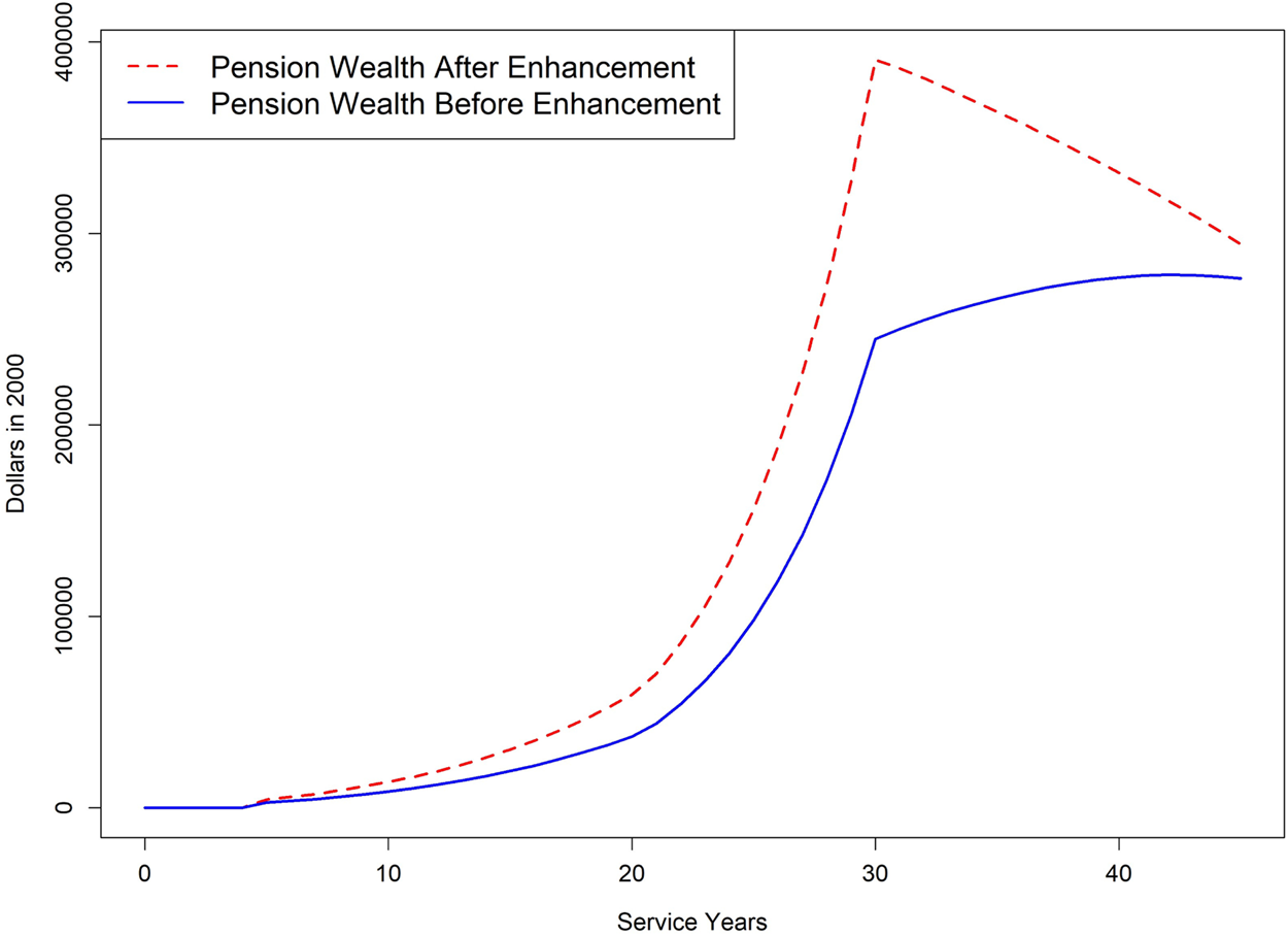
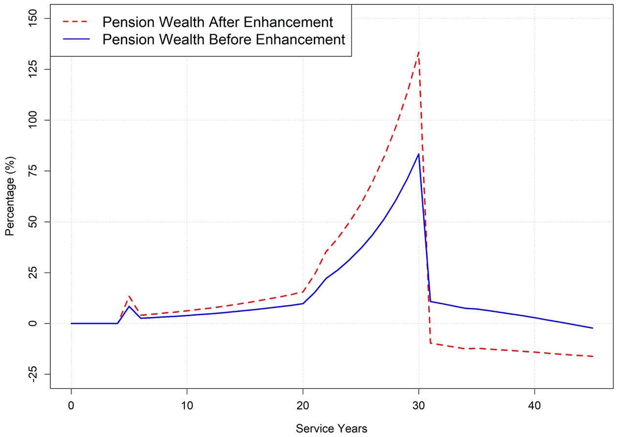
Figure 1 plots total pension wealth before and after pension enhancement for a representative teacher in St. Louis who enters the system at age 25 and works continuously until separation. Figure 2 plots annual pension wealth accrual before and after pension enhancement.
Accumulated pension wealth by service years for a teacher entering at age 25.
Note: The figure compares pension wealth accrual before and after the 1999 pension enhancements for a representative teacher in St. Louis who enters the system at age 25. For prediction of salary we use a cubic function of service years.

Annual changes in pension wealth for a teacher entering at age 25.
Note: The figure compares the pension wealth accumulation under the pension rules before and after the 1999 pension enhancements.

Figures 1 and 2 are consistent with the prior literature analyzing the ‘pull’ and ‘push’ incentives implied by different pension rules, e.g., Costrell and Podgursky (Reference Costrell and Podgursky2009). The steeply rising accrual up to peak value tends to lock in teachers, while the decline in pension wealth past the peak tends to push teachers in to retirement. What is notable in both figures is how much more powerful the ‘push’ incentives became after 1999. This is a direct result of the 60% of FAS annuity cap. Pension wealth accrued faster because of the sharp increase in the formula factor from 1.25% to 2.0%, and then declines sharply because of the 60% cap. The result is much more powerful incentives pushing our representative teacher into retirement around age 55.
3. Retirement behavior before and after pension enhancements
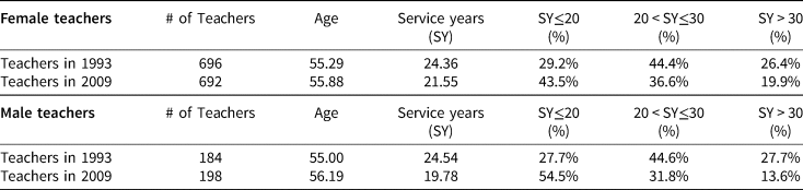
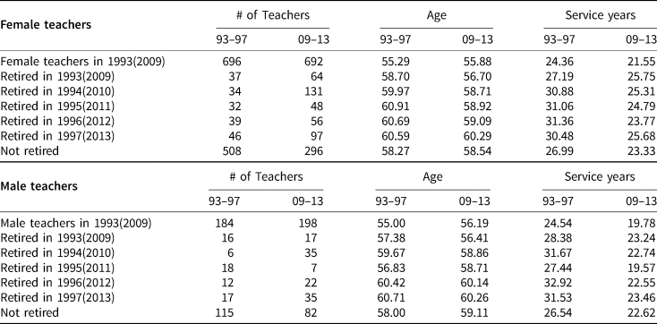
In this section we examine empirical retirement behavior before and after the 1999 pension enhancements. We use administrative data for St. Louis public school teachers and track two cohorts of teachers aged 50–62 at the beginning of the period forward for five years. The pre-enhancement cohort begins in Fall, 1992 and is followed to Fall, 1996, well before enactment or discussion of the 1999 changes. The post-enhancement cohort begins in Fall, 2008 and is tracked to Fall 2012. Again, this is well beyond the initial implementation of the enhancement. We have a cohort of 696 female and 184 male teachers in the 1993 cohort. By the end of the panel 186 females (27%) and 69 males (38%) had retired. The 2009 cohort had 692 female teachers and 198 male teachers of whom 396 female teachers (57%) and 116 male teachers (59%) had retired by the end of the panel. Tables 2 and 3 report the basic descriptive statistics in the base year and subsequent five years for the two cohorts.
Sample statistics in base year: before and after 1999 enhancements

Note: The table compares two cohorts of teachers aged 50–62 in the 1992–1993 and 2008–2009 school years in the base year. The age and service years columns report the averages for teachers. The last three columns report the bins of service years.
Sample statistics: before and after 1999 enhancements

Note: The table compares two cohorts of teachers aged 50–62 in the 1992–1993 and 2008–2009 school years. We track the two cohorts forward for five years. The age and service years columns report the averages for teachers in the base year, those who retired in each subsequent year, and who were not retired at the end of the sample period.
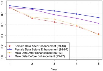
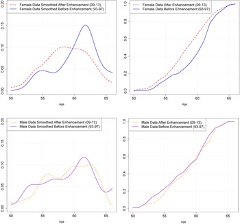
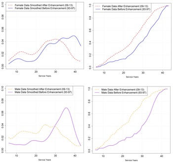
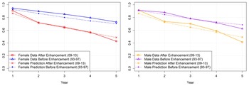
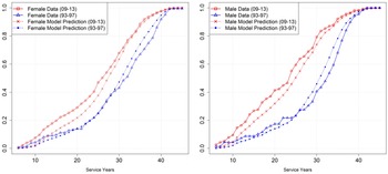
Table 3 suggests that teacher retirement behavior differs substantially under pre- and post-enhancement rules in two important ways. The first difference is that in the post enhancement period teachers retire earlier than in the pre-enhancement period. This is seen clearly in Figure 3 which reports the employment survival rates over five years. The post enhancement survival curve is well below the earlier cohort for both female and male teachers. Figures 4 and 5 report age and service years distributions of retired teachers in the two cohorts. Here it is important to note we only observe completed age and experience spells for teachers who have retired. Nonetheless, among the retirees, the cumulative age distribution is clearly displaced left for females. The results for males are somewhat more ambiguous. For both groups, however, there is a pronounced leftward displacement in the distribution of service years.
Employment survival rate before and after pension enhancements.
Note: The figure compares the employment survival rates for two cohorts of teachers (for female and male teachers) aged 50–62 at the base year and then tracks them for the next five years (93–97 and 09–13).

Age distribution before and after pension enhancements.
Note: The figure compares the age distributions for retired teachers (female and male teachers) before and after the 1999 enhancements. The teachers are aged 50–62 at the base year of two periods. The left graph compares the probability density, while the right graph compares the cumulative distribution. Please note that the figures are kernel-smoothed density estimates of data.

Service years distribution before and after pension enhancements.
Note: The figure compares the service years distributions for retired teachers (female and male teachers) before and after the 1999 enhancements. The teachers are aged 50–62 in the base year of the two periods. The left graph compares the probability density, while the right graph compares the cumulative distribution. The figures are kernel-smoothed density estimates.

It is also noteworthy that the average baseline service years of the senior teachers in the post-enhancement sample period is considerably lower than in the pre-enhancement sample, despite the fact that the average age is nearly identical. In 2009, at the beginning of the post-enhancement sample the female teachers are about 2.8 years less experienced than their same age-group counterpart in 1993, and male teachers in 2009 are about 4.8 years less experienced. This substantial difference in service years suggests in the post-enhancement sample teachers older than 50 tended to retire earlier (with fewer service years) due to the change in pension incentives. There are two implications of this observation. First, conditional on age, one would expect less experienced senior teachers to retire later, hence the earlier retirement by the post-enhancement cohort shown in Figures 4 and 5 is even more striking. Second, some teachers of age 50–62 are retirement-eligible prior to the beginning of the sample period. Their decision to stay on the job reflects preferences unobserved to the researchers. The distributions of these preferences are likely differ at the beginning of the pre- and post-enhancement periods because the pension rules themselves have reshaped the pool of senior teachers. This illustrates why it is important to take account of baseline sample selection in estimating a statistical retirement model. We will take up this issue of baseline sample selection when we discuss structural model estimation in the next section.
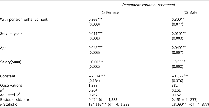
Before turning to modeling, we round out our empirical discussion by presenting simple regression-adjusted retirement rates for the two cohorts. Table 4 reports the results of fitting a simple linear probability model that predicts probability of retirement as a function of baseline age, service years, and whether a teacher is in the post-enhancement cohort. The coefficient on the post-enhancement cohort dummy implies that the probability of retirement, averaged over all age and service year cells was 37 percentage points higher for females, and 30 percentage points higher for males over the five-year period.
Regression estimates: linear probability models

Note: The table shows the results of linear probability model using the two cohorts of teachers in Table 3 in the base year.
Model: Retire i = β 0 + β 1Enhancement i + β 2ServiceYears i + β 3Age i + β 4Salary i + ɛ i;Dummy variable Retire = 1 if the teacher retired during the panel;Dummy variable With Pension Enhancement = 1 if the teacher is in the 09–13 cohort;*p<0.1; **p< 0.05; ***p<0.01. The standard errors are in parentheses.
The evidence in Tables 3 and 4 and Figures 3–5 suggests that the 1999 enhancements significantly shortened teaching careers and that the ‘push’ effects were very potent. To explore further the long-run effect of these changes on senior teachers, and consider how teachers would respond to alternate retirement plans, in the next section we estimate a structural model of retirement behavior and use it to examine the long-run effect of these rule changes on representative senior teachers.
4. Estimating a dynamic retirement model
Stock and Wise (Reference Stock and Wise1990) developed a structural model of retirement which was extended by Ni and Podgursky (Reference Ni and Podgursky2016) to an analysis of public school teachers. We apply this model, with several innovations, to an analysis of St. Louis teachers.
Consider an employed teacher who has not retired at the beginning of year t. The present value of expected lifetime utility for the teacher if she retires in year r (r ≥ t) is

where


The value function V depends on future annual earnings Y s before retirement, pension benefits P s(c 2) if the teacher starts collecting a pension benefit in year c 2, and Social Security benefits B s(c 1) if she starts collecting Social Security in year c 1. The collection years c 1 and c 2 are optimally chosen to maximize the expected utility given the retirement year r. The parameter c is the contribution rate for teachers before retirement, and k s represents the teacher's preference for teaching versus retirement, which, in turn, depends on the teacher's age in year s. We assume $k_s = k\left({{{60} \over {age}}} \right)^{k_1}$ . The errors ω s and ξ s measure preferences for teaching and retiring, respectively. The conditional survival rate π( s|t ) is based on U.S. mortality data.
The expected gain from postponing retirement to year r is

Each year, an employed teacher has two choices: continue teaching or retire. The expected gain from postponing retirement can be seen as the ‘option value’ of continuing to work, which is a key feature of this model. Retirement occurs if the value of continuing teaching is less than the value of retiring, i.e., the option value of continued teaching is negative.
The teacher's future salary, pension benefits, and Social Security benefits are assumed to be predictableFootnote 3. We know the salary of teachers in the first period and then we predict the future salary with forecasts based on historical data.
The expected gain from retiring in year r (later than t) is

where the first term $g_t( r ) \! = \!\mathop \sum_{s = t}^{r-1} \beta ^{s-t}\pi ( {s\vert t} ) \;( {{( {k_s( {( {1\! - \!c} ) Y_s \! + \! I_s^1 B_s( {c_1} ) } ) } ) }^\gamma } ) + \mathop \sum_{s = r}^{T} \beta ^{s-t}\pi ( {\mkern 1mu} s\vert t{\mkern 1mu} ) {\mkern 1mu} ( ( I_s^2 P_s( c_2)\,+$ $ I_s^1 B_s( c_1) ) ^\gamma -\left[{\mathop \sum \nolimits_{s = t}^{T} \beta^{s-t}\pi ( {\;s\vert t\;} ) \;{( {I_s^2 P_s( {c_2} ) + I_s^1 B_s( {c_1} ) } ) }^\gamma } \right]$
 , depends on pension rules. The second term, $K_t( r ) = \mathop \sum \nolimits_{s = t}^{r-1} ( {\beta \rho } ) ^{s-t}\pi ( {\;s\vert t\;} )$
 , depends on the mortality rates. Both terms depend on the parameters we need to estimate. The preference error ν t = ω t − ξ t. We assume ν t follows an AR(1) process: ν t = ρν t−1 + ɛ t, where ɛ t is iid N(0, σ 2).
Suppose $r^{\dagger}$ solves max r∈{t+1,t+2,……T} $\opf E$
 tV t(r). Thus, the teacher will continue working at t if $G_t( {r^{\dagger} } ) = {\rm {\opf E}}_tV_t( {r^{\dagger} } ) -{\rm {\opf E}}_tV_t( t ) > 0$
 . The probability of retirement at time t is $P[ {R = t} ] = P[ {G_t( r ) \le 0, \;\forall r \ge t + 1} ] = P[ {G_t( {r^{\dagger} } ) \le 0} ] , \;$
 which can be rewritten as

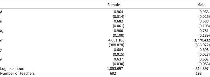
In this model there are six unknown structural parameters to be estimated, which are listed in Table 5. The threshold $g_t( {r_t^{\dagger} } ) {\rm /}K_t( {r_t^{\dagger} } )$ depends on teacher's age, service years, and the six structural parameters. Details concerning the computation of the retirement probabilities are given in Appendix A.1.
Structural model parameters

The structural model assumes that retirement decisions by teachers are governed by the six parameters. Teachers with the same age and service years differ in timing of retirement due to differences in preference errors ν t that measure the unobserved willingness to teach (relative to retirement). The preference errors are partly endogenous because they depend on teachers' past retirement decisions. Condition (8) implies that the preference errors ν t for teachers who choose to continue teaching are greater than ${-}g_t( {r_t^{\dagger} } ) {\rm /}K_t( {r_t^{\dagger} } )$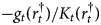 . Teachers with above average age and service years and who repeatedly choose to remain working imply higher values of ν t. In the model estimation we factor in the dependence of the thresholds on preference errors by computing the sequential probabilities of the teachers' decisions.
The dependence of the preference errors pertains to the initial sample as well as the panel and results in the baseline sample selection problem noted in the previous section. The estimation data set includes teachers who were eligible for retirement before 2008 (the beginning of sample period) but who chose to wait, but it excludes those who chose to retire prior to 2008. Failing to take this sample selection into account would result in biased estimates. Hence, the sample selection in this setting is an example of the familiar ‘initial condition problem’ in dynamic panel data models (e.g., Heckman, Reference Heckman, Manski and McFadden1981; Wooldridge, Reference Wooldridge2005).
We solve the ‘missing early leavers’ problem by estimating the model conditioning on the probability that retirement-eligible teachers appear in the initial sample. The option-value model depicts how the sample selection depends on the preference errors prior to the initial sample period.
The likelihood of the sample can then be computed by integrating out these baseline preference errors along with the preference errors in the sample period. Our approach to correcting this sample selection problem is discussed in greater detail in Appendix A.2.
The data we use for estimation includes all teachers aged 50–62 in the 2008–2009 school year, which is the cohort of teachers under the post-enhancement pension rules described in Table 3. We track this cohort of teachers for the next five years. Using maximum likelihood estimation (MLE) methods described in the Appendix, we obtain the estimates of six structural parameters reported in Table 6.
Estimates of structural parameters

All of these parameter estimates are statistically significant, plausible, and estimated with reasonable to high precision. Compared with the estimates in Ni and Podgursky (Reference Ni and Podgursky2016), these ‘deep’ parameters, i.e., capturing basic preferences, are quite similar even though the St. Louis teachers are in a separate and substantially different FAS-DB pension system. In addition, St. Louis teachers are covered by Social Security, whereas teachers in the state-wide plan are not.
The parameter β measures the teacher's discount rate. The parameter γ is significantly less than unity for both female and males, which implies risk-aversion. σ and ρ are two parameters related to unobserved retirement preferences. These unobserved preferences (‘preference shocks’) are substantial and persistent (i.e., ρ is positive and significant). Since the option value is the key variable in this model that predicts retirement behavior, the large standard deviation estimates of 4,001.108 and 3,770.432, for females and males, respectively, are reasonable since they capture all other omitted variables that influence retirement decisions. The parameters k and k 1 together measure the disutility of teaching relative to retirement. These estimates imply that the attractiveness of retirement (leisure) relative to teaching rises with age (Ni and Podgursky, Reference Ni and Podgursky2016).
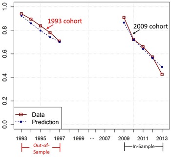
The structural model provides a good fit to these data both in and out of the sample. Figure 6 reports employment survival rates in-sample for the 2009 senior teacher cohort and out-of-sample for the 1993 cohort. Note that the 1993 out-of-sample cohort is a non-overlapping group of teachers who face a very different set of pension rules. Nonetheless, the fit is good for both groups. More extensive plots of age and service years are provided in Appendix B. Overall, the structural model exhibits good fit, both in and out-of-sample.
Observed and predicted survival rate for all teachers (in sample and out of sample).
Note: The figure compares the observed and predicted survival rate of two cohorts of teachers: in-sample (2009 cohort) and out-of-sample (1993 cohort) teachers. Male and female teachers are pooled.

5. Simulating the effects of pension plan changes
As noted in the introduction, the 1999 enhancement of the replacement factor was accompanied by a cap on pension benefits of 60% of final average salary. Using the estimated structural model we conduct counter-factual simulations on the effect of each aspect of the pension rule changes.
In order to remove the influence of the composition of teachers in the post-enhancement sample and highlight the policy effect, we choose a representative female and male teacher who is 50 years old and with 25 years of service. Such a teacher is entering the retirement window. We analyze the effects of the pension enhancements and three counterfactual pension alternatives over a 30-year time horizon, by which time this teacher will have retired.
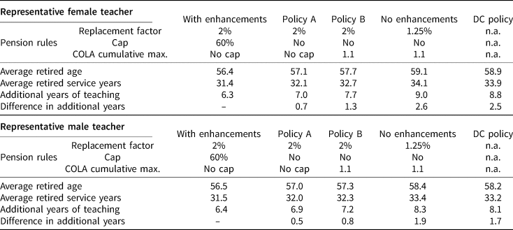
Table 7 reports the effects of the different pension rules on the timing of retirement. We treat the after-enhancement pension rules as our baseline case (column 2) and subtract enhancement effects. Column 5 reports the effect of eliminating all of the enhancements. The elimination of pension cap of 60%, a reduction of 0.75% in the replacement factor, and a COLA cap leads to a higher level of average retirement age and extends the teaching career by 2.6 years for females and 1.9 years for males. This shows that the less remunerative and uncapped pre-enhancement pensions exerted a weaker ‘push’ effect, and hence yielded longer teaching careers.
Effects of alternative pension rules on a representative senior teacher

Note: The simulation tracks a representative female and male teacher aged 50 with 25 years of service for the next 30 years under four cases: a baseline with enhancements; Policy A eliminates the pension cap of 60%; Policy B further imposes the maximum increase of 10% on the retirement COLA adjustment; before-enhancement policy; DC Policy with investment returns of 4%. Additional teaching years is the number of years the teacher is expected to teach before retirement. Difference in additional teaching years is the additional teaching years under an alternative policy minus that under the baseline DB policy (with the enhancements in place). The DC plan assumes that teachers contribute 5% and the district contributes 10% of salary.
Table 7 also decomposes the effects of the pension enhancements into the components due to increasing the replacement factor and the effect of a benefit cap. Eliminating the cap on pension benefits increases the average service years at retirement by 0.7 years for female teachers and 0.5 years for male teachers. Imposing the COLA cap increases service years of retirement from 0.3 to 0.6 years. Reducing the replacement factor from 2% to 1.25% increases the average service years of retirement by 1.3 years for female and 1.1 years for male teachers.
In short, the somewhat surprising finding from Table 7 is that while the 60% cap, which has a clear ‘push’ effect, shortened teaching careers, the larger effect came from the increase in the replacement factor from 1.25% to 2%. The COLA cap also had a potent effect.
Over the last several decades many private sector employers have frozen or closed their DB plans and put workers into DC plans (Butrica et al., Reference Butrica, Iams, Smith and Toder2009). Several papers in the retirement literature have used reduced form and structural estimates of retirement behavior of employees in DB plans to simulate what the effect of retirement behavior under an alternative DC plan (e.g., Friedberg and Webb, Reference Friedberg and Webb2005; Costrell and McGee, Reference Costrell and McGee2010; Ni and Podgursky, Reference Ni and Podgursky2016; Ni et al., Reference Ni, Podgursky and Wang2020). In part this is necessitated by the fact that an involuntary conversion of state and local employees (including teachers) to a DC is illegal under state constitutions (Monahan, Reference Monahan2010). Thus, the only such conversions to date have been for newly hired public sector employees whose retirement behavior will not be observed for many years to come. A DC plan, while clearly a major change from the DB plan on which we base our estimates, may not be too far ‘out of sample’ to justify simulating its workforce effects. In the context of our model, the major difference between DB and DC is that the latter removes all ‘push’ incentives.Footnote 4 In this respect it mirrors in reverse the powerful push incentives introduced in 1999 – i.e., an increase in the replacement rate from 1.25% to 2.0% combined with a 60% benefit cap.
With these caveats in mind, the final column of Table 6 simulates the effect of a DC conversion for St. Louis teachers. This plan would freeze accrual of pension wealth under the current DB plan and convert all future contributions toward a less expensive (but still generous by private sector standards) DC plan. Specifically, the teacher would receive the full value of her accrued pension wealth. We assume a 4% annual nominal return on this balance. Going forward, the teacher would contribute 5% of her salary to the DC plan (which matches her contribution rate to the DB plan) and the district would contribute 10%. The district contribution rate is less than the current cost of the DB plan.
The last column of Table 7 shows the behavior of our representative senior teacher under such a hypothetical DC plan. The mandatory conversion to a DC plan produces a substantial increase in additional teaching years and retirement age. As compared to the current plan, completed service years at retirement rises by 2.5 and 1.7 years for females and males, respectively. Average age at retirement rises from 56.4 to 58.9 for females and 56.5 to 58.2 for males. These substantial increases from a DC conversion are robust to modest changes in underlying assumptions regarding returns or contribution. This exercise highlights the potent effect of the ‘push’ incentives built into both the current and pre-enhancement DB plans. A DC conversion neutralizes the ‘push’ and thus substantially extends a teaching career.Footnote 5
Of course, a mandatory conversion to DC may reduce the welfare of late-career teachers who are far from reaching the pension wealth peak. As a consequence such a mandatory conversion would almost certainly be unconstitutional in most states (Monahan, Reference Monahan2010). However, some states that have implemented hybrid plans (combined DB and DC) for new hires have permitted more senior to teachers to voluntarily opt into the new plan (e.g., Goldhaber and Grout, Reference Goldhaber and Grout2016). In unpublished simulations, we find that if faced with a voluntary DC conversion option (even at rates of conversion between 80% and 90% of full pension wealth), many male and female teachers at or near peak value opt for a conversion. Teachers below the peak value in service years may also opt for the conversion, but their probability of accepting the conversion is much more sensitive to the terms of the offers than that of teachers near peak value. At a minimum, dynamic structural models can provide rough empirical estimates of the take up rates for buyout or conversion options.
6. Conclusion
Many states enhanced benefits in teacher retirement plans during the 1990s. This paper examines the effect of a major enhancement for teachers in St. Louis public schools in 1999. Pension rule changes in 1999 resulted in very large increases in pension wealth for active teachers, as well as a powerful increase in ‘push’ incentives for earlier retirement. Simple descriptive statistics on retirement patterns before and after the enhancements suggest earlier retirement. However, to better understand the long-run effects of these changes, we estimated a structural retirement model using panel data for the St. Louis teachers. Simulations based on the structural estimates imply shorter completed teaching spells and earlier retirement ages for a representative senior teacher as a result of the enhancements. These shorter teaching spells imply a steady state with more teacher turnover and a larger share of novice teachers in classrooms. A large teacher value-added literature finds that novice teachers (e.g., teachers with less than three years teaching experience) are less effective in raising student achievement (e.g., Clotfelter, Ladd, and Vigdor, Reference Clotfelter, Ladd and Vigdor2006; Wiswall, Reference Wiswall2013). The latter would imply lower overall workforce quality. When combined with the Koedel and Xiang (Reference Koedel and Xiang2017) finding that the large St. Louis teacher enhancements had little effect on retaining younger teachers, this would seem to call into question the efficacy of such a back-loaded compensation policy.Footnote 6
By contrast, conversion to a less expensive DC type plan, which eliminates the ‘push’ incentives into retirement, would substantially lengthen expected teaching careers for senior St. Louis teachers. A mandatory conversion to a DC plan would substantially extend expected teaching careers among senior teachers. A study of Tennessee teachers (Ni et al., Reference Ni, Podgursky and Wang2020), who are covered by a similar DB retirement plan, finds substantial improvement in the quality of the senior workforce, along with a lengthening of teaching careers in simulated conversations to a DC type plan. Our simulations also suggest that many senior teachers would opt into a voluntary DC plan as well.
This paper has focused on the retirement behavior of senior teachers. We have not attempted to model the effect of pension plan changes on younger teachers or recruitment. As noted, Koedel and Xiang (Reference Koedel and Xiang2017) find little effect of the large pension enhancements on the short-term turnover behavior of younger teachers. However, it is possible that fundamental changes to the plan itself, such as partial or total conversion to DC, would affect recruitment into the profession and early career turnover. While young teachers do display little knowledge of the specifics of their retirement plans, there is some evidence that they would prefer a DC type plan (e.g., Goldhaber and Grout, Reference Goldhaber and Grout2016; DeArmond and Goldhaber, Reference DeArmond and Goldhaber2010). However, recruitment and early career retention effects of fundamental plan redesign are beyond the scope of this study.
As a post-script to this study, rising pension plan costs and growing unfunded liabilities have led plan administrators and school leaders to cut retirement benefits for new St. Louis teachers (hired in 2018 or later) and raise contribution rates for new teachers from 5 to 9% of salary. However, it will be many years before these newly hired teachers are eligible for retirement. In the meantime, the pension incentives described in this paper will be shaping retirement incentives, and shortening teaching careers of incumbent teachers for many years to come. The structural methods used in this paper can help policy makers better understand the short- and long-run staffing and fiscal consequences of the ongoing changes in pension plan design.
Acknowledgements
This research was supported by the National Center for the Analysis of Longitudinal Data in Education Research (CALDER), which is funded by a consortium of foundations. For more information about CALDER funders, see www.caldercenter.org/about-calder. The authors also acknowledge support from the Charles Koch Foundation. All opinions expressed in this paper are those of the authors and do not necessarily reflect the views of our funders or the institutions to which the author(s) are affiliated. CALDER working papers have not undergone final formal review and should not be cited or distributed without permission from the authors. They are intended to encourage discussion and suggestions for revision before final publication. We also thank the editor and two referees for insightful comments and suggestions.
Appendices
Appendix A – Statistical appendix
A.1 Numerical computation of retirement probability
Continuing with the notation from Section 4, denote $f_t^ {\dagger} { = } g_t( {r^ {\dagger} } ) {\rm /}K_t( {r^ {\dagger} } )$ . Suppose year 1 is the first year of our sample period, and year N is the last year of the sample period. Denote $V_{t_1, t_2} = ( {\nu_{t_1}, \;\ldots , \;\nu_{t_2}} )$
 , $F_{t_1, t_2}^ {\dagger} { = } ( {f_{t_1}^ {\dagger} , \;\ldots , \;f_{t_2}^ {\dagger} } )$
 . The unconditional likelihood (unconditional probability) that teacher i chooses to retire at year n (n < N) is

The unconditional probability that teacher i chooses to stay until year N is

These probabilities depend on pension rules, teachers' age and service years, and structural parameters (γ, k, k 1, β, σ, ρ). Under the normality assumption of preference errors, computing the probabilities for the retirement decision made by teacher i involves a high-dimensional numerical integration of the correlated preference errors V over the region A i, for which we use the Geweke–Hajivassiliou–Keane (GHK) algorithm. The GHK algorithm transforms the problem of high-dimensional integration to a problem of sequential one-dimensional integrations. For more applications of the GHK algorithm see, for example, Börsch-Supan and Hajivassiliou (Reference Börsch-Supan and Hajivassiliou1993).
A.2 Censoring in the baseline sample
The sample excludes those teachers whose age and service years would have put them in our sample but who chose to retire before our sample period. This results in sample selection bias. Sample selection bias of this sort will lead to overprediction of retirement for relatively young teachers (Ni and Podgursky, Reference Ni and Podgursky2016). We correct for sample selection bias in our baseline sample by using conditional probability to construct the likelihood function. The probability of teachers retiring in our sample period is based on the condition that teachers are not retired at the beginning of the sample period.
Suppose in the first year of our sample period, teacher i was eligible for retirement J years ago. The probability of teacher i retiring at time n < N conditional on being in the sample is


The conditional probability of teacher i chooses to stay until the end of sample period N is


Given the observations of teachers i = 1, …, I who retired during the sample period (at n i < N) or not retired until the end of the sample period (n i = N), the conditional likelihood for the whole sample is

We use the likelihood in equation (A.3) to estimate our structural model.
Appendix B – Goodness of fit
B.1 In-sample goodness of fit
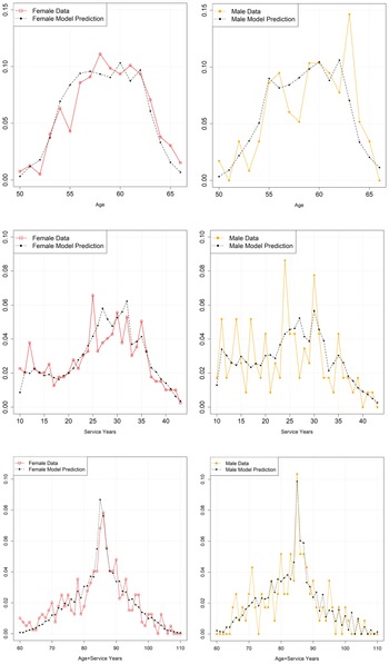
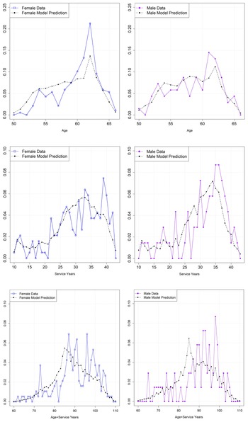
Figure B1 reports the observed and predicted distributions of age, service years, and the sum of age and service years for retired teachers. There is a sharp spike at 85 and 86 reflecting the ‘Rule of 85’ (i.e., age + service years = 85) option for regular retirement.
Observed and predicted retired age, service years and age + service years distribution of female and male teachers (In sample).

While the observed age and service years distributions are somewhat choppy because of the relatively small sample sizes (particularly for male teachers), overall they are in line with the predicted distributions. All the above figures show that the model nicely mimics the distribution of both age and service years, in particular the ‘Rule of 85’.
B.2 Out-of-sample goodness of fit
The out-of-sample simulation provides a robust check for the validity of our model. The data we use for out-of-sample simulation include all teachers aged 50–62 in the 1993–1997 school year. The basic statistics are shown in Table 3. The table shows that under different rules the patterns of retirement rates differ before and after the enhancement as well as the distributions of teacher service years at the time of retirement. Using the estimated parameters in Table 6, we simulate the teachers retirement behaviors in 1993–1997 school years. During this period, the teachers are under pre-enhancement pension rules. The out-of-sample simulation also takes into account of the fact that teachers in 1993 are significantly different from those in 2009 in age and service years. Figure B2 reports the observed and predicted distribution of age, service years, and the sum of age and service years for retired teachers for the out-of-sample simulation.
Observed and predicted retired age, service years and age + service years distribution of female and male teachers (out of sample).

B.3 Overall goodness of fit
Figure B3 provides both the in-sample and out-of-sample goodness of fit of the survival rate. Figure B4 plots the observed and predicted in- and out-of-sample cumulative distributions of service years at the time of retirement. Overall, the model with the same parameters in teacher preference can capture the difference in retirement patterns for teachers under different pension rules.
Observed and predicted survival rate (in sample and out of sample).

Observed and predicted retired service years cumulative distribution of female and male teachers (in sample and out of sample).

Appendix C – DC analytics
If in year t a teacher with age-experience (a, e) plans to retire in year r ≥ t, her expected utility under the DB plan is denoted as ${\rm {\opf E}}_tV_t^{DB} ( r )$ in equation (1). We use a similar notation for the expected utility under the following DC plan.
A teacher with (age,experience) (a, e) in the DB plan in a base year has cash balance W(a, e). Going forward, the value in this account grows by the nominal interest rate (on the fund balance) and further annual contributions from teachers and districts of c t and c d fraction of salary for teachers and districts, respectively, for a combined total of c t + c d times salary. A teacher's account accumulates with annual contributions and nominal investment returns of R − 1 on the fund balance. The inflation rate is assumed to be i.
The teacher considers whether to retire or continue to work as in the SW model: her expected utility in period t is a function of expected retirement year r (with r = t, ⋅ ⋅ ⋅ , T and T = 101 is an upper bound on age). For a teacher with a DC account value W t = W(a, e), the account nominal value in year r > t is the value of accumulation of contributions plus the compound return of the wealth in period t: $W_r = W_tR^{r-t} + \mathop \sum \nolimits_{k = t + 1}^r ( {c_t + c_d} ) Y_kR^{r-k}, \;$ Y k is salary in year k.
When a teacher retires, the contribution to the account stops and an insurance company provides an actuarially fair annuity (B) equal to the cash value in the teacher's account.
For a teacher with a DC account value W r, age a + (r − t) at the time of retirement (the teacher's age is a in year t), let the expected nominal flow of the annuity be B r+n in the n −th year of retirement. The retiree survives to r + n with conditional probability π(r + n|r). The expected account value and the expected payment evolve from the collection r as

We set W T = 0. It follows that given age a + (r − t) at the time of retirement has DC benefit

The benefit in time t dollar is B r(DC) = B r(1 + i)r−t.
In period t, the expected utility of retiring in period r under the DC plan, ${\rm {\opf E}}_tV_t^{DC} ( r )$ , is the discounted sum of pre- and post-retirement expected utility after replacing the DB annual benefit in equation (1) by the DC annuity B r(DC).