


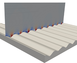

1. Introduction
Oscillatory turbulent motion is encountered in a number of engineering, biological and environmental flows. For instance, the seabed in coastal zones is characterized by the oscillatory motion generated by free-surface gravity waves. The so-called wave bottom boundary layer that forms as a result affects the whole seabed ecosystem, from remodelling the bed morphology (sediment erosion, transport and deposition) to the transport of nutrients and substances dispersed in water.
Oscillatory wall bounded flow is a relatively well studied problem in fluid mechanics. One of the few known analytical solutions of the Navier–Stokes equations is the so-called Stokes’ second problem (Batchelor Reference Batchelor1967; Schlichting Reference Schlichting1979), which describes the laminar flow generated by a flat plate oscillating harmonically in its own plane and bounding a fluid otherwise at rest. The solution was given by Stokes (Reference Stokes1851) and shows that the oscillatory motion propagates by viscous action from the wall to the bulk of the fluid up to a distance  $\delta$, depending on the fluid and the frequency of the oscillations. Observing the fluid from a reference frame fixed with the plate, the motion has the character of an oscillating boundary layer, driven by the shear at the bottom wall. Later, Lamb (Reference Lamb1933) calculated the solution for the case of a flat plate at rest bounding a fluid forced by a harmonic pressure gradient. In this case, since the bed is a smooth flat plate, there are no inertial effects different from the oscillating plate problem. Thus the pressure-driven solution coincides with the Stokes shear-driven flow with axes fixed on the plate.
The analogy of the shear-driven flow with the pressure-driven case has been leveraged by some early experimental works on the wave bottom boundary layer and sediment transport (Bagnold Reference Bagnold1946; Manohar Reference Manohar1955). For example, in his seminal work, Bagnold (Reference Bagnold1946) disposed layers of sediments on a tray oscillated by a motor, inducing in this way a shear-driven boundary layer in otherwise still water. In coastal zones, the bottom boundary layer is rather pressure-driven because of the free-surface gravity waves. The laboratory configuration that more closely reproduces field conditions is thus a wave flume. However, these systems may require prohibitively large facilities to achieve realistic wave heights and periods (Komar & Miller Reference Komar and Miller1973) and avoid wave-breaking issues (Mirfenderesk & Young Reference Mirfenderesk and Young2003), and have thus seen wide application only in more recent times (Mirfenderesk & Young Reference Mirfenderesk and Young2003; Nichols & Foster Reference Nichols and Foster2007; Rodríguez-Abudo, Foster & Henriquez Reference Rodríguez-Abudo, Foster and Henriquez2013; Rodríguez-Abudo & Foster Reference Rodríguez-Abudo and Foster2014). A large body of experimental measurements has been obtained with oscillating tray rigs (such as the shear-driven set-up used by Bagnold (Reference Bagnold1946) and several other authors: Li Reference Li1954; Manohar Reference Manohar1955; Kalkanis Reference Kalkanis1957; Sleath Reference Sleath1976; Young & Sleath Reference Young and Sleath1990) or oscillatory flow water tunnels (Jonsson & Carlsen Reference Jonsson and Carlsen1976; Sato, Mimura & Watanabe Reference Sato, Mimura and Watanabe1984; Sleath Reference Sleath1988; Smith & Sleath Reference Smith and Sleath2005; Admiraal et al. Reference Admiraal, Musalem-Jara, García and Niño2006), in which water oscillates to and fro over a stationary bed within the tunnel section in response to a pressure-driven piston forcing.
There has been relatively limited attention to compare the two types of forcings beyond the equivalency established by the laminar flow solutions of Stokes and Lamb for a smooth flat plate. In coastal environments, the bed is not flat, and the flow is turbulent rather than laminar (Blondeaux Reference Blondeaux2001). A few early studies (Komar & Miller Reference Komar and Miller1973, Reference Komar and Miller1975) surveyed literature data from both oscillatory tray rigs and oscillatory water tunnels, reporting a good agreement between shear-driven and pressure-driven estimates of an equivalent Shields parameter for sediment motion initiation, while some discrepancies were observed on the critical Reynolds number for laminar–turbulent transition. As later reported by Sleath (Reference Sleath1988), a scatter in the transitional Reynolds number is also observed among other pressure-driven (Vincent Reference Vincent1957; Lhermitte Reference Lhermitte1958) and shear-driven (Li Reference Li1954; Manohar Reference Manohar1955) data from studies over flat rough beds. However, the magnitude of the discrepancy does not appear large enough to exclude the impact of other uncertainties arising in the comparison (Sleath Reference Sleath1988).
When the bed is relatively rough or has large-scale ripples, the exposed bed surface will be subject to a large form drag because of the external pressure gradient. This component of the bed drag cannot be reproduced in oscillating tray configurations, where the pressure gradient is zero (Sleath Reference Sleath1991). In discussing the analogies between oscillatory flows and non-periodic acceleration/deceleration, Scotti & Piomelli (Reference Scotti and Piomelli2001) pointed out that a non-uniform (i.e. variable in space) time-varying pressure gradient cannot be reduced with a transformation of variables to a time-varying boundary condition as for the classic Stokes and Lamb laminar solutions. Thus in a rippled bed, where such local pressure variations are to be expected, larger discrepancies could result between the two types of forcings. Du Toit & Sleath (Reference Du Toit and Sleath1981) investigated oscillatory flow over rippled beds using both an oscillatory-tray apparatus and an oscillating water tunnel. However, they were unable to investigate the same range of flow conditions in both configurations, because of the operative specifications of each system. More detailed comparisons of the flow in the boundary layer for these different forcings are scarce, partly because of inevitable limitations in available experimental facilities. Nonetheless, the use of oscillating trays to investigate bottom boundary layer dynamics has not ceased (see, for example, the recent works of Hay et al. Reference Hay, Zedel, Cheel and Dillon2012; Hare et al. Reference Hare, Hay, Zedel and Cheel2014; Aponte Cruz & Rodríguez-Abudo Reference Aponte Cruz and Rodríguez-Abudo2024).
A number of numerical studies have been performed to study the flow over rippled beds, from the early two-dimensional numerical calculations (Sleath Reference Sleath1975; Longuet-Higgins Reference Longuet-Higgins1981; Smith & Stansby Reference Smith and Stansby1985; Blondeaux & Vittori Reference Blondeaux and Vittori1991), to more recent large-eddy and direct numerical simulations (Scandura, Vittori & Blondeaux Reference Scandura, Vittori and Blondeaux2000; Barr et al. Reference Barr, Slinn, Pierro and Winters2004; Blondeaux, Scandura & Vittori Reference Blondeaux, Scandura and Vittori2004; Grigoriadis, Dimas & Balaras Reference Grigoriadis, Dimas and Balaras2012; Penko et al. Reference Penko, Calantoni, Rodríguez-Abudo, Foster and Slinn2013; Leftheriotis & Dimas Reference Leftheriotis and Dimas2016; Önder & Yuan Reference Önder and Yuan2019; Chalmoukis, Dimas & Grigoriadis Reference Chalmoukis, Dimas and Grigoriadis2020), providing additional insights on the flow and bed mechanics. Nonetheless, these studies have exclusively employed an oscillatory pressure forcing, which mimics more closely field conditions and is relatively more straightforward to implement numerically. There is a lack of accurate comparison between shear-driven and pressure-driven oscillatory flows, which is the goal of this paper. This study is conducted using direct numerical simulations, with the immersed boundary method to model the bed geometry. An external sinusoidal pressure gradient is used to reproduce the pressure-driven flow over the ripples. The shear-driven case is reproduced setting the external forcing to zero and changing the boundary condition at the bed from no-slip to a prescribed sinusoidal velocity. The simulation configuration (rippled bed and oscillation parameters) reproduces conditions from an oscillatory-tray apparatus. Available particle image velocimetry data from the experiment thus provide a benchmark for the shear-driven oscillatory boundary layer. The reader is referred to Vargas-Martinez & Rodríguez-Abudo (Reference Vargas-Martinez and Rodríguez-Abudo2024) for a detailed presentation and discussion of the experimental results.
The remainder of the paper is organized as follows. The details of the numerical methodology and the flow configuration are described in § 2. The analysis of the results is reported in § 3, and conclusions are summarized in § 4.
2. Methodology
The governing equations are the incompressible, non-dimensional continuity and Navier–Stokes equations:
 \begin{equation} \frac{\partial U_i}{\partial x_i} = 0, \end{equation}
 \begin{equation} \frac{\partial U_i}{\partial t } + \frac{\partial}{\partial x_j}\left(U_i U_j\right) ={-}\frac{\partial p}{\partial x_i} + \frac{1}{{{Re}}}\,\frac{\partial^2 U_i}{\partial x_j\,\partial x_j} + \varPi\delta_{i1}, \end{equation}
where  $U_i$ is the component of the velocity vector in direction
 $x_i$ (
 $i = 1$, or
 $x$, streamwise direction;
 $i=2$, or
 $y$, spanwise direction; and
 $i=3$, or
 $z$, wall-normal direction),
 $p$ is the pressure,
 $\delta _{ij}$ is the Kronecker delta. Also,
 ${{Re}} = U_0 \delta /\nu$ is the Reynolds number based on the amplitude of the oscillatory motion
 $U_0$, the Stokes’ layer depth
 $\delta = \sqrt {2\nu /\omega }$, and the fluid kinematic viscosity
 $\nu$. Amplitude
 $U_0$ and angular frequency
 $\omega$ are set to match the experimental conditions:
 $U_0 = 0.31\,{\rm m}\,{\rm s}^{-1}$, and
 $\omega = 2{\rm \pi} /T \approx 1.257\,{\rm rad}\,{\rm s}^{-1}$ (where
 $T = 5\,{\rm s}$ is the period of the oscillations). This results in a Reynolds number
 ${{Re}} = 390$.
In (2.2),  $\varPi$ is a uniform (i.e. constant in space) externally applied pressure gradient applied in the streamwise direction
 $x_1$ (which adds to the local term
 $\partial p/\partial x_i$ computed directly as part of the solution of the Navier–Stokes equations). For the pressure-driven case, the external pressure gradient is set to
 \begin{equation} \varPi ={-}\frac{\omega\delta}{U_0} \cos\omega t \end{equation}
together with a no-slip boundary condition  $U_i\equiv 0$ on the lower wall (the rippled bed). The oscillating pressure gradient in (2.3) leads to a free stream oscillating as
 $U_0 \sin \omega t$.
In the shear-driven case, the external pressure gradient is set to zero ( $\varPi = 0$), and the boundary condition on the lower wall is set to
 \begin{equation} U_i\left(x,y,z=z_{bed},t\right)={-} U_0\delta_{i1} \sin\omega t, \end{equation}
where  $z_{bed}(x)$ is the rippled bed waveform (figure 1a). Thus in a reference frame moving with the bed, the free-stream motion is the same as the pressure-driven case,
 $U_0\sin \omega t$.
Configuration. (a) Rippled bed waveform, with definitions of ripple parameters, wavelength  $\lambda$ and amplitude
 $k$. Also shown is the particle image velocimetry (PIV) field of view of the experimental dataset. (b) Three-dimensional view of the computational domain.

The other boundary conditions are the same for both the shear-driven and pressure-driven set-ups. Periodicity is applied in the  $x$ and
 $y$ directions, and free-slip is applied at the top boundary of the domain. The lower boundary of the domain consists of a rippled bed (figure 1). The bedform is approximately sinusoidal with average wavelength
 $\lambda = 7.73\,{\rm cm}$ and amplitude
 $k=1.8\,{\rm cm}$ (see inset in figure 1 for the definitions). This results in a Keulegan–Carpenter number
 $KC = 2{\rm \pi} A/\lambda \approx 20$ (where
 $A = U_0/\omega$ is the wave orbital amplitude). The bedform replicates the rigid bed placed over the oscillating cart in the experimental reference (Aponte Cruz & Rodríguez-Abudo Reference Aponte Cruz and Rodríguez-Abudo2024; Vargas-Martinez & Rodríguez-Abudo Reference Vargas-Martinez and Rodríguez-Abudo2024). The computational domain in the streamwise direction (
 $x$) fully includes the original ripple waveform, and has length
 $3\lambda$, as shown in figure 1(b). In the spanwise direction, the width has been taken equal to
 $3\lambda$, and
 $1.66\lambda$ in the bed-normal direction. The grid consisted of
 $768\times 256\times 768$ grid points in the streamwise, spanwise and bed-normal directions, respectively. The grid points are distributed uniformly in the
 $x$–
 $y$ plane, while stretching is applied in the
 $z$ direction to cluster more points close to the ripples:
 $640$ points are distributed uniformly within a layer of height
 $1.2\lambda$ from the lowest trough of the ripples (
 $z=0$ plane). In terms of Stokes layer depths, the resolutions in the bed-parallel directions (
 $x$ and
 $y$) are
 $\Delta x = 0.24\delta$ and
 $\Delta y = 0.74\delta$. In the
 $z$ direction, near the bed the resolution is
 $\Delta z \approx 0.094\delta$, i.e. approximately
 $10$ grid points per Stokes layer thickness, or approximately
 $4$ wall units (
 $\Delta z\, u_{\tau,0}/\nu$, based on the mean absolute friction velocity over the cycle
 $u_{\tau,0}$). More details and results of a grid sensitivity study are reported in Appendix A.
The bed is treated with the immersed boundary method described in Orlandi & Leonardi (Reference Orlandi and Leonardi2006). The numerical discretization, discussed in detail in Orlandi (Reference Orlandi2000), employs the centred second-order finite-difference approximation on an orthogonal staggered grid. The solution is advanced in time with a hybrid third-order low-storage Runge–Kutta scheme, with linear terms treated implicitly, and nonlinear terms treated explicitly. The matrix resulting from the implicit terms is inverted with an approximate factorization technique. A fractional step method is used to treat the pressure. The equations are advanced in time with the pressure at the previous step, yielding an intermediate non-solenoidal velocity field. A scalar quantity is used to project the solution onto a solenoidal field, and update the pressure.
In the following, the instantaneous flow variables (such as the velocity or pressure field) are analysed as the sum of three components, consisting of the time average, a phase-coherent fluctuation and the turbulent fluctuation (Hussain & Reynolds Reference Hussain and Reynolds1970; Raupach & Shaw Reference Raupach and Shaw1982). Taking as an example the streamwise velocity component  $U$, the notation (analogous for all other variables) is
 \begin{equation} U(x,y,z,t) = \bar{U}(x,z) + \tilde{u}(x,z, t) +u'(x,y,z,t). \end{equation}
The overline denotes an average in time and along the homogeneous  $y$ direction:
 \begin{equation} \bar{U}\left(x,z\right) = \frac{1}{T_s}\,\frac{1}{L_y}\int_0^{T_s}\int_0^{L_y} U(x,y,z,t)\,{\rm d} y\,{\rm d}t, \end{equation}
where  $L_y$ is the dimension of the computational domain in the spanwise direction, and
 $T_s = N_s T$ indicates the total simulation time used for the statistics (an integer multiple
 $N_s$ of the oscillation period
 $T$). In (2.5), the tilde denotes the phase-coherent fluctuation (which depends on the cycle phase
 $\varphi = \omega t$), and
 $u'$ is the random (turbulent) component. The phase average (or ensemble average) is denoted with angle brackets and defined as
 \begin{equation} \langle{U}\rangle(x,z, t) = \bar{U}(x,z) + \tilde{u}(x,z,t) = \frac{1}{N_s}\,\frac{1}{L_y}\sum_{n=0}^{N_s}\left[\int_0^{L_y} U(x,y,z,t + nT)\,{\rm d} y\right]. \end{equation}
Statistics are collected over  $N_s = 30$ periods, with a sampling frequency equal to
 $52/T$. An analysis on the sensitivity of statistics to
 $N_s$ is reported in Appendix A. The simulations are initialized on a coarser grid with the fluid at rest (
 $U_i\equiv 0$). The oscillatory forcing (either the amplitude of the boundary condition in (2.4) in the shear-driven case, or
 $\varPi$ in the pressure-driven case) is spun up from zero to its nominal value over
 $10$ periods. After this transient, the resolution is also progressively increased over the next
 $10$ periods, which are discarded, then statistics are collected for
 $N_s$ cycles.
3. Results
3.1. Phase-averaged field
Phase-averaged velocity profiles from the experiment and simulations are shown in figure 2 at a few representative phases during the cycle. For the experiment and the shear-driven simulation case, the velocity is plotted on a reference frame fixed with the bed. Thus the free stream far from the ripples appears to oscillate with a sinusoidal velocity as in the pressure-driven (numerical) case. Close to the bed, there are some discrepancies between the two types of forcing. In particular, these are more noticeable on the lee side of the ripple during the early acceleration phases, e.g. figures 2(a,b) at  $x\approx 2\,{\rm cm}$ and
 $x\approx 10\,{\rm cm}$ (forward acceleration), and figures 2(f,g) at
 $x\approx 5\,{\rm cm}$ and
 $x\approx 12\,{\rm cm}$ (backward acceleration). A high-velocity jet forms above the ripple crests. The fluid along the stoss side of the ripple (upward slope) accelerates rapidly, is ejected at the crest and is convected over the next trough. The flow initially separates on the negative-slope flanks (figure 2(b),
 $x\approx 2\,{\rm cm}$), creating a recirculating region, which extends to the entire trough in the later phases of the oscillation (figures 2(c,d),
 $2\,{\rm cm}\lesssim x\lesssim 5\,{\rm cm}$). The dynamics of the separation appears similar to the recirculation observed in downstream backward-facing steps (Armaly et al. Reference Armaly, Durst, Pereira and Schönung1983; Le, Moin & Kim Reference Le, Moin and Kim1997) and in classic studies of rough elements (Leonardi et al. Reference Leonardi, Orlandi, Smalley, Djenidi and Antonia2003, Reference Leonardi, Orlandi, Djenidi and Antonia2004; Leonardi, Orlandi & Antonia Reference Leonardi, Orlandi and Antonia2007).
Velocity profiles at different phases during the cycle (as indicated in the top-right panel). Circles indicate experiment; solid lines indicate shear-driven simulation; dashed lines indicate pressure-driven simulation.

In the shear-driven case, the flow penetrates deeper into the cavities. Over the crests, the overlying jet is weaker, since the acceleration is not instantly imparted on all fluid particles (as by an external pressure gradient), but is propagated by viscous action from the bed to the outer layer. Rather, the flow contours the bedform and tends to separate first on the stoss flank (positive slope, see e.g. figures 2(b,c),  $x\approx 5\,{\rm cm}$). This is due to a local adverse pressure gradient, which forms as an upstream pressure disturbance since the bed is actually moving in the direction opposite to the one plotted in figure 2. There is no counterpart of this effect in the pressure-driven flow. The numerical and experimental shear-driven profiles are in good agreement, although the recirculation appears slightly weaker in the simulations. Minor differences between the experiment and simulations may be expected as the flow configuration cannot be exactly matched in all details. For example, the boundary conditions in the numerical model are periodic, while the tray has a finite size and a development part. The formation and evolution of the recirculation regions within the troughs can best be described by isocontours of the phase-averaged streamfunction
 $\psi$, defined such that
 \begin{equation} \frac{\partial \psi }{\partial z} = \langle{U}\rangle\quad{\rm and}\quad\frac{\partial \psi }{\partial x }={-}\langle{V}\rangle. \end{equation}
Streamfunction isocontours, superimposed to streamwise velocity colour levels, are shown in figure 3 for the positive half of the cycle, and in a supplementary movie (available at https://doi.org/10.1017/jfm.2024.931) for a few full cycles. The comparison is made between the numerical shear-driven case (left column) and the pressure-driven case (right column). In the first phases after the forcing reverses sign (figure 3(a),  $t/T = 0.06$), the flow pattern is relatively similar between the two cases, with high-speed regions over the crests (i.e. the ‘jet’ observed from the velocity profiles in the pressure-driven case and, albeit with a smaller magnitude, in the shear-driven case). Flow separation is incipient inside the cavities and develops in large recirculating cells as the outer layer approaches the maximum velocity (
 $t/T=0.25$). Comparing the two forcings, not only does the recirculation originate on opposed ripple flanks, but also, in the shear-driven case, the recirculation affects flow layers above the crest plane (
 $z\gtrsim 2\,{\rm cm}$) and is convected towards the lee side of the ripple and weakens in intensity, whereas in the pressure-driven case, the recirculation appears stationary and confined to the cavity region. During the deceleration, as the motion in the outer layer loses intensity, the flow direction is already reversed close to the bed and increases in magnitude (figures 3g,h). This occurs because the wall shear stress has a phase lead over the free-stream velocity and changes sign before
 $t=T/2$, which is a typical feature of oscillatory boundary layers (Batchelor Reference Batchelor1967; Jensen, Sumer & Fredsøe Reference Jensen, Sumer and Fredsøe1989; Fytanidis, García & Fischer Reference Fytanidis, García and Fischer2021; Mier, Fytanidis & García Reference Mier, Fytanidis and García2021).
Phase-averaged streamwise velocity field,  $\langle {U}\rangle$, with super-imposed streamfunction isocontours at different phases during the oscillation cycle: (a)
 $t/T = 0.06$, (b)
 $t/T = 0.1$, (c)
 $t/T = 0.13$, (d)
 $t/T = 0.21$, (e)
 $t/T = 0.25$, (f)
 $t/T = 0.37$, (g)
 $t/T = 0.44$, (h)
 $t/T = 0.5$. (The phase is also shown in the inset by the solid black line.) (a i,b i,c i,d i,e i,f i,g i,h i) Shear-driven simulation; (a ii,b ii,c ii,d ii,e ii,f ii,g ii,h ii) pressure-driven simulation. The horizontal lines indicate the depth of a layer
 $2\delta _T$ from the crest plane: dashed line indicates
 $\delta _T$ with (3.3); dash-dotted line indicates
 $\delta _T$ with (3.4).

The normalized shear stress (skin friction coefficient  $\langle {C_f}\rangle$) and pressure drag (
 $\langle {P_d}\rangle$) are shown in figure 4 for each phase of the cycle. Both quantities are defined to account for the total drag over the ripples:
 \begin{equation} \langle{C_f}\rangle = \frac{\displaystyle\int_0^{L_x} \langle{\tau}\rangle\,{\rm d}s}{\tfrac{1}{2}\rho U_0^2 L_x} \quad{\rm and}\quad \langle{P_d}\rangle = \frac{\displaystyle\int_0^{L_x} \langle{p }\rangle\,\boldsymbol{n}\boldsymbol{\cdot}\boldsymbol{x}\,{\rm d}s}{\tfrac{1}{2}\rho U_0^2 L_x}, \end{equation}
where  $\langle {\tau }\rangle$ and
 $\langle {p}\rangle$ are the phase-averaged shear stress and pressure on the bed, respectively,
 $\rho$ is the fluid density,
 $L_x = 3\lambda$ is the length of the domain in the
 $x$ direction,
 $\boldsymbol{n}$ is the unit outward normal to the bed,
 $\boldsymbol{x}$ is the unit vector in the streamwise direction, and
 $s$ is a curvilinear coordinate along the bed. For both types of forcing, figure 4(a) shows the zero-crossing of the wall shear stress at
 $t/T\approx 0.375$, that is, a phase lead of
 ${\rm \pi} /4$ over the flow reversal at
 $t=T/2$. This is in notable agreement with the laminar Stokes’ solution, for which the shear stress varies as
 $\cos (\omega t + {\rm \pi}/4)$. The literature on oscillatory boundary layers most commonly uses the maximum of the signals rather than the zero-crossing to compute the shear velocity phase shift. Then the phase shift is still clearly a phase lead
 ${\rm \pi} /4$ in laminar (smooth wall) flows, while during transition it reduces to even negative values (i.e. a phase lag) before settling to approximately
 ${\rm \pi} /18$ in the fully-developed turbulent regime (Fytanidis et al. Reference Fytanidis, García and Fischer2021; Mier et al. Reference Mier, Fytanidis and García2021). For the present cases, the ‘maximum’-based phase shift is around a
 ${\rm \pi} /4$ lead. Cross-correlating the shear stress signal with the flow oscillation yields a phase shift of approximately
 $0.27{\rm \pi}$, which is close to the estimates based on the zero-crossing and maximum values. The proximity of the phase shift to the laminar flow value suggests that the flow regime may still be in an intermittently turbulent regime for both types of forcing. The magnitude of the peak shear is, however, different with a lower value for the pressure-driven case. As observed above, the flow responds faster to the forcing in the pressure-driven case. Thus the recirculation in the ripple troughs forms more rapidly during the early acceleration stages (
 $0\lesssim t/T\lesssim 0.25$, see figures 2a,b), which reduces the overall shear
 $\int _0^{L_x}\langle {\tau }\rangle \,{\rm d}s$.
(a) Skin friction coefficient  $C_f$, and (b) pressure drag coefficient
 $P_d$, as functions of time. Solid line indicates shear-driven simulation; dashed line indicates pressure-driven simulation; dash-dotted line indicates laminar solution for a smooth wall,
 $C_f = (2\sqrt {2}/{{Re}}) \cos (\omega t +{\rm \pi} /4)$.

The other component of the bed drag, the pressure (or form) drag  $\langle {P_d}\rangle$, is much larger in the pressure-driven case than in the shear-driven one. This component of the drag, which would be zero over a smooth wall, is the main source of dissimilarity between the two forcings in the present configuration. When the flow is forced over the stationary bed (pressure-driven case), the geometry of the ripples induces a strong increase in pressure on the stoss side, and a decrease on the lee side. This mechanism is absent when the bed is oscillating next to a fluid at rest (shear-driven case). The additional pressure gradient due to the ripple is not homogeneous in space, in contrast with the externally imposed forcing – i.e. considering (2.2), the inhomogeneous, time-varying,
 $\partial \langle {p}\rangle /\partial x_i(x,z,t)$ term versus the homogeneous time-varying
 $\varPi (t)$ term. Because of the inhomogeneity of the pressure gradient, a change of reference frame (i.e. a change from an oscillatory forcing to an oscillatory boundary condition) does not result in equivalent flows (Tardu & Binder Reference Tardu and Binder1997; Scotti & Piomelli Reference Scotti and Piomelli2001). Instead, in the shear-driven set-up, the pressure drag magnitude is mostly minimal and presents only some localized variation throughout the cycle.
The visualizations in figure 3 show that to some extent, the flow dynamics over the bed remains confined within a layer of depth  $2\delta _T$ from the crest plane, indicated in the figure by the horizontal green dashed line. Here,
 $\delta _T$ is the so-called ‘turbulent Stokes length’ defined in analogy with the classic Stokes length (or depth)
 $\delta$ and leveraging the eddy viscosity concept as
 \begin{equation} \delta_T = \sqrt{\frac{2(\nu + \nu_T)}{\omega}}, \end{equation}
where  $\nu _T$ is the eddy viscosity. The turbulent Stokes length in (3.3), with some variations across the literature, has been used widely in pulsating flows (i.e. a non-zero mean oscillating flow
 $U_m + U_0\sin \omega t$; Ramaprian & Tu Reference Ramaprian and Tu1983; Scotti & Piomelli Reference Scotti and Piomelli2001; He & Jackson Reference He and Jackson2009; Manna, Vacca & Verzicco Reference Manna, Vacca and Verzicco2012, Reference Manna, Vacca and Verzicco2015; Taylor & Seddighi Reference Taylor and Seddighi2024), albeit most of the studies have focused on so-called ‘current’-dominated oscillations (
 $U_0/U_m < 1$). Scotti & Piomelli (Reference Scotti and Piomelli2001) propose an eddy viscosity of the form
 $\nu _T = \kappa u_\tau \delta _T$ (where
 $\kappa =0.41$ is the von Kármán constant) to relate
 $\delta _T$ to the classical Stokes length in wall units:
 \begin{equation} \delta_T^+= \delta^+\left[\frac{\kappa \delta^+}{2} + \sqrt{1+\left(\frac{\kappa \delta^+}{2}\right)^2}\right]. \end{equation}
In addition, previous studies on smooth and rough wall oscillatory boundary layers (Salon, Armenio & Crise Reference Salon, Armenio and Crise2007; Ciri et al. Reference Ciri, Tubije, Guzmán-Hernandez, Rodríguez-Abudo and Leonardi2023) report that a region of good correlation exists during the deceleration stages between the wall-normal shear and the Reynolds shear stress, which is the underlying hypothesis for the eddy viscosity concept. In effect, calculating the eddy viscosity as
 \begin{equation} {\langle{\nu_T}\rangle_{x}} = { \frac{\langle{u'w'}\rangle_{x} }{ {\rm d}\langle{U}\rangle_{x}/{\rm d}z}} \end{equation}
shows the presence of a plateau in a wide layer over the ripples also in the present case (figure 5). In (3.5), the notation  $\langle \cdot \rangle _x$ indicates that the ensemble average (2.7) is extended to the streamwise direction; i.e. taking the streamwise velocity as an example variable,
 \begin{equation} \langle{U}\rangle_x(z, t) = \frac{1}{N_s}\,\frac{1}{L_x L_y} \sum_{n=0}^{N_s}\left[\int_0^{L_x}\int_0^{L_y} U(x,y,z,t + nT)\,{\rm d}{\kern0.8pt}x\,{\rm d} y\right]. \end{equation}
This average is introduced under the assumption that  $u'w'$ and
 ${\rm d}U/{\rm d}z$ are the dominating components, as in a canonical smooth wall boundary layer. Figure 5 shows the presence of an approximately flat region, which extends deeper in the fluid during the deceleration (
 $t/T=0.34$ and
 $t/T=0.46$). The eddy viscosity value in the plateau is of the order of
 $100\nu$, and is larger in the shear-driven case than in the pressure-driven one. The value is consistent with values reported by Salon et al. (Reference Salon, Armenio and Crise2007) and Ciri et al. (Reference Ciri, Tubije, Guzmán-Hernandez, Rodríguez-Abudo and Leonardi2023), and does not vary significantly across phases, at least during the deceleration stages, as observed also for rough oscillatory boundary layers (Sleath Reference Sleath1987). Taking an average over the plateau region (
 $2\,{\rm cm}\lesssim z\lesssim 6\,{\rm cm}$) over the deceleration stages, the Stokes depth has been estimated using (3.3) as well as with the formulation (3.4) of Scotti & Piomelli (Reference Scotti and Piomelli2001). The latter resulted in an estimate approximately
 $50\,\%$ larger using the mean absolute value of the friction velocity during the cycle. We recall that (3.4) was developed in the context of pulsating flows, where
 $u_\tau$ is the (non-zero) mean friction velocity acting throughout the entirety of the cycle. The calculated values of
 $\delta _T$ are used in figure 3 to demarcate a distance
 $2\delta _T$ from the crest plane, which is commonly taken as the thickness of the layer where the effects of the oscillation are confined (Scotti & Piomelli Reference Scotti and Piomelli2001). The value based on the eddy viscosity estimate (3.5) seems to characterize better the layer depth during the deceleration and the early stage of the acceleration. It must be acknowledged that the characterization is qualitative, and there is some uncertainty as to the ‘virtual origin’ for the oscillation layer.
Eddy viscosity ratio as a function of the distance from the bed for (a,c,e) the shear-driven simulation and (b,d,f) the pressure-driven simulation, at different phases: (a,b)  $t/T=0.23$, (c,d)
 $t/T=0.34$, (e,f)
 $t/T=0.46$.

Further corroboration of the ‘canonical’ turbulence characteristics of the flow during the deceleration is provided by velocity profiles in wall units,  ${\langle {U}\rangle _{x}^+} = \langle {U}\rangle _x/u_\tau$, shown in figure 6. As for the computation of the eddy viscosity, the ensemble average is extended to the streamwise direction (3.6) to provide an overall description of the flow, while
 $u_\tau$ is the phase-dependent value of the friction velocity. Visual inspection of the profiles suggests the presence of a logarithmic layer during the deceleration phases of the cycle (
 $t/T>0.25$). The zero-plane displacement
 $d$ in figure 6 has been calculated so that the slope of the profiles is given approximately by the nominal value of the von Kármán constant
 $\kappa = 0.41$ (dashed line in figure 6, with the nominal value of the smooth wall intercept,
 $B = 5.5$). Following an approach similar to that of Kaptein et al. (Reference Kaptein, Duran-Matute, Roman, Armenio and Clercx2020) and Dunbar et al. (Reference Dunbar, van der A, Scandura and O'Donoghue2023), the presence of a logarithmic layer at each phase is identified by: (i) first estimating the roughness function
 $\Delta U^+$ (i.e. the vertical shift between the law of the wall,
 $\kappa ^{-1}\log {z^+}+B$, and the velocity profile) as the average vertical shift between the crest plane and the
 $z$ position at which the maximum velocity is observed; and (ii) then computing the coefficient of determination
 $R^2$ between the velocity profile and the expected ‘rough’ law of the wall,
 $\kappa ^{-1}\log {z^+}+B-\Delta U^+$. Values
 $R^2 > 0.8$ are considered to indicate the presence of a logarithmic layer at that particular phase. These phases are shown in figure 7(a) together with literature data from Kaptein et al. (Reference Kaptein, Duran-Matute, Roman, Armenio and Clercx2020) (smooth wall) and Dunbar et al. (Reference Dunbar, van der A, Scandura and O'Donoghue2023) (rough wall). Present data, albeit at a lower Reynolds number, are consistent with the rough wall case presenting a logarithmic layer for the most part of the deceleration phases. Smooth wall data at
 ${{Re}}\approx 900$ from Kaptein et al. (Reference Kaptein, Duran-Matute, Roman, Armenio and Clercx2020) show instead that a logarithmic region is detected already during the late acceleration. In the flow over ripples, the shear-driven forcing seems to have early dynamics of the log layer similar to the pressure-driven case, even though the coefficient
 $R^2$ tends to be smaller than for
 $t/T>0.25$ (thus indicating a weaker fit). For the pressure-driven case, the log region is identified only during the deceleration phase, and the logarithmic fit is generally lower. However, there are inevitably some uncertainties in this identification procedure (such as the zero-plane displacement, or the averaging range), which warrant interpreting these results with caution. Overall, the dependence of the logarithmic region from the forcing seems mild, considering the profiles in figure 6 or the value of the estimated roughness function
 $\Delta U^+$ shown in figure 7(b) for half the cycle (the other half is similar). The roughness function tends to increase at a similar rate between the two types of forcing over the deceleration phase. For both cases, the time-averaged value is
 $\overline {\Delta U^+}\approx 6.6$, which results in an equivalent sand grain roughness
 $k_s^+\approx 200$ or
 $k_s/k \approx 0.8$, which is similar to the
 $k_s/d_{50}$ value reported by Dunbar et al. (Reference Dunbar, van der A, Scandura and O'Donoghue2023) for rough walls made of irregular grains (
 $d_{50}$ being the median grain size).
Velocity profile in wall units for the (a) shear-driven and (b) pressure-driven simulations during the first half of the cycle. Line colours indicate the phase as per the inset in (b). The dashed black line is the law of the wall,  $\kappa ^{-1} \log z^+ + 5.5$, with
 $\kappa =0.41$.

(a) Cycle phases in which the logarithmic layer is detected. (b) Roughness function  $\Delta U^+$ as a function of time. Colour symbols, present simulations: red square, shear-driven; blue circle, pressure-driven. Black symbols in (a) are literature data: up triangle for Kaptein et al. (Reference Kaptein, Duran-Matute, Roman, Armenio and Clercx2020), down triangle for Dunbar et al. (Reference Dunbar, van der A, Scandura and O'Donoghue2023).

Nevertheless, the determination of the roughness function has some uncertainty related to (arbitrary) choice of the zero-plane displacement  $d$. A physical argument has been put forth by Jackson (Reference Jackson1981) for the zero-plane displacement as the height at which the total drag acts. Taking this viewpoint, a departure of the von Kármán constant from its nominal value
 $\kappa =0.41$ must be admitted in principle (Leonardi & Castro Reference Leonardi and Castro2010). The log law for the rough wall can then be rewritten as
 $\tilde {\kappa }^{-1}\log (x+d') + \widetilde {B'}$, where
 $d'$ is the zero-plane displacement computed according to the Jackson (Reference Jackson1981) definition, and the tildes on
 $\kappa$ and
 $B'= B - \Delta U^+$ indicate that the slope and intercepts are not necessarily equal to their nominal values. The value of
 $\tilde {\kappa }$, fitted from numerical data using
 $d'$ as the zero-plane displacement, is shown in figure 8(a) at different phases of the cycle. The value for those phases that were previously identified as characterized by a logarithmic region (i.e. the phases in figure 7a) are denoted by symbols, whereas the lines show the behaviour of
 $\tilde {k}$ throughout all phases of the cycle. (Gaps are present, e.g. for
 $t/T<0.1$, when the fitting algorithm did not converge.) During the deceleration, both cases approximately reach a plateau for the value of
 $\tilde {\kappa }$ for
 $0.3\lesssim {t/T}\lesssim {0.35}$, but the value is different from
 $0.41$, and depends strongly on the forcing (approximately 0.35 for the pressure-driven case, and 0.47 for the shear-driven case). The behaviour of
 $\tilde {\kappa }$ is consistent with that reported by Kaptein et al. (Reference Kaptein, Duran-Matute, Roman, Armenio and Clercx2020) for the oscillatory flow over a smooth wall. They also admitted a variability of the von Kármán constant (and intercept), and determined its value from the minimum of the diagnostic function. Their curves also show
 $\tilde {\kappa }$ increasing during the late acceleration, and attaining a relatively steady value during the deceleration, which increases with Reynolds number from 0.37 at
 ${{Re}}=990$ up to
 $0.46$ at
 ${{Re}}=3,460$. According to the Kaptein et al. (Reference Kaptein, Duran-Matute, Roman, Armenio and Clercx2020) data, the value of the constant decreases towards the end of the deceleration for a smooth wall, while in the present case, for the flow over ripples,
 $\tilde {\kappa }$ tends to increase and diverge as a logarithmic layer is no longer present in the profiles (figure 6).
(a) Variation of the von Kármán constant  $\tilde {\kappa }$ over the half cycle. Symbols indicate the phases at which the log region is detected as in figure 7: red square, shear-driven; blue circle, pressure-driven. The horizontal dashed line is the nominal value
 $\kappa =0.41$. (b) Variation of
 $\tilde {k}\widetilde {B'}$ versus
 $\widetilde {B'}$ at different phases, compared with the curve fits of Nagib & Chauhan (Reference Nagib and Chauhan2008) in the solid line, and Leonardi & Castro (Reference Leonardi and Castro2010) in the dashed line. Colour denotes the phase as in the inset (some phases are not present in the
 $\tilde {B}$–
 $\tilde {k}\tilde {B}$ plane for either or both cases because a log layer is not detected in the velocity profile); square indicates shear-driven, circle indicates pressure-driven.

The phase-dependent values of  $\tilde {\kappa }$ and
 $\widetilde {B'}$ match relatively well on the
 $\widetilde {B'}$–
 $\tilde {\kappa }\widetilde {B'}$ plane with the fits of Nagib & Chauhan (Reference Nagib and Chauhan2008) and Leonardi & Castro (Reference Leonardi and Castro2010), as shown in figure 8(b). Nagib & Chauhan (Reference Nagib and Chauhan2008) collected various smooth wall data (including favourable and adverse pressure gradient boundary layers) and, allowing for a variation of
 $\kappa$ depending on the type of flow, collapsed them onto an exponential fit (solid line in figure 8b). Later, Leonardi & Castro (Reference Leonardi and Castro2010) extended (part of) the curve with a polynomial fit calculated over several different rough wall channel flows (dashed line). Data from the pressure-driven case follow quite closely the rough-wall correction of Leonardi & Castro (Reference Leonardi and Castro2010) during the deceleration. A similar agreement was observed by Yuan & Piomelli (Reference Yuan and Piomelli2015) for adverse pressure gradient (i.e. decelerating) rough-wall boundary layers. The shear-driven case is also initially found along the ‘rough-wall’ branch of the curve for the early deceleration phases, but later phases are more scattered over the
 $\widetilde {B'}$–
 $\tilde {\kappa }\widetilde {B'}$ plane as the von Kármán constant value starts to drift off. Due to the present low/moderate Reynolds number, a log region is not observed in the acceleration phases (figure 7a), and values of the von Kármán constant and intercept
 $\widetilde {B'}$ could not be computed and plotted in figure 8(b).
Overall, for the phase-averaged velocity field there is a relatively good agreement between the experiment and the simulation with shear-driven forcing (i.e. employing the same forcing mechanism as in the experiment). Minor differences between the experiment and simulations may be expected as the flow configuration cannot be matched exactly in all details. For example, the boundary conditions in the numerical model are periodic, while the tray has a finite size and a development part. This is quantified by computing the difference using the  $L_1$-norm between the experiment and the simulations:
 \begin{equation} \Delta(x,t) = \frac{1}{h}\int_{0}^h \left| \langle U_{num}\rangle(x,z,t) - \langle U_{exp}\rangle(x,z,t) \right|{\rm d}z, \end{equation}
where  $h\approx 13\,{\rm cm}$ is the height of the experimental field of view (figure 1a),
 $U_{num}$ indicates the velocity field from the numerical simulations (either pressure- or shear-driven), and
 $U_{exp}$ is the experimental velocity field (shear-driven). The difference over the cycle is shown in figure 9 for two locations at the crest of the ripple (empty symbols) and two locations at the trough (solid symbols). The difference of the shear-driven numerical case typically remains below
 $10\,\%$ throughout the whole oscillation cycle, without too much sensitivity on the probing location. On the other hand, in the pressure-driven case, the difference tends to be larger at locations above the ripple trough (solid symbols). At the crest, the difference is comparable with the shear driven case. This suggests that the dynamics of the fluid layers over the ripple crest is not too sensitive to the forcing mechanism; rather, it is similar between the shear-driven and pressure-driven cases. The similarity may then likely extend beyond the hydrodynamic features to the processes that depend upon it, such as the transport of sediments, which is particularly important at the crest where the ripple growth occurs. An experimental or numerical set-up based on a shear-driven forcing may provide a sound representation of sediment transport at the seabed of coastal environments (where the oscillating boundary layer is pressure-driven), at least for the range of parameters considered in the present case. Further studies would need to be performed to fully characterize the parameter space and observe any potential larger discrepancy. At the ripple trough, the discrepancy, characterized by the value of
 $\varDelta$, between the two types of forcing is larger. This is due to the different mechanisms and location by which flow separation occurs within the cavity between two crests, and the potential interaction of pressure gradients given by both the wave and the ripple features.
The  $L_1$-norm difference throughout the oscillation cycle for the shear-driven numerical case (red symbols) and the pressure-driven numerical case (blue symbols). The solid black line shows the oscillatory forcing for reference. The blue and red symbols are slightly shifted in the time axis for the sake of clarity. The symbols denote the location where the difference is evaluated according to the legend in the inset. Empty symbols (crests): square indicates
 $x=0 \,{\rm cm}$, circle indicates
 $x= 7.6\,{\rm cm}$. Solid symbols (troughs): square indicates
 $x=3.8\,{\rm cm}$, circle indicates
 $x=11.2\,{\rm cm}$.

3.2. Steady streaming
Figure 10 shows the time-averaged component of the flow, i.e. the so-called ‘steady streaming’ (Stuart Reference Stuart1963, Reference Stuart1966; Riley Reference Riley1966, Reference Riley2001). The steady streaming indicates a net non-zero time-averaged flow despite an oscillatory forcing, and has been studied widely in wave bottom boundary layers. If the bed has ripples, then the time-averaged flow takes the form of recirculating cells (Lyne Reference Lyne1971; Sleath Reference Sleath1976; Kaneko & Honji Reference Kaneko and Honji1979; Vittori Reference Vittori1989; Hara & Mei Reference Hara and Mei1990). Such a pattern can be observed in figure 10, with a good agreement between the two types of forcing. Quantitatively, anticlockwise recirculations (present over ripple flanks with  ${\rm d}z_{bed}/{{\rm d}{\kern0.8pt}x} > 0$) are somewhat weaker in the pressure-driven case, and as a result, the contour lines are not closed. However, this is a relatively minor discrepancy, which is also a consequence of the asymmetry in the bedform, and qualitatively the two distributions point to a similar type of motion. The recirculating pattern is approximately confined within a layer of depth
 $2\delta _T$, when the turbulent Stokes length is evaluated with the estimated eddy viscosity from (3.5). The time-averaged flow is generally not very strong. In this case, maximum velocity is less than
 $10\,\%$ of the oscillation amplitude
 $U_0$. However, this component has an important impact on the bed morphology and ripple formation and evolution, especially in the early stages. As observed from figure 10, the steady motion is such that near-bed fluid particles (thus the sediments) are conveyed from the troughs to the crests, which is the ‘rolling-grain’ mechanism that initiates the ripple in the first place (Bagnold Reference Bagnold1946; Sleath Reference Sleath1976). The similarity between the flow patterns suggests that shear-driven configurations may appropriately characterize near-bed hydrodynamics, and the related sediment transport patterns, in the rolling-grain regime.
Time-averaged streamwise velocity  $\bar {U}$, with superimposed isocontours of the streamfunction
 $\bar {\psi }$: (a) shear-driven numerical results; (b) pressure-driven numerical results. The horizontal lines indicate the depth of a layer
 $2\delta _T$ from the crest plane: dashed line indicates
 $\delta _T$ with (3.3); dash-dotted line indicates
 $\delta _T$ with (3.4).

3.3. Turbulent flow field
A second mechanism for ripple formation and growth is referred to as the ‘vortex regime’ mechanism (Bagnold Reference Bagnold1946), which overtakes the steady streaming when the ripple steepness increases significantly and the flow is turbulent. The separation of the boundary layer creates a recirculation region, such as that discussed in figure 3, which rolls up, entrapping sediment, and is ejected out of the cavity as the boundary layer oscillation changes sign. The ejected vortex then loses coherence while convected upwards along the flank, and entrapped sediments are deposited around the ripple crest. Turbulence intensity affects the strength of the recirculation, and as a result, the transport and suspension of sediments. Turbulence statistics are compared in figures 11–13 for the experimental and numerical cases. The magnitude of the fluctuations in the streamwise and bed-normal directions (figures 11 and 12, respectively) is generally over-predicted by the numerical results. The discrepancy can be ascribed to the inevitable uncertainties in the numerical results as well as in the measurements (such as facility vibrations, background turbulence, vortex-shedding from instrumentation parts) that are unavoidable and may affect especially turbulence statistics. In addition, the boundary conditions also introduce some differences in the flow configurations, because the numerical domain is periodic, while the tray has a finite size and effects. A better agreement is observed in terms of the penetration depth in the fluid layers where the intensity is large, at least between the experiment and the shear-driven numerical case. The pressure-driven flow also presents much more intense velocity fluctuations, especially for the  $u$ component. In this case, the numerical results show a more rapid growth and decay of the turbulent fluctuations. The turbulence intensity in the cavity is larger than for the shear-driven forcing as a result of the deeper penetration into the cavity of the recirculating region that forms on the flank of the ripple (figure 3).
Colour contours of root-mean-square (r.m.s.) streamwise velocity fluctuation  $\overline {\langle {u'u'}\rangle }^{1/2}$: (a) experimental (shear-driven) results; (b) numerical shear-driven results; (c) numerical pressure-driven results.

Colour contours of r.m.s. bed-normal velocity fluctuation  $\overline {\langle {w'w'}\rangle }^{1/2}$: (a) experimental (shear-driven) results; (b) numerical shear-driven results; (c) numerical pressure-driven results.

Colour contours of Reynolds shear stress  $-\rho \overline {\langle {u'w'}\rangle }$: (a) experimental (shear-driven) results; (b) numerical shear-driven results; (c) numerical pressure-driven results.

While local turbulence intensities depend on the type of forcing, Reynolds shear stresses, which are compared in figure 13, are very similar. There is a quantitative good agreement regarding the order of magnitude of the Reynolds stresses, and the spatial distribution is also well reproduced qualitatively. In particular, the near-bed distribution, which is critical in sediment transport, is well captured, with the exception of the troughs where  $\overline {\langle {u'w'}\rangle }$ is under-estimated. The intensity in the outer layers is also smaller compared to the experimental measurements.
The Reynolds stress  $\langle {u'w'}\rangle$ depends on the correlation between the two components
 $u'$ and
 $w'$. This correlation seems to be relatively independent of the forcing, compared to more evident effects on the individual components. From a practical point of view, it appears that the key mechanisms for sediment transport, such as the Reynolds stresses and the steady streaming, are rather similar in the shear-driven and pressure-driven flows, at least in a bulk or time-averaged sense. More sensitivity to the forcing is observed in the time evolution during the cycle. Phase-averaged Reynolds stresses
 $-\rho \langle {u'w'}\rangle$ are shown in figure 14. Figure 14(a) starts with the distribution in the early deceleration phase of the cycle (
 $t = 0.36T$), when oscillatory turbulent flows typically show characteristics analogous to the canonical unidirectional counterpart (Jensen et al. Reference Jensen, Sumer and Fredsøe1989; Salon et al. Reference Salon, Armenio and Crise2007; Ciri et al. Reference Ciri, Tubije, Guzmán-Hernandez, Rodríguez-Abudo and Leonardi2023). Indeed, both types of forcing present a near-bed layer where the Reynolds stresses rapidly increase with the distance from the wall, reach a peak, and then decrease at larger distances from the bed. The layer depth is well characterized by the turbulent Stokes length evaluated using (3.3) and (3.5). Regions with opposite sign of the Reynolds stress occur farther from the bed (
 $z\gtrsim 2\delta _T$) as a residual of flow structures from earlier phases of the cycle (the so-called ‘history effect’). Such regions are found farther away from the wall in the shear-driven case than the pressure-driven case. The latter case also presents stronger
 $\langle {u'w'}\rangle$ values in the troughs as a consequence of the more energetic recirculation observed with this type of forcing (figure 3). As the cycle approaches the flow reversal (figure 14b), history effects tend to disappear, and the Reynolds stresses weaken in intensity although they mostly maintain the same spatial distribution, well contained within two turbulent Stokes lengths from the crest plane. For the shear-driven case, regions of negative
 $-\langle {u'w'}\rangle$ (which would be the ‘canonical’ sign in the second half of the cycle) are already well developed at this stage in the troughs. As shown in figure 4(a), the wall shear stress has a phase lead with the free-stream velocity, and changes sign at
 $t=0.375T$. As the flow in the troughs is recirculating (figures 3g,h) during these phases (
 $0.375\lesssim t/T\lesssim 0.5$), the shear and the near-bed flow have the same signs as in a canonical unidirectional wall-bounded flow in the negative
 $x$ direction, which leads to the development of the (negative) Reynolds stresses in the troughs. In the pressure-driven case, the wall shear and the local flow also have corresponding signs, but the dynamics is affected by the additional presence of the external forcing
 $\varPi$, and only a marginal layer of negative Reynolds stresses has formed at
 $t/T=0.5$.
Reynolds shear stress  $-\rho \langle {u'w'}\rangle$ at different phases during the oscillation cycle: (a)
 $t/T = 0.36$, (b)
 $t/T = 0.5$, (c)
 $t/T = 0.56$, (d)
 $t/T = 0.61$, (e)
 $t/T = 0.68$. (a i,b i,c i,d i,e i) Shear-driven simulation; (a ii,b ii,c ii,d ii,e ii) pressure-driven simulation. The horizontal lines indicate the depth of a layer
 $2\delta _T$ from the crest plane: dashed line indicates
 $\delta _T$ with (3.3); dash-dotted line indicates
 $\delta _T$ with (3.4).

At later phases (figures 14c,d), the negative Reynolds shear stress keep developing during the acceleration in the negative half of the cycle, while a ‘new’ history effect region ( $-\langle {u'w'}\rangle > 0$) progressively diminishes in intensity. The main differences between the forcings are again observed in the troughs of the rippled bed. In the pressure-driven case, as the flow separates at the crest, the Reynolds stresses rapidly increase (in magnitude) within the cavity, and their intensity is larger than in the shear-driven flow. In the shear-driven case, as the recirculation starts developing from the flank, the Reynolds shear stresses significantly decrease in the troughs. The spatial distribution in the overlying layers is also significantly affected because of the size of the recirculation, which extends over the crest plane (figure 3(d), for the opposite half of the cycle). At the end of the acceleration part (figure 14e), the fully-developed ‘canonical’ distribution starts to establish. Comparing the two types of forcings, analogous features to the early deceleration stage (figure 14a) are observed, i.e. a milder Reynolds stress intensity in the troughs, and larger penetration length for the shear-driven case, while the pressure-driven forcing is more energetic in the cavities.
The phase distributions of the Reynolds stresses highlight the different dynamics between the two forcings. This is further corroborated by the evolution during the cycle of the volume-integrated turbulent kinetic energy  $\mathcal {Q} =(L_x L_z)^{-1}\int _0^{L_x}\int _0^{L_z} \langle {q}\rangle \,{\rm d}x\,{\rm d}z$ (where
 $\langle {q}\rangle = ( \langle {u'u'}\rangle +\langle {v'v'}\rangle +\langle {w'w'}\rangle )/2$ is the local phase-averaged turbulent kinetic energy), reported in figure 15. While the trend is similar in both curves, the shear-driven case presents a phase lag with respect to the pressure-driven case. The phase lag is likely related to the general faster response of the flow to the pressure forcing, particularly in terms of flow separation, which is a main driver of turbulent kinetic energy production. Indeed, Önder & Yuan (Reference Önder and Yuan2019) have shown in direct numerical simulations of oscillatory flow over a sinusoidal wall that the turbulent kinetic energy production
 $\mathcal {P}$ has a peak in the acceleration stage (
 $t/T \approx 0.125$) due to vorticity shedding from the crests. The pressure-driven curve of
 $\mathcal {Q}$ seems consistent with this scenario, as the turbulent kinetic energy rapidly increases during the acceleration phases (recall that from the budget,
 ${\rm d}\mathcal {Q}/{\rm d}t \propto \mathcal {P}$) and reaches a maximum shortly before
 $t/T=0.25$ (i.e. at the peak free-stream velocity). In the case of the shear-driven simulation, the maximum turbulent kinetic energy occurs after
 $t/T = 0.25$ during the early deceleration phase. Figure 16 shows the volume-integrated turbulent kinetic energy production
 $\mathcal {P}$ and dissipation
 $\varepsilon$, which are obtained from the local phase-dependent production
 $\langle {P}\rangle$ and dissipation
 $\langle {e}\rangle$:
 \begin{gather} \langle{P}\rangle = \langle{u'u'}\rangle\,\frac{\partial \langle{U}\rangle}{\partial x} + \langle{u'w'}\rangle\,\frac{\partial \langle{U}\rangle}{\partial z} + \langle{w'w'}\rangle\,\frac{\partial \langle{W}\rangle}{\partial z} + \langle{u'w'}\rangle\,\frac{\partial \langle{W}\rangle}{\partial x}, \end{gather}
 \begin{gather} \langle{e}\rangle = 2\nu\langle{s_{ij} s_{ij}}\rangle, \end{gather}
where  $s_{ij}$ is the symmetric part of the fluctuating velocity gradient tensor. Volume-integrated production and dissipation in figure 16 are normalized in wall units, using the average friction velocity during the cycle
 $u_{\tau,0}$ (and
 $\mathcal {P}^{+0} = \mathcal {P}\nu /u_{\tau,0}^4$), to avoid singularities in the curves as the shear vanishes. In both cases, the production peaks during the early acceleration cycle, in relatively good agreement with Önder & Yuan (Reference Önder and Yuan2019). Their results also present a secondary peak at the end of the deceleration cycle, which is not observed in the present case. The present trend is rather similar to the curves of Ciri et al. (Reference Ciri, Tubije, Guzmán-Hernandez, Rodríguez-Abudo and Leonardi2023) for a rough bed made of spherical particles at
 ${{Re}} = 1200$ and
 $1500$, though the peak production in those cases is found closer to the maximum velocity phase (
 $t/T\approx 0.20\unicode{x2013}0.25$). Önder & Yuan (Reference Önder and Yuan2019) performed simulation over sinusoidal ripples at
 ${{Re}} \approx 140$. Thus it appears that as the Reynolds number increases, the first and secondary production peaks coalesce into one that shifts at later phases during the acceleration. This behaviour is somewhat similar to that observed by Mier et al. (Reference Mier, Fytanidis and García2021) and Fytanidis et al. (Reference Fytanidis, García and Fischer2021) for the shear stress over smooth walls.
Total turbulent kinetic energy as a function of time during one cycle; solid line indicates shear-driven simulation, dashed line indicates pressure-driven simulation.

Volume-integrated production (solid lines) and dissipation (dashed lines) during one cycle: (a) shear-driven simulation; (b) pressure-driven simulation.

Comparing the two types of forcing provides an explanation for the phase shift observed in figure 15. While in the pressure-driven case early deceleration phases coincide with an excess of production, which leads to a rapid growth of the turbulent kinetic energy  $\mathcal {Q}$, in the shear-driven case the production is closely matched by an increase in dissipation
 $\varepsilon$, which explains the delay observed in figure 15 in the maximum of turbulent kinetic energy. During the deceleration (
 $t/T > 0.25$), an excess of dissipation is observed, with a concurrent decrease in
 $\mathcal {Q}$. Overall, the dissipation tends to be much larger for the shear-driven case, where
 $\mathcal {P}/\varepsilon <1$ during the deceleration phases.
Despite the phase shift in figure 15 between the two simulations, the behaviour of the two curves is analogous, which explains the fairly good similarity observed for bulk quantities, such as, for example, the time-averaged Reynolds stresses  $\overline {\langle {u'w'}\rangle }$ (figure 13). Therefore, it seems that an experimental or numerical shear-driven set-up can provide an accurate characterization with respect to field condition of bulk flow features, whereas more care is necessary in interpreting phase-dependent results. As warranted above, more studies are required to fully characterize the generality of the present observations regarding the sensitivity to the forcing approach over a range of Reynolds and Keulegan–Carpenter numbers.
4. Conclusions
Direct numerical simulations of oscillatory boundary layer flow over a rippled bed have been performed. The oscillations have imposed in the simulations either through a sinusoidal pressure gradient (pressure-driven oscillations) or through a sinusoidal velocity boundary condition at the rippled bed (shear-driven oscillations). Results have been compared with experimental PIV data from an oscillating tray apparatus, which thus corresponds to a shear-driven configuration.
Observed from a reference frame with axes fixed on the bed, the far field of the shear-driven cases oscillates harmonically as in the pressure-driven case. Close to the bed, however, some discrepancies are observed in the troughs of the ripples. In particular, boundary layer separation and flow recirculation originate on opposing flanks of the ripple. The shear-driven case does not capture the large pressure gradient (and consequent form drag) generated across the ripple crest. Due to this local and non-homogeneous (i.e. variable in space) effect, the equivalence between an oscillatory forcing and an oscillatory boundary condition breaks down. The numerical results in the shear-driven case reproduce fairly accurately the experimental measurements for phase-averaged first-order statistics, while the error is generally larger on turbulence quantities and for the pressure-driven forcing. However, over the crest the pressure-driven forcing error is comparable in magnitude to the shear-driven simulations, which suggests that the hydrodynamics at this important location for the ripple growth may not depend too much on the external forcing.
Despite the differences throughout the cycle phases, time-averaged flow patterns are relatively similar between the two types of forcing. Consistent with previous studies on ripples, the ‘steady streaming’ results from two counter-rotating cells formed within the cavity in both cases. Given the similarity, a shear-driven numerical or experimental set-up may be expected to faithfully capture sediment dynamics in the initial formation and growth of the ripples (‘rolling-grain regime’), where the steady streaming is a key factor. The time-averaged distribution of the Reynolds shear stress (which affects the dynamics in the ‘vortex regime’) is also similar qualitatively and quantitatively between the shear-driven and pressure-driven cases. However, notable differences in the Reynolds stress distributions are observed through the various phases of the cycle, as well as for the turbulent kinetic energy that presents a phase lag in its evolution for the shear-driven case.
Overall, the results suggest that, at least in the present conditions, whereas bulk time-averaged processes may be well described in shear-driven configurations as in pressure-driven cases, more attention must be paid to interpreting instantaneous or phase-dependent flow features. Although the analysis in this paper does not span the full parameter space, present results may pave the way for further studies.
Supplementary movie
A supplementary movie is available at https://doi.org/10.1017/jfm.2024.931.
Funding
This work was partially supported by awards SERDP project number MR21-1291, and DoD W911NF-20-1-0267. TACC and HPC at UTD are acknowledged for providing computational time.
Declaration of interests
The authors report no conflict of interest.
Appendix A. Grid sensitivity and statistical convergence analysis
Results of a grid sensitivity study are presented in this appendix. Second-order statistics are compared for a case with  $384 \times 128 \times 384$ grid points (‘coarse grid’), and a case with
 $768 \times 256 \times 768$ grid points (‘fine grid’), which is the baseline case analysed throughout the paper. The two simulations are run on the same domain, so that effectively the fine grid case has twice as much resolution as the coarse grid case in all directions. Statistics shown in the following have been computed over
 $30$ cycles. As reported in § 2, the simulations are initialized on a coarser grid (
 $192\times 64\times 192$) with the fluid at rest while the forcing is spun up over
 $10$ periods. The same spin-up simulation is used for the cases presented here. Then the resolution is progressively refined up to
 $768\times 256\times 768$ for the fine grid case over
 $10$ periods, which are not used for statistics calculation. For the coarse grid case, the refinement is done over
 $6$ periods, after which statistics are collected for
 $30$ periods. As detailed below,
 $30$ periods are sufficient to achieve convergence of second-order statistics.
Time-averaged streamwise velocity fluctuations and Reynolds shear stress distributions are compared in figures 17 and 18. Overall, both grids result in similar distributions for both kinds of forcing, which suggests that the results discussed can be considered as grid-independent. The Reynolds stresses seem to have a mildly more pronounced dependence on the resolution, although the main features of the distribution are in general agreement for both the coarse and fine grids. Profiles of phase-averaged  ${\langle {u'u'}\rangle }$ and
 ${\langle {u'w'}\rangle }$ at the crests and troughs of the ripple mostly confirm the grid convergence (figures 19 and 20, respectively). Some discrepancies are observed at the peak velocity phase and in the early deceleration (
 $t/T=0.75$ and
 $t/T=0.82$) within the troughs of the ripples for the pressure-driven case, with the coarser grid tending to slightly over-predict the peak turbulence intensity, but overall the curves do not change significantly with the adopted resolutions.
Colour contours of r.m.s. streamwise velocity fluctuation  $\overline {\langle {u'u'}\rangle }^{1/2}$: (a) shear-driven, coarse grid; (b) shear-driven, fine grid; (c) pressure-driven, coarse grid; (d) pressure-driven, fine grid.

Colour contours of Reynolds shear stress  $-\rho \overline {\langle {u'w'}\rangle }$: (a) shear-driven, coarse grid; (b) shear-driven, fine grid; (c) pressure-driven, coarse grid; (d) pressure-driven, fine grid.

Profiles of phase-averaged r.m.s streamwise velocity fluctuation  ${\langle {u'u'}\rangle }^{1/2}$: dashed line indicates coarse grid; solid line indicates fine grid. (a,c,e,g,i) Shear-driven results (red lines); (b,d,f,h,j) pressure-driven results (blue lines). Phases: (a,b)
 $t/T =0.52$, (c,d)
 $t/T=0.6$, (e,f)
 $t/T = 0.75$, (g,h)
 $t/T=0.82$, (i,j)
 $t/T=0.98$.

Profiles of phase-averaged Reynolds shear stresses  ${\langle {u'w'}\rangle }$: dashed line indicates coarse grid; solid line indicates fine grid. (a,c,e,g,i) Shear-driven results (red lines); (b,d,f,h,j) pressure-driven results (blue lines). Phases: (a,b)
 $t/T =0.52$, (c,d)
 $t/T=0.6$, (e,f)
 $t/T = 0.75$, (g,h)
 $t/T=0.82$, (i,j)
 $t/T=0.98$.

A somewhat larger sensitivity is observed for quantities that depend on variable derivatives, such as the maximum value of the friction velocity  $u_{\tau,m}$, the eddy viscosity
 $\nu _T$, and the turbulent Stokes length
 $\delta _T$ (table 1). Derivatives, akin to higher-order statistics, are notably sensitive to the grid resolutions. Nevertheless, even for these variables, the error is of the same order (
 $10$–
 $15\,\%$) as the difference with the experimental measurements (figure 9).
Grid resolution in wall units ( $\Delta x_i^{+m} = x_i u_{\tau,m}/\nu$) and sensitivity analysis for the maximum friction velocity
 $u_{\tau,m}$, eddy viscosity
 $\nu _T$ (3.5), and turbulent Stokes length
 $\delta _T$ (3.3). The error (column to the right of each parameter) is computed with respect to the fine grid.

In addition, figures 21 and 22 report results of a statistical convergence analysis on the ensemble average of second-order statistics. Specifically, we have considered different numbers of cycles  $N_s$ for computing the phase average defined in (2.7) and reiterated here, for convenience, for a generic variable
 $\phi$:
 \begin{equation} \langle{\phi}\rangle(x,z, t) = \frac{1}{N_s}\,\frac{1}{L_y}\sum_{n=0}^{N_s}\left[\int_0^{L_y} \phi(x,y,z,t + nT)\,{\rm d} y\right]. \end{equation}
Results are shown for  $N_s = 10$,
 $20$ and
 $30$ (which is the value adopted for the statistics shown in the main section of the paper), with profiles taken at the crests and troughs of the ripples as indicated in the figures. Both the streamwise r.m.s. fluctuations (
 $\langle {u'u'}\rangle$, figure 21) and the Reynolds shear stresses (
 $\langle {u'w'}\rangle$, figure 22) show little sensitivity to
 $N_s$. Some discrepancies are observed for
 $10$ cycles, while the curves for
 $N_s = 20$ and
 $N_s = 30$ collapse to a good approximation regardless of the phase or location. It appears that at least for the present geometry and Reynolds number,
 $20$ cycles are sufficient to achieve convergence of the statistics. We recall that the ensemble average is calculated by averaging not only corresponding phases in time, but also along the (homogeneous) spanwise direction.
Profiles of phase-averaged r.m.s streamwise velocity fluctuation  ${\langle {u'u'}\rangle }^{1/2}$ for different numbers of averaging cycles: dash-dotted line for
 $N = 10$ cycles; dashed line for
 $N = 20$ cycles; solid line for
 $N = 30$ cycles. (a,c,e,g,i) Shear-driven results (red lines); (b,d,f,h,j) pressure-driven results (blue lines). Phases: (a,b)
 $t/T =0.52$, (c,d)
 $t/T=0.6$, (e,f)
 $t/T = 0.75$, (g,h)
 $t/T=0.82$, (i,j)
 $t/T=0.98$.

Profiles of phase-averaged Reynolds shear stresses  ${\langle {u'w'}\rangle }$ for different numbers of averaging cycles: dash-dotted line for
 $N = 10$ cycles; dashed line for
 $N = 20$ cycles; solid line for
 $N = 30$ cycles. (a,c,e,g,i) Shear-driven results (red lines); (b,d,f,h,j) pressure-driven results (blue lines). Phases: (a,b)
 $t/T =0.52$, (c,d)
 $t/T=0.6$, (e,f)
 $t/T = 0.75$, (g,h)
 $t/T=0.82$, (i,j)
 $t/T=0.98$.



