Introduction
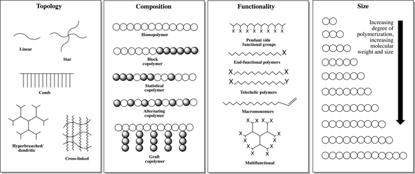
Polymers are ubiquitous in their use spanning a vast range of materials due to their highly tunable physical and chemical properties. They are critical enablers of many modern and emerging technologies today, ranging from structural material used to build modern aircraft, to flexible electronics, and even emulsifiers in personal care products—arguably making them one of the most important classes of material that exist. The properties that govern their specific use are influenced by the architecture or structure,[Reference Gregory and Stenzel1] made up of the following four parameters: topology, composition, functionality, and size (Fig. 1). Fine control of polymer architecture and a deep understanding of its relationship with physiochemical properties is what allows for the innovation of materials with novel properties with important end-applications.[Reference Garcia2–Reference Kumar, McDowall, Chen and Stenzel7]
An illustration of the four fundamental parameters of polymer architecture, namely, topology, composition, functionality, and size that influence the properties of a polymer.

Polymer properties are influenced by either polymer dynamics or chemo-functionality or both. Polymer dynamics are governed by the entanglement and flexibility of the polymer chain, which in turn influence physical properties such as rheology, glass transition temperature, and mechanical properties. Chemo-functionality affords the polymer chains’ chemical response, biologic activity, and electro-chemical activity.
A combination of the two results in interesting morphological and phase characteristics, as well as stimuli-responsive characteristics, which have been thoroughly exploited in drug delivery.[Reference Correa-Baena, Hippalgaonkar, van Duren, Jaffer, Chandrasekhar, Stevanovic, Wadia, Guha and Buonassisi8]
Apart from understanding structure–property relationships, the mechanism, and kinetics of polymerization, the process of polymer synthesis is also a critical area of study of importance when preparing tailored material to fine-tune polymer properties.
For instance, copolymerization compositional relationships between your reaction feed and final product is governed by the Mayo–Lewis equation, which relates the two monomers with their reactivity ratio, a function of their propagation rate constants. The ability to use the equation as an accurate calculator depends on several factors, most important of which is the reactivity ratio. Other factors include the type of polymerization and the conversion. Reactivity ratios are not readily available for all monomer combinations, which have to typically be calculated through extensive and systematically controlled experiments.
State-of-the-art in polymer design
The unique behavior of polymers comes about due to the complexity of the material across multiple length scales. When focusing on a molecular level, these are interactions of a single repeating unit on a polymer to: (1) the unit next to it; (2) the penultimate unit next to it; (3) other units on the polymer chain in the event of the chain coiling on itself, inclusive of the end-group; (4) the solvent or other molecules that are mixed with the polymer; and (5) repeat units of other polymers. The extent of these interactions is often multiplied with increasing polymer size, concentration of the polymer and components, other dissolved compounds in solution and the temperature.
In certain cases, forward empirical, physical, and kinetic models, or mathematical equations governing a particular relationship, provide an excellent predictive tool with high accuracy. Examples of these include the Flory–Fox, Mark–Houwink, Carothers, and Mayo–Lewis equations.
 $$T_{\rm g}\, = \,T_{{\rm g},\infty} -\displaystyle{K \over {M_{\rm n}}}$$
The above Flory–Fox equation describes an empirical forward model, which is commonly used to relate the molecular weight dependence of the glass transition temperature (T g) of polymers. The T g of a polymer is a function of the glass transition temperature of the polymer at infinite molecular weight (T g,∞), the molecular weight of the polymer and a constant (K).
 $$\lsqb \eta \rsqb = KM^a$$
The above Mark–Houwink equation relates the intrinsic viscosity [η] to molecular weight (M) with the coefficients K and a unique for each polymer and architecture. One of the primary uses of this equation is in the determination of molecular weight distribution via size exclusion chromatography using a refractive index detector. Typically, this model generalizes well when calibrating instruments with a dissimilar polymer to the analyte.
 $$\bar{X}_n = \displaystyle{1 \over {1-p}}\quad \bar{X}_n = \displaystyle{{1 + r} \over {1 + r-2rp}}$$
The above equations are part of the Carothers equations that relate the degree of polymerization from fractional monomer conversion for step-growth polymerization. The two equations are meant for linear copolymerization where the two monomer constituents are either equal or unequal in ratio respectively, where the average degree of polymerization, X̄ n is a function of the conversion, p, and the stoichiometric ratio of reactants, r. Derivations of the two equations have also been made to capture the complexity of branched polymers with multifunctional monomers.
 $$F_1 = 1-F_2 = \displaystyle{{r_1f_1^2 + f_1f_2} \over {r_1f_1^2 + 2f_1f_2 + r_2f_2^2}} $$
 $$\displaystyle{{d[M_1]} \over {d[M_2]}} = \displaystyle{{[M_1](r_1[M_1] + [M_2])} \over {[M_2]([M_1] + r_2[M_1])}};\quad r_1 = \displaystyle{{k_{11}} \over {k_{12}}}\quad r_2 = \displaystyle{{k_{22}} \over {k_{21}}}$$
The Mayo–Lewis equation much like the Carothers equations is part of a larger group of equations that govern or are governed by the kinetics polymerization. This equation calculates the distribution of monomers in a two monomer batch copolymerization. The final composition, F 1 is a function of the reactivity ratios (which are in turn a function of the reactivity rate coefficients) and the feed composition of the monomers.
However, beyond this, simple forward models for structure–property relationships are rare. Thus, either molecular dynamics simulations or experimentation have been traditionally employed to map the relationship in this multi-variable parameter space. Bicerano demonstrates how with an increasing amount of available data, efforts have also been made towards the quantitative prediction of polymer properties based on the topological information through their connectivity indices.[Reference Bicerano9]
Stuart et al. highlighted a vast number of experiments where phase behavior of polymers in solution was modulated by external stimuli, which shed light on structure–property relationships, reported in the form of plots and tables.[Reference Stuart, Huck, Genzer, Muller, Ober, Stamm, Sukhorukov, Szleifer, Tsukruk, Urban, Winnik, Zauscher, Luzinov and Minko10] While these carefully conducted experiments have been the starting point for numerous synthetic chemists, the method itself is archaic, having been the only way of dissemination for multiple decades.[Reference Jiang, Jin, Li, Ding and Shi11–Reference Halperin, Kröger and Winnik13] However, this method does not scale, nor does it succinctly capture the multi-variable parameter space of phase properties, as is the case with many other physical properties of polymers. In fact Halperin et al. discuss that after several decades, this area of research is now in its maturity yet we have still not been able to derive a clear, quantitative understanding of not only phase behavior, but also many other structure-property relationships.[Reference Halperin, Kröger and Winnik13]
An expected evolution from the norm was the attempt by Hoogenboom et al., who demonstrated that a quadratic equation was adequate in predicting the temperature responsive phase behavior of a particular copolymer based on its molecular weight and composition.[Reference Hoogenboom, Thijs, Jochems, van Lankvelt, Fijten and Schubert14] While definitely an advance, this technique is limited by its simplicity, restricted to a variable space of three. The approach also makes the assumption that this relationship is quadratic, which may contribute to a poor fit of the data.
In polymerization kinetics, Stockmayer and Flory attempted to solve the Carothers equation for predicting the extent of gelation in a polymerization statistically.[Reference Odian15] A number of assumptions are made to simplify the variable space, including ones that may not necessarily be true such as the absence of intra-polymeric reactions and that the reactivity of all functional groups are the same. The calculations were originally performed by hand and the calculations are iterative in nature. A method such as this could be prone to error, not only due to the assumptions, but also the fact that detailed information and meticulous calculation would be required for accuracy.
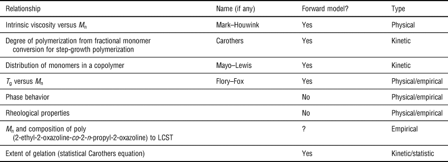
These examples are non-exhaustive, and there are numerous others such as the relationship of rheological properties to architecture, and other polymer interactions. A summary of all the forward model and relationships discussed in this section is provided in Table I.
A non-exhaustive summary of polymer relationships and models commonly studied.

A new approach to polymer design
A key challenge thus is a succinct way to parameterize structure–property relationships. Both the quadratic (or polynomial) and manual statistical methods mentioned above attempt to deal with the multi-parameter space, but often find themselves falling short as the complexities of such a space are often non-trivial and thus require numerous assumptions. This almost always leads to important parameters being overlooked.
A computational data-driven approach to predictive modeling would be able to relate the data in a more rapid and complete manner, and could be a strategy to overcome the aforementioned challenges.[Reference Smith, Isayev and Roitberg16] There are two broad classes of methods, namely statistical models (such as multivariate analysis[Reference Anderson17] and Bayesian inference[Reference Box and Tiao18]) and machine learning models (such as support vector machines,[Reference Cortes and Vapnik19] decision tree learning,[Reference Rokach and Maimon20] and deep neural networks.[Reference LeCun, Bengio and Hinton21]) Statistical models usually perform well on relatively small datasets, but require nontrivial domain information, such as statistical priors and the form of the relationship between inputs to outputs such as a mathematical or forward model. These may not be immediately obvious for some applications, but they severely impact model accuracy and may limit applicability. On the other hand, machine learning models tend to make minimal assumptions and directly learn representations and relationships from data. For sufficiently large datasets, it is often more robust when the underlying mechanisms that links the input and the outputs are unclear, or when the dataset has unknown systematic and random noise corruptions.[Reference Friedman22] Of course, one disadvantage of machine learning-based methods is that, unlike statistical models, besides the final prediction very little can be inferred about the underlying physical process that produced the data. Nevertheless, in many situations when the key goal is producing accurate predictions, machine learning methods are well-suited.
A further advantage of machine learning-based predictive modeling is fast inference speed. Once a model is trained, it can make predictions quickly on previously unseen data. This is especially important in inverse design, where a (global) optimization algorithm is required to minimize some objective that depends on our data-driven model. This involves repeated calls to the fitted predictive model, which must be fast to ensure an extensive search over the desired parameter space. In this sense, simulation-based predictive models will be prohibitively slow and computationally expensive for such an optimization and design process.
Machine learning serves as an enabling tool that allows us to work in a multi-variable parameter space when mapping polymer architecture to a physical property. In the case of cloud points, the traditional technique would be to generate multiple detailed phase plots for systematically varied polymer composition,[Reference Aseyev, Tenhu, Winnik, Müller and Borisov23] an empirical approach similar to examples above. Such curation is often slow, laborious, and could be prone to error with inconsistencies in data quality. In contrast, machine learning is able to map datasets that may not be systematically varied, or consistent in quality, into one unifying algorithm that is agnostic of any assumptions and takes all variables into account.
State-of-the-art for polymer and small molecule design by machine learning
The Aspuru-Guzik team has looked toward incorporating experimental intuition into algorithms capable of predicting a number of key parameters in the synthesis and development of small molecules—the outcome of organic reactions,[Reference Wei, Duvenaud and Aspuru-Guzik24] design of organic light emitting diodes,[Reference Gómez-Bombarelli, Aguilera-Iparraguirre, Hirzel, Duvenaud, Maclaurin, Blood-Forsythe, Chae, Einzinger, Ha, Wu, Markopoulos, Jeon, Kang, Miyazaki, Numata, Kim, Huang, Hong, Baldo, Adams and Aspuru-Guzik25] and energy harvesting materials.[Reference Häse, Kreisbeck and Aspuru-Guzik26,Reference Benjamin, Carlos, Gabriel L. and Alan27] The approach of this team is focused on an inter-disciplinary cohesion of their core-competence in small molecule synthesis and quantum mechanics, along with high-throughput density functional theory (DFT) calculations of molecular descriptors,[Reference Duvenaud, Maclaurin, Aguilera-Iparraguirre, Gomez-Bombarelli, Hirzel, Aspuru-Guzik and Adams28] enabled by the computing power of machine learning methods.[Reference Gómez-Bombarelli, Wei, Duvenaud, Hernández-Lobato, Sánchez-Lengeling, Sheberla, Aguilera-Iparraguirre, Hirzel, Adams and Aspuru-Guzik29] Their powerful data-driven method has shown tremendous promise to not only understand the inherent complex physiochemical properties of an organic molecule, but also how it could be synthesized. While the strategies exhibited in the work might be transferrable to other domains, it seems challenging when facing the complexity of polymers, particularly in structure–property relationships.
The first attempt toward a machine learning approach for the prediction of polymer properties was by the Ramprasad group. The polymer genome initiative utilized machine learning for the accelerated prediction of the dielectric properties of bulk polymers.[Reference Huan, Mannodi-Kanakkithodi, Kim, Sharma, Pilania and Ramprasad30] The approach leverages on a “fingerprinting” methodology,[Reference Mannodi-Kanakkithodi, Pilania, Huan, Lookman and Ramprasad31] whereby DFT calculations for the individual repeat units of the polymer are performed to understand its physical properties, and the polymer properties are derived from a statistical learning algorithm. Their latest strategy leverages at a combination atomic level, quantitative structure–property relationship (QSPR), and morphological descriptors, which is accurate in the prediction of bulk polymer properties calculated by DFT.[Reference Kim, Chandrasekaran, Huan, Das and Ramprasad32] This approach was also accurate in its prediction of experimentally obtained properties such as glass transition temperature (T g), solubility, and density, critical descriptors were simplified, which could render these techniques inaccurate when more robustly tested. An example is that for T g, molecular mass was assumed to be infinite, rather than incorporating the additional descriptors of the Flory–Fox relationship between T g and M n. In a similar approach, Zeng et al. demonstrated that crystallography files may be a sufficient descriptor that provides highly accurate prediction of bandgap and dielectric constant of polymers via crystal graph convolutional neural networks.[Reference Zeng, Kumar, Zeng, Ramasamy, Chandrasekhar and Hippalgaonkar33]
Most of these datasets were generated by high-throughput DFT calculations, with only minimal experimental validation. Wei et al. demonstrated the efficacy of neural networks from simulated data for the inherently more complex scenario of polymer phase behavior in solution.[Reference Wei, Melko and Chen34] Highly accurate demonstrations of machine learning on simulated data may be fallacious since both the latter and the former are computed relationships to their descriptors, leading to cyclic argument, but their efforts clearly show that machine learning could a powerful tool in polymer property prediction. However, none of these teams demonstrate inverse design where input parameters are predicted based on a desired output. The next milestone thus would be a forward predictive machine learning algorithm trained on experimental data, and the experimental validation of the inverse design of this model.
In work recently conducted by our team,[Reference Kumar, Li, Tang, Buonassisi, Gonzalez-Oyarce and Ye35] we demonstrate the use of a combination of machine learning methods to map a design space of composition from four possible monomers and the molecular weight of the polymer to the lower critical solubility temperature (LCST) of poly(2-oxazoline). Predictions from gradient boosting with decision trees had a mean square error of 4°C over a temperature range of 24–90°C (6% error). The fast inference speed of the machine learning algorithm allowed for the inverse design via particle swarm optimization. When cross validated with an ensemble of neural networks, the inverse design was capable of designing 17 unique polymers, including terpolymers, with a mean squared error of 6.1°C. These polymers were designed for four target LCSTs, with constraints such as maximum molecular weight and preferred composition imposed. This is likely to be the first of many research efforts that demonstrate the efficacy machine learning enabled polymer design. The conceptual advance of all the teams mentioned is the progression from the traditionally accepted forms of data representation toward one that is far more robust and intuitive.
The challenges in machine learning augmented polymer design
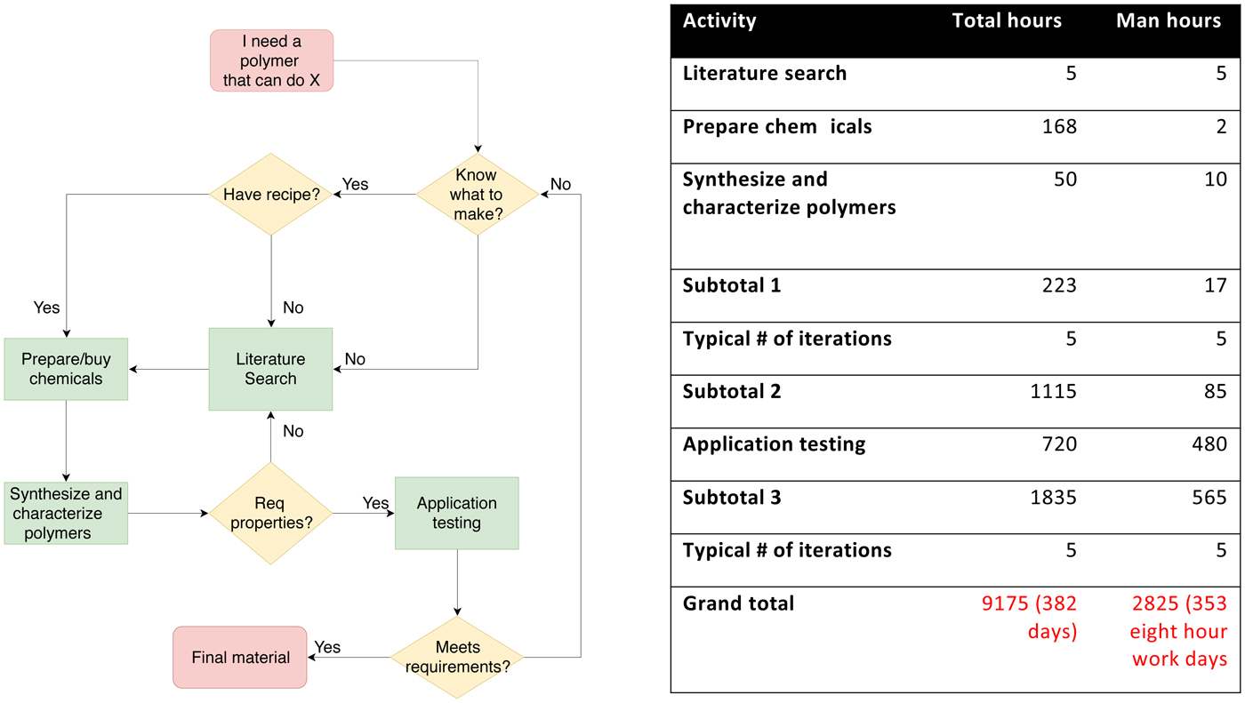
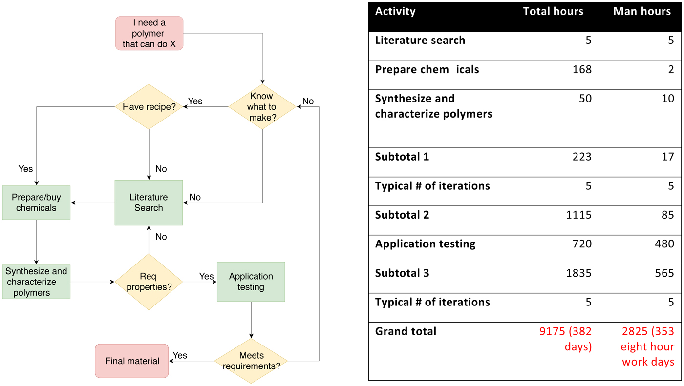
Nevertheless, this approach is not without its challenges, the greatest of which is that the application of data driven techniques to polymer science required large datasets. In the previously mentioned examples, the smallest dataset had 171 unique polymers while the rest were at least a factor of ten greater. While the training datasets could be simulated in a larger and more efficient manner by the methods suggested by the Ramprasad group,[Reference Kim, Chandrasekaran, Huan, Das and Ramprasad32] manual experimentation is typically slower. The flowchart and table in Fig. 2 demonstrate a typical experimentation process from ideation to final product. The length of time it takes to generate one experimental data point can typically be 223 h or about 9 days (subtotal 1), while the time taken to generate one new material could take as much as 353 work days, or about 70 five-day work weeks continuously. The reason for this slow speed is attributed to the limits of the human ability. While the quantity of unique polymers might be low, as is the case in the research of most other materials, the data obtained are often rich in detail. These details comprise of descriptors and attributes—the latter a function of the former. In order to improve the efficacy of machine learning techniques on scarce datasets, two strategies—data curation and data augmentation, should be employed.
(Left) Flowchart of a typical development process of a polymer from ideation to a final material or product; (right) typical timeline of the completion of a new polymer development process.
Data curation is the necessary to mitigate over-complexity over the search space and optimize the training of the forward predictive model. A prime example of the curation of descriptors was demonstrated by Zeng et al.[Reference Zeng, Kumar, Zeng, Ramasamy, Chandrasekhar and Hippalgaonkar33] where they used crystallography data to train a graph convolutional neural network as a predictor for dielectric constant and bandgap of polymers. This was a step forward from the work by the Ramprasad group, which used three sets of descriptors to predict the same properties. Another example is where the shape of the molecular weight distribution was a determining factor in choosing the peak molecular weight rather than the number average molecular weight for thermally responsive polymers.[Reference Kumar, Li, Tang, Buonassisi, Gonzalez-Oyarce and Ye35] Feature importance rankings, which are typical in machine learning algorithms might also assist in determining the best descriptors for the dataset, in a bid to further refine and tune the algorithm.[Reference Luca, Jan, Emre, Runhai, Sergey and Claudia36]
While experimental data are the most important, supplementing these data with those from modeling and simulations could also be valuable in providing a well-rounded dataset. However, modeling the key physical and chemical processes in polymers that directly relate to its physical property by modern molecular simulation techniques such as classical molecular dynamics simulation[Reference Dünweg and Kremer37] or dissipative particle dynamics simulations[Reference Groot and Warren38] come with their own challenges. The length scales for such phase behavior are normally within the range of hundreds of nanometers with timescales within seconds to minutes.[Reference Halperin, Kröger and Winnik13] Molecular simulations are usually capable of dealing with a simulation system composed of millions of atoms to maximum of billion atoms, equivalent to a small cubic box of water with its box length smaller than 1 µm.[Reference Kutzner, Páll, Fechner, Esztermann, de Groot and Grubmüller39] In order to obtain usable data resembling the dynamics of the system within 1 ms of real time for conventional simulation systems as large as that with 1 million atoms equivalent to a cubic box of water molecules with box length around 20 nm, it would require expensive high-performance computers to perform simulations with hundreds and thousands of CPUs continuously for weeks or even months.[Reference Kutzner, Páll, Fechner, Esztermann, de Groot and Grubmüller39] Therefore, while data from simulations cannot be generated rapidly for specific polymer properties such as T g and T c, these data, along with experimental data, could piece together a far more valuable data space than just either alone. On the other hand, promoting accuracy of molecular simulations to reach that is comparable with DFT calculations via machine learning-based potential and/or accelerating molecular simulations through machine learning approaches are on-going efforts in the molecular simulation community.
The solution to accelerate the experimentation process lies in high-throughput experimentation. In a recent review article by Oliver et al.,[Reference Oliver, Zhao, Gormley, Chapman and Boyer40] a number of high-throughput experimentation strategies to generate large polymer libraries via controlled radical polymerization were summarized. The cited examples focus on the enabling capabilities that high-throughput experimentation have on experimenting over a large parameter space when understanding combinatorial polymer synthesis and its kinetics. The ability to generate vast libraries of polymers with precisely controlled variation of precursors and conditions shows how much promise there is from such a tool. There is only one cited example where high-throughput experimentation in both synthesis and application testing of polymer systems, where the efficacy in nucleic acid complexation and delivery were ascertained for core–shell polymer nanoparticles.
Opportunities
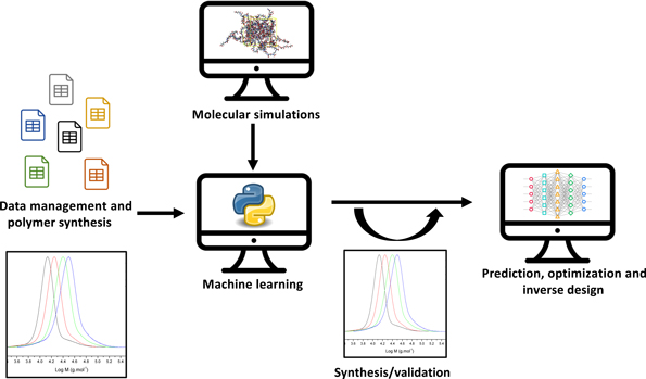
All that we have explored point to three key points that should be the tenets of machine learning augmented polymer design: (1) experimental data are the most important data, and could be generated rapidly by high-throughput experimentation; (2) this should be supplemented by simulated data; and (3) to rationalize this data, proper curation of data should be conducted. Therefore, we propose a framework toward machine learning augmented polymer design, comprising discrete process steps illustrated in Fig. 3.
The proposed framework for machine learning augmented polymer design which incorporates the following steps: data management and polymer synthesis; machine learning; molecular simulations; synthesis/validation; and prediction, optimization and inverse design.
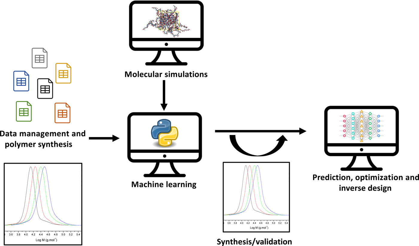
The first and most important step is in data management, where historic and new data should be curated and archived in a manner that adequately captures the detail of the polymer attributes, yet is simple enough and is in a format that lends itself to computation. In this step, datasets can also be augmented by conducting well controlled experiments with diligence paid toward data acquisition.
The second step involves molecular simulations, which is capable of generating data that are not easily accessible by experiments. An example of this is the ability to provide the distribution of monomers in a statistical copolymerization. Yet another would be the physical models such as the QSPR of the repeat unit that could aid in providing a constraint to the machine learning search space.
The third step is machine learning, where the proper selection of the algorithm, along with its tuning, is the primary focus. The improper selection of algorithm or tuning parameters could lead to over-fitting—a common occurrence in relatively small datasets. For a forward predictive model, accuracy of the algorithm is critical. As discussed earlier a short inference time is critical when inverse design is desired. Forward algorithms with slow inference times might be too computationally expensive in such cases.
The final steps involve the experimental validation of the forward model, inverse design, and finally its own experimental validation. When conducted uniformly over the composition, configuration, and attribute space, experimental validation of the forward algorithm has two functions. The first is to verify the accuracy of the machine learning algorithm with a fresh set of “unseen” data. The second is to further train and improve the algorithm. Typically, a well-trained algorithm from the previous step should afford similar accuracy to the original training exercise and this new data serves to lower the total error. This loop train-validation loop should be repeated to increase the predictive accuracies of the forward models to desired levels.
Inverse design is the step where the polymer is designed based on the desired attributes. In many cases, the prediction of descriptors based on desired attributes can have numerous solutions. In order to streamline these, constraints need to be imposed on the search space. These constraints can be made up of experimental experience, domain knowledge, or physical models that can be imposed by simulated data. In addition to these, one or an ensemble of other suitable, but slower predictive algorithms could be used to down-select only the predictions with the highest level of agreement across all algorithms. This would be especially useful in cases where there is extrapolation outside of the original design space. After down-selection, the designs with the highest chance of accuracy should be synthesized to verify the accuracy of the algorithm.
Conclusion and vision
High-throughput experimentation for both synthesis and application testing, combined with a well-designed machine learning algorithm of robust architecture, high performance computing and a scalable data management strategy based on the framework presented above, could pave the way toward an autonomous lab,[Reference Correa-Baena, Hippalgaonkar, van Duren, Jaffer, Chandrasekhar, Stevanovic, Wadia, Guha and Buonassisi8] similar to the success story shown previously for carbon nanotube growth by Nikolaev et al.[Reference Nikolaev, Hooper, Webber, Rao, Decker, Krein, Poleski, Barto and Maruyama41] The combination of all the tools which are now of increasingly easy to access, would provide more value than the sum of its parts and a remarkable advance to the archaic Edisonian research methodology carried out today.
Our vision thus is to enable the translation of the present manual research process into a fully automated system requiring little to no human intervention after the experimental space has been designed. The challenge however, will be the algorithmization of experimental intuition, and the insertion of random error to allow for serendipitous discovery.
Acknowledgments
J.N.K. and Q.L. are supported by the AME Programmatic Fund from the Agency for Science, Technology and Research under Grant No. A1898b0043. The concepts put forward in this paper were developed through discussions with Prof. Tonio Buonassisi, Dr. Kedar Hippalgaonkar, and Dr. Anibal L. Gonzalez-Oyarce.