1 Introduction
Media-based event data—i.e., data comprised from newspaper, television, or web-based accounts—are widely used in research in political science, economics, sociology, and geography. Earl et al. (Reference Earl, Martin, McCarthy and Soule2004) details the centrality of these data in the research on collective action—e.g., racial violence, agrarian protest, social movements—arguing that for such issues there is simply “no other alternative available.” In comparative politics, these data are used in the study of coups, demonstrations, natural disasters, elections, terrorism, and other forms of political violence. Research on intrastate conflict, in particular, frequently uses media-reported data to assess subnational variation in violence and gain greater leverage on the mechanisms which produce conflict (Weidmann Reference Weidmann2016). International Relations research has long used event data to detail the wide array of political interactions between countries, from disputes to diplomacy (Schrodt and Gerner Reference Schrodt and Gerner1994). Media-based measures can be particularly important when political actors wish to conceal their behavior—as frequently occurs, in areas as diverse as human rights violations and Chinese development finance to Africa (Strange et al. Reference Strange, Park, Tierney, Fuchs, Dreher and Ramachandran2013). Studies relying on media-based data will likely to continue to grow, as these data become more abundant and research questions become increasingly granular (Schrodt Reference Schrodt2012).Footnote 1
Despite the broad and frequent use of these data, however, Woolley (Reference Woolley2000, p. 177) notes that “[m]edia sources may not provide good data even though the data are sometimes easily obtained.” In particular, concerns over measurement error are often raised, as news sources do not report all events.Footnote 2 The extent of this underreporting is difficult to assess—as we rarely possess true population rates—yet, some studies have estimated that nearly half of true events go unreported. This incomplete or selective reporting is often attributed to either a lack of opportunity during news gathering (e.g., the distance of a reporter to an event) or willingness during news reporting (e.g., the severity of an event, perceived audience demand, political bias of the media outlet), resulting in the systematic exclusion of particular events from media and resultant data.Footnote 3 Issues that are even further compounded when reporting on any illegal, illicit, or otherwise socially disapproved behavior—from corruption (e.g., vote buying, bribes ) to conflict (e.g., coups, repression)—that are often of interest in social science. Consequently, data from these reports are misclassified—wherein some true events are coded as zeros—and analysis suffers from bias, with inferences which are sensitive to the choice of the source. Despite wide knowledge of these limitations, the threat of reporting bias is often ignored in applied research utilizing event count data. Where solutions have been proposed, researchers are advised to “triangulate” their data—draw from multiple news sources—to reduce the bias introduced from any one source, or to correct for the bias in estimation by modeling the misclassification (Hug and Wisler Reference Hug and Wisler1998; Hug Reference Hug2003, Reference Hug2009).
While either of these approaches is preferable to ignoring possible misclassification outright, we argue that neither is able to fully exploit all of the information commonly possessed by researchers with media-based event data. Namely, no strategy allows researchers to use multiple sources of reporting and misclassification-robust estimation. Briefly summarizing existing approaches, where only one source of (suspected to be incomplete) information is possible—that is, triangulation cannot be accomplished—we agree that researchers should use misclassification-robust methods (Copas Reference Copas1988; Carroll and Pederson Reference Carroll and Pederson1993; Hausman et al. Reference Hausman, Abrevaya and Scott-Morton1998). Where instead multiple sources of information are available, we agree that this should also be leveraged. However, the aggregation of these sources only attenuates, not eliminates, underreporting in the data, meaning additional statistical remedies for misclassification should still be employed. Yet, as none of the current misclassification-robust estimation strategies are derived for this kind of multi-source data-generating process, their application to these data will result in bias or loss of efficiency. Therefore, we propose a misclassification-robust maximum likelihood estimator for multiple sources of data, allowing researchers to estimate the extent of misclassification in each source, and obtain the correct estimates of event of interest. We further generalize our estimator to allow researchers to estimate models where misclassification is dependent upon covariates.
While the focus of our discussion centers largely on media-sourced data, our method is more general than this suggests. Any time a researcher possesses multiple sources of information (e.g., U.S. Department of State vs. United Nations reports) on a qualitative outcome of interest our estimator may be of use.Footnote 4 In the next section we briefly summarize the implications of response measurement error in discrete-outcome models. Next, we introduce our multi-source misclassification estimator. Following that, we outline and present results from Monte Carlo simulations evaluating our estimator against plausible alternatives. Anticipating our findings, we show that neglecting misclassification, by estimating a standard probit, never recovers the true effect estimate when there is differential misclassification, indicating the clear need to adopt corrections such as ours.Footnote 5 We then apply our method to a model of repression using the Social Conflict in Africa Database. Finally, we detail and discuss extensions of our approach to more general applied settings—e.g., scaling the estimator for data with many sources, analyzing nonbinary qualitative outcomes, underreporting in sample selection—before concluding.
2 Measurement Error as Misclassification
Concern over measurement tends to focus predominately on error in predictors rather than error in responses. In part, this is because classical measurement error in the outcome of a linear regression “only” increases the variability of fitted lines without otherwise causing bias to the slope estimates. As discussed in Carroll et al. (Reference Carroll, Ruppert, Stefanski and Crainiceanu2006), this is not the case in discrete-outcome models, where measurement error is misclassification; risking not only a loss of precision but also bias in effects estimates. This can take two forms:
(1) Nondifferential misclassification—when the observed outcome is independent of the covariates conditional upon the actual outcome, that is, the event predictors do not also predict classification—induces severe attenuation bias in parameter estimates.Footnote 6 Whereas, in linear regression there is no such impact.
(2) If instead there is a relationship between the observed response and the model predictors, independent of the true-event risk—i.e., differential misclassification—the bias in the effect estimate can be positive or negative depending on the sign and magnitude of the relevant covariances.
In sum, misclassification in binary-outcome models not only suppresses true relationships—via attenuation or loss of power—but can also induce false positives through inflated effect estimates.Footnote 7
To elaborate more formally, consider the familiar latent-variable representation of the binary-outcome model
 $$\begin{eqnarray}\mathbf{Y}^{\ast }=\unicode[STIX]{x1D6FD}_{0}+\unicode[STIX]{x1D6FD}_{1}^{t}\mathbf{X}+\unicode[STIX]{x1D750},\end{eqnarray}$$
with latent-
 $\mathbf{Y}^{\ast }$
mapping onto the observed, censored outcome
 $\mathbf{Y}_{\mathbf{T}}$
via the standard measurement equation
 $$\begin{eqnarray}\mathbf{Y}_{\mathbf{T}}=\unicode[STIX]{x1D7D9}(\mathbf{Y}^{\ast }\geqslant 0),\end{eqnarray}$$
where
 $\mathbf{Y}_{\mathbf{T}}$
is the true outcome—equal to 1 if an event occurs. This has a probability of response
 $$\begin{eqnarray}\text{pr}(\mathbf{Y}_{\mathbf{T}}=1|\mathbf{X})=F(\unicode[STIX]{x1D6FD}_{0}+\unicode[STIX]{x1D6FD}_{1}^{t}\mathbf{X}).\end{eqnarray}$$
If, however, some set of outcomes in
 $\mathbf{Y}_{\mathbf{T}}=1$
is coded in
 $\mathbf{Y}=0$
, or vice versa, such that
 $$\begin{eqnarray}\text{pr}(\mathbf{Y}=1|\mathbf{Y}_{\mathbf{T}}=0)+\text{pr}(\mathbf{Y}=0|\mathbf{Y}_{\mathbf{T}}=1)\neq 0,\end{eqnarray}$$
there is misclassification. That is, misclassification occurs whenever the outcome vector,
 $\mathbf{Y}$
, used in analysis, erroneously records some true events as zero and/or some nonevents as one.Footnote
8
With nondifferential misclassification, the probability of accurate classification is
 $$\begin{eqnarray}\displaystyle \text{pr}(\mathbf{Y}=1|\mathbf{Y}_{\mathbf{T}}=1,\mathbf{X}) & = & \displaystyle \text{pr}(\mathbf{Y}=1|\mathbf{Y}_{\mathbf{T}}=1)=\unicode[STIX]{x1D70B}_{1},\nonumber\\ \displaystyle \text{pr}(\mathbf{Y}=0|\mathbf{Y}_{\mathbf{T}}=0,\mathbf{X}) & = & \displaystyle \text{pr}(\mathbf{Y}=0|\mathbf{Y}_{\mathbf{T}}=0)=\unicode[STIX]{x1D70B}_{0}.\nonumber\end{eqnarray}$$
This means that the probability for
 $\mathbf{Y}$
in not given by Equation (1), but instead
 $$\begin{eqnarray}\text{pr}(\mathbf{Y}=1|\mathbf{X})=(1-\unicode[STIX]{x1D70B}_{0})+(\unicode[STIX]{x1D70B}_{1}+\unicode[STIX]{x1D70B}_{0}-1)F(\unicode[STIX]{x1D6FD}_{0}+\unicode[STIX]{x1D6FD}_{1}^{t}\mathbf{X}),\end{eqnarray}$$
which equals Equation (1) only if
 $\unicode[STIX]{x1D70B}_{0}=\unicode[STIX]{x1D70B}_{1}=1$
(i.e., no misclassification).
As noted above, failing to account for misclassification results in inconsistent and biased effect estimates (Hausman et al.
Reference Hausman, Abrevaya and Scott-Morton1998). Therefore, many strategies to address misclassification has received considerable attention elsewhere (Abrevaya and Hausman Reference Abrevaya and Hausman1999; Copas Reference Copas1988; Carroll and Pederson Reference Carroll and Pederson1993; Hausman et al.
Reference Hausman, Abrevaya and Scott-Morton1998). Two problems persist with these existing remedies. First, many of these, including those enjoying the widest use currently in political science (Hausman et al.
Reference Hausman, Abrevaya and Scott-Morton1998; Hug Reference Hug2009), simply maximize some version of the log-likelihood implied by Equation (2). As noted by Carroll et al. (Reference Carroll, Ruppert, Stefanski and Crainiceanu2006, p. 347), with these estimators “classification probabilities are only very weakly identified…parameters may be identified theoretically but not in any practical sense.” As such, when and where possible, we will want to supply additional information to inform the misclassification probabilities over what we observe simply in
 $\mathbf{Y}$
.
Second, none of these approaches is derived explicitly for the type of situation which motivates our project, that is, several sources of misclassified data. The Hausman et al. (Reference Hausman, Abrevaya and Scott-Morton1998) estimator, for example, is developed for a single misclassified binary outcome, not aggregate data from several sources erroneously treated as if it were a single binary outcome. As a result, the misapplication of this estimator to these data mismodels a fundamental feature of the data-generating process, resulting in a loss of efficiency or bias. In short, these estimators are designed to handle a different experimental condition from the one represented by the data considered heretofore. Therefore, we provide an alternative strategy in the next section.
3 A Multi-source Solution
As discussed in the introduction, misclassification is likely to occur with media-based event data, where primary- or secondary-source reports fail to include the occurrence of an actual event. To introduce our method, consider two news outlets, 1 and 2, providing reports,
 $\mathbf{Y}_{\mathbf{1}}$
and
 $\mathbf{Y}_{\mathbf{2}}$
, on the event of interest
 $\mathbf{Y}_{\mathbf{T}}$
.Footnote
9
Ultimately, we are interested in
 $$\begin{eqnarray}\text{pr}(\mathbf{Y}_{\mathbf{T}}=1|\mathbf{X}),\end{eqnarray}$$
where
 $\mathbf{X}$
is a matrix of predictors of the event. However, we possess two incomplete reports
 $\mathbf{Y}_{\mathbf{1}}\neq \mathbf{Y}_{\mathbf{T}}$
and
 $\mathbf{Y}_{\mathbf{2}}\neq \mathbf{Y}_{\mathbf{T}}$
, explained by:
 $$\begin{eqnarray}\displaystyle & & \displaystyle \text{pr}(\mathbf{Y}_{\mathbf{1}}=1|\mathbf{X},\mathbf{Z}_{\mathbf{1}})\nonumber\\ \displaystyle & & \displaystyle \text{pr}(\mathbf{Y}_{\mathbf{2}}=1|\mathbf{X},\mathbf{Z}_{\mathbf{2}}),\nonumber\end{eqnarray}$$
where
 $\mathbf{Z}_{\mathbf{1}}$
and
 $\mathbf{Z}_{\mathbf{2}}$
are predictors of the (mis-)reporting of an event (e.g., distance to reporting office) by that source, which are otherwise unrelated to
 $\mathbf{Y}_{\mathbf{T}}$
. Following convention in the applied literature, we aggregate these sources to reduce the individual missingness by
 $$\begin{eqnarray}\mathbf{Y}_{\mathbf{s}\mathbf{u}\mathbf{m}}=\unicode[STIX]{x1D7D9}(\mathbf{Y}_{\mathbf{1}}+\mathbf{Y}_{\mathbf{2}}\geqslant 1).\end{eqnarray}$$
If
 $\mathbf{Y}_{\mathbf{s}\mathbf{u}\mathbf{m}}=\mathbf{Y}_{\mathbf{T}}$
, the data are complete and we find that
 $$\begin{eqnarray}\text{pr}(\mathbf{Y}_{\mathbf{T}}=1|\mathbf{X},\mathbf{Z}_{\mathbf{1}},\mathbf{Z}_{\mathbf{2}})=\text{pr}(\mathbf{Y}_{\mathbf{T}}=1|\mathbf{X})=F(\unicode[STIX]{x1D6FD}^{t}\mathbf{X}),\end{eqnarray}$$
where
 $F(\cdot )$
is specified up to the parameter
 $\unicode[STIX]{x1D6FD}$
. However, where
 $\mathbf{Y}_{\mathbf{s}\mathbf{u}\mathbf{m}}\neq \mathbf{Y}_{\mathbf{T}}$
, we are unable to simplify as in (3). This means that when observed outcomes are misclassified, fitting Equation (3) will result in biased estimates of
 $\mathbf{X}$
on
 $\mathbf{Y}_{\mathbf{T}}$
.
Therefore, we construct an estimator around
Assumption 1. We make the following assumptions: (a)
 $\mathbf{Y}_{\mathbf{1}}$
and
 $\mathbf{Y}_{\mathbf{2}}$
are independent given
 $(\mathbf{Y}_{\mathbf{T}},\mathbf{X},\mathbf{Z}_{\mathbf{1}},\mathbf{Z}_{\mathbf{2}})$
. (b)
 $\mathbf{Y}_{\mathbf{s}\mathbf{u}\mathbf{m}}=1$
implies
 $\mathbf{Y}_{\mathbf{T}}=1$
with probability 1. (c)
 $\mathbf{Y}_{\mathbf{T}}=0$
implies that
 $\mathbf{Y}_{\mathbf{s}\mathbf{u}\mathbf{m}}=0=\mathbf{Y}_{\mathbf{1}}=\mathbf{Y}_{\mathbf{2}}$
with probability 1.
Less formally, Assumption 1(a) states that the sources of reporting data are conditionally independent of one another. Assumption 1(b) and Assumption 1(c) jointly indicate that misclassification in this context is exclusively underreporting.
If we treat
 $\mathbf{Y}_{\mathbf{s}\mathbf{u}\mathbf{m}}$
as the response variable, the problem is related to one studied by Copas (Reference Copas1988), Carroll and Pederson (Reference Carroll and Pederson1993), and Hausman et al. (Reference Hausman, Abrevaya and Scott-Morton1998). The misclassification probabilities are
 $$\begin{eqnarray}\displaystyle & & \displaystyle \text{pr}(\mathbf{Y}_{\mathbf{s}\mathbf{u}\mathbf{m}}=0|\mathbf{Y}_{\mathbf{T}}=1,\mathbf{X},\mathbf{Z}_{\mathbf{1}},\mathbf{Z}_{\mathbf{2}})=\unicode[STIX]{x1D6FE}(\mathbf{X},\mathbf{Z}_{\mathbf{1}},\mathbf{Z}_{\mathbf{2}}),\end{eqnarray}$$
 $$\begin{eqnarray}\displaystyle & & \displaystyle \text{pr}(\mathbf{Y}_{\mathbf{s}\mathbf{u}\mathbf{m}}=1|\mathbf{Y}_{\mathbf{T}}=0,\mathbf{X},\mathbf{Z}_{\mathbf{1}},\mathbf{Z}_{\mathbf{2}})=0,\end{eqnarray}$$
where (5) followed from Assumption 1(b). In Hausman et al. (Reference Hausman, Abrevaya and Scott-Morton1998) these misclassification probabilities do not depend of the covariates, and are instead simply an unknown constant to be estimated.Footnote 10 Therefore, we generalize Hausman et al. (Reference Hausman, Abrevaya and Scott-Morton1998)’s estimator to allow for misclassification probabilities that are dependent upon the covariates (as shown in Online Appendix A)
 $$\begin{eqnarray}\displaystyle & & \displaystyle \text{pr}(\mathbf{Y}_{\mathbf{s}\mathbf{u}\mathbf{m}}=0|\mathbf{X},\mathbf{Z}_{\mathbf{1}},\mathbf{Z}_{\mathbf{2}})=\{1-\unicode[STIX]{x1D6FE}(\mathbf{X},\mathbf{Z}_{\mathbf{1}},\mathbf{Z}_{\mathbf{2}})\}\{1-F(\mathbf{X},\unicode[STIX]{x1D6FD})\}+\unicode[STIX]{x1D6FE}(\mathbf{X},\mathbf{Z}_{\mathbf{1}},\mathbf{Z}_{\mathbf{2}});\end{eqnarray}$$
 $$\begin{eqnarray}\displaystyle & & \displaystyle \text{pr}(\mathbf{Y}_{\mathbf{s}\mathbf{u}\mathbf{m}}=1|\mathbf{X},\mathbf{Z}_{\mathbf{1}},\mathbf{Z}_{\mathbf{2}})=\{1-\unicode[STIX]{x1D6FE}(\mathbf{X},\mathbf{Z}_{\mathbf{1}},\mathbf{Z}_{\mathbf{2}})\}F(\mathbf{X},\unicode[STIX]{x1D6FD}).\end{eqnarray}$$
In principle, since the form of
 $F(\cdot )$
is assumed known, then
 $\unicode[STIX]{x1D6FE}(\mathbf{X},\mathbf{Z}_{\mathbf{1}},\mathbf{Z}_{\mathbf{2}})$
is identified nonparametrically. If one assumes a parametric form for
 $\unicode[STIX]{x1D6FE}(\cdot )$
, then maximum likelihood can be employed.
However, the data are not
 $(\mathbf{Y}_{\mathbf{s}\mathbf{u}\mathbf{m}},\mathbf{X},\mathbf{Z}_{\mathbf{1}},\mathbf{Z}_{\mathbf{2}})$
, but
 $(\mathbf{Y}_{\mathbf{1}},\mathbf{Y}_{\mathbf{2}},\mathbf{X},\mathbf{Z}_{\mathbf{1}},\mathbf{Z}_{\mathbf{2}})$
, that is, we have multiple sources of data. As such, there may be different misclassification rates, which is the fundamental difference between our estimator and existing approaches. Rather than neglect this information, thereby failing to use all of the data, we define
 $$\begin{eqnarray}\displaystyle \unicode[STIX]{x1D6FC}_{1}(\mathbf{X},\mathbf{Z}_{\mathbf{1}}) & = & \displaystyle \text{pr}(\mathbf{Y}_{\mathbf{1}}=0|\mathbf{Y}_{\mathbf{T}}=1,\mathbf{X},\mathbf{Z}_{\mathbf{1}});\end{eqnarray}$$
 $$\begin{eqnarray}\displaystyle \unicode[STIX]{x1D6FC}_{2}(\mathbf{X},\mathbf{Z}_{\mathbf{2}}) & = & \displaystyle \text{pr}(\mathbf{Y}_{\mathbf{2}}=0|\mathbf{Y}_{\mathbf{T}}=1,\mathbf{X},\mathbf{Z}_{\mathbf{2}}).\end{eqnarray}$$
Here by Assumption 1(b) we have that
 $\text{pr}(\mathbf{Y}_{\mathbf{1}}=1|\mathbf{Y}_{\mathbf{T}}=0,\mathbf{X},\mathbf{Z}_{\mathbf{1}})=\text{pr}(\mathbf{Y}_{\mathbf{2}}=1|\mathbf{Y}_{\mathbf{T}}=0,\mathbf{X},\mathbf{Z}_{\mathbf{2}})=0$
. Then under Assumption 1(a), it is easy to see that
 $$\begin{eqnarray}\unicode[STIX]{x1D6FE}(\mathbf{X},\mathbf{Z}_{\mathbf{1}},\mathbf{Z}_{\mathbf{2}})=\unicode[STIX]{x1D6FC}_{1}(\mathbf{X},\mathbf{Z}_{\mathbf{1}})\unicode[STIX]{x1D6FC}_{2}(\mathbf{X},\mathbf{Z}_{\mathbf{2}}).\end{eqnarray}$$
Indeed, in Online Appendix A, we show the following result.
Lemma 1. Under Assumption 1 ,
 $$\begin{eqnarray}\displaystyle \text{pr}(\mathbf{Y}_{\mathbf{1}}=0,\mathbf{Y}_{\mathbf{2}}=0|\mathbf{X},\mathbf{Z}_{\mathbf{1}},\mathbf{Z}_{\mathbf{2}}) & = & \displaystyle 1-F(\mathbf{X},\unicode[STIX]{x1D6FD})+\unicode[STIX]{x1D6FC}_{1}(\mathbf{X},\mathbf{Z}_{\mathbf{1}})\unicode[STIX]{x1D6FC}_{2}(\mathbf{X},\mathbf{Z}_{\mathbf{2}})F(\mathbf{X},\unicode[STIX]{x1D6FD});\nonumber\\ \displaystyle \text{pr}(\mathbf{Y}_{\mathbf{1}}=0,\mathbf{Y}_{\mathbf{2}}=1|\mathbf{X},\mathbf{Z}_{\mathbf{1}},\mathbf{Z}_{\mathbf{2}}) & = & \displaystyle \unicode[STIX]{x1D6FC}_{1}(\mathbf{X},\mathbf{Z}_{\mathbf{1}})\{1-\unicode[STIX]{x1D6FC}_{2}(\mathbf{X},\mathbf{Z}_{\mathbf{2}})\}F(\mathbf{X},\unicode[STIX]{x1D6FD});\nonumber\\ \displaystyle \text{pr}(\mathbf{Y}_{\mathbf{1}}=1,\mathbf{Y}_{\mathbf{2}}=0|\mathbf{X},\mathbf{Z}_{\mathbf{1}},\mathbf{Z}_{\mathbf{2}}) & = & \displaystyle \{1-\unicode[STIX]{x1D6FC}_{1}(\mathbf{X},\mathbf{Z}_{\mathbf{1}})\}\unicode[STIX]{x1D6FC}_{2}(\mathbf{X},\mathbf{Z}_{\mathbf{2}})F(\mathbf{X},\unicode[STIX]{x1D6FD});\nonumber\\ \displaystyle \text{pr}(\mathbf{Y}_{\mathbf{1}}=1,\mathbf{Y}_{\mathbf{2}}=1|\mathbf{X},\mathbf{Z}_{\mathbf{1}},\mathbf{Z}_{\mathbf{2}}) & = & \displaystyle \{1-\unicode[STIX]{x1D6FC}_{1}(\mathbf{X},\mathbf{Z}_{\mathbf{1}})\}\{1-\unicode[STIX]{x1D6FC}_{2}(\mathbf{X},\mathbf{Z}_{\mathbf{2}})\}F(\mathbf{X},\unicode[STIX]{x1D6FD}).\nonumber\end{eqnarray}$$
This implies the likelihood function
 $$\begin{eqnarray}\displaystyle L(\unicode[STIX]{x1D6FD},\unicode[STIX]{x1D702}_{1},\unicode[STIX]{x1D702}_{2}) & = & \displaystyle \prod [1-F(\mathbf{X},\unicode[STIX]{x1D6FD})+\unicode[STIX]{x1D6FC}_{1}(\mathbf{X},\mathbf{Z}_{\mathbf{1}},\unicode[STIX]{x1D702}_{1})\unicode[STIX]{x1D6FC}_{2}(\mathbf{X},\mathbf{Z}_{\mathbf{2}},\unicode[STIX]{x1D702}_{2})F(\mathbf{X},\unicode[STIX]{x1D6FD})]^{\mathbf{Y}_{\mathbf{1}}\mathbf{Y}_{\mathbf{2}}}\nonumber\\ \displaystyle & & \displaystyle \times \,[\unicode[STIX]{x1D6FC}_{1}(\mathbf{X},\mathbf{Z}_{\mathbf{1}},\unicode[STIX]{x1D702}_{1})\{1-\unicode[STIX]{x1D6FC}_{2}(\mathbf{X},\mathbf{Z}_{\mathbf{2}},\unicode[STIX]{x1D702}_{2})\}F(\mathbf{X},\unicode[STIX]{x1D6FD})]^{(1-\mathbf{Y}_{\mathbf{1}})\mathbf{Y}_{\mathbf{2}}}\nonumber\\ \displaystyle & & \displaystyle \times \,[\{1-\unicode[STIX]{x1D6FC}_{1}(\mathbf{X},\mathbf{Z}_{\mathbf{1}},\unicode[STIX]{x1D702}_{1})\}\unicode[STIX]{x1D6FC}_{2}(\mathbf{X},\mathbf{Z}_{\mathbf{2}},\unicode[STIX]{x1D702}_{2})F(\mathbf{X},\unicode[STIX]{x1D6FD})]^{\mathbf{Y}_{\mathbf{1}}(1-\mathbf{Y}_{\mathbf{2}})}\nonumber\\ \displaystyle & & \displaystyle \times \,[\{1-\unicode[STIX]{x1D6FC}_{1}(\mathbf{X},\mathbf{Z}_{\mathbf{1}},\unicode[STIX]{x1D702}_{1})\}\{1-\unicode[STIX]{x1D6FC}_{2}(\mathbf{X},\mathbf{Z}_{\mathbf{2}},\unicode[STIX]{x1D702}_{2})\}F(\mathbf{X},\unicode[STIX]{x1D6FD})]^{(1-\mathbf{Y}_{\mathbf{1}})(1-\mathbf{Y}_{\mathbf{2}})}.\nonumber\end{eqnarray}$$
Under our assumptions, this allows us to estimate parameters for the risk-model and misclassification probabilities. This improves over current estimators which either force researchers to erroneously assume that there is no misclassification in the data, that the data originates from one source, or both. Furthermore, our estimator utilizes more data-based information to achieve identification, resulting in sounder estimates of the misclassification and, in turn, event probabilities.Footnote 11
In sum, our estimator allows researchers using event-based data to accurately test theories on both the event of interest and (mis-)reporting of these events.Footnote 12
4 Simulations
Our simulation study is designed to evaluate the performance of estimators under outcome misclassification. We consider the following five methods:
(1) Naïve Probit: fits a probit model to
 $Y_{\text{sum}}$
with event probability
$\text{pr}(Y_{\text{sum}}=1|X)=\unicode[STIX]{x1D6F7}(\unicode[STIX]{x1D6FD}_{0}+\unicode[STIX]{x1D6FD}_{1}X)$
.
(2) Hausman, Constant Probabilities: the approach outlined in Hausman et al. (Reference Hausman, Abrevaya and Scott-Morton1998)—assuming constant misclassification probabilities and exploiting our Assumption 1(b)Footnote 13 —which fits
$\text{pr}(Y_{\text{sum}}=1|X)=\{1-\unicode[STIX]{x1D70B}_{1}\}\unicode[STIX]{x1D6F7}(\unicode[STIX]{x1D6FD}_{0}+\unicode[STIX]{x1D6FD}_{1}X)$
.(3) Hausman with Covariates: our generalization of Hausman et al. (Reference Hausman, Abrevaya and Scott-Morton1998) allowing for nonconstant misclassification probabilities
$\text{pr}(Y_{\text{sum}}=0|Y_{T}=1,X,Z_{1},Z_{2})=\unicode[STIX]{x1D6FE}(X,Z_{1},Z_{2})=\unicode[STIX]{x1D6F7}(\unicode[STIX]{x1D702}_{00}+\unicode[STIX]{x1D702}_{01}X+\unicode[STIX]{x1D702}_{02}Z_{1}+\unicode[STIX]{x1D702}_{03}Z_{2})$
, giving event probabilities
$\text{pr}(Y_{\text{sum}}=1|X,Z_{1},Z_{2})=\{1-\unicode[STIX]{x1D6FE}(X,Z_{1},Z_{2})\}\unicode[STIX]{x1D6F7}(\unicode[STIX]{x1D6FD}_{0}+\unicode[STIX]{x1D6FD}_{1}X)$
.(4) Multi-source, Constant Probabilities: our multi-source method detailed in Section 3, but restricted to use constant probabilities
$\unicode[STIX]{x1D6FC}_{1}(X,Z_{1})=\unicode[STIX]{x1D6F7}(\unicode[STIX]{x1D702}_{10})$
and
$\unicode[STIX]{x1D6FC}_{2}(X,Z_{2})=\unicode[STIX]{x1D6F7}(\unicode[STIX]{x1D702}_{20})$
.(5) Multi-source with Covariates: our general multi-source method detailed in Section 3 with
$\unicode[STIX]{x1D6FC}_{1}(X,Z_{1})=\unicode[STIX]{x1D6F7}(\unicode[STIX]{x1D702}_{10}+\unicode[STIX]{x1D702}_{11}X+\unicode[STIX]{x1D702}_{12}Z_{1})$
and
$\unicode[STIX]{x1D6FC}_{2}(X,Z_{2})=\unicode[STIX]{x1D6F7}(\unicode[STIX]{x1D702}_{20}+\unicode[STIX]{x1D702}_{21}X+\unicode[STIX]{x1D702}_{22}Z_{2})$
.


4.1 Simulation design
The data-generating process for the simulations is the following:
∙ Step I. Take
$n$
draws of
$X,Z_{1}$
and
$Z_{2}$
from a
$N(0,1)$
distribution.∙ Step II. Generate
$Y_{T}$
from a Bernoulli distribution with success probability
$F(X_{i},\unicode[STIX]{x1D6FD})=\unicode[STIX]{x1D6F7}(\unicode[STIX]{x1D6FD}_{0}+X_{i}\unicode[STIX]{x1D6FD}_{1})$
,
$i=1,\ldots ,n$
, where
$\unicode[STIX]{x1D6F7}$
denotes the CDF of the standard normal distribution.∙ Step III. Generate misclassification probabilities using
then generate$$\begin{eqnarray}\displaystyle \unicode[STIX]{x1D6FC}_{1}(X_{i},Z_{i,1}) & = & \displaystyle \unicode[STIX]{x1D6F7}(\unicode[STIX]{x1D702}_{10}+\unicode[STIX]{x1D702}_{11}X_{i}+\unicode[STIX]{x1D702}_{12}Z_{i,1}),\quad \text{and}\nonumber\\ \displaystyle \unicode[STIX]{x1D6FC}_{2}(X_{i},Z_{i,2}) & = & \displaystyle \unicode[STIX]{x1D6F7}(\unicode[STIX]{x1D702}_{20}+\unicode[STIX]{x1D702}_{21}X_{i}+\unicode[STIX]{x1D702}_{22}Z_{i,2}),\nonumber\end{eqnarray}$$
$Y_{i,1}$
and
$Y_{i,2}$
$$\begin{eqnarray}Y_{i,1}=Y_{i,T}(1-B(\unicode[STIX]{x1D6FC}_{1}))\quad \text{and}\quad Y_{i,2}=Y_{i,T}(1-B(\unicode[STIX]{x1D6FC}_{2})).\end{eqnarray}$$
∙ Step IV. Given
$Y_{1}$
and
$Y_{2}$
, generate
$Y_{\text{sum}}$
using
$Y_{\text{sum}}=\unicode[STIX]{x1D7D9}(Y_{i,1}+Y_{i,2}\geqslant 1)$
.


Across all experiments, we generate
 $N=1000$
data sets (i.e., trials), each with sample size
 $n=1000$
. Our experimental data-generation process nests all the methods detailed above, with different assignments to the
 $\unicode[STIX]{x1D702}$
’s producing each of these as the true model. As such, we are mainly interested in the effect of varying those parameters, so we fix
 $\unicode[STIX]{x1D6FD}_{0}=-1$
and
 $\unicode[STIX]{x1D6FD}_{1}=1$
in all experiments (producing
 $\text{pr}(Y_{\text{sum}}=1)\approx 0.30$
).
We investigate the effect of misclassification under two broad sets of experimental conditions produced from different specifications in Step III:
(1) Nondifferential misclassification—the misclassification errors
$\unicode[STIX]{x1D6FC}_{1}$
and
$\unicode[STIX]{x1D6FC}_{2}$
do not depend on the covariates and are constant (i.e.,
$\unicode[STIX]{x1D702}_{10}>0$
,
$\unicode[STIX]{x1D702}_{20}>0$
, and
$\unicode[STIX]{x1D702}_{11}=\unicode[STIX]{x1D702}_{12}=\unicode[STIX]{x1D702}_{21}=\unicode[STIX]{x1D702}_{22}=0$
).Footnote
14
(2) Differential misclassification—the misclassification errors
$\unicode[STIX]{x1D6FC}_{1}$
and
$\unicode[STIX]{x1D6FC}_{2}$
depend on the event covariates (i.e.,
$\unicode[STIX]{x1D702}_{11}>0$
and/or
$\unicode[STIX]{x1D702}_{21}>0$
).


In the next section we provide detailed results from two experiments under these conditions. In Experiment 1 we set
 $\unicode[STIX]{x1D6FC}_{1}=0.35$
and
 $\unicode[STIX]{x1D6FC}_{2}=0.2$
,Footnote
15
drawing on previous studies which have evaluated the extent of misclassification in data of these types, we consider this a moderate level of misclassification which is likely to be observed by researchers. In Experiment 2, we set
 $(\unicode[STIX]{x1D702}_{10},\unicode[STIX]{x1D702}_{11},\unicode[STIX]{x1D702}_{12},\unicode[STIX]{x1D702}_{20},\unicode[STIX]{x1D702}_{21},\unicode[STIX]{x1D702}_{22})=(-0.7,1,1,-1.4,1,1)$
, so that
 $E\{\unicode[STIX]{x1D6FC}_{1}(X,Z_{1})\}\approx 0.35$
and
 $E\{\unicode[STIX]{x1D6FC}_{2}(X,Z_{2})\}\approx 0.2$
. This allows us to evaluate distinct effects of nondifferential and differential error under roughly the same rate of misclassification.Footnote
16
4.2 Results
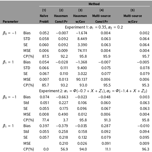
The results of the simulation study are presented in Table 1, with the bias, standard deviation (STD), estimated standard error (SE), and mean-squared error (MSE), and 95% coverage probability (CP) reported.Footnote 17 The top half, Experiment 1, presents the results of our constant, nondifferential error simulations. We see that, as expected, our Multi-source methods (Models 4 & 5) outperform the other methods in MSE terms. Furthermore, the CPs—the proportion of simulations in which the parameter is contained in the interval estimate—for both closely reflect the nominal 95% confidence levels. The alternative estimators, on the other hand, perform noticeably worse. The Hausman with Covariates (Model 3), is obviously flawed when the misclassification probabilities in the DGP are fixed, with estimates varying wildly from simulation to simulation. The Naïve Probit and Hausman Constant estimators perform better than this, but still underperform our proposed estimators. Naïve Probit (Model 1) is only slightly worse in MSE terms, however, the bias and resultant anti-conservative CPs are troubling, while the Hausman-type estimator (Model 2) is nearly two-times worse than our estimators in MSE.
While our estimators do perform well, we do not want to overstate the extent of the gains. In general, the conventional estimation strategies seem to do fairly well if the misclassification rates are truly nondifferential. However, this rarely happens in practice as underreporting is usually systemic, that is, there is a reason why some observations are misclassified and not others (Schrodt Reference Schrodt2012).Footnote
18
Experiment II, the lower half of Table 1, provides the results from simulations under these conditions. We observe a substantial degradation in the performance of the conventional strategies. The Naïve Probit and Hausman Constant estimators have substantial bias in the slope estimates, with MSE orders of magnitude larger than our preferred methods. Moreover, the Naïve Probit estimator never (!) recovers the true sample statistic in any of the simulations (
 $\text{CP}=0.0$
). As this is the dominant empirical strategy used in political science this is clearly a problem.Footnote
19
We see expected gains in the Hausman with Covariates (Model 3) and degradation in Multi-source Constant, reflecting the accuracy with which they capture the true data-generating process. Our Multi-source with Covariates method clearly dominates, with the lowest MSE and most accurate CPs. More importantly, perhaps, is that our Multi-source with Covariates method is robust to either type of misclassification—i.e., differential or nondifferential—as it is nearly dominant in both sets of simulations. Thus, researchers can employ this method when they do not have strong ex ante beliefs over the cause of misclassification in their data and be confident in the results obtained.
Simulation study results.

Note: Included in the table is the average bias of the estimator (Bias), the standard deviation of the estimates across the simulations (STD), the mean estimated standard error (SE), the mean-squared error (MSE), and the coverage probabilities (CPs) of a nominal 95% confidence interval. The estimation methods and experimental conditions are detailed in Section 4.
Parameter estimates are often not directly the quantity of interest. Instead, researchers are interested in some transformation of the parameter, such as the marginal effect, which is not equal to the reported coefficient in all but the linear-additive model. As such, we calculate the marginal effect of
 $X$
for each of the estimators as
 $$\begin{eqnarray}\unicode[STIX]{x2202}Y/\unicode[STIX]{x2202}X=\unicode[STIX]{x1D6F7}\{\hat{\unicode[STIX]{x1D6FD}_{0}}+\hat{\unicode[STIX]{x1D6FD}_{1}}(\unicode[STIX]{x1D707}_{x}+\unicode[STIX]{x1D70E}_{x})\}-\unicode[STIX]{x1D6F7}\{\hat{\unicode[STIX]{x1D6FD}_{0}}+\hat{\unicode[STIX]{x1D6FD}_{1}}\unicode[STIX]{x1D707}_{x}\}.\end{eqnarray}$$
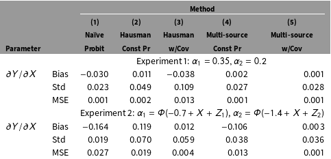
The results of both experiments are given in Table 2. For Experiment 1, we see that as in parameter estimation, all estimators perform quite well in terms of MSE. Naïve Probit has the downward bias we would expect from attenuation in nondifferential misclassification, yet the results from all estimators are fairly encouraging. Experiment II is quite different, here we see substantial bias in each of the estimators that fails to model the misclassification probabilities as a function of covariates. Interestingly, we see a large attenuating bias in Naïve Probit and a large inflationary bias in Hausman Constant, suggesting that rather than solve the problem the Hausman-type estimator simply introduces a new one. As before, we see that our preferred method, Multi-source with Covariates, provides accurate marginal effect estimates under other experimental condition.
Marginal effects in simulation studies.

Note: Included in the table is the average bias of the estimator (Bias), the standard deviation of the estimates across the simulations (STD), and the mean-squared error (MSE). The estimation methods and experimental conditions are detailed in Section 4.
While our estimator performs well under either type of misclassification, two additional issues may be of concern with real data. First, researchers will often not have complete models of misclassification, as such it will be important to know the effect of omitted variables in the misclassification submodels. Second, often sources will not perfectly reflect Assumption 1(a)— i.e., local independence across sources—which was part of the derivation of our estimator above, as such it will be important to know the small-sample implications of violations of this condition.Footnote 20 We explore both concerns in an additional series of simulations where we include additional, correlated unobservables in the generation of the misclassification probabilities:
 $$\begin{eqnarray}\displaystyle \unicode[STIX]{x1D6FC}(X_{i},Z_{i,1}) & = & \displaystyle \unicode[STIX]{x1D6F7}(\unicode[STIX]{x1D702}_{10}+\unicode[STIX]{x1D702}_{11}X_{i}+\unicode[STIX]{x1D702}_{12}Z_{i,1}+u_{1}),\nonumber\\ \displaystyle \unicode[STIX]{x1D6FC}(X_{i},Z_{i,2}) & = & \displaystyle \unicode[STIX]{x1D6F7}(\unicode[STIX]{x1D702}_{20}+\unicode[STIX]{x1D702}_{21}X_{i}+\unicode[STIX]{x1D702}_{22}Z_{i,2}+u_{2}),\nonumber\end{eqnarray}$$
where
 $(u_{1},u_{2})^{\text{T}}=\text{Normal}(0,\unicode[STIX]{x1D6F4})$
, where
 $\unicode[STIX]{x1D6F4}$
is the covariance matrix of a bivariate standard normal random variable with variance
 $=1$
and correlation
 $\unicode[STIX]{x1D70C}$
, with changes to
 $\unicode[STIX]{x1D70C}$
varying the extent of the correlation across the sources. We run 51 additional simulations for Experiment 2 with this modification—evaluating correlations from
 $\unicode[STIX]{x1D70C}=-0.5$
to
 $\unicode[STIX]{x1D70C}=0.5$
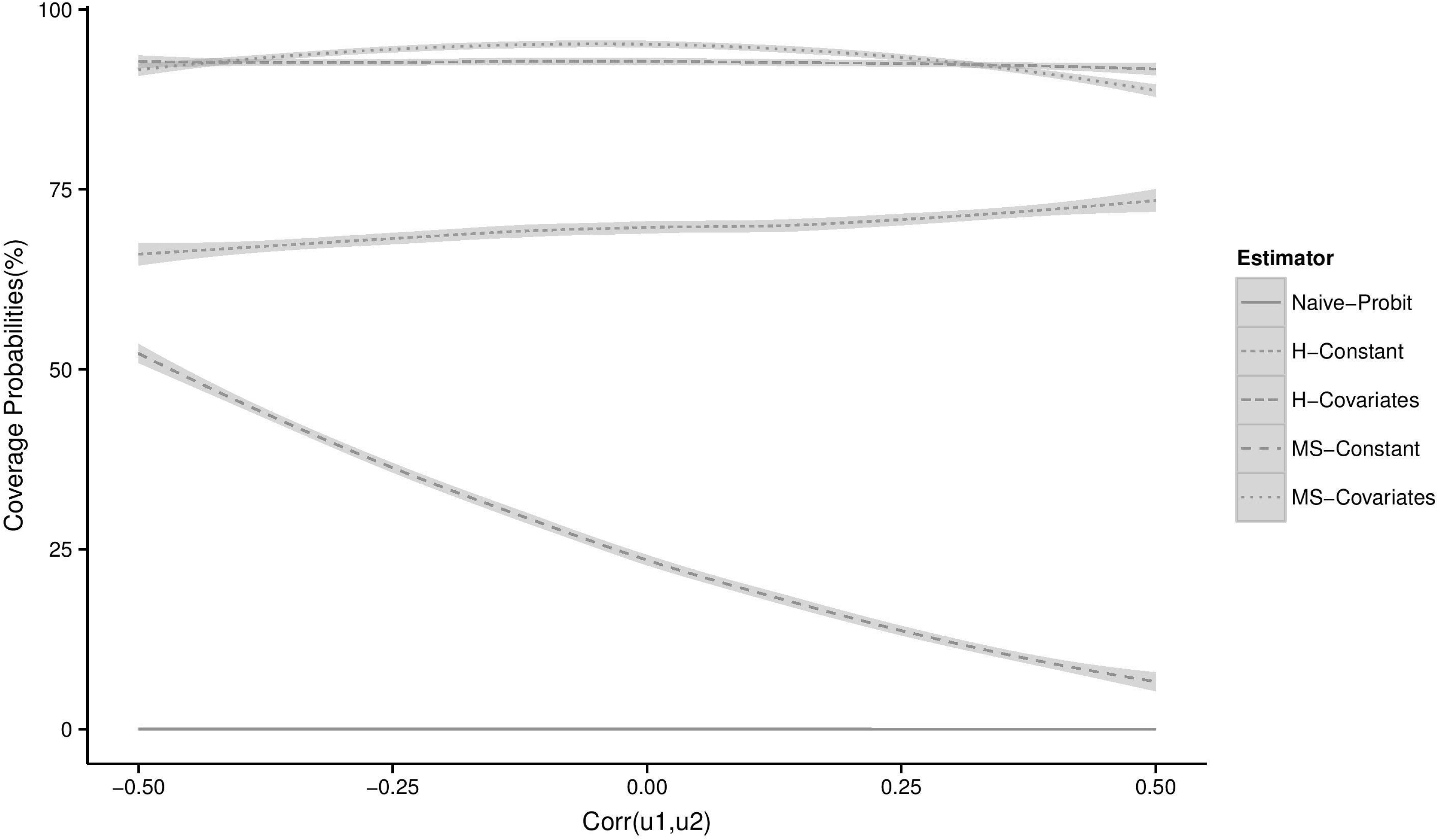
in increments of 0.02—capturing both strong negative correlation (i.e., sources purposefully report on distinct events) and strong positive correlation (i.e., sources purposefully report on the same events). The results are illustrated in Figure 1, which provides the CPs across these simulations.
Estimator Performance with source correlation. Curves are smoothed via LOESS. Points or non-smoothed lines render the same conclusions.

We see that our preferred method, Multi-source with Covariates, consistently performs well even despite omitted variables in the misclassification equations and high levels of correlation. With correlation between
 $-0.44$
and 0.3 it is the optimal estimator, bested only by the Hausman with Covariates when the level of correlation becomes very high. This is expected given that under these conditions, extremely high levels of correlation, there is less additional information from the second source—they converge toward one another. What is more notable is the persistent fitness of our estimator across all simulations, indicating that it is robust to typical violations of Assumption 1(a) one might observe in real-world data like that we consider in the next section.Footnote
21
5 State Repression in Africa
As discussed in the introduction, event-based data have been widely used in the literature on contentious politics. Misclassification is widely believed to be an issue in these studies, with researchers arguing that such “incorrect misclassification is likely to be systemic rather than random” (Schrodt Reference Schrodt2012, 557). That is, outcome data is likely to suffer from the type of error observed to generate substantial bias in our simulations. Notably, the literature on repression has generated theories predicting when and where we should be most likely to observe underreporting; arguing that high-visibility events occurring in urban centers of economically developed, less authoritarian regimes are more likely to be reported (Davenport Reference Davenport2007; Davenport and Ball Reference Davenport and Ball2002). Yet, much of the quantitative literature on repression fails to explicitly account for the potential bias introduced from underreporting in their statistical analysis. This motivates our current analysis, where we examine both: (i) the effect of misclassification on common predictors of repression and (ii) analyze whether we find support for those factors thought to produce reporting bias.
Specifically, we estimate a model of repression in Africa using the set of methods detailed in Section 4. Our outcome data is taken from SCAD (Salehyan et al. Reference Salehyan, Hendrix, Hamner, Case, Linebarger, Stull and Williams2012), which generates event data on forty-seven African countries using key word searches of Associated Press (AP) and Agence France-Presse (AFP) news wires. These data are particularly useful for our purposes in two ways. First, since 2012 events have been recorded as being reported by the AP, the AFP, or both—that is, there are multiple sources.Footnote 22 Second, the creators of this data set have discussed the likelihood of underreporting, utilizing a Lincoln–Peterson mark–recapture method to estimate that 24% of social conflict events go unreported (Hendrix and Salehyan Reference Hendrix and Salehyan2015).Footnote 23 While mark and recapture methods prove useful for diagnosing the presence of underreporting, they do not remedy the resulting bias in subsequent empirical analysis as we aim to do.Footnote 24
Therefore, using these data, we generate a binary outcome, Repression, which is coded as one if either or both of the news wires report on (lethal or nonlethal) repression initiated by the government or pro-government actors during a state–month, and zero otherwise. For the submodels in our misclassification estimator, we construct two additional binary variables, one for events reported by the AP and one for events reported by the AFP. Following the Poe and Tate (Reference Poe and Neal Tate1994) model, we believe repression should be increasing in population, and decreasing in democracy and GDP per capita.Footnote 25 We include each as independent variables, with coding and data sources elaborated in the Online Appendix. Lastly, our estimator requires additional covariates predicting misclassification, which is unrelated to the true-event probability. Hendrix and Salehyan (Reference Hendrix and Salehyan2016) have suggested that nonconflict related news reports may indicate the total amount of media effort devoted to a country and include a country-year average (divided into quantiles) as a control in their model. Drawing on this, we collect new data on the number of nonconflict related news reports for each country by the AP and AFP, respectively.Footnote 26 The values for each, AP Reports and AFP Reports, are introduced in the submodels predicting misclassification. Our expectation is that greater media effort (e.g., higher values) will be negatively associated with the probability of misclassification.
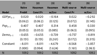
Model of repression in Africa.

Note: The estimators are the same as those used in the simulations and detailed in Section 4. The covariates are the log of GDP per capita (GDPpc), the log of population (Pop), and an indicator if the country is a democracy (Demo), each lagged by one period.
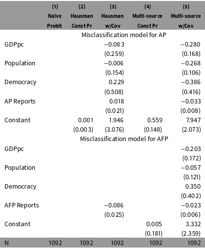
Models of reporting bias on repression in Africa.

Note: Results produced by the same models estimated in Table 3, partitioned for ease of exposition. AP Reports & AFP Reports are number of nonconflict news stories. To clarify the presentation: Model (1) produces no estimates of misclassification; Model (2) estimates a single misclassification probability, common to both sources; Model (3) estimates a misclassification model of the dependent variable, from either source, using the risk-model covariates and AP Reports & AFP Reports; Model (4) estimates separate, constant misclassification probabilities for the two sources; and Model (5) estimates separate misclassification models for the two sources.
The results from these models are presented in Tables 3 and 4. Table 3 shows the results from the repression model of each estimator, the outcome of primary theoretical interest in our illustration. Glancing across the table highlights both (i) the importance of accounting for misclassification and (ii) how one accounts for misclassification. With the Naïve Probit (Model 1), we see that both Pop and Demo are significant in their expected directions, with GDPpc positive and insignificant. The effect of GDPpc is inconsistent with the theoretical literature, however, it is not uncommon in the empirical literature to date.Footnote 27 We see that the results from the Hausman et al. (Reference Hausman, Abrevaya and Scott-Morton1998) estimator (Model 2) are nearly identical to those from the naïve probit in this analysis. This, despite the fact that theory would suggest, and the originators of the data set have concluded, that events go underreported in the data, that is, exactly the setting in which researchers would turn to this estimator.Footnote 28 The Multi-source Constant model also does not affect much change, with all results roughly the same as in Models 1 and 2.
None of this is surprising given that our belief is that the misclassification is systemic. As such, we turn to Models 3 and 5 where the misclassification probabilities are nonconstant, predicted by the same covariates included in the repression model. We see sizable differences in Model 3, Hausman with Covariates, with an increase in the constant offset by decreases in both Pop and Demo. That is, the base-line risk of repression is more likely than what is evidenced in our reported sample due to misclassification, which also appears to have biased the effect of the predictors. Similar, if more pronounced, results are found in Model 5, our Multi-source with Covariates model, with fairly dramatic shifts to all three predictors and the constant. Most notably, GDPpc becomes negative and is now statistically significant, consistent with theoretical expectations. We also see the negative effect of Demo increases and the positive effect of Pop increases. What does this mean? It suggests misclassification was biasing the effect of GDPpc, Pop, Demo as repression in wealthy, populous democracies is more likely to be reported on, causing us to erroneously conclude that repression is actually more likely in those environments than it is.Footnote 29
We can examine these causes of reporting bias more explicitly in Table 4, which provides the misclassification probabilities (and models) where they are estimated.Footnote 30 Focusing on Model 5, we observe two main findings of note: first, the AP is more likely to suffer from underreporting than AFP, as indicated by their constants; second, our measures for “media effort” are significantly and negatively related to misclassification, that is, the more nonviolent news stories reported on a region by the AP and AFP, the more likely they are to accurately report an incident of repression. We do not find significant support for the repression-model predictors in this analysis, however, given that these should predict media effort, not just misclassification, this null finding makes sense as we already account for media effort explicitly as an additional predictor.
6 Applications & Extensions
To introduce and describe our approach we have focused our discussion on fixed observational units with only two binary-event indicators (e.g., reports) of a binary outcome, however, particular applications of concern to applied researchers may deviate from this in several ways. Therefore, we detail some of the more likely departures here and discuss how our method can be utilized under a variety of these contexts.
First, data are often compiled from more than two underlying sources. As alluded to in footnote 9, our method can be easily amended to handle these additional sources by simply expanding the joint likelihood. In the most general setting, suppose that there are
 $M({\geqslant}2)$
reporting sources. Let the binary-outcome variable from the
 $j$
th source be
 $\boldsymbol{Y}_{j}$
,
 $j=1,\ldots ,M$
, and
 $\boldsymbol{Y}_{\text{T}}$
be the true indicator of an event. Let
 $\boldsymbol{X}$
be a covariate that is associated with the true-event indicator, and
 $\boldsymbol{Z}_{1},\ldots ,\boldsymbol{Z}_{M}$
be the source-specific covariates. Maintaining all earlier assumptions, define source-specific false negative probabilities,
 $\unicode[STIX]{x1D6FC}_{j}(\boldsymbol{X},\boldsymbol{Z}_{j})=\text{pr}(\boldsymbol{Y}_{j}=0|\boldsymbol{Y}_{\text{T}}=1,\boldsymbol{X},\boldsymbol{Z}_{j})$
, for
 $j=1,\ldots ,M$
, and
 $\text{pr}(\boldsymbol{Y}_{\text{T}}=1|\boldsymbol{X})=F(\boldsymbol{X},\unicode[STIX]{x1D6FD})$
. Then the joint probability of
 $\boldsymbol{Y}_{1},\ldots ,\boldsymbol{Y}_{M}$
given
 $\boldsymbol{X}$
,
 $\boldsymbol{Z}_{1},\ldots ,\boldsymbol{Z}_{M}$
is
 $$\begin{eqnarray}\displaystyle & & \displaystyle \text{pr}(\boldsymbol{Y}_{1}=y_{1},\ldots ,\boldsymbol{Y}_{M}=y_{M}|\boldsymbol{X},\boldsymbol{Z}_{1},\ldots ,\boldsymbol{Z}_{M})\nonumber\\ \displaystyle & & \displaystyle \quad =\text{pr}(\boldsymbol{Y}_{1}=y_{1},\ldots ,\boldsymbol{Y}_{M}=y_{M}|\boldsymbol{Y}_{\text{T}}=0,\boldsymbol{X},\boldsymbol{Z}_{1},\ldots ,\boldsymbol{Z}_{m})\text{pr}(\boldsymbol{Y}_{\text{T}}=0|\boldsymbol{X},\boldsymbol{Z}_{1},\ldots ,\boldsymbol{Z}_{M})\nonumber\\ \displaystyle & & \displaystyle \qquad +\,\text{pr}(\boldsymbol{Y}_{1}=y_{1},\ldots ,\boldsymbol{Y}_{M}=y_{M}|\boldsymbol{Y}_{\text{T}}=1,\boldsymbol{X},\boldsymbol{Z}_{1},\ldots ,\boldsymbol{Z}_{m})\text{pr}(\boldsymbol{Y}_{\text{T}}=1|\boldsymbol{X},\boldsymbol{Z}_{1},\ldots ,\boldsymbol{Z}_{M})\nonumber\\ \displaystyle & & \displaystyle \quad =\{1-F(X,\unicode[STIX]{x1D6FD})\}I(y_{1}=\cdots =y_{M}=0)\nonumber\\ \displaystyle & & \displaystyle \qquad +\,\unicode[STIX]{x1D6FC}_{1}^{1-y_{1}}(\boldsymbol{X},\boldsymbol{Z}_{1})\{1-\unicode[STIX]{x1D6FC}_{1}(\boldsymbol{X},\boldsymbol{Z}_{1})\}^{y_{1}}\times \cdots \times \unicode[STIX]{x1D6FC}_{M}^{1-y_{M}}(\boldsymbol{X},\boldsymbol{Z}_{M})\{1-\unicode[STIX]{x1D6FC}_{M}(\boldsymbol{X},\boldsymbol{Z}_{M})\}^{y_{M}}F(\boldsymbol{X},\unicode[STIX]{x1D6FD}),\nonumber\end{eqnarray}$$
for
 $y_{j}=\{0,1\}$
and
 $j=1,\ldots ,M$
. Therefore, the likelihood function of the observed data over
 $N$
independent observations is
 $$\begin{eqnarray}\displaystyle L & = & \displaystyle \prod \left[\{1-F(\boldsymbol{X},\unicode[STIX]{x1D6FD})\}I(y_{1}=\cdots =y_{M}=0)\right.\nonumber\\ \displaystyle & & \displaystyle +\left.\unicode[STIX]{x1D6FC}_{1}^{1-y_{1}}(\boldsymbol{X},\boldsymbol{Z}_{1})\{1-\unicode[STIX]{x1D6FC}_{1}(\boldsymbol{X},\boldsymbol{Z}_{1})\}^{y_{1}}\times \cdots \times \unicode[STIX]{x1D6FC}_{M}^{1-y_{M}}(\boldsymbol{X},\boldsymbol{Z}_{M})\{1-\unicode[STIX]{x1D6FC}_{M}(\boldsymbol{X},\boldsymbol{Z}_{M})\}^{y_{M}}F(\boldsymbol{X},\unicode[STIX]{x1D6FD})\right],\nonumber\end{eqnarray}$$
where the outer product is over
 $N$
. As always, the maximum likelihood estimator of the model parameters can be obtained by maximizing the logarithm of
 $L$
.Footnote
31
This shows how our estimation strategy can easily be tailored for a general number of sources (e.g., 3, 5, 8 …) in a straightforward way. However, some event data sets are compiled from hundreds or even thousands of sources (e.g., ICEWS, GDELT, Phoenix), which would tax our method and result in a badly behaved likelihood; as the information in each “cell” of the joint likelihood becomes increasingly small. A partial solution for these data may be to classify the many sources into fewer clusters (e.g., international news agencies, national newspapers, local newspapers) which share common, within-cluster, features in the scope and nature of their coverage. Then it is reasonable to assume that the misclassification probabilities vary across the clusters but not much within a cluster, reducing the number of parameters and permitting estimation as before.
As an example, consider the Armed Conflict Location & Event Dataset (ACLED), a widely used dataset on substate violent events.Footnote
32
These data are drawn from a variety of sources—ranging between 70 and 232 sources from 1997 to 2012—which, at first pass, might suggest that our approach is not feasible. However, the top-10 sources account for nearly three-fourths of the events in the dataset, suggesting diminishing returns from the collection of the additional
 $220+$
sources.Footnote
33
In contexts where the collection of these additional sources of data is more costly or onerous, there is a value in constraining the number of sources and then employing a statistical correction such as ours. Additionally, the reporting sources naturally classify into three types (i.e., international, national, and regional), with the total number of sources in each African country varying from 8 to 100. We believe it is reasonable to think of each reporting type as a “macro-source” with common misclassification probabilities. For example, as in our paper, international sources are likely to be affected by the amount of reporting coverage generally on a state and the distance to a bureau office. Whereas whether any regional sources reported a true event is more likely to be a function of the number of such sources available to ACLED for that state, which vary considerably, and the degree of press freedom in that state. Considered in this way, we have three observed “reports”—
 $Y_{\mathit{INT}}=I(Y_{\mathit{int}1}+\cdots +Y_{\mathit{int}K}\geqslant 1)$
,
 $Y_{\mathit{NAT}}=I(Y_{\mathit{nat}1}+\cdots +Y_{\mathit{nat}K}\geqslant 1)$
, and
 $Y_{\mathit{REG}}=I(Y_{\mathit{reg}1}+\cdots +Y_{\mathit{reg}K}\geqslant 1)$
—each with respective misclassification probabilities—
 $\unicode[STIX]{x1D6FC}_{\mathit{INT}}=\unicode[STIX]{x1D6F7}(X,\mathit{Dist},\mathit{Coverage})$
,
 $\unicode[STIX]{x1D6FC}_{\mathit{NAT}}=\unicode[STIX]{x1D6F7}(X,\mathit{No.~of~National~Sources},\mathit{Press~Freedom})$
,
 $\unicode[STIX]{x1D6FC}_{\mathit{REG}}=\unicode[STIX]{x1D6F7}(X,\mathit{No.~of~Regional~Sources},\mathit{Press~Freedom})$
. Estimation would then proceed as given in the three-source variation of the likelihood detailed above.Footnote
34
Beyond the issues on the number of reporting sources, the questions asked by researchers using media-reported event data may differ from what we have introduced here. First, researchers may be interested in event counts (e.g., the number of protests, terrorist attacks, human rights violations), rather than the binary outcomes we consider here. The derivation of our method above does not apply to these applications, however, our basic likelihood framework could be used to address such problems. That is, given a parametric model for the true-event-generating process—which we often assume in political science—and a parametric model for the misclassification, we can form the likelihood function of the observed data. Let
 $\boldsymbol{Y}$
,
 $\boldsymbol{Y}_{T}$
and
 $\boldsymbol{X}$
be the reported count, true count, and a set of covariates, respectively. Let
 $p(y_{\text{T}}|\boldsymbol{X},\unicode[STIX]{x1D6FD})=\text{pr}(\boldsymbol{Y}_{\text{T}}=y_{\text{T}}|\boldsymbol{X},\unicode[STIX]{x1D6FD})$
be the true data-generating model and
 $m(y|y_{\text{T}},\boldsymbol{X})=\text{pr}(\boldsymbol{Y}=y|\boldsymbol{Y}=y_{\text{T}},\boldsymbol{X},\unicode[STIX]{x1D6FE})$
be the model for misclassification. Then one can form an induced model for the reported response
 $\boldsymbol{Y}$
given
 $\boldsymbol{X}$
,
 $\text{pr}(\boldsymbol{Y}=y|\boldsymbol{X},\unicode[STIX]{x1D6FD},\unicode[STIX]{x1D6FE})=\sum _{y_{\text{T}}}m(y|y_{\text{T}},\boldsymbol{X},\unicode[STIX]{x1D6FE})p(y_{\text{T}}|\boldsymbol{X},\unicode[STIX]{x1D6FD})$
, write the likelihood, and proceed for estimation of
 $\unicode[STIX]{x1D6FD}$
, the main model parameters.Footnote
35
Second, researchers may be interested in using media-based data when determining the sample itself (e.g., studies on the duration of conflicts, whether protests turn violent). In these analyses, underreporting would result in sample-selection bias—a failure to include a set of true observations in the sample—rather than, or in addition to, misclassification in the outcome. As discussed and presented here our method does not readily address this issue, it is better suited for analyses with fixed observational units. However, despite the well-known methods for handling selection, both generally and with binary-outcome data (Maddala Reference Maddala1983; Heckman Reference Heckman1977), none deals with the multiple source issue we have discussed here. As such, we are currently working on a multi-source selection model which would allow for researchers to address these problems.
7 Conclusion
Traditionally researchers devote less attention to measurement error in the outcome, however, here we have highlighted the severity of the bias induced by differential misclassification in binary outcomes. Our simulations show that misclassification can produce substantial bias when researchers employ either: (i) strategies which assume no misclassification or (ii) strategies which assume nondifferential misclassification. Further, we show that unbiased estimates can only be obtained by directly estimating a model of misclassification and weighting the risk-model probabilities accordingly.
The threat of systematic measurement error from underreporting is widely discussed in applied research using media-generated event data, yet little work has proposed general strategies to remedy this potential bias.Footnote 36 We show how researchers possessing more than one source of data-generating information can achieve this desired result. Specifically, we derive an estimator for applications in which researchers have at least two sources of potentially misclassified data on a single outcome of interest. Under few assumptions, our estimator returns unbiased estimates of the risk probability and allows for source-specific misclassification estimates.
Specifically, we have focused on how our strategy can aid researchers using event-based data comprised from multiple reporting outlets. To our knowledge, no current estimator—in political science, sociology, economics, or statistics—accommodates both multiple sources of reporting data and potential misclassification.Footnote 37 Given that many of the first wave of recommendations to ameliorate reporting bias consisted of gathering data from additional sources, our estimators should reflect this feature of the data-generating process. Yet, as we note, even additional sources are unlikely to result in an uncontaminated data set, meaning that further statistical corrections for misclassification will often be required. As such, we provide a unified method suited for multiple sources of potentially misclassified data. The results show the fitness of our estimator under either differential or nondifferential misclassification, suggesting it could be preferred as a general method when researchers are unaware of the nature of the misclassification in their data.
We illustrated the utility of this method in a model of state repression in Africa, observing that predictor effects change dramatically when misclassification is ignored. We believe that similar results will be obtained when researchers utilize our method in studies of protest behavior, civil war, political violence, and so forth. In future research, we plan to extend on the method introduced here in two ways. First, deriving a semiparametric efficient estimator for the class of problems outlined above. Second, consider cases where the sample itself is defined by potentially misclassified event-based data (e.g., protests, politically excluded ethnic groups).
Funding
This work was supported by a grant from the National Cancer Institute [U01-CA057030 to R.J.C.] and a post-doctoral fellowship from Conselho Nacional de Desenvolvimento Científico e Tecnológico [201192/2015-2 to B.B.].
Supplementary material
For supplementary material accompanying this paper, please visit https://doi.org/10.1017/pan.2016.13.