





1 Introduction
Exploratory multidimensional item response theory (MIRT; Reckase, Reference Reckase2009), also known as exploratory item factor analysis (IFA; Bock & Schilling, Reference Bock and Schilling1997; Bock et al., Reference Bock, Gibbons and Muraki1988), has become a foundational framework for exploring complex latent structures underlying item response data. However, estimating MIRT models in large-scale high-dimensional (i.e., the dimension of the latent space is highFootnote 1 ) settings, where the number of respondents, items, or factors may all be considerable, remains challenging. These challenges are two-fold. Firstly, in high-dimensional settings, the estimation of the underlying MIRT model is computationally intensive or even infeasible for most existing methods (Chen & Zhang, Reference Chen and Zhang2021; Chen et al., Reference Chen, Li and Zhang2019). Secondly, to achieve interpretable factor structures when many items and many factors are involved, the importance of finding solutions having simple-structured loading matrices significantly grows, leading to more complexity in suitable regularized methods targeting such sparsity.
In the past, several estimation methods and related algorithms have been proposed. The most commonly studied methods include marginal maximum likelihood estimation (MMLE), which has long been used in IFA literature to fit MIRT models with many factors (Bock & Aitkin, Reference Bock and Aitkin1981). MMLE requires one to integrate out latent variables to obtain the marginal likelihood function, and the expectation–maximization algorithm is commonly utilized for estimation. The biggest computational challenge for MMLE-based methods lies in approximating high-dimensional integrals with respect to latent variables. Several algorithms have been designed and studied in simulations to address this problem. In particular, the recently proposed regularized variational estimation MIRT (VEMIRT) method exhibits a significant computational improvement compared to existing methods (Cho et al., Reference Cho, Xiao, Wang and Xu2024). In addition, a stochastic proximal framework, which was proposed by Zhang and Chen (Reference Zhang and Chen2022), demonstrated its capability to deal with larger datasets and more complex factor structures. However, the size of the datasets generated in both of their simulation studies was restricted, and the number of factors did not exceed 5. As we will show further on in this article, the improved MMLE-based methods are limited in handling larger datasets and more complex factor structures. We note that scalable deep-learning-based alternatives have also been proposed (Converse et al., Reference Converse, Curi, Oliveira and Templin2021; Luo & Ji, Reference Luo and Ji2025; Urban & Bauer, Reference Urban and Bauer2021), but a detailed examination of such approaches is beyond the scope of the present study.
In contrast, although computationally efficient, joint maximum likelihood estimation (JMLE; Embretson & Reise, Reference Embretson and Reise2013) has historically received limited attention due to concerns about its statistical inconsistency. Unlike MMLE, JMLE treats latent variables as fixed effects and begins by estimating latent scores and item parameters jointly. Consequently, the number of parameters to be estimated increases with the sample size, and this is a well-known irregularity condition for MLE that leads to statistical inconsistency (Andersen, Reference Andersen1973; Ghosh, Reference Ghosh1995; Haberman, Reference Haberman1977; Neyman & Scott, Reference Neyman and Scott1948). However, in large-scale settings where both the sample size and the number of items can be large, Chen et al. (Reference Chen, Li and Zhang2019) proved the statistical consistency of JML estimators. By implementing a projected gradient descent algorithm, they demonstrated the remarkable computational efficiency of the JML estimation method. Despite the simplicity of implementation and the computational power of JMLE-based methods in large-scale MIRT estimation, the algorithm may benefit from further improvements at the computational level and various regularization extensions. However, progress in this direction remains limited, and that is where our study departs.
A primary concern regarding Chen et al.’s (Reference Chen, Li and Zhang2019) work is the use of factor rotation to reach interpretable factor solutions. Rotation is widely used in exploratory factor analysis to achieve sparse/simple loading structures for interpretational purposes. Although rotation has long been standard practice in the field, it is not without limitations. First, because it can only generate a rotated loading matrix with many small nonzero elements, an extra step of arbitrary thresholding must be followed to decide which near-zero loadings can be ignored and regarded as effectively zero. In a similar context of extracting principal components, this method has been pointed out to be misleading, as an alternative subset of variables could provide a better approximation of the data (Cadima & Jolliffe, Reference Cadima and Jolliffe1995). Moreover, the wide range of available rotation techniques complicates practice, since no single method is universally acknowledged as superior (Scharf & Nestler, Reference Scharf and Nestler2019). Alternatively, more stable and objective solutions can be obtained by regularized methods that force the loading matrix to be sparse or simple-structured by, for example, imposing a penalty on it. The potential of regularized methods, in the same context of extracting principal components, has been validated by Guerra-Urzola et al. (Reference Guerra-Urzola, Van Deun, Vera and Sijtsma2021) through simulation studies. Unfortunately, the development of regularized methods in JMLE literature is less mature than in MMLE. For example, Sun et al. (Reference Sun, Chen, Liu, Ying and Xin2016) first proposed a least absolute shrinkage and selection operator (lasso) penalized MIRT method that imposes the
$\ell _1$
 penalty on the marginal likelihood function to achieve sparsity in loading matrices. Similarly, Beisemann et al. (Reference Beisemann, Holling and Doebler2025) developed a regularized MMLE-based method for multidimensional count data item response models. More generally, existing MMLE-based approaches, including VEMIRT and the stochastic proximal framework, allow an
$\ell _1$
 penalty to be imposed on the objective function to obtain sparse and interpretable loading structures. In summary, the use of penalized MLE by adding, for example, the lasso, represents a parallel and conceptually distinct alternative to traditional rotation techniques for achieving a simple/sparse loading structure (Goretzko, Reference Goretzko2023; Scharf & Nestler, Reference Scharf and Nestler2019) and remains to be developed for the JML estimation method.
However, given the NP-hardness of optimal subset selection (Natarajan, Reference Natarajan1995), the lasso, as the most widely implemented penalized method, has been suggested only as a heuristic approach because it cannot guarantee the best subset recovery unless stringent conditions on the data hold (Bertsimas et al., Reference Bertsimas, King and Mazumder2016; Tibshirani, Reference Tibshirani2011, pp. 277–278), which might not be the case in the real world. Moreover, the lasso is a penalized estimation approach that introduces a trade-off between bias and variance. While it improves model sparsity and generalization, it tends to suffer from shrinkage-induced bias, especially for large coefficients, as estimates are pulled toward zero (Hastie et al., Reference Hastie, Tibshirani and Friedman2009), and it was also highlighted in Beisemann et al. (Reference Beisemann, Holling and Doebler2025) for count data IRT. A different approach to enforcing sparse solutions is by imposing cardinality constraints on the model coefficients. Optimization under cardinality constraints has led to substantial progress in solving the sparse linear regression problem when the number of predictors is large (Bertsimas et al., Reference Bertsimas, King and Mazumder2016; Bertsimas & Van Parys, Reference Bertsimas and Van Parys2020). This cardinality-constrained approach has been further implemented for sparse exploratory factor analysis (Lê et al., Reference Lê, Vermunt and Van Deun2024), through which one can obtain unpenalized sparse loading matrices by directly specifying the expected number of nonzero loadings. Previous simulation studies have already revealed the potential of the cardinality-constrained approach in the context of regression (Adachi & Kiers, Reference Adachi and Kiers2017; Bertsimas et al., Reference Bertsimas, King and Mazumder2016) and principal component analysis (PCA; Guerra-Urzola et al., Reference Guerra-Urzola, de Schipper, Tonne, Sijtsma, Vera and Van Deun2023). However, to the best of our knowledge, this approach has not yet been generalized into high-dimensional MIRT models estimation.
Estimating MIRT models by integrating JMLE with the cardinality-constrained approach is not straightforward because previous cardinality-related research mostly focused on problems that can be solved by least squares optimization routines, while in JMLE, one needs to minimize a logarithmic logistic likelihood function. To solve the issue, we propose a minimization–majorization (MM) algorithm (Lange, Reference Lange2004; Lange et al., Reference Lange, Hunter and Yang2000) to connect the logarithmic logistic likelihood function with the cardinality-constrained approach (Adachi & Trendafilov, Reference Adachi and Trendafilov2016). We may add that a similar approach was proposed more than a decade ago in logistic PCA research (De Leeuw, Reference De Leeuw2006; Lee et al., Reference Lee, Huang and Hu2010) but has never been extended to exploratory MIRT approaches. As will be explained in Section 2 below, with the help of the MM algorithm, the JMLE objective can be efficiently optimized using an iterative alternating least squares routine. Consequently, the MM algorithm not only offers a suitable framework to accommodate the cardinality-constrained approach but also improves general computational efficiency for other regularized approaches, such as the lasso, that are built on it.
Although the cardinality-constrained approach and the lasso-penalized approach serve similar aims, their combination may still offer complementary benefits in data analytic practice, as will be further elaborated in section 4. Therefore, we propose two regularized high-dimensional MIRT estimation algorithms tailored for large-scale item response data: (i) a lasso-penalized approach named lasso HiMIRT, incorporated with the alternating optimization–alternating direction method of multipliers (AO-ADMM) framework (Huang et al., Reference Huang, Sidiropoulos and Liavas2016) and (ii) a cardinality-constrained approach, named card HiMIRT, through which one can enforce sparsity by specifying the number of nonzero elements in the loading matrix. We will show how the two approaches can be used in conjunction for optimally exploring real data using MIRT models. The source code and examples of the proposed methods can be found in https://github.com/DogeinSky/HiMIRT.
The article is organized as follows. Section 2 introduces the problem setup and explains the majorization of the model objective by the MM algorithm. The alternating optimization framework utilized in the proposed estimation algorithms is introduced in Section 3, followed by an introduction to the model selection strategies in Section 4. In Section 5, three simulation studies that assess the performance of our methods and compare them with related methods are presented. Additionally, the evaluation of the model selection strategies is also included in Section 5. Section 6 illustrates the proposed approaches using a real data example. Finally, Section 7 discusses the limitations of the current work and suggests directions for future research.
2 Model objective and problem setup
2.1 Notation
We first introduce some general notation rules. Matrices are denoted by bold uppercase, and the transpose of a matrix is indicated by the superscript
$\text {T}$
 , for example,
$\mathbf {A}^{\text {T}}$
 . Column vectors are denoted by bold lowercase, row vectors by bold lowercase with the transpose sign, and scalars by lowercase italics. Especially,
$\mathbf {1}_N$
 denotes an N-vector with all components equal to 1. Given an n-vector
$\mathbf {x}$
 , the
$\ell _0$
 -norm
$\|\mathbf {x}\|_0=\sum _{i=1}^{n} I(x_i \neq 0)$
 is the cardinality (i.e., the number of nonzero elements) of
$\mathbf {x}$
 , where the indicator function
$I(x_i \neq 0)$
 takes the value 1 if
$x_i$
 is nonzero, and otherwise 0.
$\|\mathbf {x}\|_1=\sum _{i=1}^{n} |x_i|$
 defines the
$\ell _1$
 -norm of
$\mathbf {x}$
 , and
$|\cdot |$
 takes the absolute value of an element. The same notation also applies to the
$\ell _0$
 -norm and
$\ell _1$
 -norm of a
$J \times K$
 matrix
$\mathbf {A}$
 , denoted by
$\|\mathbf {A}\|_0=\sum _{j=1}^{J}\sum _{k=1}^K I(a_{jk}\neq 0)$
 and
$\|\mathbf {A} \|_1=\sum _{j=1}^{J}\sum _{k=1}^K|a_{jk}|$
 . Furthermore,
$\|\mathbf {x}\|_2=\sqrt {\sum _{i=1}^{n} x_i^2}$
 defines the Euclidean norm of
$\mathbf {x}$
 , while
$\|\mathbf {A}\|_F=\sqrt {\sum _{j=1}^{J}\sum _{k=1}^{K} a_{jk}^2}$
 represents the Frobenius norm of a
$J \times K$
 matrix
$\mathbf {A}$
 .
2.2 MIRT models for dichotomous responses
This article focuses on a class of two-parameter MIRT models. Specifically, we consider a binary response matrix
$\mathbf {Y}$
 of size
$N \times J$
 , where
$y_{ij} \in \{0,1\}$
 indicates the response of respondent
$i = 1, \ldots , N$
 to item
$j = 1, \ldots , J$
 . The model involves three sets of parameters: the
$N \times K$
 latent variable matrix
$\boldsymbol {\Theta }=(\boldsymbol {\theta }_1, \dots , \boldsymbol {\theta }_N)^{\text {T}}$
 , the
$J \times K$
 item loading matrix
$\mathbf {A}=(\mathbf {a}_1,\dots ,\mathbf {a}_J)^{\text {T}}$
 , and the J-dimensional item difficulty vector
$\mathbf {d}=(d_1, \ldots , d_J)$
 . K denotes the number of latent variables. Each respondent’s latent score vector is denoted by
$\boldsymbol {\theta }_i = (\theta _{i1}, \ldots , \theta _{iK})$
 , and each item’s loading vector is
$\mathbf {a}_j = (a_{j1}, \ldots , a_{jK})$
 with corresponding difficulty parameter
$d_j$
 . Note that the latent vectors
$\boldsymbol {\theta }_i$
 correspond to the rows of
$\boldsymbol {\Theta }$
 , whereas the latent variables correspond to the columns of
$\boldsymbol {\Theta }$
 , denoted
$\boldsymbol {\Theta }_{[k]}$
 for the kth variable. The probability of a correct response (i.e., observing the corresponding random variable
$Y_{ij} = 1$
 ) is modeled as

where
$f: \mathbb {R} \rightarrow \mathbb {R}$
 is a prespecified link function. A common choice is the logistic link function for the M2PL model (Reckase, Reference Reckase2009, p. 86):

For the normal ogive model (Reckase, Reference Reckase2009, p. 95), the link function becomes

where
$\phi (x)$
 is the probability density function of the standard normal distribution. For simplicity, we adopt a simplified expression of (2.1) from now on:

Two remarks are in order. First, for convenience, all methods in this article are built on the M2PL model, but everything discussed also applies to the normal ogive model. Second, a standard assumption in (M)IRT modeling is the local independence assumption, which states that given the latent vector
$\boldsymbol {\theta }_i$
 , respondent i’s responses
$Y_{i1},\ldots ,Y_{iJ}$
 are assumed to be conditionally independent. As a consequence, the probability of observing Y given
$\boldsymbol {\theta }$
 is the product of the individual M2PL response probabilities in (2.2).
2.3 Majorizing the model objective by MM numerical procedure
Chen et al. (Reference Chen, Li and Zhang2019) proposed a constrained JMLE framework to solve (2.2), which is computationally superior to MMLE in large-scale settings. While MMLE regards
$\boldsymbol {\theta }_i$
 s as random but missing vectors to be integrated out of the likelihood function, JMLE treats them as fixed effects and estimates them jointly with the item parameters. Hence, the objective function is maximized by finding optimal values for both the person parameters
$\boldsymbol {\Theta }$
 and item parameters
$\mathbf {A}$
 and
$\mathbf {d}$
 . To move toward a regularized extension of the JMLE framework, the incorporation of the MM algorithm offers a particularly effective strategy.
Based on the model (2.2) and the local independence assumption, we start from the joint log-likelihood function:

Because
$f(-x)=1-f(x)$
 and
$y_{ij} \in \{0,1\}$
 , by setting
$q_{ij}=2y_{ij}-1$
 , the log-likelihood function simplifies to

Maximizing the log-likelihood in (2.4) is equivalent to minimizing the negative log-likelihood. In this minimization setting, the MM algorithm constructs a simpler surrogate function that majorizes the original objective function and touches it at the supporting point. Iteratively updating the supporting point by the minimum of the majorizing function leads to a non-increasing sequence of loss values. For those readers who are not familiar with the MM algorithm, a helpful tutorial paper can be found in Lange (Reference Lange2004). In the following theorem, we introduce a quadratic upper bound for the log-likelihood objective (2.4).
Theorem 1. Let
$d_j^{(m)}, \boldsymbol {\theta }_i^{(m)}, \text { and } \mathbf {a}_j^{(m)}$
 represent the parameter values/vectors obtained in the mth iteration (similarly,
$\boldsymbol {\Theta }^{(m)},\mathbf {A}^{(m)}$
 , and
$\mathbf {d}^{(m)}$
 represent the parameter vectors/matrices computed in the mth iteration), so
$x_{ij}^{(m)}=d_j^{(m)}+\boldsymbol {\theta }_i^{(m)\text {T}}\mathbf {a}_j^{(m)}$
 . Define
$z_{ij}^{(m)} := x_{ij}^{(m)}-q_{ij}\frac {h(q_{ij}x_{ij}^{(m)})}{w(q_{ij}x_{ij}^{(m)})}$
 , where
$h(x) := -\frac {\mathrm {d} \log f(x)}{\mathrm {d} x}$
 is the first derivative of
$-\log f(x)$
 , and
$w(x)$
 can be either a constant
$\frac {1}{4}$
 or
$\frac {1-2f(x)}{2x}$
 for uniform majorization or non-uniform majorization, respectively. The inequality below always holds:

and the equality sign holds when
$\boldsymbol {\Theta }=\boldsymbol {\Theta }^{(m)},\mathbf {A}=\mathbf {A}^{(m)}$
 , and
$\mathbf {d}=\mathbf {d}^{(m)}$
 (see the proof in the Supplementary Material).
By Theorem 1, the majorizing function used in the (
$m+1$
 )th iteration of the algorithm is constructed on the right-hand side of the inequality in (2.5). The first two terms are constants, as they depend only on values from the previous iteration. Therefore, minimizing the right-hand side reduces to minimizing the third term, which is equivalent to the unweighted sum of squared terms if the uniform majorization is adopted. As a result, the MM algorithm allows converting the original objective of (2.4) into a least squares-like objective. Based on that, to minimize (2.4), the problem in each (
$m+1$
 )th iteration reduces to the following minimization problem:

where
$\mathbf {X}=\mathbf {1}_N\mathbf {d}^{\text {T}}+\boldsymbol {\Theta }\mathbf {A}^{\text {T}}$
 , and
$\mathbf {Z}^{(m)}$
 represents an
$N \times J$
 matrix consisting of
$z_{ij}^{(m)}$
 components. To address scale indeterminacy, the two equality constraints restrict the mean and variance of all latent variables to be 0 and 1, respectively.
Notice that after solving for the scale indeterminacy, the problem (2.6) is still subject to rotational indeterminacy. It can be shown that given any
$K \times K$
 orthogonal rotation matrix
$\mathbf {R}$
 , by defining
$\tilde {\boldsymbol {\Theta }}=\boldsymbol {\Theta }\mathbf {R}$
 and
$\tilde {\mathbf {A}}=\mathbf {AR}$
 as the rotated latent matrix and rotated loading matrix, the problem (2.6) is invariant under the rotation (i.e., the objective value does not change) because
$\tilde {\boldsymbol {\Theta }}\tilde {\mathbf {A}}^{\text {T}}=\boldsymbol {\Theta }\mathbf {R}\mathbf {R}^{\text {T}}\mathbf {A}=\boldsymbol {\Theta }\mathbf {A}^{\text {T}}$
 . In traditional exploratory factor analysis, rotational indeterminacy is solved by rotating the final loadings to a solution that best approximates a simple structure (Browne, Reference Browne2001). In our approach, the rotational indeterminacy is solved by imposing an
$\ell _1$
 penalty, or by constraining the cardinality of the loading matrix, as described below.

Although an orthogonal/oblique rotation keeps
$\frac {1}{8} \| \mathbf {Z}^{(m)} - \mathbf {X} \|_F^2$
 invariant, it is very unlikely that
$\lambda \|\mathbf {A} \|_1$
 or
$\|\mathbf {A} \|_0$
 stays the same. Consequently, the proposed methods are rotation-free and still result in sparse/simple structures in the loading matrix.
To solve the two problems, the parameter set
$(\mathbf {d},\boldsymbol {\Theta },\mathbf {A})$
 can be split into
$(\mathbf {d},\boldsymbol {\Theta })$
 and
$\mathbf {A}$
 , and an alternating optimization framework can be employed. Specifically, in each iteration, we first update
$(\mathbf {d},\boldsymbol {\Theta })$
 . Next, given the updated
$(\mathbf {d},\boldsymbol {\Theta })$
 , we use ADMM to update
$\mathbf {A}$
 for the lasso-penalized problem. For the cardinality-constrained problem, the update step for
$\mathbf {A}$
 simplifies to a straightforward sorting procedure following several mathematical transformations. We now turn to the more technical details of the alternating optimization framework.
3 Alternating optimization framework
In this section, the proposed algorithms are introduced based on the well-established alternating least squares framework (Ten Berge, Reference Ten Berge1993). Specifically, each iteration begins with updating the difficulty vector
$\mathbf {d}$
 and the latent matrix
$\boldsymbol {\Theta }$
 . The subsequent update of the loading matrix
$\mathbf {A}$
 differs depending on whether an
$\ell _1$
 penalty or a cardinality constraint is used. The structure of the following sections mirrors this organization.
3.1 Update the difficulty vector
$\mathbf {d}$
 and the latent matrix
$\boldsymbol {\Theta }$


By setting
$\frac {\partial \frac {1}{8}\|\mathbf {Z}^{(m+1)}-\mathbf {X} \|_F^2}{\partial \mathbf {d}}=0$
 , the analytical solution of
$\mathbf {d}$
 can be derived as

where
$\mathbf {Q}=2\mathbf {Y}-\mathbf {1}_{N\times J}$
 , and
$\mathbf {H}^{(m+1)}$
 is an
$N \times J$
 matrix with
$h(q_{ij}x_{ij}^{(m+1)})$
 on the ith row and jth column, and
$\odot $
 is the Hadamard/element-wise product. After obtaining
$\mathbf {d}^{(m+1)}$
 , by introducing
$\mathbf {Z}^{\dagger (m+1)}=\mathbf {Z}^{(m+1)}-\mathbf {d}^{(m+1)}$
 , we can obtain
$\|\mathbf {Z}^{\dagger (m+1)}-\boldsymbol {\Theta }\mathbf {A}\|_F^2$
 .
In terms of updating
$\boldsymbol {\Theta }$
 , different solutions are used depending on whether the orthogonality between factors is assumed or not. When the columns of
$\boldsymbol {\Theta }$
 are assumed to be orthogonal to each other, the solution to the orthogonal Procrustes problem (Schönemann, Reference Schönemann1966) can be used here. It consists of one step of the singular value decomposition of
$\mathbf {Z}^{\dagger (m+1)}\mathbf {A}^{(m)}$
 and the other step of the multiplication of the left and right singular vectors matrices:

If orthogonality may not be assumed, we turn to the usual solution for normal equations, that is,

This solution does not guarantee that the columns of
$\boldsymbol {\Theta }$
 have zero means and unit variances, so an extra step of standardization is required. The details of standardization are provided in the Supplementary Material.
3.2 Update the loading matrix
$\textbf {A}$

3.2.1 lasso-penalized problem
For the lasso-penalized problem, ADMM is used to update the loading matrix
$\mathbf {A}$
 . We only outline the main steps of ADMM for our problem. A comprehensive review of the ADMM algorithm can be found in Boyd et al. (Reference Boyd, Parikh, Chu, Peleato and Eckstein2011) and the references therein. The first step is to introduce a
$K \times J$
 auxiliary matrix variable
$\tilde {\mathbf {A}}$
 and reformulate the problem into a constrained optimization problem given the updated
$(\mathbf {d},\boldsymbol {\Theta })$
 :

where
$\tilde {\mathbf {X}}=\mathbf {1}_N\mathbf {d}^{\text {T}}+\boldsymbol {\Theta }\tilde {\mathbf {A}}$
 . The scaled form of the corresponding augmented Lagrangian objective can be given:

where
$\rho>0$
 is called the Lagrangian penalty parameter, and
$\mathbf {U}$
 is the
$J \times K$
 scaled dual matrix. All the parameters involved (i.e., (
$\mathbf {A}, \tilde {\mathbf {A}}, \mathbf {U}$
 )) that minimize (3.2) can be obtained analytically as follows:

A complete update of
$(\mathbf {A}, \tilde {\mathbf {A}}, \mathbf {U})$
 constitutes one ADMM iteration. The iterations terminate when both the relative primal residual r and the relative dual residual s fall below a prespecified threshold (e.g.,
$1\times 10^{-3}$
 ):

where
$\mathbf {A}^p$
 is
$\mathbf {A}$
 from the previous ADMM iteration.
A complete procedure of ADMM iterations is presented as part of Algorithm 1. The entire optimization framework is the AO-ADMM framework (Huang et al., Reference Huang, Sidiropoulos and Liavas2016), as ADMM is embedded within an alternating optimization framework. Moreover, as lasso-penalized methods typically suffer from shrinkage-to-zero bias, a refitting procedure is applied to the final solution obtained from AO-ADMM to mitigate this issue. Briefly, a design matrix
$\boldsymbol {\Lambda }^*$
 that indicates the positions of zero and nonzero elements in the loading matrix
$\mathbf {A}$
 is first established. Next, a confirmatory analysis is conducted using the design matrix by solely optimizing the squared objective
$\frac {1}{8}\|\mathbf {Z}^{(m)}-\mathbf {X}\|_F^2$
 without any penalty. For further computational and procedural details for both AO-ADMM and refitting, we refer the reader to the Supplementary Material.
3.2.2 Cardinality-constrained problem
The MM algorithm serves as a bridge between the existing cardinality-constrained PCA/regression method (Adachi & Kiers, Reference Adachi and Kiers2017; Adachi & Trendafilov, Reference Adachi and Trendafilov2016) and the MIRT context. After majorizing the log-likelihood function (2.4) by a least squares-like objective, the following equality always holds when factors are assumed to be orthogonal (i.e.,
$\boldsymbol {\Theta }^{\text {T}}\boldsymbol {\Theta }=N\mathbf {I}$
 ):

where
$\mathbf {B}=\frac {1}{N}\mathbf {Z}^{\dagger (m+1)\text {T}}\boldsymbol {\Theta }$
 . When the orthogonality assumption does not hold, an inequality can be built according to Kiers’s (Reference Kiers2002) 11(b).

where
$\mathbf {B}^*=\mathbf {A}^p-\alpha ^{-1}(\mathbf {A}^p\boldsymbol {\Theta }^{\text {T}}\boldsymbol {\Theta }-(\mathbf {Z}^{\dagger (m+1)})^{\text {T}}\boldsymbol {\Theta })$
 ,
$\mathbf {A}^p$
 is the solution for
$\mathbf {A}$
 from the previous iteration, and
$\alpha $
 represents the maximum eigenvalue of
$\boldsymbol {\Theta }^{\text {T}}\boldsymbol {\Theta }$
 . By establishing (3.5) and (3.6), we introduce the following theorem.
Theorem 2. By setting
$\mathbf {A}=\mathbf {B}$
 or
$\mathbf {B}^*$
 whose p elements of the smallest squared values are replaced by zeros, the right-hand side of (3.5) or (3.6) reaches its lower bound (i.e., minimized). Further,
$\|\mathbf {Z}^{\dagger (m+1)}-\boldsymbol {\Theta }\mathbf {A}^{\text {T}} \|_F^2$
 in (3.5) is also minimized under the orthogonality assumption, while in (3.6), the value of
$\|\mathbf {Z}^{\dagger (m+1)}-\boldsymbol {\Theta }\mathbf {A}^{\text {T}} \|_F^2$
 is guaranteed to decrease.
The proofs for (3.5), (3.6), and Theorem 2 are provided in the Supplementary Material. As a result of Theorem 2, the update of
$\mathbf {A}$
 in each
$(m+1)$
 th iteration, given
$\mathbf {Z}^{\dagger (m+1)}$
 and
$\boldsymbol {\Theta }^{(m+1)}$
 , can be simplified to a sorting procedure. First,
$\mathbf {B}$
 or
$\mathbf {B}^*$
 is computed. Next, by setting
$p=JK-\kappa $
 , the p elements of the smallest squared values of
$\mathbf {B}$
 or
$\mathbf {B}^*$
 are replaced by zero, resulting in a sparse loading matrix
$\mathbf {A}$
 that satisfies
$\|\mathbf {A}\|_0=\kappa $
 . Because in (3.6),
$\|\mathbf {Z}^{\dagger (m+1)}-\boldsymbol {\Theta }\mathbf {A}^{\text {T}} \|_F^2$
 is only guaranteed to decrease, and
$\mathbf {B}^*$
 is a function of
$\mathbf {A}^p$
 , we can minimize
$\|\mathbf {Z}^{\dagger (m+1)}-\boldsymbol {\Theta }\mathbf {A}^{\text {T}} \|_F^2$
 by iteratively updating
$\mathbf {B}^*$
 and
$\mathbf {A}$
 until its value converges.
A complete procedure for card HiMIRT is summarized in Algorithm 2. As mentioned before, due to the non-convexity of the cardinality constraint, card HiMIRT under both orthogonal and non-orthogonal cases may converge to local minima and yield suboptimal results. Strategies such as random starts or warm starts are useful for avoiding local minima solutions. In the current article, we adopted a random start strategy that is similar to the one used in Adachi and Trendafilov (Reference Adachi and Trendafilov2016). The details are provided in the Supplementary Material.
4 Model selection
At first glance, the two proposed methods may appear to serve identical purposes and thus seem redundant. However, we argue that they offer complementary strengths and collectively expand the toolkit for real data analysis. In particular, both methods require the user to specify two parameters: the number of factors K, and either the regularization parameter
$\lambda $
 or the cardinality constraint
$\kappa $
 . This requirement inherently raises the issue of model selection. While the cardinality parameter
$\kappa $
 is often more interpretable, selecting an optimal value without prior knowledge necessitates searching across a broad range of candidates. In contrast, model selection for lasso HiMIRT is computationally more efficient and can serve as a useful heuristic for guiding further refinement. Before detailing the selection procedure, we introduce the model selection criterion adopted in this article. Specifically, to determine the optimal number of factors K and the regularization strength
$\lambda $
 , we use the following Bayesian information criterion (BIC):

However, we acknowledge that identifying the true number of factors K is difficult when based solely on a model selection index. As for selecting the optimal
$\lambda $
 , we propose a strategy based on the sequential strong rule to minimize the computational burden. For finding the optimal cardinality
$\kappa $
 , we propose a novel iterative thresholding strategy by utilizing the advantages of the cardinality-constrained approach.
4.1 Choosing
$\lambda $
by the sequential strong rule

Choosing the penalty hyperparameter
$\lambda $
 is commonly done through grid search (Lee et al., Reference Lee, Huang and Hu2010; Sun et al., Reference Sun, Chen, Liu, Ying and Xin2016), which is very computationally intensive because the model is re-estimated independently for each grid point. To reduce the computational burden, we propose an efficient model selection framework with the help of the sequential strong rule (Tibshirani et al., Reference Tibshirani, Bien, Friedman, Hastie, Simon, Taylor and Tibshirani2012). This framework is very promising due to the fact that when one tries to find the best model out of more than 20 values of
$\lambda $
 , the total time usually increases by only a factor of 3 to 5 compared to estimating the model for a single
$\lambda $
 value. We may note that our proposed framework is analogous to the model selection framework utilized in glmnet (Friedman et al., Reference Friedman, Hastie and Tibshirani2010), but now applied in a more general context.
Selecting the optimal
$\lambda $
 proceeds as follows. We first assume that the model selection procedure is performed over a monotonically decreasing sequence of tuning parameter values
$\lambda _1> \cdots >\lambda _{l-1}>\lambda _l>\cdots >\lambda _m$
 . Based on this sequence of
$\lambda $
 s, we only fit lasso-penalized models at
$\lambda _1$
 . For any subsequent
$\lambda $
 , we first determine which loadings (
$a_{jk}$
 ) in the previous solution have a subgradient small enough to be considered zero in the next model by using the following inequality (also called “the sequential strong rule”):

where
$\nabla _{a_{jk}} l(\hat {\mathbf {A}}(\lambda _{l-1}))$
 is the gradient of the log-likelihood function, which results from the fit of the model at
$\lambda _{l-1}$
 with respect to
$a_{jk}$
 . In other words, once the absolute subgradient of the log-likelihood function along
$a_{jk}$
 is smaller than
$2\lambda _l-\lambda _{l-1}$
 , this loading component is considered zero and will be discarded for the model at
$\lambda _l$
 . As a result, instead of fitting m models independently, we can immediately establish the design matrix
$\boldsymbol {\Lambda }^*$
 by evaluating the inequality (4.2).
Despite its efficiency, the sequential strong rule (4.2) tends to mistakenly discard truly nonzero loadings. To remedy this issue, a common practice is to combine the sequential strong rule with the Karush–Kuhn–Tucker (KKT) conditions check and a warm start workflow (similar to the glmnet). Briefly, at each value of
$\lambda $
 , the KKT conditions are checked for all estimated loading components, and those discarded loading components that violate the KKT conditions are included back into the active set (i.e., regarded as nonzero). Moreover, at some value of
$\lambda $
 , once a loading component is included in the active set, it will be regarded as nonzero for all subsequent values of
$\lambda $
 . Interested readers are referred to the Supplementary Material for detailed procedural steps. After estimating the models at m values of
$\lambda $
 with this strategy, the best model can be chosen based on some prespecified criterion such as the BIC in (4.1).
4.2 Choosing
$\kappa $
by iterative thresholding

Because card HiMIRT produces unpenalized loading matrices, we can exploit this property to develop an efficient model selection strategy. Specifically, after fitting a model at some
$\kappa _1$
 , we estimate the true cardinality by counting the remaining small nonzero elements in the loading matrix and then adjust
$\kappa _1$
 accordingly. For example, if there exist five small nonzero loading components, we subtract
$5$
 from
$\kappa _1$
 and then fit the new model. Which nonzero loadings are considered trivially small can be determined by a prespecified threshold, which may depend on the envisaged application context. To find the optimal cardinality, one can iteratively perform the thresholding procedure until there are no more small nonzero elements in the loading matrix. Finally, one can choose to start from a potentially large cardinality based on some prior knowledge or results of the BIC-selected lasso HiMIRT model. The iterative thresholding strategy introduced will then tune the cardinality and may help card HiMIRT converge to the optimal cardinality in the end.
lasso HiMIRT by AO-ADMM.

Algorithm 1 Long description
The algorithm begins with Input Y, K, and lambda.
Lines 1 to 2: Initialization of Theta super 0, A super 0, d super 0, and A-tilde super 0. Q is defined as 2 Y minus 1 sub N 1 sub J super T.
Lines 3 to 27: Outer repeat loop for each m plus 1 iteration.
- Lines 4 to 8: Update steps for X, H, Z, d, and Z-dagger using matrix operations involving Hadamard products and transposes.
- Lines 9 to 16: If-else block for orthogonality. If assumed, apply S V D to update Theta. Else, update Theta using a least squares solution and standardize.
- Lines 17 to 21: Initialize A D M M variables U, G, rho, L via Cholesky decomposition, and F.
- Lines 22 to 26: Inner repeat loop for sub-A D M M iterations. Updates A-tilde, A using argmin with L 1 norm and Frobenius norm, and U. Continues until r and s are less than 10 super minus 3.
- Line 27: Outer loop continues until the relative change of log-likelihood is smaller than a threshold.
Line 28: Final output returns Theta-hat, A-hat, and d-hat.
card HiMIRT.

Algorithm 2 Long description
The pseudocode is structured as follows:
* Input: Y, K, kappa.
* Initialization: Theta super 0, A super 0, d super 0.
* Step 2: Q equals 2 Y minus 1 sub N 1 sub J transpose.
* Iterative Loop: Repeat in each m plus 1 th iteration.
* Step 4: X super m plus 1 is assigned 1 sub N d super m transpose plus Theta super m A super m transpose.
* Step 5: H super m plus 1 is assigned f of Q Hadamard product X super m plus 1 minus 1 sub N times J.
* Step 6: Z super m plus 1 is assigned X super m plus 1 minus 4 Q Hadamard product H super m plus 1.
* Step 7: d super m plus 1 is assigned 1 over N times open parenthesis 1 sub N d super m transpose minus 4 Q Hadamard product H super m close parenthesis transpose 1 sub N.
* Step 8: Z dagger super m plus 1 is assigned Z super m plus 1 minus 1 sub N d super m plus 1 transpose.
* Conditional: If orthogonality between factors is assumed then perform B-step and A-step.
* B-step: Apply S V D where Z dagger super m plus 1 A super m equals K Omega L transpose. Theta super m plus 1 is assigned square root of N K L transpose. B super m plus 1 is assigned 1 over N Z dagger super m plus 1 transpose Theta super m plus 1.
* A-step: Get A super m plus 1 by setting the J K minus kappa smallest squared values in B as zeros.
* Else branch: Perform Theta-step and A-step.
* Theta-step: Theta super m plus 1 is assigned Z dagger super m plus 1 A super m transpose open parenthesis A super m A super m transpose close parenthesis super negative 1.
* A-step: Repeat B star is assigned A super p minus alpha super negative 1 open parenthesis A super p open parenthesis Theta super m plus 1 close parenthesis transpose Theta super m plus 1 minus open parenthesis Z dagger super m plus 1 close parenthesis transpose Theta super m plus 1 close parenthesis. Get A super m plus 1 by setting the J K minus kappa smallest squared values in B star as zeros until the relative change of the objective is smaller than a pre-specified threshold.
* Termination: Repeat until the relative change of log-likelihood is smaller than a pre-specified threshold.
* Return: Theta hat, A hat, d hat.
5 Simulation studies
This section discusses four simulation studies. In Simulation Study I, we first evaluated the performance of our proposed methods in recovering the true dimensional structure and associated loadings. Simulation Study II presents a comparison with JML-MIRT, followed by a comparison with VEMIRT in Simulation Study III. In the final simulation study, we assessed the effectiveness of the proposed model selection strategies. Before detailing the individual simulation studies, we first present the overall simulation setup and the performance measures used throughout all the simulation studies.
5.1 Overall setup
5.1.1 Design factors and data simulation
The simulation setup is similar to the one used in Chen et al. (Reference Chen, Li and Zhang2019). The following factors were varied:
-
1. Five levels of number of items: $J=100,200,300,400,500$
. -
2. Three levels of sample sizes: $N=\tau J$
, where
$\tau =0.5, 10, \text { and } 25$
. The three
$\tau $
values correspond to a high-dimensional low-sample-size (HDLSS) setting, a setting with moderate sample sizes, and a setting with considerable sample sizes, collectively. -
3. Three levels of number of factors: $K=3,5,10$
. -
4. Two levels of correlationsFootnote 2 between factors: $\rho =0 \text { (orthogonal case)}, 0.3$
.


This setup results in a total of 90 conditions. For each condition, 50 or 100 replicated datasets were generated, depending on the simulation study. For each replicated dataset, the true latent vector
$\boldsymbol {\theta }_i$
 s were sampled i.i.d. from a multivariate normal distribution, namely,
$\boldsymbol {\theta }_i \sim \mathcal {N}(0,\boldsymbol {\Sigma })$
 .
$\boldsymbol {\Sigma }$
 is the
$K \times K$
 population covariance matrix, where the diagonal elements of
$\boldsymbol {\Sigma }$
 are filled with
$1$
 , and the off-diagonal elements are specified as
$\rho $
 .
While
$\boldsymbol {\theta }_i$
 s were resampled for every dataset, the item parameters used to generate response data were held constant within each condition and varied only across different conditions. Every element of the difficulty vector
$d_j^*$
 was sampled from the uniform distribution over the interval
$[-2,2]$
 . Sparse loading matrices were obtained by generating item-level loading vectors,
$\mathbf {a}_j^*$
 , in a two-step procedure. First, a random vector
$\mathbf {q}_j=(q_{j1},\ldots ,q_{jK})$
 of
$0$
 s and
$1$
 s was generated, where each element was obtained by drawing a value (0 or 1) from the Bernoulli distribution with
$p=0.3$
 ; that is,
$P(q_{jk}=1) = 0.3$
 . To ensure that
$\mathbf {q}_j \neq (0,\ldots ,0)$
 , the last component
$q_{jK}$
 is set to 1 if all preceding components in
$\mathbf {q}_j$
 are zero. Next, let
$\gamma _{jk}$
 be random draws from the uniform distribution over the interval
$[0.5,2.5]$
 , and we can obtain
$\mathbf {a}_j^*=(q_{j1}\gamma _{j1},\ldots ,q_{jK}\gamma _{jK})$
 , such that approximately 70% of the loadings in
$\mathbf {A}$
 are truly zero.
5.1.2 Performance measures
For notational clarification, we denote the true latent matrix, the true loading matrix, and the true difficulty vector by
$\boldsymbol {\Theta }^*,\mathbf {A}^*$
 , and
$\mathbf {d}^*$
 from now on.
Measure 1—Recovery of the response probabilities: We assessed the performance of the proposed methods on the recovery of the response probabilities
$f(d_j^*+(\mathbf {a}_j^*)^{\text {T}}\boldsymbol {\theta }_i)$
 , which is defined by the following (average) squared Frobenius norm in the logit:

where we temporarily violate the notation to define the logistic function as
$f: \mathbb {R}^{m \times n} \rightarrow \mathbb {R}^{m \times n}$
 that applies the scalar logistic function to each element in the
$m\times n$
 input matrix.
Measure 2—Recovery of the difficulty and ability parameters: The average squared
$\ell _2$
 -/Frobenius norm loss was calculated for evaluating the recovery of the difficulty and ability parameters. Specifically, for the difficulty parameters, the following loss is calculated:

For the ability parameters/latent matrix, the following loss is calculated:

Measure 3—Recovery of the factor loading matrix: We evaluated the recovery of the factor loading matrix—accounting for permutation and sign invariance—in terms of three aspects: sensitivity, specificity, and loading recovery error. Sensitivity is defined as the proportion of correctly identified nonzero loadings among all true nonzero loadings in the loading matrix
$\mathbf {A}^*$
 , while specificity is defined as the proportion of correctly identified zero loadings among all true zero loadings in
$\mathbf {A}^*$
 . The loading recovery error is defined by the following Frobenius loss term:

where
$\mathbf {D}$
 is a diagonal matrix with
$-1/+1$
 on its diagonal to perform the necessary sign flip, and
$\mathbf {P}$
 is the permutation matrix to perform the column permutation. The optimal
$\mathbf {D}$
 and
$\mathbf {P}$
 are solved automatically by solve_LASP() from the R package clue (Hornik, Reference Hornik2005).
Measure 4—Computational time: The speed of all algorithms evaluated was measured on a single Intel® i5-11320H core. openBLAS Footnote 3 for R was installed on the testing machine to accelerate basic matrix computations. For JML-MIRT and VEMIRT, we adhered to the official package installation guidelines to ensure the optimal performance of the evaluated methods.
5.2 Simulation study I
5.2.1 Simulation settings
The entire simulation setup and all performance measures were used in this simulation study. The two proposed algorithms (i.e., lasso HiMIRT and card HiMIRT) were evaluated across 90 conditions. For each condition, 100 replications were simulated. The models were estimated with the knowledge of the true K and, in the case of card HiMIRT, the true cardinality of the loading matrix
$\mathbf {A}^*$
 . Although in practice formal selection criteria are important for choosing the best model, we estimated the models using oracle information because the primary objective of this simulation is to evaluate how well the proposed algorithms recover the true underlying model. The performance of strategies for determining K and
$\kappa $
 is addressed in a different simulation study.
The models were then estimated as follows. For lasso HiMIRT, a suitable range for
$\lambda $
 was first specified under each condition by pilot simulations to generate a sequence of 25 equally spaced values of
$\lambda $
 . A sequence of models was further estimated based on the combination of lasso HiMIRT and the sequential strong rule with the true value of K as the input to the algorithm. Finally, the best model was selected as the one whose loading matrix had the number of nonzero elements closest to the true cardinality. For card HiMIRT, the true cardinality was directly specified as input. To lower the risk of the local minimum issue, card HiMIRT was run with four extra random starts for each simulated dataset under the orthogonal case. This strategy did not apply to card HiMIRT in the non-orthogonal case because a pilot simulation indicated it did not improve the final performance and dramatically increased the computational burden. Finally, parameters were initialized by employing the MM numerical procedure without regularization (i.e., optimizing the problem (2.6), see the Supplementary Material for details), followed by a Geomin rotation (Jennrich, Reference Jennrich2006) to speed up estimation.
5.2.2 Results
The performance of lasso HiMIRT is presented in Figures 1 and 2 for the orthogonal and non-orthogonal settings, respectively. The loss for the recovery of response probabilities, latent matrices, difficulty parameters, and loading matrices all decreases to zero as N and J grow. For non-HDLSS settings, sensitivity and specificity are both almost 100% except when
$K=10, \: J=100$
 , and
$\tau =10$
 . In the HDLSS setting, optimal estimation is achieved only when both N and J are sufficiently large. This aligns with theoretical results indicating that the error of the JML estimator is primarily governed by the smaller of N and J (Chen et al., Reference Chen, Li and Zhang2019), and thus tends to increase when either dimension is small. In summary, lasso HiMIRT is able to accurately recover the loading structure in large-scale settings or in HDLSS settings where N and J are both large enough.Footnote
4
Performance of the best models fit by lasso HiMIRT given orthogonal factor structures.

Figure 1 Long description
The figure consists of six main sections, each containing three sub-panels labeled 3, 5, and 10 at the top. All plots share a common x-axis labeled J, ranging from 100 to 500.
1. Top-Left Section: Three line graphs showing Loss for the recovery of response probabilities. The y-axis ranges from 0.00 to 0.06. Curves for tau values 0.5 (solid), 10 (dashed), and 25 (dotted) show an asymptotic decrease as J increases.
2. Top-Right Section: Three line graphs showing Loss for the recovery of latent matrices. The y-axis ranges from 0.00 to 0.75. All curves show a steep decline from J equals 100 to 200, then level off.
3. Middle-Left Section: Three line graphs showing Loss for the recovery of difficulty parameters. The y-axis ranges from 0.0 to 6.0. The solid line (tau equals 0.5) starts significantly higher than the others and drops sharply.
4. Middle-Right Section: Three line graphs showing Loss for the recovery of loading matrices. The y-axis ranges from 0.00 to 1.00. Similar to difficulty parameters, the tau equals 0.5 line shows the highest initial loss.
5. Bottom-Left Section: Three box plots showing Sensitivity of loading recovery. The y-axis ranges from 0.4 to 1.0. Box colors represent tau: orange (0.5), blue (10), and green (25). Sensitivity increases and variance decreases as J increases, with tau equals 0.5 showing the lowest initial sensitivity.
6. Bottom-Right Section: Three box plots showing Specificity of loading recovery. The y-axis ranges from 0.4 to 1.0. Specificity is generally high (above 0.8) for all conditions, approaching 1.0 as J reaches 500.
Performance of the best models fit by lasso HiMIRT given non-orthogonal factor structures.

Figure 2 Long description
The figure consists of six major sections, each containing three sub-panels labeled 3, 5, and 10 at the top.
Top-left section: Three line graphs showing Loss for the recovery of response probabilities on the Y axis against J on the X axis (values 100 to 500). A legend for tau shows three line types: solid for 0.5, dashed for 10, and dotted for 25. All lines show a steep exponential decay as J increases, with tau 0.5 having the highest loss.
Top-right section: Three line graphs showing Loss for the recovery of latent matrices. Similar to the first section, loss decreases as J increases, with tau 0.5 starting significantly higher than tau 10 and 25.
Middle-left section: Three line graphs showing Loss for the recovery of difficulty parameters. The tau 0.5 line shows a sharp drop between J equals 100 and 200, while tau 10 and 25 remain near zero.
Middle-right section: Three line graphs showing Loss for the recovery of loading matrices. Trends mirror the difficulty parameters, with tau 0.5 showing high initial loss that plateaus after J equals 200.
Bottom-left section: Three box plots showing Sensitivity of loading recovery on the Y axis (0.4 to 1.0). Boxes are colored by tau: orange for 0.5, blue for 10, and green for 25. Sensitivity increases and variance decreases as J increases, with tau 10 and 25 reaching near 1.0 much faster than tau 0.5.
Bottom-right section: Three box plots showing Specificity of loading recovery. Similar to sensitivity, specificity improves with larger J, though tau 0.5 starts at a higher baseline (around 0.8) compared to its sensitivity performance.
Figure 3 displays the performance of card HiMIRT when factors are orthogonal to each other, and Figure 4 for non-orthogonal factors. Similarly, when N and J grow, the loss for the recovery of response probabilities, latent matrices, difficulty parameters, and loading matrices all decreases to zero. The card HiMIRT’s ability to recover the true loading structure and magnitude is comparable to lasso HiMIRT’s in terms of sensitivity and specificity. As shown in Figure 4, regardless of mostly accurate loading structure recovery, card HiMIRT occasionally results in sub-optimal solutions when
$K \leq 5$
 , and this issue becomes more serious when
$K=10$
 and the sample size becomes larger.
Performance of card HiMIRT given orthogonal factor structures by assuming cardinality is known.

Figure 3 Long description
The image consists of six major sections arranged in a 3 by 2 grid, with each section containing three sub-panels labeled 3, 5, and 10.
Top-Left Section: Three line graphs showing Loss for the recovery of response probabilities on the y-axis against J values from 100 to 500 on the x-axis. All curves show a non-linear decrease as J increases. Higher tau values (25) result in lower loss compared to lower tau values (0.5).
Top-Right Section: Three line graphs showing Loss for the recovery of latent matrices. Similar to the first section, loss decreases asymptotically as J increases, with the tau 0.5 line consistently higher than tau 10 and 25.
Middle-Left Section: Three line graphs showing Loss for the recovery of difficulty parameters. The curves drop sharply between J equals 100 and 200, then level off. Tau 0.5 shows significantly higher loss than tau 10 and 25.
Middle-Right Section: Three line graphs showing Loss for the recovery of loading matrices. The trend mirrors the difficulty parameters, with a steep initial decline followed by an asymptote near zero for higher J values.
Bottom-Left Section: Three boxplot panels showing Sensitivity of loading recovery on the y-axis from 0.4 to 1.0. As J increases, sensitivity improves toward 1.0. Tau 0.5 (yellow) shows more variance and lower median values than tau 10 (blue) and 25 (green).
Bottom-Right Section: Three boxplot panels showing Specificity of loading recovery. Most values are clustered near 1.0, with tau 0.5 showing lower specificity and higher variance at lower J values (100-200) before stabilizing.
Performance of card HiMIRT given non-orthogonal factor structures by assuming cardinality is known.

Figure 4 Long description
The figure consists of 18 panels organized into three rows. Each row contains two sets of three panels.
Row 1: Line graphs showing Loss for the recovery of response probabilities (left three) and Loss for the recovery of latent matrices (right three). The X-axis represents J from 100 to 500. The Y-axis shows loss values decreasing asymptotically as J increases. Three lines represent tau values: a solid line for 0.5, a dashed line for 10, and a dotted line for 25. The solid line (tau 0.5) consistently shows the highest loss, while tau 10 and 25 are lower and nearly overlapping.
Row 2: Line graphs showing Loss for the recovery of difficulty parameters (left three) and Loss for the recovery of loading matrices (right three). Similar to Row 1, loss decreases sharply from J equals 100 to J equals 200, then levels off. The tau 0.5 solid line remains the highest error curve across all panels.
Row 3: Box plots showing Sensitivity of loading recovery (left three) and Specificity of loading recovery (right three). The X-axis is J (100 to 500) and the Y-axis ranges from 0.4 to 1.0. For sensitivity, values increase and stabilize near 1.0 as J increases. For specificity, values are generally high, near 1.0, across all J values. The legend indicates tau 0.5 is orange, tau 10 is blue, and tau 25 is green. In the sensitivity plots, tau 0.5 (orange) starts lower at J equals 100 compared to the other tau levels.
Finally, to save space, we only present the computation time of the proposed methods in the setting
$K=10, \tau =25$
 in Table 1. Notably, even for the largest dataset, a single run of the algorithm requires no more than 80 seconds. In practice, fitting a sequence of models with varying hyperparameters or multiple random starts is often necessary. Even under such conditions, the combination of lasso HiMIRT with the sequential strong rule remains highly efficient, requiring only a short amount of time. Although card HiMIRT with four random starts takes longer, its runtime remains within a reasonable range. In summary, even in a computationally limited setting with only a single mid-range core, our proposed algorithms are capable of dealing with large datasets.
Summary of computational time in seconds, for lasso HiMIRT and card HiMIRT

Table 1 Long description
The table contains five columns for J equals 100, 200, 300, 400, and 500. Data is presented as median with the first and third quartiles in brackets.
Section 1: Orthogonal factors
* lasso H i M I R T: Times increase from 2.95 at J equals 100 to 42.61 at J equals 500.
* lasso H i M I R T plus Strong: Times increase from 26.69 at J equals 100 to 128.55 at J equals 500.
* card H i M I R T: Times increase from 4.58 at J equals 100 to 45.69 at J equals 500.
* card H i M I R T plus random: Times increase from 30.90 at J equals 100 to 306.71 at J equals 500.
Section 2: Non-orthogonal factors
* lasso H i M I R T: Times increase from 2.76 at J equals 100 to 72.93 at J equals 500.
* lasso H i M I R T plus strong: Times increase from 26.71 at J equals 100 to 147.99 at J equals 500.
* card H i M I R T: Times increase from 7.16 at J equals 100 to 80.28 at J equals 500.
Note: lasso HiMIRT+Strong—the combination of lasso HiMIRT and the sequential strong rule, 25 values of
$\lambda $
 were evaluated; card HiMIRT+random—running card HiMIRT with one fixed start and four random starts. Time is displayed as “median (the first quartile, the third quartile).” Same for Table 2.
Summary of computational time, in seconds, for lasso HiMIRT, card HiMIRT, and VEMIRT,
$N=1,000$


Table 2 Long description
The table is organized with columns for J equals 50, 100, 150, and 200. It is divided into three vertical blocks based on K values where rho equals 0.3.
Block 1: K equals 3.
* V E M I R T: Times range from 270.96 at J equals 50 to 1,186.71 at J equals 200.
* lasso H i M I R T: Times range from 2.81 at J equals 50 to 6.62 at J equals 200.
* card H i M I R T: Times range from 0.57 at J equals 50 to 0.87 at J equals 200.
Block 2: K equals 5.
* V E M I R T: Times range from 379.03 at J equals 50 to 2,094.04 at J equals 200.
* lasso H i M I R T: Times range from 6.28 at J equals 50 to 8.89 at J equals 200.
* card H i M I R T: Times range from 1.36 at J equals 50 to 1.41 at J equals 200.
Block 3: K equals 7.
* V E M I R T: Times range from 1,549.41 at J equals 50 to 2,889.61 at J equals 200.
* lasso H i M I R T: Times range from 10.56 at J equals 50 to 12.37 at J equals 200.
* card H i M I R T: Times range from 2.67 at J equals 50 to 2.22 at J equals 200.
Each cell contains the mean time followed by the range in brackets. Across all blocks, card H i M I R T is consistently the fastest method, while V E M I R T is the slowest.
5.3 Simulation study II—Comparison with JML-MIRT
As discussed in the previous two sections, our proposed methods improve JML-MIRT in three key aspects: 1) rather than relying on rotation and hard-thresholding, our methods incorporate two regularization strategies that support more accurate and stable variable selection; 2) the algorithmic frameworks are designed to significantly enhance computational efficiency and scalability; and 3) due to their simplicity and flexibility, the proposed frameworks facilitate both efficient implementation and future methodological development. Simulation study II is designed to assess the first two aspects.
5.3.1 Simulation settings
In this comparison, we used only part of the overall simulation setup. Specifically, while all levels of J and K were included,
$\rho $
 and
$\tau $
 were restricted to 0 and 20, respectively.Footnote
5
Fifty datasets were generated under each condition. The true number of factors K was assumed to be known for all methods, and the two proposed algorithms were run with the true cardinality provided. To save computation, card HiMIRT was run without extra random starts.
5.3.2 Results
The results are summarized in Figure 5. Notably, as for JML-MIRT, the combination of Geomin rotation and hard-thresholding is able to recover the loading structure for some replications. However, it occasionally leads to a wrong and misleading loading structure, and the loading recovery error is higher than that of the proposed methods. Especially, it offers extremely low-quality recovery when the item-to-factor ratio is low (e.g.,
$J=100,K=10$
 ). In contrast, the proposed methods were capable of accurately recovering the loading structure in a stable manner. Moreover, the proposed methods were more computationally efficient than JML-MIRT. Although JML-MIRT can significantly benefit from increasing the number of cores due to its implementation of OpenMP for parallelization, enhancing our proposed methods does not require any additional specialized programming but only the simple installation of any BLAS.Footnote
6
Summary of comparison with JML-MIRT.

Figure 5 Long description
The top row contains three line graphs showing Computational Time in seconds on the y-axis against J values from 100 to 500 on the x-axis. In all three panels (labeled 3, 5, and 10), J M L E (solid line with circles) shows an exponential increase, reaching approximately 100 to 125 seconds at J equals 500. Lasso (dashed line with triangles) shows a moderate increase, while Card (dotted line with asterisks) remains the lowest and most stable, staying below 25 seconds.
The bottom section is a 3 by 3 grid of boxplots comparing J M L E (yellow), lasso H i M I R T (blue), and card H i M I R T (green). The columns represent K equals 3, 5, and 10. The rows represent three metrics: Loading Recovery Error (top), Sensitivity (middle), and Specificity (bottom).
In the Loading Recovery Error row, J M L E shows higher error and variance as K increases, particularly at K equals 10, while the other methods maintain low error near zero.
In the Sensitivity and Specificity rows, values are plotted on a y-axis ranging from 0.4 to 1.0. For K equals 3, all methods perform near 1.0 with minimal variance. As K increases to 5 and 10, J M L E shows significant drops in both sensitivity and specificity, with boxes extending down to 0.5 or lower, while the lasso and card H i M I R T methods maintain higher, more stable performance near 1.0.
5.4 Simulation study III—Comparison with VEMIRT
Among MMLE-based methods, we selected VEMIRT as the reference method due to its well-developed R package (Weicong et al., Reference Weicong, Yijun, Jiaying, Ruoyi, Gongjun and Chun2024). Unlike our proposed approach, VEMIRT estimates only the loading matrix, which may result in more accurate parameter estimates—a claim supported by prior simulation results (Cho et al., Reference Cho, Xiao, Wang and Xu2024). However, as the dataset size increases, statistical efficiency may no longer be the dominant concern. Instead, given the computational nature of MMLE-based methods, their scalability is expected to be limited, particularly with respect to the number of factors and items. Therefore, a trade-off emerges between estimation accuracy and computational efficiency when choosing between MMLE-based methods, such as VEMIRT and JMLE-based alternatives like ours. Our simulation study is designed to examine this trade-off across a range of data conditions.
5.4.1 Simulation settings
Preliminary simulations indicated that VEMIRT becomes nearly computationally infeasible when N,
$J,$
 or K is too large. Therefore, we fixed the sample size at
$N = 1,000$
 and varied the number of items (
$J = 50,\ 100,\ 150,\ 200$
 ). All levels of K and
$\rho $
 were evaluated. For each condition, 50 replications were conducted. E2PL_gvem_lasso() from the R package VEMIRT was used for comparison. Since VEMIRT requires the first K rows of the loading matrix to be in diagonal form for identifiability, we incorporated this constraint into our data generation procedure. The true number of factors K was assumed to be known for all methods, and the two proposed algorithms were run with the true cardinality provided.
5.4.2 Results
To save space, the computational time when
$\rho =0.3$
 is summarized in Table 2. It can be seen that the computational superiority of the proposed methods is significant. For example, when
$J=200$
 and
$K=7$
 , while the combination of lasso HiMIRT and the sequential strong rule needed around 12 seconds, VEMIRT took more than 2,000 seconds to finish. We further present the performance with respect to loading recovery in Figure 6. Cho et al. (Reference Cho, Xiao, Wang and Xu2024) demonstrated that VEMIRT is more statistically efficient than the JMLE-based method JML-MIRT, which holds in our simulation when
$J=50$
 . However, when J exceeds 100, the difference in loading matrix recovery loss between VEMIRT and our proposed methods becomes negligible. In terms of loading pattern recovery, the superiority of the proposed methods is apparent, although VEMIRT’s performance can certainly be improved by using the adaptive lasso. In summary, under relatively large-scale settings as considered in our study, the proposed methods achieve comparable or superior performance to VEMIRT in both computational efficiency and estimation accuracy.
Summary of comparison with VEMIRT (left:
$\rho =0$
 , right:
$\rho =0.3$
 ).
Note: Loading recovery error is plotted on a
$\log _{10}$
 scale to enhance interpretation.

Figure 6 Long description
The figure consists of two side-by-side grids, each containing nine subplots arranged in three rows and three columns.
Top Legend: Three color-coded boxes identify the methods: yellow for VEMIRT, light blue for lasso H i M I R T, and green for card H i M I R T.
Grid Structure:
- The left grid represents rho equals 0 and the right grid represents rho equals 0.3.
- Columns are labeled by K values: K equals 3, K equals 5, and K equals 7.
- Rows are labeled by performance metrics: Loading Recovery Error (top row, log sub 10 scale), Sensitivity (middle row), and Specificity (bottom row).
- The x-axis for all subplots is J, with values 50, 100, 150, and 200.
- The y-axis is labeled Value.
Data Trends:
- Loading Recovery Error: In both grids, error generally decreases and stabilizes as J increases. VEMIRT typically shows higher initial error at J equals 50 compared to the H i M I R T variants, especially as K increases.
- Sensitivity: Most methods maintain high sensitivity near 1.0, though VEMIRT shows higher variance and lower median values at smaller J and higher K values, particularly in the rho equals 0.3 grid.
- Specificity: Similar to sensitivity, specificity is generally high. VEMIRT exhibits more significant dips and wider interquartile ranges at J equals 50 and J equals 100 compared to the more stable H i M I R T methods.
5.5 Simulation study IV—Model selection strategies evaluation
One might argue that the previous comparisons are unfair, given that the proposed algorithms were supplied with the true cardinality. To address this concern and isolate the evaluation of model selection strategies from implementation details, we assessed the proposed model selection strategies separately in this section.
5.5.1 Simulation settings
All levels of the simulation parameters were used in this model selection evaluation, except that
$\tau $
 was fixed to 10 for simplicity. One hundred replications were simulated under each condition. The accuracy of selecting the correct number of factors K was first evaluated. Assuming
$K_{true}$
 is the true number of factors, we assess the performance of selecting the correct K in the range
$[K_{true}-1, K_{true}+1]$
 . More specifically, for each dataset, lasso HiMIRT combined with the sequential strong rule was implemented with different Ks. Next, the corresponding BICs were computed to select the K that yielded the lowest BIC. Besides evaluating the accuracy of selecting K, the two proposed model selection strategies, namely, the sequential strong rule and the iterative thresholding strategy, were also evaluated given
$K_{true}$
 is known. lasso HiMIRT, combined with the sequential strong rule, was implemented following the same procedure as in Simulation Study I to evaluate the performance of BIC-selected lasso HiMIRT models. To assess the iterative thresholding strategy, we initialized the process with
$\kappa _1$
 , which was estimated by the BIC-selected lasso HiMIRT model, and the value of the threshold was chosen to be 0.3.
5.5.2 Results
In terms of selecting the number of factors K, the results are presented in Table 3. Under the orthogonal setting, the BIC identified the correct K in 100% of the datasets, except when
$J=100$
 . When factors are correlated, however, the performance is near-perfect only when
$J \geq 300$
 , and the success rate (i.e., proportion of replications in which the correct K was found) is substantially lower for smaller J, particularly when
$K = 10$
 . Next, the performance of the BIC-selected model fit across a sequence of
$\lambda $
 values is given in Table 4. Although our method accurately recovers the loading structure with 100% accuracy across most conditions, BIC tended to favor slightly more complex models, resulting in slightly reduced specificity. The reduction is rather small, but it may result in a maximum of about 150 false-positive loading components when J and K are both large.
Correct rate of choosing the true number of factors
$K_{true}$
 across each condition

Table 3 Long description
The table consists of five columns for J values (100, 200, 300, 400, and 500) and two main row categories: Orthogonal and Non-orthogonal.
Under the Orthogonal category:
* For K sub true = 3, the rates are 71%, 100%, 100%, 100%, and 100%.
* For K sub true = 5, the rates are 19%, 100%, 100%, 100%, and 100%.
* For K sub true = 10, the rates are 2%, 100%, 100%, 100%, and 100%.
Under the Non-orthogonal category:
* For K sub true = 3, the rates are 6%, 100%, 100%, 100%, and 100%.
* For K sub true = 5, the rates are 0%, 85%, 100%, 100%, and 100%.
* For K sub true = 10, the rates are 0%, 6%, 97%, 100%, and 100%.
In all conditions, the correct rate reaches 100% as J increases to 500.
The sensitivity and specificity of BIC-based lasso HiMIRT displayed as (sensitivity and specificity)

Table 4 Long description
The table presents pairs of (sensitivity, specificity) values across five columns representing J equals 100, 200, 300, 400, and 500. It is split into two horizontal sections.
Section 1: Orthogonal
- K equals 3: Values range from (1.00, 0.981) at J equals 100 to (1.00, 0.998) at J equals 500.
- K equals 5: Values range from (0.996, 0.959) at J equals 100 to (1.00, 0.999) at J equals 500.
- K equals 10: Values range from (0.920, 0.839) at J equals 100 to (1.00, 0.999) at J equals 500.
Section 2: Non-orthogonal
- K equals 3: Values range from (1.00, 0.979) at J equals 100 to (1.00, 0.993) at J equals 500.
- K equals 5: Values range from (0.997, 0.965) at J equals 100 to (1.00, 0.977) at J equals 500.
- K equals 10: Values range from (0.949, 0.910) at J equals 100 to (1.00, 0.972) at J equals 500.
In both sections, sensitivity generally reaches 1.00 as J increases, and specificity shows a consistent upward trend toward 1.00.
The performance of the iterative thresholding strategy is summarized in Table 5. It shows that the estimated cardinality closely matches the true cardinality in nearly all conditions when
$J \geq 200$
 . Notably, in the non-orthogonal setting, card HiMIRT yields a more stable recovery of the loading structure compared to the results in Simulation Study I. To further examine this behavior, we conducted an additional simulation evaluating the performance of card HiMIRT when initialized with the BIC-selected lasso HiMIRT model. As illustrated in Figure 7, the use of such warm starts substantially enhances performance, as anticipated.
The average absolute differences between the estimated cardinality and the true cardinality

Table 5 Long description
The table is organized with columns for J equals 100, J equals 200, J equals 300, J equals 400, and J equals 500. It is divided into two horizontal sections: Orthogonal and Non-orthogonal.
In the Orthogonal section:
* For K equals 3: values are 0.24, 0.02, 0, 0.01, and 0.
* For K equals 5: values are 1.70, 0.02, 0, 0, and 0.
* For K equals 10: values are 67.01, 0.46, 0.01, 0, and 0.
In the Non-orthogonal section:
* For K equals 3: values are 0.98, 0.02, 0, 0, and 0.
* For K equals 5: values are 4.94, 0.12, 0.01, 0.09, and 0.
* For K equals 10: values are 65.60, 19.34, 6.47, 0.56, and 0.07.
Overall, the absolute differences decrease as the value of J increases across all K conditions.
Performance of card HiMIRT with warm starts given by lasso HiMIRT.

Figure 7 Long description
A multi-panel grid with six panels total, divided into two main sections of three panels each.
Axes and Legend:
* The horizontal x-axis for all panels is labeled J, with values ranging from 100 to 500.
* The vertical y-axis for the left three panels is Sensitivity of loading recovery, ranging from 0.4 to 1.0.
* The vertical y-axis for the right three panels is Specificity of loading recovery, ranging from 0.4 to 1.0.
* Each section has three panels labeled 3, 5, and 10 at the top.
* A legend indicates three tau values: 0.5 (yellow box), 10 (light blue box), and 25 (green box).
Data Trends:
* Sensitivity Section (Left): For tau equals 0.5, sensitivity starts between 0.7 and 0.85 at J equals 100 and increases logarithmically toward 1.0 as J increases. In the panel labeled 10, additional tau values of 10 and 25 are shown at J equals 100, where tau equals 10 shows higher sensitivity (near 0.95) compared to tau equals 0.5 (near 0.55).
* Specificity Section (Right): For tau equals 0.5, specificity is consistently high, starting above 0.8 at J equals 100 and quickly reaching 1.0. In the panel labeled 10, tau equals 10 and 25 also show high specificity near 1.0 at J equals 100, while tau equals 0.5 is slightly lower at approximately 0.8.
6 Real data analysis
In this section, we illustrate the proposed methods on U.K. sample data for the revised Eysenck Personality Questionnaire (EPQ-R). The dataset was collected as part of a cross-cultural study (Eysenck & Barrett, Reference Eysenck and Barrett2013). The dataset contains dichotomous responses to 90 items from 3,622 respondents. The questionnaire is designed to assess four underlying factors: Extraversion (E, 21 items), Neuroticism (N, 23 items), Psychoticism (P, 25 items), and Lie (L, 21 items) tendency. The first three reflect core personality traits, while the fourth serves to detect the fidelity of participants’ responses. All items were included in our analysis, and reverse-scored items were recoded so that higher scores consistently reflected higher levels of the intended construct.
The models were estimated using
$K=4$
 (i.e., consistent with the theoretical dimensions). Without a prior expectation of orthogonality between factors, all analyses were performed without assuming orthogonality. We first ran lasso HiMIRT combined with the sequential strong rule, with 40 evenly spaced values of
$\lambda $
 ranging from 250 to 0; this range was specified after some pre-analysis. The best model was chosen based on the BIC given in (4.1). Figure 8 shows the resulting heatmap of the absolute loading matrix. Recall that in our simulation study, BIC-based lasso HiMIRT tends to favor models that are more complex than the true model. As expected, it can be seen that the heatmap includes many small nonzero cross loadings, resulting in a less interpretable structure.
Heatmap of the loading matrix estimated by BIC-based lasso HiMIRT in absolute values without assuming orthogonality.

Figure 8 Long description
The heatmap consists of four columns on the horizontal axis labeled P, L, E, and N from left to right. The vertical axis is divided into four primary row groups: E-related items at the top, followed by N-related items, P-related items, and L-related items at the bottom.
* A legend on the right indicates absolute loadings on a grayscale from 0.1 (white) to 2 (black).
* The data shows a strong diagonal block pattern where the highest loadings (darkest cells) align with their respective factor labels:
- The top-left block shows high loadings for E-related items under column P.
- The second block down shows high loadings for N-related items under column L.
- The third block down shows high loadings for P-related items under column E.
- The bottom-right block shows high loadings for L-related items under column N.
* Sparse, lighter gray horizontal lines appear outside these primary blocks, indicating low cross-loadings between factors. The background is predominantly white, representing values near zero.
To alleviate this issue, we applied card HiMIRT combined with the iterative thresholding strategy introduced earlier. We experimented with different threshold values and report the results using a threshold of 0.5, as it yielded the most interpretable and plausible outcomes. The choice of a larger threshold is further justified by the fact that the largest loading magnitude is 3.67, which exceeds the largest loading magnitude generated in the simulation. Without assuming orthogonality, the final cardinality
$\kappa $
 was 108, and the heatmap for the resulting absolute loading matrix is presented in Figure 9. Notably, the loading pattern is very clear and aligns with the theoretical expectations: most items loaded onto the factor they are supposed to load on. Finally, Table 6 gives the correlation matrix of latent scores. The correlations between the four factors are all low, suggesting that the extracted factors are likely to be independent of each other, and the results obtained under orthogonality might be preferred for the final solution.
Heatmap of the loading matrix estimated by card HiMIRT in absolute values without assuming orthogonality.

Figure 9 Long description
A heatmap organized into a grid with four columns labeled E, N, P, and L across the top and four corresponding row groups labeled E-related items, N-related items, P-related items, and L-related items along the left side. A legend on the right titled absolute loadings provides a grayscale scale where black represents 2, dark gray represents 1.5, medium gray represents 1, light gray represents 0.5, and white represents 0.1.
* The E-related items group at the top-left shows a dense block of dark horizontal bars under column E, with three light gray horizontal lines extending into column P.
* The N-related items group shows a dense block of dark horizontal bars under column N, with several medium to light gray lines scattered across column P.
* The P-related items group shows a dense block of dark and medium gray bars under column P, with four light gray lines extending back into column N.
* The L-related items group at the bottom-right shows a dense block of dark and gray bars exclusively under column L.
* Column L also contains two dark horizontal bars that align with the E-related items group at the very top.
Correlation matrix of the estimated latent scores

Table 6 Long description
The table consists of four rows and four columns labeled E, N, P, and L. The diagonal values, representing the correlation of each variable with itself, are all 1.00.
* Row E: The correlation with N is -0.03, with P is -0.17, and with L is 0.05.
* Row N: The correlation with E is -0.03, with P is 0.08, and with L is -0.03.
* Row P: The correlation with E is -0.17, with N is 0.08, and with L is 0.24.
* Row L: The correlation with E is 0.05, with N is -0.03, and with P is 0.24.
Therefore, the analyses were repeated assuming orthogonality between factors. Figure 10 presents the heatmap of the absolute loading matrix given by lasso HiMIRT, whereas Figure 11 shows the results of card HiMIRT with the iterative thresholding procedure. Noticeably, under orthogonality, card HiMIRT resulted in a similar estimated loading pattern, including many Neuroticism items that cross-load on the Psychoticism factor, and vice versa. For clarification, features of all cross-loading items are summarized in Table 7. Overall, the cross-loading pattern appears systematic rather than random. For example, Extraversion items that cross-load on Psychoticism mainly reflect socially active behaviors, and a few positive cross-loadings between Neuroticism and Psychoticism are concentrated in emotionally sensitive items. The occurrence of many cross-loadings between Neuroticism and Psychoticism may also be due to the problem in the Psychoticism scale itself. Previous studies have reported weaker internal consistency of the Psychoticism scale (Forrest et al., Reference Forrest, Lewis and Shevlin2000) and it has a tendency to fragment into multiple subcomponents in item-level factor analyses (Heath et al., Reference Heath, Jardine, Eaves and Martin1988). A complete table of the estimated loading parameters under orthogonality is provided in the Supplementary Material.
Heatmap of the loading matrix estimated by BIC-based lasso HiMIRT in absolute values assuming orthogonality.

Figure 10 Long description
The heatmap consists of a grid with four columns labeled P, L, E, and N across the top. The vertical axis is divided into four item groups: E-related items at the top, followed by N-related items, P-related items, and L-related items at the bottom.
Data distribution follows a distinct diagonal pattern of high absolute loadings, represented by dark black and dark gray horizontal bars:
- The top-left quadrant shows a high concentration of dark bars where column P intersects with E-related items.
- The second quadrant down shows a high concentration where column L intersects with N-related items.
- The third quadrant down shows a high concentration where column E intersects with P-related items.
- The bottom-right quadrant shows a high concentration where column N intersects with L-related items.
Outside of these primary diagonal blocks, the cells are mostly white or light gray, indicating low or near-zero loadings. A vertical legend on the far right titled absolute loadings provides a scale from 0.1 (white) to 2 (solid black), with intermediate markers at 0.5, 1, and 1.5.
Heatmap of the loading matrix estimated by card HiMIRT in absolute values assuming orthogonality.

Figure 11 Long description
The heatmap is organized into a grid with four columns labeled E, N, P, and L across the top and four corresponding row groups labeled E-related items, N-related items, P-related items, and L-related items along the left side. A vertical color scale on the right indicates absolute loadings ranging from 0.1 (light gray) to 2 (solid black).
* The top-left block (E column, E-related items) contains a dense stack of horizontal bars with high absolute loadings, mostly appearing dark gray to black.
* The second block down the diagonal (N column, N-related items) shows a similar dense concentration of high-loading horizontal bars.
* The third block down the diagonal (P column, P-related items) contains horizontal bars with varying intensities, including several mid-tone gray and dark gray lines.
* The bottom-right block (L column, L-related items) shows a dense cluster of loadings for the final category.
Off-diagonal regions are predominantly white, indicating zero or near-zero loadings, with a few exceptions. Specifically, the P column contains several light to medium gray horizontal bars that align with the E-related and N-related item rows. A single light gray bar appears in the L column corresponding to the E-related items, and a few light gray bars appear in the E and N columns corresponding to the L-related and P-related item rows respectively.
Items exhibiting substantial cross-loadings in the EPQ-R

Table 7 Long description
The table contains five columns: Item, Primary factor, Secondary factor, Sign, and Item content.
* Item 32: Primary E, Secondary P, Sign minus, Content: Do you have many friends?
* Item 45: Primary E, Secondary P, L, Sign plus, Content: Can you easily get some life into a rather dull party?
* Item 70: Primary E, Secondary P, Sign plus, Content: Can you get a party going?
* Item 12: Primary N, Secondary P, Sign plus, Content: Do you often worry about things you should not have done or said?
* Item 23: Primary N, Secondary P, Sign minus, Content: Do you often feel fed up?
* Item 54: Primary N, Secondary P, Sign minus, Content: Do you suffer from sleeplessness?
* Item 62: Primary N, Secondary P, Sign minus, Content: Do you often feel life is very dull?
* Item 68: Primary N, Secondary P, Sign minus, Content: Have you ever wished that you were dead?
* Item 72: Primary N, Secondary P, Sign plus, Content: Do you worry too long after an embarrassing experience?
* Item 77: Primary N, Secondary P, Sign minus, Content: Do you often feel lonely?
* Item 80: Primary N, Secondary P, Sign plus, Content: Are you easily hurt when people find fault with you or the work you do?
* Item 30: Primary P, Secondary N, Sign minus, Content: Do you have enemies who want to harm you?
* Item 6: Primary P, Secondary N, Sign plus, Content: Would being in debt worry you?
* Item 65: Primary P, Secondary N, Sign minus, Content: Are there several people who keep trying to avoid you?
* Item 76: Primary P, Secondary N, Sign minus, Content: Do your friendships break up easily without it being your fault?
* Item 44: Primary L, Secondary E, Sign minus, Content: Do you sometimes boast a little?
Finally, for completeness, the heatmaps of the loading matrices estimated by JML-MIRT and VEMIRT are presented in the Supplementary Material. The resulting loading structures are broadly comparable, with both methods identifying substantial cross-loadings between Neuroticism and Psychoticism. In terms of computational efficiency, however, the methods differ considerably. On the same computing machine, VEMIRT required more than 10 minutes to obtain the final solution, whereas lasso HiMIRT, card HiMIRT, and JML-MIRT all completed within seconds.
7 Discussion
Estimating MIRT models in large-scale high-dimensional settings, where the number of respondents, items, or factors may all be considerable, has long been a challenging problem. In this article, we propose and develop two JMLE-based methods for estimating regularized high-dimensional MIRT models, namely, lasso HiMIRT and card HiMIRT. lasso HiMIRT is implemented in the AO-ADMM framework to achieve sparsity in the loading matrix via an
$\ell _1$
 penalty, while card HiMIRT is a cardinality-constrained approach such that one can enforce sparsity by specifying the number of nonzero elements in the loading matrix. Our simulation studies showed that both methods accurately recover the true sparse structure of the loading matrix, thus effectively distinguishing between zero and nonzero elements. In addition to their precision, both approaches demonstrate strong computational efficiency and good scalability. The proposed alternating optimization framework is also straightforward to implement, and the AO-ADMM framework used in lasso HiMIRT is readily adaptable to other forms of penalization (e.g., the group lasso, the adaptive lasso, etc.). Finally, we expect that the combination of lasso HiMIRT and card HiMIRT may enhance high-dimensional MIRT analysis, with lasso HiMIRT providing a heuristic and card HiMIRT enabling more accurate model selection, as reflected in our simulation study and real data application.
Simulation studies offer useful insights, but they cannot cover all scenarios. One biggest limitation of our simulation is that it did not consider settings with highly correlated factors (e.g.,
$\rho =0.6$
 ), which are commonly observed in educational applications. Specifically, treating latent variables as fixed effects brings both advantages and weaknesses. For example, a JMLE-based method does not impose normality or distributional assumptions on latent variables, which makes it less restrictive when the distributional assumption may not hold. However, as it does not explicitly account for the potential correlations between latent variables, sub-optimal estimation may be achieved. Hence, we believe extending the proposed methods to settings with highly correlated latent variables is non-trivial and requires further research.
The proposed methods can be improved and extended in several other directions. First, an important avenue for future work is to generalize the current models to handle polytomous response data. Given that the MM algorithm has already been applied to a large class of generalized linear models (Lange, Reference Lange2004), its extension to polytomous IRT models appears feasible. Second, the current work does not address missing data, which is common in large-scale settings. However, a weighted least squares approach has already been proposed and implemented to deal with missing data under the assumption of missing completely at random (Lee et al., Reference Lee, Huang and Hu2010). Thus, an extension to cope with missing data problems should not pose a significant challenge. Third, the penalty forms can be upgraded to more flexible penalties. For example, lasso HiMIRT can be extended to the adaptive lasso form (Zou, Reference Zou2006), and card HiMIRT can be easily adapted to a group cardinality form (i.e., controlling the cardinality per latent variable). Finally, we believe that alternative information criteria with better performance than the currently used BIC may exist, and identifying such criteria warrants further investigation.
In addition to these potential improvements, several limitations of the proposed methods should also be acknowledged. First, although the combination of lasso HiMIRT and card HiMIRT can achieve accurate loading recovery, it relies on the choice of a problem-dependent threshold value, which introduces a degree of subjectivity and therefore constitutes a limitation of the proposed methods. Second, because the accuracy of JMLE is limited by the smaller of N and J, the proposed methods are not well suited to settings with large N and small J. Frick et al. (Reference Frick, Krivosija and Munteanu2024) offer a promising solution to this problem, but is currently restricted to the unidimensional case.
In summary, this article introduces two computationally efficient and scalable methods for estimating regularized high-dimensional MIRT models under near-orthogonal settings, highlighting the utility of both
$\ell _1$
 norm and cardinality constraint regularization. The algorithmic frameworks presented here offer high flexibility and strong adaptability, paving the way for future theoretical and methodological developments in high-dimensional psychometric modeling.
Supplementary material
The supplementary material for this article can be found at https://doi.org/10.1017/psy.2026.10132.
Data availability statement
The data analyzed in this study are publicly available in the supplementary materials accompanying Eysenck & Barrett, 2013, specifically “Supplemental Data 1,” at https://www.sciencedirect.com/science/article/pii/S0191886912004825#s0080. No new data were collected for this study.
Acknowledgements
We would like to thank Prof. Yves Rosseel for his valuable comments to this research.
Funding statement
This work was supported by the Dutch Research Council (NWO) under Vici Grant (VI.C.231.092). Open access funding provided by Tilburg University
Competing interests
The authors report that there are no competing interests to declare.
Use of AI tools
ChatGPT-4o and ChatGPT-5 (OpenAI) were used to assist with language polishing and improving the clarity of the manuscript. All AI-generated text was thoroughly reviewed, edited, and validated by the authors, who take full responsibility for the content of this article.


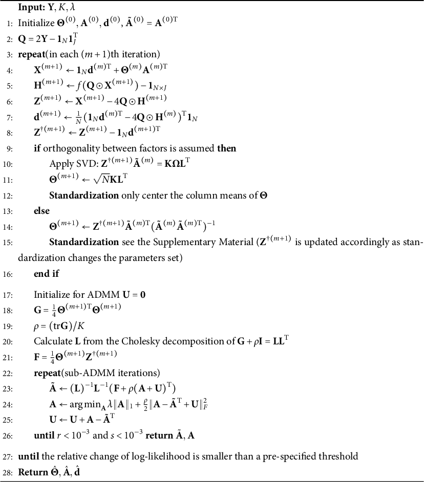
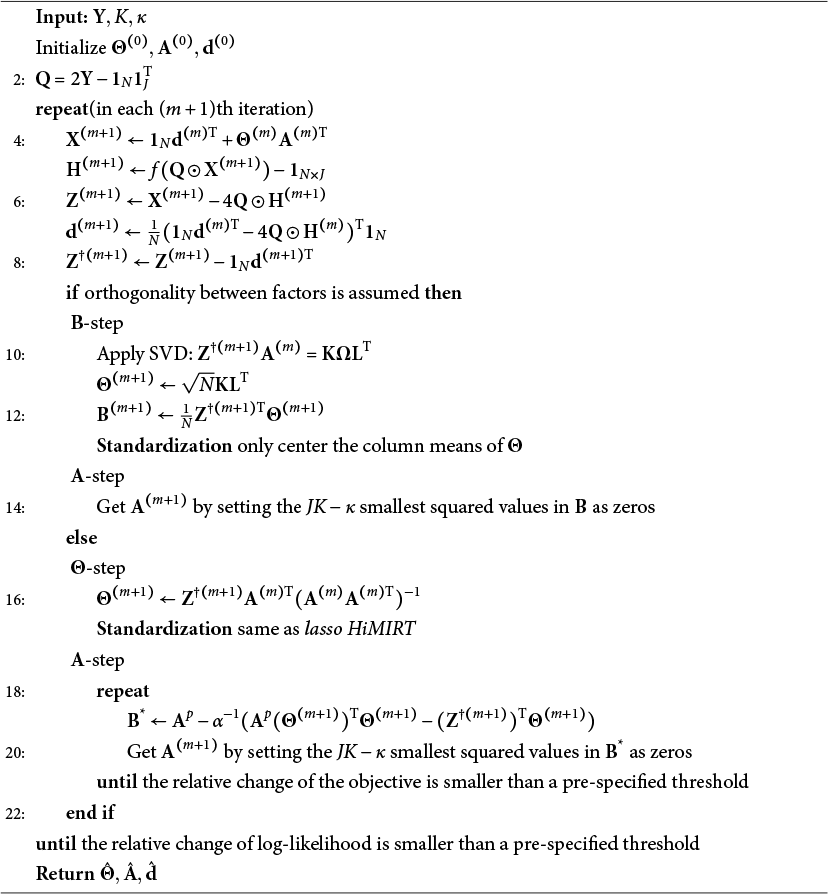
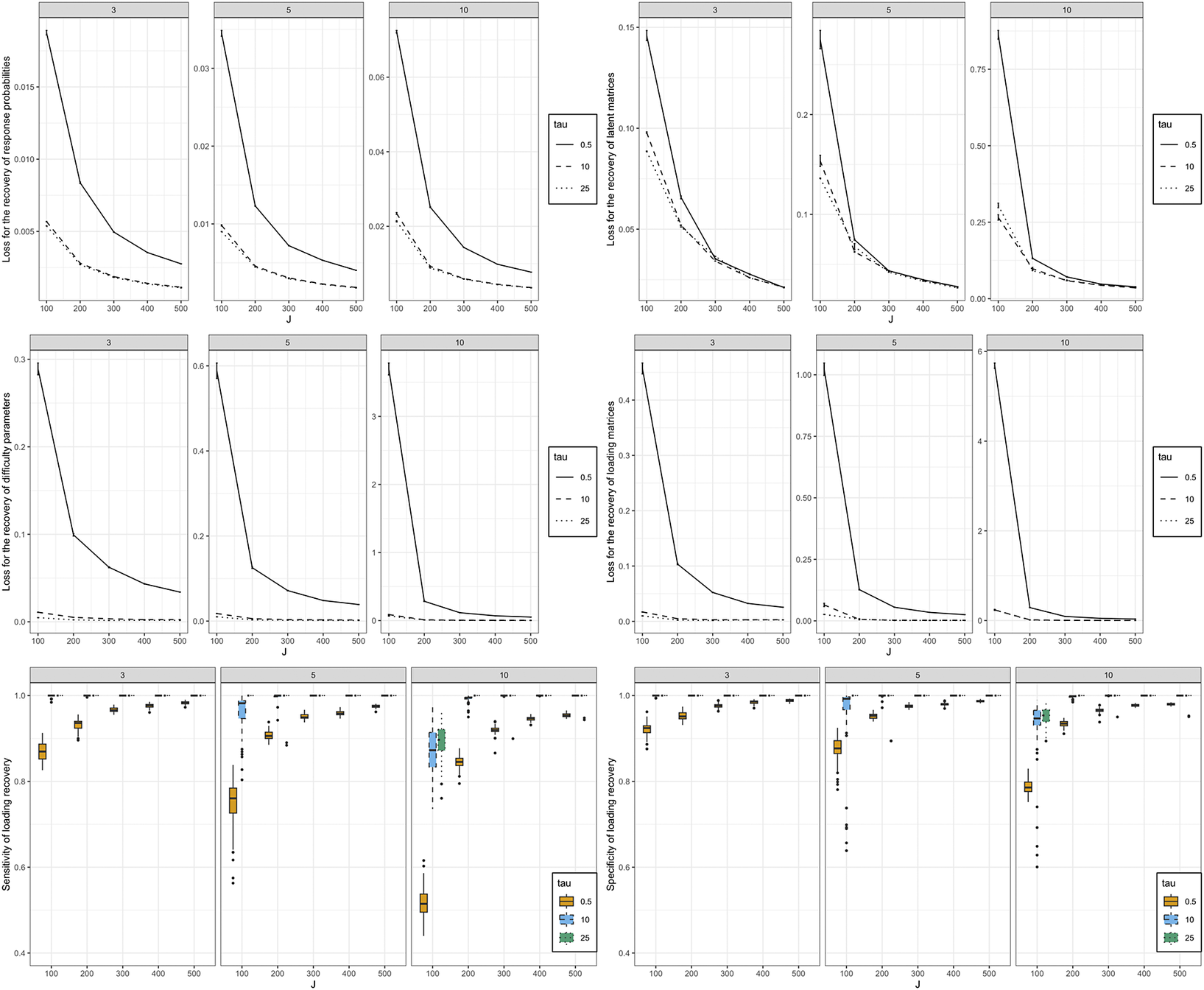
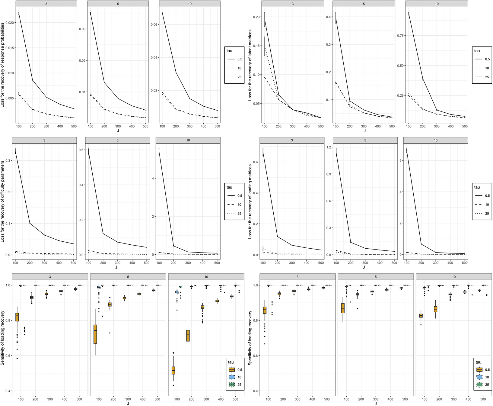
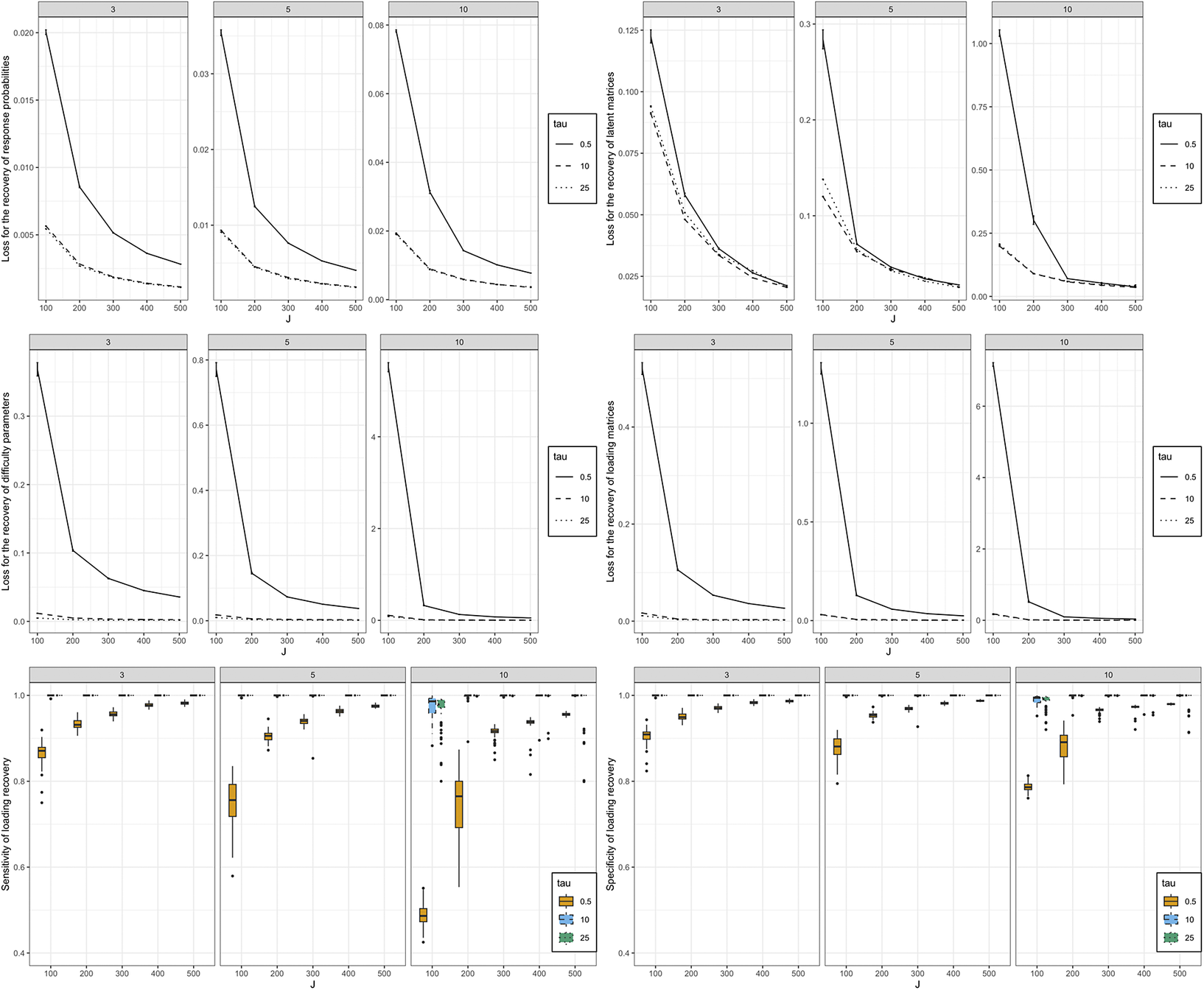
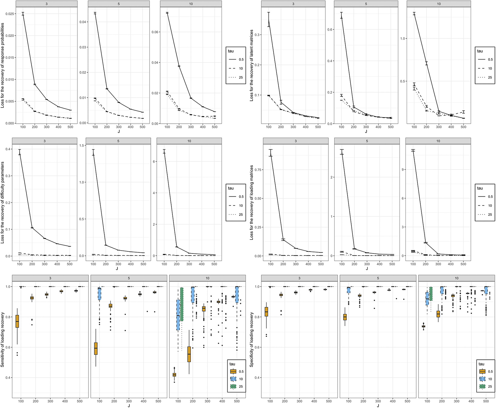
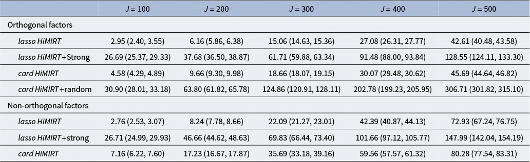
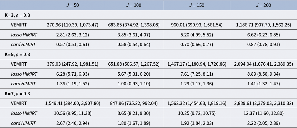

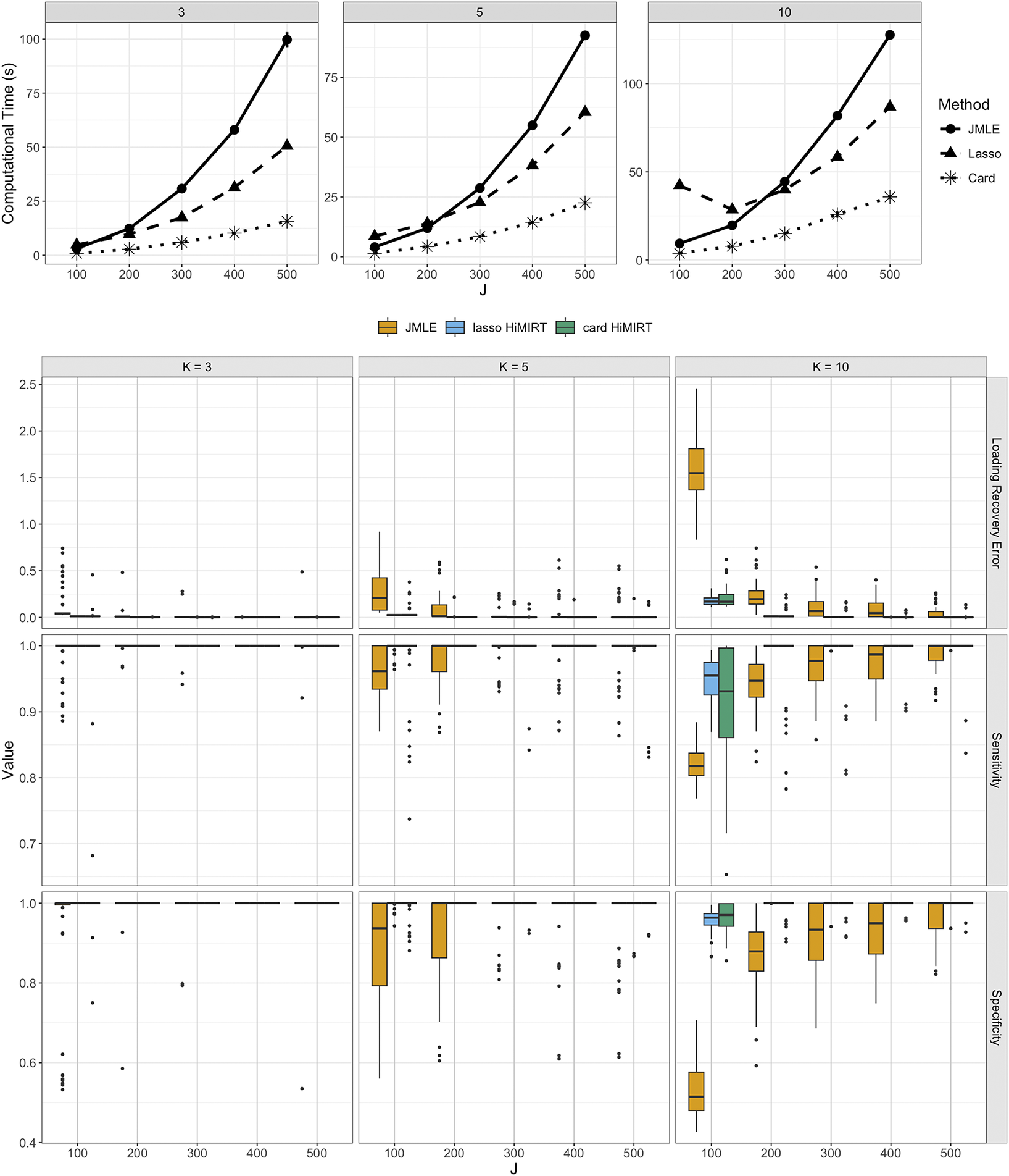
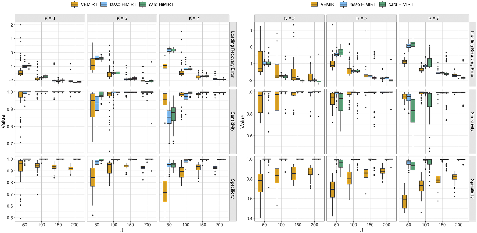


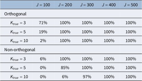

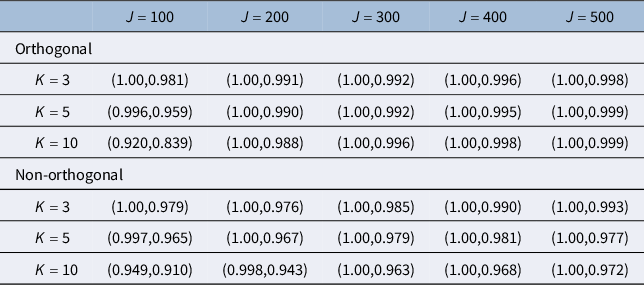
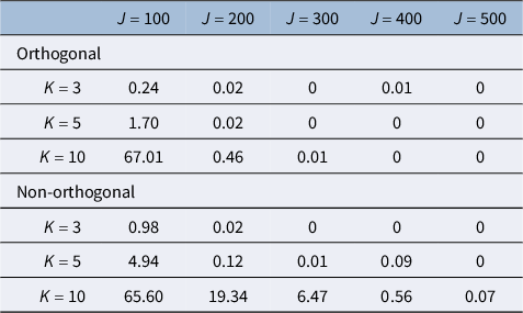
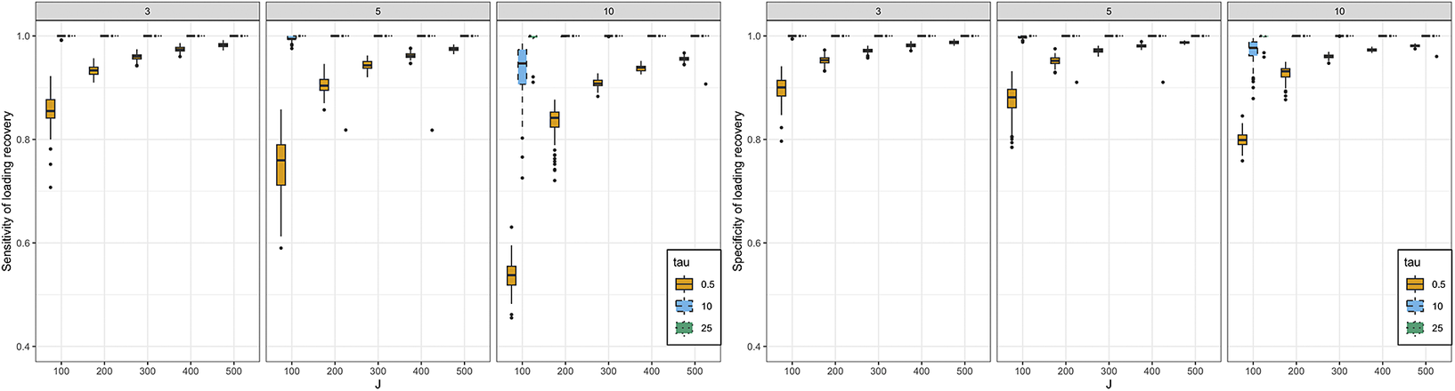
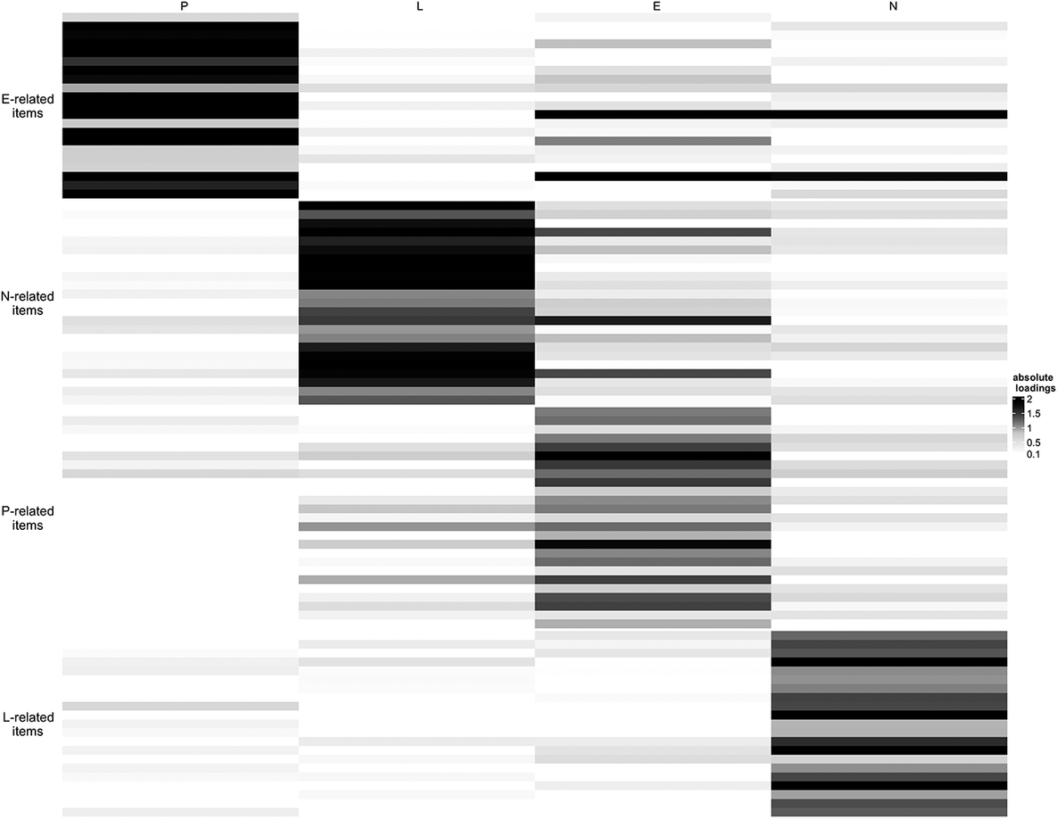
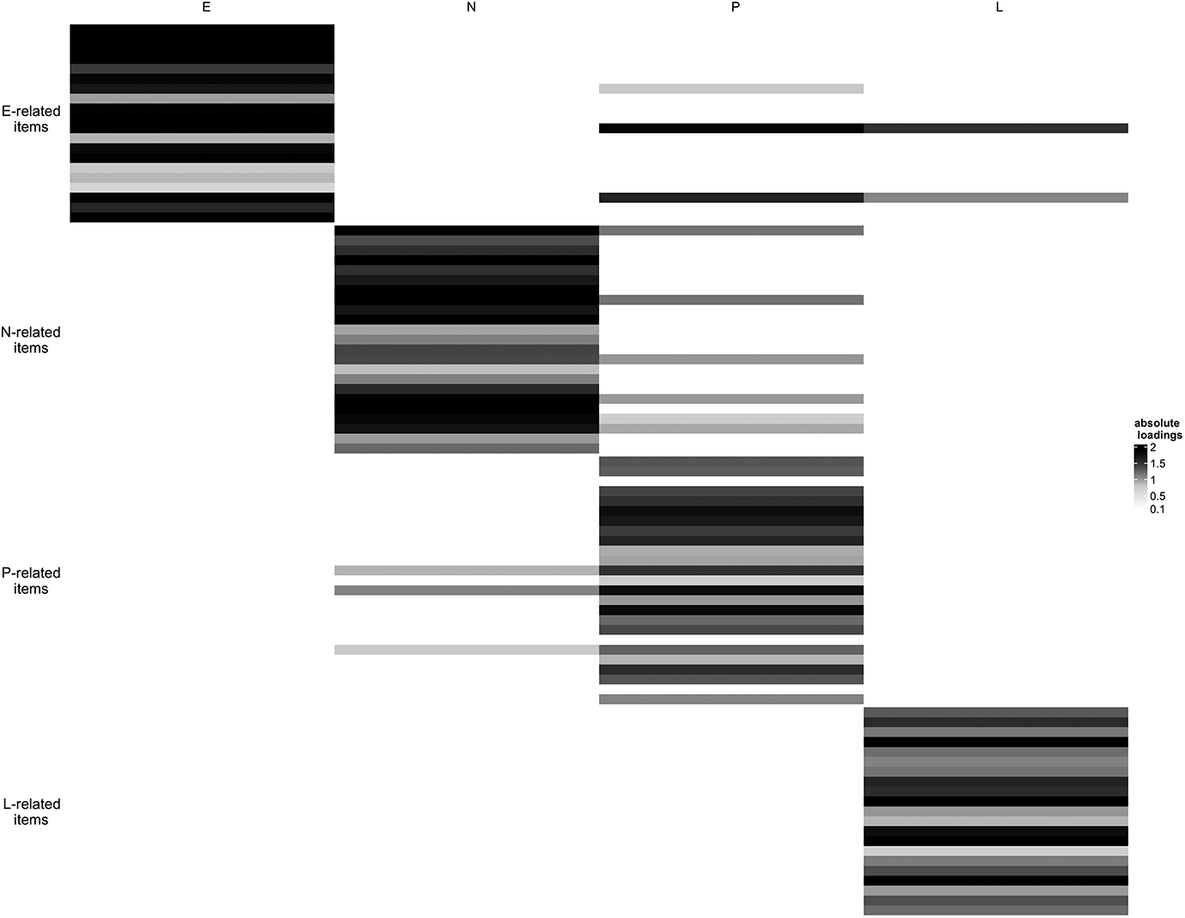
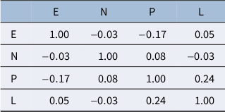
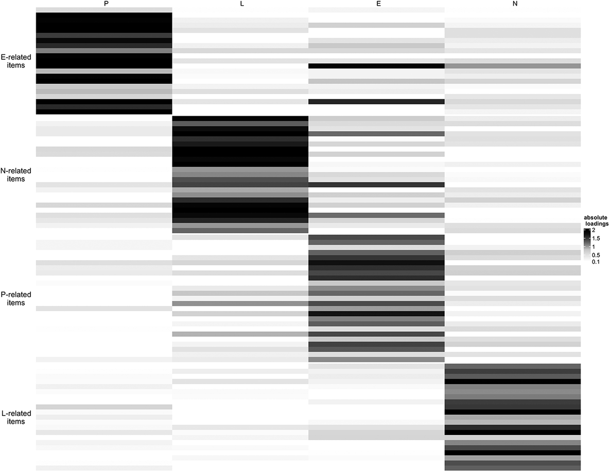
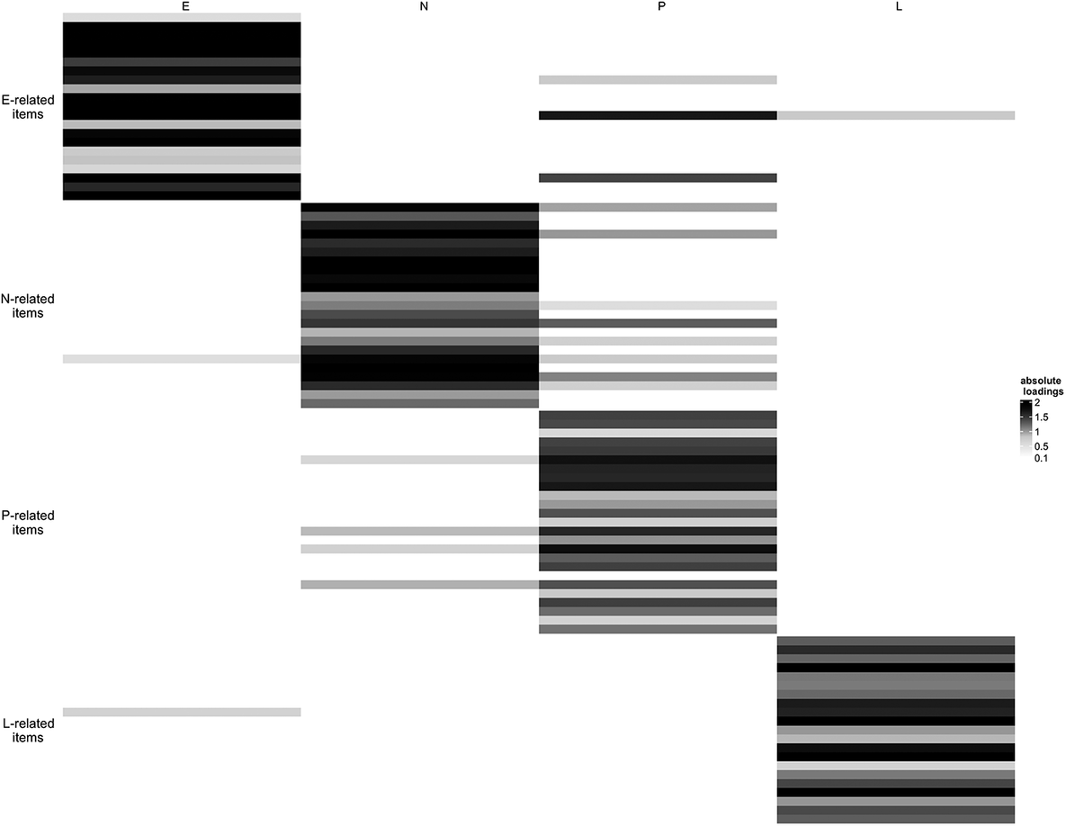



 Open access

