1. Introduction
Global warming exacerbates global economic inequality as poor countries, despite generating fewer greenhouse gas emissions, plunge further into poverty given their increased exposure to the weather and weaker capacity to adapt (Tol et al., Reference Tol, Downing, Kuik and Smith2004; Diffenbaugh and Burke, Reference Diffenbaugh and Burke2019). At the subnational level, where much of the interesting variation in economic activity takes place, however, empirical evidence on the climate-economy relationship remain scarce. Because the poor account for a modest fraction of national income, the detrimental effects of weather shocks on the poor are often obscured using national income accounts. Hence, cross-country level studies providing macroeconomic aggregates are missing the important distributional effects of climate change within countries (Hallegatte and Rozenberg, Reference Hallegatte and Rozenberg2017).
This paper investigates the impact of temperature and precipitation shocks on per capita income growth across municipalities in the Philippines – ranked as the world’s most disaster-prone country by the World Risk Report 2024. Drawing on data from over 1600 municipalities spanning diverse economic profiles and climate zones between 2000 and 2020, we leverage exogenous annual variation in local weather conditions to identify their causal effects on economic growth. We assess the persistence of these impacts over the medium term and explore potential nonlinearities in the response. Additionally, we extend the analysis to the administrative regional level to examine broader spatial dynamics and evaluate the mechanisms through which weather shocks are transmitted.Footnote 1
While an extensive literature based on cross-country level panel data quantifies the adverse effects of weather shocks on economic output,Footnote 2 empirical evidence at the subnational level remains limited. Studies that investigate the climate-economy nexus at the local level include Acevedo et al. (Reference Acevedo, Mrkaic, Novta, Pugacheva and Topalova2020), Kalkuhl and Wenz (Reference Kalkuhl and Wenz2020), Kotz et al. (Reference Kotz, Wenz, Stechemesser, Kalkuhl and Levermann2021), Kotz et al. (Reference Kotz, Levermann and Wenz2022) and Callahan and Mankin (Reference Callahan and Mankin2022). These analyses use a global panel of subnational regions and document robust evidence that temperature and rainfall affect productivity levels locally. Country-specific regional panel studies include Otrachshenko and Popova (Reference Otrachshenko and Popova2022) who look at 79 regions in Russia and reveal that consecutive extremely hot days decrease regional gross domestic product (GDP) per capita, with poor regions suffering more from extreme temperatures than rich regions. Deryugina and Hsiang (Reference Deryugina and Hsiang2014) examine the climate-economy relationship at the county level for 48 states in the US and reveal that extreme temperature days lead to lower productivity and overall economic performance, even in the most advanced economies such as the US.Footnote 3 Burke and Tanutama (Reference Burke and Tanutama2019) look at over 11,000 districts across 37 countries and show that, although country-level estimates are unbiased, they are noisier than district-level estimates and can get the sign of the true relationship wrong. In addition, because cross-country analyses include diverse countries from all over the world, it is often challenging to trace the specific channels through which weather shocks affect the income distribution (Otrachshenko and Popova, Reference Otrachshenko and Popova2022).
An important challenge in identifying the causal links betwen climate and economy relates to the appropriate functional form for the weather variables (Dell et al., Reference Dell, Jones and Olken2014). In most studies, econometric specifications of the climate-economy relationship are often expressed in terms of the growth in GDP per capita and the level of temperature and precipitation. However, Mendelsohn (Reference Mendelsohn2016), Kahn et al. (Reference Kahn, Mohaddes, Ng, Pesaran, Raissi and Yang2021) and Tol (Reference Tol2021) warn that the inclusion of the level of weather variables, since they are trended in almost all countries in the world, introduces a linear trend in income per capita growth which is spurious and not supported by the data, hence resulting in biased estimates. Moreover, except for a few studies such as Kotz et al. (Reference Kotz, Wenz, Stechemesser, Kalkuhl and Levermann2021) and Linsenmeier (Reference Linsenmeier2023, Reference Linsenmeier2024), current panel models do not explicitly model weather variability, an important feature of climate change, in the estimation of damage functions. The relationship between within-year temperature variability and macroeconomic aggregates remains an open question in the literature (Donadelli et al., Reference Donadelli, Jüppner and Vergalli2021).
There is also disagreement over whether the economy-wide effects of weather shocks are temporary only or persistent. If the weather effects are temporary only, that is, the weather affects only the level of output, this level effect eventually reverses itself as the weather returns to its prior state. For example, a negative precipitation shock in a given year, say, drought, may reduce agricultural yields, but once precipitation reverts to its average value, agricultural production bounces back. By contrast, persistent effects of weather shocks imply that they influence not only the level of output but also its growth rate. The growth effect is not reversed (Dell et al. (Reference Dell, Jones and Olken2012), Kalkuhl and Wenz (Reference Kalkuhl and Wenz2020). Droughts may last for extended periods, and a failure to innovate in one period leaves the economy further behind. While Dell et al. (Reference Dell, Jones and Olken2012), Burke et al. (Reference Burke, Hsiang and Miguel2015) and Kahn et al. (Reference Kahn, Mohaddes, Ng, Pesaran, Raissi and Yang2021) establish that temperature shocks affect long-run growth rates especially in poor countries, Acevedo et al. (Reference Acevedo, Mrkaic, Novta, Pugacheva and Topalova2020) and Kalkuhl and Wenz (Reference Kalkuhl and Wenz2020) do not find statistically significant persistent growth effects of warming on GDP. This ‘level-vs.-growth effects’ question is heavily discussed in the literature as empirical findings appear mixed and inconclusive Diffenbaugh and Burke (Reference Diffenbaugh and Burke2019), Rosen (Reference Rosen2019), Kalkuhl and Wenz (Reference Kalkuhl and Wenz2020).
Our paper contributes to this literature in the following ways. First, we examine the climate-economy relationship at the subnational level for the Philippines using the novel nighttime lights (NTL) dataset developed by Chen et al. (Reference Chen, Yu, Yang, Zhou, Yao, Qian, Wang, Wu and Wu2021). To our knowledge, this is the first study that examines the impact of temperature and precipitation shocks on income growth in Philippine municipalities using innovative satellite data. To circumvent the unavailability of timely and reliable subnational income accounts, especially in developing countries, economists have exploited NTL data from satellites, a useful proxy for local economic activity (Henderson et al., Reference Henderson, Storeygard and Weil2012; Keola et al., Reference Keola, Andersson and Hall2015; Gibson et al., Reference Gibson, Olivia, Boe-Gibson and Li2021; Pagaduan, Reference Pagaduan2022). Most economic activities at night require light, thus higher intensity of light implies higher level of economic activity and income, which is increasing in both income per capita and number of people. Calculating growth in NTL per capita at the municipality level, we assess the disproportional and heterogeneous within-country effects of weather shocks on income growth across the level of economic development.
Second, in addition to the average temperature and precipitation levels, we use two other functional forms of weather shocks, namely, deviations of temperature and precipitation from their respective long-run (i.e., 20-year) moving average historical norm following Kahn et al. (Reference Kahn, Mohaddes, Ng, Pesaran, Raissi and Yang2021),Footnote 4 and within-year variability of temperature and precipitation as measured by the standard deviation following Donadelli et al. (Reference Donadelli, Jüppner and Vergalli2021). On the one hand, measuring weather shocks in terms of deviations from their historical norm and within-year variability alleviates concerns about the econometric pitfalls of using trended variables such as levels in growth regressions. On the other, this allows us to evaluate the differential effects of weather across several dimensions of climate change.
Third, we contribute to the level-vs.-growth debate by explicitly testing for the persistence of the effects of weather shocks using distributed lag models following Dell et al. (Reference Dell, Jones and Olken2012). We also test for the presence of nonlinear effects, an important result in the dominant climate-economy literature. We then estimate the effects of the weather at the regional level and examine the specific transmission channels using sector-disaggregated administrative region-level income accounts. Our analysis offers a granular perspective to the persistent effects of temperature and precipitation shocks and the mechanisms that allow for the propagation of their effects on growth.
Our study reveals important insights. First, temperature variability dampens growth, but only in poor municipalities. A 1∘C increase in the annual standard deviation in temperature reduces growth by 0.20 percentage points (pp) in poor municipalities. Second, poor municipalities suffer the largest costs of temperature variability in the medium run. In the distributed lag models, the cumulative effect of increased temperature volatility in poor municipalities remains substantially negative as more lags are included. These dynamics reflect the persistent negative effects of increased temperature variability on poor municipalities due to weak adaptive capacity and greater vulnerability to weather anomalies. Third, we identify nonlinear responses to weather shocks. An additional day exceeding  $25.1^\circ\,\mathrm{C}$ reduces growth by 0.01 pp, while one more day with temperature below
 $18.5^\circ\,\mathrm{C}$ increases growth by 0.02 pp. These nonlinear effects are robust across various specifications and sensitivity checks. Finally, we extend our analysis to the regional level to examine the transmission mechanisms of weather shocks. Temperature and precipitation anomalies primarily affect income growth through reductions in agricultural productivity and service sector performance – particularly in wholesale and retail trade, health and education. At the regional level, a
 $1^\circ\,\mathrm{C}$ increase in temperature variability reduces agricultural growth by 6.4 pp, while deviations in average temperature suppress service sector growth by 3.5–4.4 pp. Precipitation shocks exert milder but still notable effects, lowering agricultural and service growth by approximately 1 and 0.5 pps, respectively. No statistically significant impacts are observed in industrial sectors. Overall, our findings highlight the importance of understanding the distributional effects of climate change within countries, its underlying mechanisms, and how economic development policies can help shield poor municipalities from the vagaries of the weather.
The rest of this paper is organized as follows. Section 2 presents the data sources and empirical strategy.Footnote 5 Section 3 discusses the results and robustness checks, while the last section concludes.
2. Data and methodology
2.1. Data sources
To construct our dataset, we combine the novel NTL dataset of Chen et al. (Reference Chen, Yu, Yang, Zhou, Yao, Qian, Wang, Wu and Wu2021) with the high-resolution AgERA5 data based on the ERA5 reanalysis produced by the European Centre for Medium-Range Weather Forecasts (ECMWF). For the regional analysis and transmission channels, we use official income accounts from the Regional Accounts of the Philippines provided by the Philippine Statistics Authority (PSA). Gridded population data are drawn from the Gridded Population of the World (GPW) version 4 product of the Center for International Earth Science Network at Columbia University. Lastly, we obtain administrative boundaries shapefiles from the Database of Global Administrative Areas (GADM).
Chen et al. (Reference Chen, Yu, Yang, Zhou, Yao, Qian, Wang, Wu and Wu2021) produce an extended annual time series of the Suomi National Polar-orbiting Partnership Visible Infrared Imaging Radiometer Suite (NPP-VIIRS) NTL data, covering the period 2000–2020.Footnote 6 To construct a proxy for growth in income per capita at the municipality level, we aggregate the light intensities at the GADM level 2 administrative boundaries using ArcGIS version 10.7.1, a geographic information system software, and normalize it by the gridded population count at the same level. Then, we calculate the growth rate as the year-on-year change in the logarithm of NTL per capita. This results in a rich dataset of municipality-level growth in NTL per capita consisting of 32,560 municipality-year observations over the period 2001–2020.
For our weather data, we use AgERA5 which provides daily surface meteorological data from 1979 to the present designed for agriculture and agro-ecological studies. This dataset is derived from the ERA5 data, the fifth generation ECMWF reanalysis for the global climate and weather.Footnote 7 We exploit the daily average temperature (∘C) and the daily average precipitation (mm) series from 1979–2020 to construct annualized measures of weather anomalies.Footnote 8 To identify the causal effects of weather shocks, we exploit the random annual variations in three different functional forms of the weather variables. First, we use the average annual temperature and precipitation levels, calculated as the simple average of daily temperature and precipitation for each year, respectively. Schlenker and Roberts (2009) and Deschênes and Greenstone (Reference Deschênes and Greenstone2007) pioneered the use of this approach, and several authors in the climate-economy literature – including Dell et al. (Reference Dell, Jones and Olken2012), Lanzafame (Reference Lanzafame2014), Burke et al. (Reference Burke, Hsiang and Miguel2015), Acevedo et al. (Reference Acevedo, Mrkaic, Novta, Pugacheva and Topalova2020) and Kalkuhl and Wenz (Reference Kalkuhl and Wenz2020) – have followed suit. Our second measure uses the deviation of average annual temperature and precipitation from their respective long-term (i.e., 20-year) moving average historical norm following Kahn et al. (Reference Kahn, Mohaddes, Ng, Pesaran, Raissi and Yang2021). Finally, we explicitly model weather variability, an important feature of climate change, by using the annual standard deviation of daily temperature and precipitation as our third functional form for the weather shocks following Donadelli et al. (Reference Donadelli, Jüppner and Vergalli2021).
Finally, we obtain the data on the real growth in gross regional domestic product (GRDP) for each of the 17 administrative regions in the Philippines, as well as the real growth in the gross value added (GVA) of each of the three main sectors (agriculture, industry and services) and 15 subsectors from the PSA. The 2020 Regional Accounts of the Philippines provides annual information on GRDP by administrative region from 2000–2020 at constant 2018 prices.
2.2. Methodology
We run panel regressions of the form
 \begin{equation}
Y_{it} = \phi_i + \theta_{t} + \sum_{j=0}^{L}\rho_j^TT_{i,t-j} + \sum_{j=0}^{L}\rho_j^RR_{i,t-j} + \varepsilon_{it},
\end{equation}
where Yit denotes the year-on-year change in the logarithm of NTL per capita in municipality i at year t, ϕi are municipality fixed effects, θt are year fixed effects, Tit and Rit a vector of annual temperature and precipitation shocks with up to lags L included, respectively, and ɛit is an idiosyncratic error term. Weather shocks are often correlated across small scales of aggregation. Municipalities may suffer from a weather shock simply because their neighbouring municipalities are also affected. That is, spatial dependence may exist and drive the results. We address this concern by (i) using robust standard errors clustered at the province level and (ii) employing Driscoll and Kraay (Reference Driscoll and Kraay1998) standard errors which allow for spatial dependence at arbitrary scales. Our fixed effects structure is parsimonious in that we control for municipality fixed effects and year fixed effects. Alternatively, one could also control for province by year fixed effects. However, as shown by Fisher et al. (Reference Fisher, Hanemann, Roberts and Schlenker2012), Li et al. (Reference Li, Cong, Gu and Zhang2021) and Deryugina and Hsiang (Reference Deryugina and Hsiang2014), controlling for province-year fixed effects removes most of the signal since much of the identifying variation in the weather occurs at the province level. We estimate variations of equation (1) where we interact the weather shocks with “poor” dummy variable to test the disproportional and heterogeneous effects of weather shocks across the level of economic development. In our baseline specifications, a municipality is defined as “poor” when its poverty incidence in the year 2000, as taken from the small-area estimates of poverty by NSCB (2005), is above the third quartile of the distribution.Footnote 9 In our robustness checks in the online appendix, we test whether our results are sensitive to outliers and alternative definition of “poor”.
Because temperature and precipitation shocks vary exogenously over time as random draws from the distribution of weather in a given spatial area, the weather-shock approach in equation (1) offers strong identification properties. Municipality fixed effects, ϕi, absorb fixed spatial characteristics, both observed and unobserved, hence disentangling the shocks from various possible sources of omitted variable bias. Year fixed effects, θt, further purge common trends to ensure that the climate-economy relationship is strongly identified from idiosyncratic local shocks. Equation (1) uses a reduced-form panel approach that makes relatively few identification assumptions but allows unusually strong causative interpretation.Footnote 10
We estimate equation (1) with no lags and test the null hypothesis that temperature and precipitation shocks do not affect growth:  $ H_0 (L=0):\rho_0 = 0 $. A failure to reject this hypothesis implies that weather shocks do not affect growth in both the short and the medium terms, that is, there are no level and growth effects. Then, we estimate separately the model that includes one through five lags. Under each lag length specification, we test separately the immediate effect of weather shocks,
 $ H_0^1 (L \gt 0):\rho_0=0 $, and their cumulative effects,
 $ H_0^2 (L \gt 0):\sum_{j=0}^L\rho_j =0 $. A failure to reject the hypothesis that the cumulative effect is equal to zero indicates that the effects of weather shocks do not persist in the medium run, that is, there is no growth effect.
3. Results
3.1. Baseline results
3.1.1. Level effect
We estimate equation (1) with no lags and test the null hypothesis that weather shocks do not affect growth:  $ H_0 (L=0):\rho_0 = 0 $. Table 1 presents the baseline results and shows the effects of temperature and precipitation shocks on the growth rate of municipality-level NTL per capita using the full sample of 1628 localities in the period 2001–2020. The regression in columns 1 and 2 uses the average level of shocks, in columns 3 and 4 the deviation from moving average, and in columns 5 and 6 the standard deviations. Columns 1, 3 and 5 show a negative but statistically insignificant relationship between temperature fluctuations and growth across all municipalities. In the same columns, the coefficients of the precipitation shocks are also statistically insignificant, except for the standard deviation of precipitation which is positive and statistically significant.
Baseline results

Notes: The dependent variable for all columns is the growth rate of municipality-level nighttime lights (NTL) per capita. All columns include municipality fixed effects and year fixed effects. Robust standard errors adjusted for clustering at the province level are in parentheses, while Driscoll and Kraay (Reference Driscoll and Kraay1998) standard errors which allow for spatial dependence at arbitrary scales are in brackets. Poor municipality is a dummy variable for municipalities with poverty incidence above the third quartile in the year 2000 as taken from the small-area estimates of poverty by NSCB (2005). Average temperature is in  $^\circ\mathrm{C}$, while average precipitation is in mm per year. Deviation from moving average (Dev from MA) refers to the deviations from their respective 20-year moving average historical norm. Standard deviation measures within-year variability.
At the national level, evidence on the ability of economic development to help countries cope with weather shocks and reduce the damages they cause appears ambiguous. In advanced economies, most people live in durable housing conducive to withstanding extreme weather conditions with attributes such as good thermal insulation and air-conditioning (Barreca et al., Reference Barreca, Clay, Deschênes, Greenstone and Shapiro2016), high-quality roofs and strong foundations. Also, institutional factors such as better government policies help them combat the adverse effects of the weather (Acevedo et al., Reference Acevedo, Baccianti, Mrkaic, Novta, Pugacheva and Topalova2019; Acevedo et al., Reference Acevedo, Mrkaic, Novta, Pugacheva and Topalova2020). Yet a host of micro-level evidence suggests that warming could substantially reduce economic production, even in highly developed countries, through several mechanisms such as depressed labour and total factor productivity (Zhang et al., Reference Zhang, Deschênes, Meng and Zhang2018), poorer cognitive function (Heyes and Saberian, 2018), and worse health conditions (Burke et al., Reference Burke, González, Baylis, Heft-Neal, Baysan, Basu and Hsiang2018).
To test whether economic development plays a role, in columns 2, 4 and 6 of table 1, we interact the weather shocks with a dummy variable for a “poor” municipality, defined as having poverty incidence above the third quartile of the distribution in the year 2000 as taken from the small-area estimates of poverty by NSCB (2005). The coefficients on the interaction between the “poor” dummy and temperature shocks are all negative, but only the standard deviation of temperature (column 6) is statistically significant. The coefficients on the interaction between the “poor” dummy and precipitation shocks are all positive and statistically significant. In the bottom portion of table 1, we report the overall effect of the weather shocks on growth in poor municipalities. A 1  $^\circ\mathrm{C}$ increase in the standard deviation of temperature decreases growth by 0.2 pp, but only in poor municipalities (column 6). On the other hand, a 1 mm increase in precipitation, either in terms of level (column 2), deviation from moving average (column 4), or standard deviation (column 6), results in a small increase of 0.02–0.05 pp in growth in poor municipalities. Therefore, we reject the null hypothesis that weather fluctuations have no level (instantaneous) effect on growth in poor municipalities. In poor municipalities, higher variability in temperature dampens growth considerably, although increased precipitation slightly raises growth in the same municipalities. This result highlights the heterogeneous effects of the weather across both the level of economic development of municipalities and the nature of weather shocks.
Table A2 in the online appendix reports the baseline results when outliers are removed from the sample. To avoid the potential unfavourable effect of outliers, we truncate the growth rate of the municipality-level NTL per capita variable before estimating equation (1) by dropping the NTL observations above 99 per cent and below 1 per cent of the distribution. The level effect of increased temperature variability on poor municipalities is robust to the potential impact of outliers, although the estimated impact becomes smaller in magnitude when outliers are excluded. The decrease in growth in poor municipalities from a  $1^\circ\,\mathrm{C}$ increase in the standard deviation of temperature becomes milder at 0.1 pp but still statistically significant. The positive effect of more precipitation in all three functional forms, however, further weakens and becomes closer to zero. In fact, the positive impact of higher deviation of precipitation from the moving average in column 4 is no longer statistically significant. In table A3, we present the baseline results under an alternative definition of a “poor” municipality. Under this definition, a “poor” municipality is one with poverty incidence above the median in the year 2000 as taken from the small-area estimates of poverty by NSCB (2005). The level effect of more volatile temperature remains consistent under this alternative definition of “poor”, although, as in table A2, the estimated impact for poor municipalities becomes smaller in magnitude and slightly less statistically significant. The positive effect of more precipitation becomes weaker. Given these robustness checks, we conclude that the substantially negative effect of increased temperature volatility on growth in poor municipalities is robust, while the small positive effect of increased rainfall seems to further weaken under alternative checks.
Our finding that increased temperature variability hurts economic growth is aligned with existing studies in the literature. Kotz et al. (Reference Kotz, Wenz, Stechemesser, Kalkuhl and Levermann2021) find that an extra degree Celsius of day-to-day variability in a given year reduces regional growth rates by at least five percentage points. Linsenmeier (Reference Linsenmeier2023) reveals that one sample standard deviation of day-to-day variability ( $1.44^\circ\,\mathrm{C}$) and seasonal (intra-annual) variability (
 $14.71^\circ\,\mathrm{C}$) reduces nightlights by 16 and 9 per cent, respectively. It is unlikely that increased agricultural production from more rainfall characterizes the weakly positive effect of precipitation that we find in table 1. First, we use NTL in our analysis, a strong proxy for economic growth in industry and services sectors but a weak indicator for growth in the agricultural sector in the Philippines (Pagaduan, Reference Pagaduan2022). A more plausible explanation is that, after a natural disaster from heavy rainfall such as flooding, basic infrastructures in affected municipalities are back on line first, so one could imagine that NTL recovers faster than GDP or income. Second, as we show in section 3.1.4, this small positive effect of rainfall on NTL is rather short-lived, that is, we find no strong evidence of its cumulative effect in the medium run. Finally, in section 3.3 in our regional analysis, we show that extreme rainfall can in fact dampen growth at the regional level through dampened agricultural activity and disrupted activities in services sectors such as wholesale and retail trade, health and education.
The result that weather shocks disproportionately affect growth in poor municipalities is consistent with previous studies that reveal the unequal impact of weather shocks on growth. Acevedo et al. (Reference Acevedo, Mrkaic, Novta, Pugacheva and Topalova2020) show that a  $1^\circ\,\mathrm{C}$ increase in temperature in a given year reduces growth by 1.1 pp for regions in low-income developing countries; this impact is three times more sizable than the marginal effect on regions in advanced economies. Kalkuhl and Wenz (Reference Kalkuhl and Wenz2020) find that a similar shock in a poor and hot region (temperature of
 $25^\circ\,\mathrm{C}$) decreases output by 3 per cent while there are no statistically significant effects for rich and colder regions (temperature of
 $10^\circ\,\mathrm{C}$). Kotz et al. (Reference Kotz, Wenz, Stechemesser, Kalkuhl and Levermann2021) reveal that lower-income regions are the most vulnerable to changes in day-to-day temperature variability because of more limited resources, as well as their location, as lower-income regions usually reside in lower latitude and coastal areas. Callahan and Mankin (2022) find that warm tropical regions with lower incomes suffer the most from extreme temperatures. At the national level, Dell et al. (Reference Dell, Jones and Olken2012) document that the net effect of a
 $1^\circ\mathrm{C}$ rise in annual temperature is a growth decline of 1.4 pp in poor countries while there is no statistically significant impact on the rich ones. More generally, existing evidence suggests that the poor suffer the brunt of warming because they are more vulnerable to a given increase in temperature, perhaps because they are more exposed to climate-sensitive industries such as agriculture, or because they lack resources such as savings that tend to mitigate the negative effects of weather shocks (Hallegatte et al., Reference Hallegatte, Bangalore, Bonzanigo, Fay, Kane, Narloch, Rozenberg, Treguer and Vogt-Schilb2016; Hallegatte and Rozenberg, Reference Hallegatte and Rozenberg2017; Burke and Tanutama, Reference Burke and Tanutama2019; Hsiang et al., Reference Hsiang, Oliva and Walker2019). On the other hand, the negative effects of the weather are smaller in higher-income countries with well-developed financial sectors which provide better insurance and risk-management policies.
3.1.2. Cumulative effect
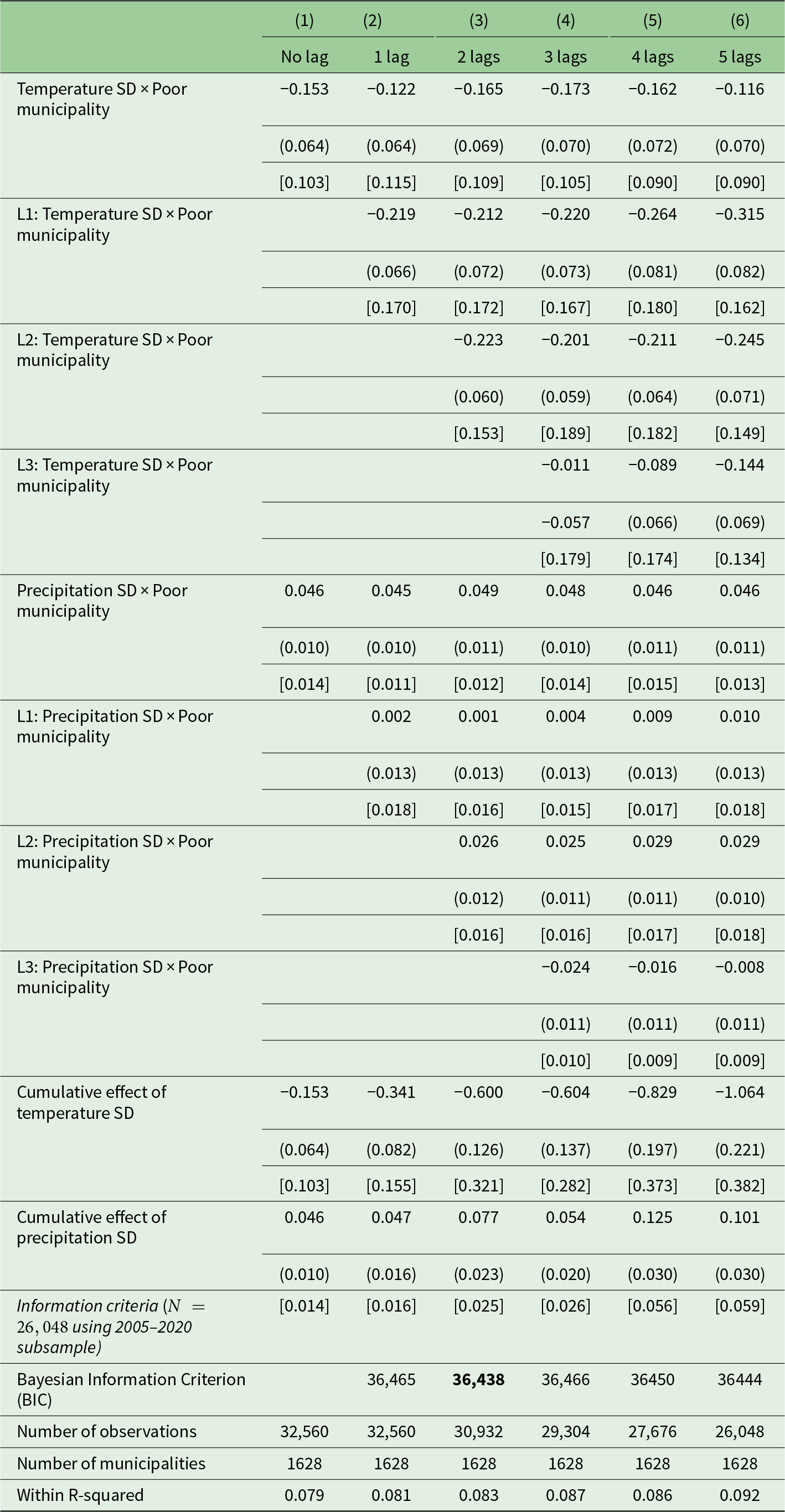
The results above, using the baseline specification with no lags, reject the null hypothesis that the standard deviation of temperature and the level, deviation from moving average, and standard deviation of precipitation have no effect on growth in poor municipalities. Are these level effects likely to persist in the medium run (i.e., growth effects)? Conversely, do the poor catch up after a temporary shock in temperature and precipitation (i.e., level effects)? This section estimates the panel-distributed lag models in equation (1) with up to five lags of the weather variables to explore the dynamics of the weather effects on growth in poor municipalities. The distributed lag models capture both the level (instantaneous) effect and the growth (cumulative) effect. Table 2 and tables A4–A11 report the estimates from the distributed lag models. In all these tables, we show the coefficients of the lagged weather variables as well as the cumulative effect of the weather shock, which is calculated as the sum of coefficients of all lagged weather variables. To determine the most optimal lag specification, we use two approaches. The first method is through statistical significance where we start first with lag 0 and proceed successively with the subsequent lags. This method requires that the subsequent lag must be statistically significant. The second method involves the use of the Bayesian information criterion (BIC). The most optimal lag specification is one which minimizes the BIC.
Standard deviation (SD) of weather shocks with lags

Notes: The dependent variable for all columns is the growth rate of municipality-level NTL per capita. All columns include municipality fixed effects and year fixed effects. Robust standard errors adjusted for clustering at the province level are in parentheses, while Driscoll and Kraay (Reference Driscoll and Kraay1998) standard errors which allow for spatial dependence at arbitrary scales are in brackets. Poor municipality is a dummy variable for municipalities with poverty incidence above the third quartile in the year 2000 as taken from the small-area estimates of poverty by NSCB (2005). Given space constraints, the table only reports the coefficients for lags 0–3 of the weather shocks. The cumulative effect is the sum of coefficients of all lagged weather variables. Standard deviation (SD) measures within-year variability.
Table 2 shows the dynamic effects of temperature and precipitation variability. For temperature, columns 1–6 show that the coefficients are consistently negative and statistically significant up to lag 2 of the temperature shock. Column 6 shows that even the coefficient of lag 3 is still negative and statistically significant. This suggests that the negative effect of increased temperature variability persists for at least two years after the initial shock. For precipitation, on the other hand, while all the columns show that the instantaneous effect, the coefficient of lag 0, is consistently positive and statistically significant, the coefficient of lag 1 becomes consistently statistically insignificant. The model with two lags of the weather shocks in column 3 minimizes the BIC. Hence, the cumulative effect of increased temperature volatility in poor municipalities remains substantially negative as more lags are included.
In tables A4 and A5, we test whether this cumulative effect is robust to outliers and alternative definition of “poor”, respectively. The cumulative negative effect of temperature variability remains consistent, while the lag coefficients of precipitation lose their statistical significance. The adverse effects of increased temperature volatility on the poor persist, rather than reverse, in the medium run. On the other hand, the small positive effect of increased precipitation volatility is rather short-lived.Footnote 11
We find that the the adverse effects of increased temperature volatility on the poor persist, rather than reverse, in the medium run. On the other hand, the weak benefits of more precipitation, either in terms of the level, deviation from moving average, or standard deviation, tend to be more short-lived in poor municipalities. Our results are consistent with the findings of Kotz et al. (Reference Kotz, Levermann and Wenz2022), which show that the negative effects of day-to-day variability in temperature persist for at least two years following the initial shock. Dell et al. (Reference Dell, Jones and Olken2012) and Burke et al. (Reference Burke, Hsiang and Miguel2015) also find persistent negative effects of temperature on poor countries, confirming the presence of growth effects. Li et al. (Reference Li, Cong and Gu2020), studying counties in China, reveal that the magnitude of temperature’s cumulative effect increases as more lagged variables are included in the model. On the other hand, the cumulative effect of precipitation only shows up in the medium run, that is, only when 5 lags or 10 lags are included in the model.
3.2. Nonlinear effects of weather shocks
Several empirical studies such as Burke et al. (Reference Burke, Hsiang and Miguel2015), Zhang et al. (Reference Zhang, Deschênes, Meng and Zhang2018), Burke and Tanutama (Reference Burke and Tanutama2019), Li et al. (Reference Li, Cong and Gu2020), Li et al. (Reference Li, Cong, Gu and Zhang2021) and Otrachshenko and Popova (Reference Otrachshenko and Popova2022) reveal that temperature and rainfall shocks affect economic productivity in a nonlinear fashion. In this section, we test for the presence of nonlinear effects of weather shocks on growth. We construct weather bins according to the distribution of weather realizations in our sample. Based on this observed distribution, we construct a fixed number of equal-width bins for both temperature and precipitation and count the number of days in a given year for which each municipality’s weather falls within that particular bin. Figure A3 in the online appendix shows the distribution of our weather variables. We estimate the following empirical specification:
 \begin{equation}
Y_{it} = \phi_i + \theta_{t} + \sum_{n=1}^{N}\alpha^n{T\_bin}_{i,t}^n + \sum_{m=1}^{M}\beta^m{R\_bin}_{i,t}^m + \varepsilon_{it},
\end{equation}
where Yit denotes the year-on-year change in the logarithm of NTL per capita in municipality i at year t, ϕi are municipality fixed effects, and θt are year fixed effects. 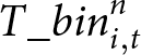 $ {T\_bin}_{i,t}^n $ and
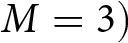
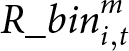 $ {R\_bin}_{i,t}^m $ denote the number of days in municipality i in a given year t that the average temperature and precipitation fall in the nth and mth bin, respectively. In our main specification, we construct N = 5 and M = 5 temperature and precipitation bins. The first temperature level bin is
 $ \lt 18.5^\circ C$ and measures the number of days in municipality i and year t that the average temperature is below
 $18.5^\circ\,\mathrm{C}$. The first precipitation level bin is
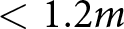 $ \lt 1.2m$ and counts the number of days in municipality i and year t that the average precipitation is below 1.2 m. The bins for the deviation of weather from moving average and the standard deviation of weather are calculated and interpreted in a similar fashion. For both temperature and precipitation, we choose the third bin as the reference bin. Hence, the coefficients α n and β m measure the marginal effect of an additional day in the nth and mth temperature and precipitation bin on growth relative to a day with average temperature and precipitation in the reference bin, respectively. In our robustness checks, we use alternative reference bins and bin widths.
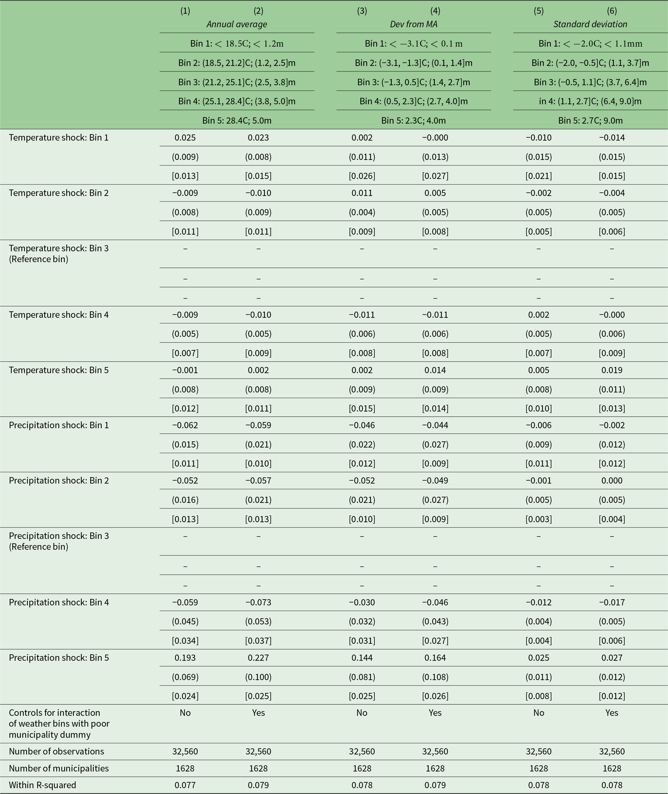
Table 3 presents the nonlinear effects of weather shocks on growth. Columns 1, 3 and 5 present the estimates from the main specification in equation (2), while in columns 2, 4 and 6, we interact each of the weather bins with the ‘poor” dummy variable to examine possible heterogeneous nonlinear effects. We find that the effects of temperature and precipitation shocks on growth across all municipalities are nonlinear. Columns 1 and 2 show that relative to a reference day with an average temperature in  $ (21.2, 25.1]^\circ C$, a day hotter than 25.1
 $^\circ C$ reduces growth by 0.01 pp, while an extra day below
 $18.5^\circ\,\mathrm{C}$ raises growth by 0.02 pp. Relative to a reference day with an average precipitation in
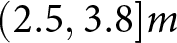 $ (2.5, 3.8]m$, a day with more precipitation than 3.8 m raises growth significantly by at least 0.2 pp, while a day below it decreases economic activity by at least 0.05 pp. In terms of deviation from moving average in columns 3 and 4, a day hotter by
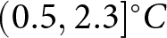 $ (0.5, 2.3]^\circ C $ than its historical norm relative to the reference bin decreases growth by at least 0.01 pp. A day with higher precipitation of more than 4.0 m than its historical norm increases growth by at least 0.14 pp, while anything below this deviation decreases growth by at least 0.05 pp. In columns 5 and 6, we do not find nonlinear effects of temperature variability, while a day with precipitation variability of more than 9.0 m increases growth by at least 0.02 pp and a day with precipitation variability in
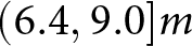 $(6.4, 9.0]m$ decreases growth by at least 0.01 pp.Footnote 12
Nonlinear effects of weather shocks

Notes: The dependent variable for all columns is the growth rate of municipality-level NTL per capita. All columns include municipality fixed effects and year fixed effects. Robust standard errors adjusted for clustering at the province level are in parentheses, while Driscoll and Kraay (Reference Driscoll and Kraay1998) standard errors which allow for spatial dependence at arbitrary scales are in brackets. Poor municipality is a dummy variable for municipalities with poverty incidence above the third quartile in the year 2000 as taken from the small-area estimates of poverty by NSCB (2005). Average temperature is in  $^\circ\mathrm{C}$, while average precipitation is in mm per year. Deviation from moving average (Dev from MA) refers to the deviations from their respective 20-year moving average historical norm. Standard deviation measures within-year variability.
Our results on the nonlinear effects of weather shocks on growth are broadly consistent with existing studies. Li et al. (Reference Li, Cong, Gu and Zhang2021) examine the nonlinear effects of average temperature and precipitation on growth in Chinese counties and find that a day hotter than  $20^\circ\,\mathrm{C}$ has significant negative effects on county-level GDP. The adverse effects of hot days intensify as the temperature increases. They also find that a day with moderate precipitation of
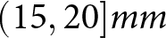 $(15, 20]mm$ positively affects county-level GDP, although this result is not stable in some robustness checks. Otrachshenko and Popova (Reference Otrachshenko and Popova2022) look at the nonlinear effects of weather on Russian regions’ economic growth and find that each consecutive hot day (above
 $25^\circ\,\mathrm{C}$) reduces GDP per capita by 0.19 per cent relative to a single day with the temperature falling in
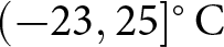 $(-23, 25]^\circ\,\mathrm{C}$. They further find that single hot days do not affect GDP. They do not find statistically significant nonlinear effects of precipitation on GDP per capita.
3.3. Regional analysis and transmission channels
3.3.1. Effects of weather shocks on GRDP per capita and sectors
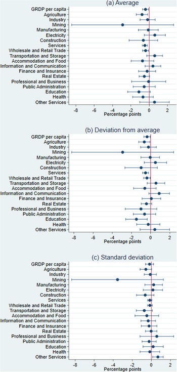
The effects of weather shocks on economic growth may vary according to the spatial aggregation of weather data. Damania et al. (Reference Damania, Desbureaux and Zaveri2020), for instance, reveal that at the smallest spatial resolution, there is a concave relationship between precipitation and GDP per capita growth. As the data are aggregated to larger spatial scales, however, the significance of the impact of precipitation becomes smaller until it ultimately disappears when aggregated at the country level. In this section, we aggregate the weather data at a larger spatial scale, administrative region level, and test whether fluctuations in weather affect GRDP growth rates. Then, to understand the channels through which the effects of weather shocks propagate through growth at the regional level, we examine the impact of temperature and precipitation shocks on the real growth rates of the GVA of agriculture, industry and services, along with the subsectors of each sector. Figure 1 shows the effects of temperature shocks, while figure 2 presents the effects of precipitation shocks. In both figures, all point estimates as well as their corresponding 95 per cent confidence intervals are from separate regressions of the growth in overall GRDP per capita and the growth in the GVA of its components. Panel (a) uses average levels, panel (b) deviations from the 20-year moving average historical norm and panel (c) standard deviations. All regressions control for region fixed effects and year fixed effects with robust Driscoll and Kraay (Reference Driscoll and Kraay1998) standard errors which allow for spatial dependence at arbitrary scales.
Effects of temperature shocks on GRDP by sectors and subsectors.

Effects of precipitation shocks on GRDP by sectors and subsectors.

As figure 1 shows, at the regional level, there is a negative relationship between temperature shocks and growth, although this link is not statistically significant. Looking across sectors, we find that a  $1^\circ\,\mathrm{C}$ increase in the standard deviation of temperature in a given year drags growth in agriculture by 6.4 pp (panel c). We also find that a
 $1^\circ\,\mathrm{C}$ increase in temperature, either in the average level (panel b) or deviation from its historical norm (panel c), reduces growth in services by 3.5–4.4 pp. Among services subsectors, education is the most sensitive to temperature shocks, with a
 $1^\circ\,\mathrm{C}$ increase in either average temperature or in its deviation from its historical norm depressing growth considerably in educational services by 20.6 pp. Also, health services are severely affected as the impact of a
 $1^\circ\,\mathrm{C}$ warming on the growth in human health and social work activities is in the order of 9.4 pp. Deviations of temperature from its historical norm also decreases growth in real estate services by 3 pp. On the other hand, growth in transportation and storage increases by 5–5.6 pp with a
 $1^\circ\,\mathrm{C}$ increase in either the average level or deviation from the moving average of temperature. We do not find a statistically significant relationship between temperature shocks and growth in industry. However, looking across subsectors under industry, we find that a
 $1^\circ\,\mathrm{C}$ increase in either the average level or deviation from historical norm of temperature increases growth in electricity by 7.5–8.6 pp. Growth in mining is reduced by 29 pp because of a
 $1^\circ\,\mathrm{C}$ increase in temperature variability.
While we do not find a statistically significant relationship between temperature and growth at the regional level, figure 2 shows that there is a negative and statistically significant relationship between precipitation and GRDP growth. A 1 mm increase in either the average level (panel a) or deviation from its historical norm (panel b) of precipitation decreases growth by about 0.4 pp. Looking across sectors, higher precipitation consistently drags agricultural production by 0.6–0.8 pp. Growth in services is also dampened by 0.4–0.5 pp for every 1 mm increase in the average level or deviation from moving average of precipitation. Among services subsectors, increased rainfall depresses growth in wholesale and retail trade as well as education. A 1 mm increase in either average precipitation or deviation from its historical norm hurts growth in wholesale and retail trade by 0.4 pp and education by 1.1–1.5 pp.
These findings are consistent with the channels of weather shocks documented by previous studies. Temperature and water are direct inputs into the biological processes of plant growth, hence the effects of weather shocks on income growth are clearest under the agriculture channel. A vast literature including Schlenker and Lobell (Reference Schlenker and Lobell2010) and Lanzafame (Reference Lanzafame2014) for Africa, Feng et al. (Reference Feng, Krueger and Oppenheimer2010) for Mexico and Welch et al. (Reference Welch, Vincent, Auffhammer, Moya, Dobermann and Dawe2010) for Asian countries finds consistently negative effects of bad weather shocks on agricultural output. Kotz et al. (Reference Kotz, Levermann and Wenz2022) reveal that increases in the number of wet days and in extreme daily rainfall cause huge reductions in growth rates of subnational units. They add that rainfall shocks dampen economic activity in services sectors for regions in high-income countries. Hsiang (Reference Hsiang2010), who measures the effects of temperature and cyclones in 28 Caribbean countries, finds that periods of unusually high heat have large negative effects for three of six nonagricultural sectors, two of which are service-oriented, and the remaining is industrial (mining and utilities). Dell et al. (Reference Dell, Jones and Olken2014) survey observational and experimental studies that show a strong negative relationship between temperature and labour productivity in services sectors such as call centres, bank workers, office workers, as well as students. Given the negative effects of high temperature on labour productivity, it is likely that these impacts could translate into reductions in aggregate output in services, including education, health and real estate services. Consistent with studies in the literature, we do not find statistically significant effects on industry growth as manufacturing industries or factories are likely less exposed to heat due to air conditioning as summarized in Dell et al. (Reference Dell, Jones and Olken2014). Indeed, we find that growth in electricity increases from elevated warming. Hsiang (Reference Hsiang2010) does not find a statistically significant impact of temperature on manufacturing output. Likewise, Otrachshenko and Popova (Reference Otrachshenko and Popova2022), who examine the channels behind the temperature-inequality relationship among Russian regions, find no statistically significant impact of temperature on relative wages in different industry sectors. The finding that more precipitation decreases wholesale and retail trade is aligned with the evidence that rainfall shocks disrupt the flow of inputs in the operation of enterprises.
3.3.2. Effects of the weather by rice-planting season
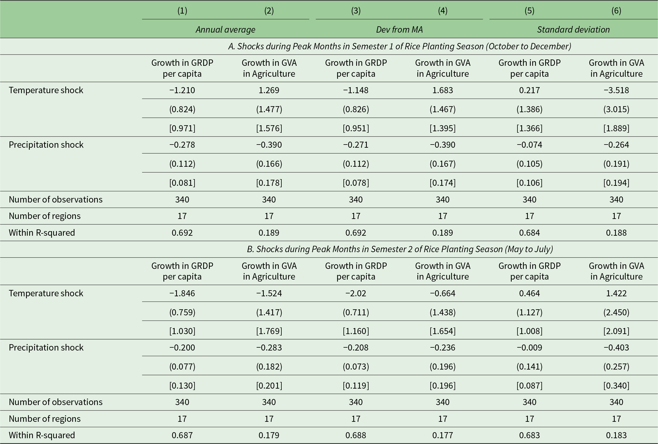
In table 4 and table A15, we further look into the agriculture channel by examining shocks during the peak and non-peak months of the rice-planting seasons in the Philippines, respectively. Using the derived rice planting window estimates of Gutierrez et al. (2019) for the regions in the Philippines, we aggregate the weather shocks that occurred during the planting season. For table 4, we use the peak months in the two rice planting semesters: semester 1 (from October to December) and semester 2 (from May to July). For table A15, we use the non-peak months: semester 1 (September and February) and semester 2 (April and August). For both tables, panel A shows the effects of weather shocks that occurred during semester 1, while those in panel B are the effects of the weather during semester 2. The odd-numbered columns present the effects on GRDP per capita growth, while the even-numbered columns show the effects of growth in GVA in agriculture. In table 4, we find that the agriculture channel of weather shocks propagates through growth mainly via shocks that occurred during the peak months of October to December (semester 1). A 1 mm increase in either the average level of deviation from moving average of precipitation during this season reduces agricultural production by 0.4 pp (columns 2 and 4 of panel A), and this translates into a 0.3 pp contraction in GRDP per capita growth (columns 1 and 3 of panel A). We do not find any statistically significant relationship between temperature shocks during semester 1 and growth, except for a 3.5 pp reduction in agriculture from a  $1^\circ\,\mathrm{C}$ increase in temperature variability in column 6, although the coefficient is weakly statistically significant. On the other hand, for temperature and precipitation shocks that occurred in semester 2 (panel B), although GRDP per capita growth decreases by 0.2-2 pp because of these planting season shocks (columns 1 and 3 of panel B), it is not likely through the agriculture channel as none of the coefficients in columns 2, 4 and 6 is statistically significant.Footnote 13 Table A15 confirms that agricultural productivity acts as a transmission channel as we do not find any meaningful effects of weather shocks that occurred during non-peak months in both semesters on the overall GRDP growth and the growth in agriculture (except for a positive effect of increased precipitation variability in semester 2 on growth in agriculture).
Effects of weather shocks during peak months of rice planting season on GRDP

Notes: The dependent variable for columns 1, 3 and 5 is the growth in GRDP per capita, while the dependent variable for columns 2, 4 and 6 is the growth in GVA in agriculture. All columns include region fixed effects and year fixed effects. Robust standard errors are in parentheses, while Driscoll and Kraay (Reference Driscoll and Kraay1998) standard errors which allow for spatial dependence at arbitrary scales are in brackets. Average temperature is in  ${}^{\circ}\,\mathrm{C}$, while average precipitation is in mm per year. Deviation from moving average (Dev from MA) refers to the deviations from their respective 20-year moving average historical norm. Standard deviation measures within-year variability.
4. Conclusion
Combining novel NTL data with high-quality atmospheric reanalysis, this paper examines the causal effects of temperature and precipitation shocks on growth in income per capita at the municipality level in the Philippines, the world’s most disaster-prone country, covering more than 1600 localities from different levels of economic development and climate zones over the period 2000–2020. Then, we test whether these effects persist in the medium run (i.e., growth effects) and analyse nonlinear effects. Lastly, we analyse the specific transmission channels of weather shocks.
Overall, our findings highlight the importance of understanding the distributional effects of climate change within countries, its underlying mechanisms, and how economic development policies can help shield poor municipalities from the vagaries of the weather. A caveat in our analysis is that while NTL is a strong proxy for local economic activity, it does not capture agricultural productivity well, as shown by Pagaduan (Reference Pagaduan2022). Moreover, Gibson et al. (Reference Gibson, Olivia, Boe-Gibson and Li2021) show that in less densely populated and less developed contexts, elasticities from Indonesia suggest that changes in GDP are approximately one-fifth of changes in nightlights. An avenue for future research points to exploring the extent to which policies and institutions can mitigate the sizable impact of weather shocks on the poor. Acevedo et al. (Reference Acevedo, Baccianti, Mrkaic, Novta, Pugacheva and Topalova2019) suggest that general economic development policies would complement any climate adaptation strategy. As with other developing countries, accelerating climate action and strengthening disaster resilience among localities, especially the poor ones, remains a major challenge in the Philippines. Thus far, the national government budget allocation for climate and disaster resilience has been inadequate, according to the Philippine Development Plan 2023–2028. The share of the budget for climate change adaptation and mitigation in the total budget declined from 6.99 per cent in 2017 to 5.77 per cent in 2022. At the local level, poor technical capacity of many LGUs to use information on climate change action and disaster risk reduction, coupled with limited financial resources, hinder effective implementation of local resiliency programs. For instance, disaster risk reduction and management funds were spent mainly on disaster response, recovery and rehabilitation. Strategies designed to help LGUs better access available financing platforms (such as the People’s Survival Fund) will boost climate and disaster risk resilience of communities, especially the poor.
Supplementary material
The supplementary material for this article can be found at https://doi.org/10.1017/S1355770X25100259.
Acknowledgements
I am grateful to the editorial board, two anonymous referees, Stephane Hallegatte, Matteo Lanzafame and Connie Bayudan-Dacuycuy for valuable comments and suggestions.
Competing interests
The author declares none.