




No CrossRef data available.
Trajectories of marijuana use from adolescence to young adulthood: Predictors and outcomes
Published online by Cambridge University Press: 01 December 2004
Abstract
Semiparametric group-based mixture modeling was used with data from an adolescent school sample (N = 1205) for three purposes. First, five trajectory groups were identified to characterize different patterns of change in the frequency of marijuana use across four waves of assessment during adolescence. These trajectory groups were labeled Abstainers, Experimental Users, Decreasers, Increasers, and High Chronics. Second, trajectory group comparisons were made across eight adolescent risk factors to determine distinctive predictors of the trajectory groups. Findings indicated, for example, that the High Chronic group, relative to the other trajectory groups, had higher levels of delinquency, lower academic performance, more drug using friends, and more stressful life events. Third, adolescent trajectory group comparisons were made across 10 risk behaviors in young adulthood (average subject age = 23.5 years) and the occurrence of psychiatric and substance abuse disorders. Findings indicated some consistency across adolescence to young adulthood with regard to risk factors, and specificity with regard to the prediction of disorders. Adolescent trajectory group membership was significantly associated in young adulthood with cannabis and alcohol disorders but not with major depressive disorders or anxiety disorders.This research was supported by a grant (R37-AA07861) awarded to Michael Windle from the National Institute on Alcohol Abuse and Alcoholism. An earlier version of this article was presented at the Michigan Symposium on Development and Psychopathology: Continuity and Discontinuity during the Transition to Adulthood, Ann Arbor, MI, June 14–15, 2002.
Information
- Type
- Research Article
- Information
- Copyright
- © 2004 Cambridge University Press
Marijuana remains a prominent substance of choice among adolescents and young adults, third only to alcohol and tobacco in terms of prevalence of use. Findings from national data such as the Monitoring the Future Surveys (Johnston, O'Malley, & Bachman, 2002) indicate lifetime rates of marijuana use at 49% among 12th graders, 40% among 10th graders, and 26% among 8th graders. Although marijuana is not typically considered a “hard drug” and is commonly perceived by the public as less harmful than many other illicit substances (e.g., crack, heroin), it is illegal, can lead to conviction and incarceration, and has been associated with a range of poor health outcomes (Kandel, 1984; Newcomb & Bentler, 1989). For example, findings from the National Institute of Justice's Arrestee Drug Abuse Monitoring Program indicated that across nine juvenile arrestee sites, 53% of juvenile male and 38% of juvenile female arrestees tested positive for marijuana (NIDA Research Report, 2002). Similarly, findings from the Drug Abuse Warning Network (Office of Applied Studies, 2002), a surveillance system for monitoring the health impact of drug abuse in medical emergency departments (ED), indicated that marijuana use was a contributing factor to an estimated 110,000 ED visits in the United States in 2001; about 15% of the patients were children between the ages of 12 and 17. Other studies (Tashkin, 1990) have indicated that the long-term abuse of marijuana may adversely impact immune system functioning and may contribute to increased risk for pulmonary problems (e.g., chronic coughs, bronchitis, emphysema) and cancer of the head, neck, and lungs.
In describing the research literature on marijuana use, it is important to distinguish between the different indicators or phenotypes that have been investigated. Marijuana phenotypes that have been studied include onset or initiation, frequency and/or level of use, chronicity or persistence of use across time, cannabis disorders, and cessation of use. It is important to distinguish these different marijuana phenotypes because there may be unique, or distinct, predictors of each, to complement predictors that may be common across two or more of the phenotypes (Glantz & Pickens, 1992; von Sydow, Lieb, Pfister, Hofler, & Wittchen, 2002). Knowledge of common and unique predictors of substance use and mental health phenotypes may provide a strong foundation for prevention science and for the development, implementation, and evaluation of intervention programs (Coie, Watt, West, Hawkins, Asarnow, Markman, Ramey, Shure, & Long, 1993).
In addition to the importance of distinguishing marijuana phenotypes and their common and unique predictors, it is also important to recognize that, with some notable exceptions (Kandel & Chen, 2000; Newcomb & Bentler, 1989), the majority of studies on marijuana use have used either cross-sectional research designs or two-wave longitudinal research designs with a relatively large number of years between years of assessment (von Sydow et al., 2002). These research design considerations are of significance because they constrain our knowledge about time-course issues related to marijuana use, and limit inferences about critical issues from a developmental psychopathology perspective such as distinguishing normative from nonnormative development, describing dominant intraindividual trajectories of marijuana use, identifying major risk and protective factors, and gaining insight into ongoing person–environment transactional processes (Cicchetti, 1993; Windle & Davies, 1999; Zucker, Fitzgerald, & Moses, 1995). In this article, we attempted to address some of these issues by focusing on changes in the frequency of marijuana use across four waves of assessment during adolescence, by identifying adolescent predictors of these changes, and by evaluating the associations between trajectories of adolescent marijuana use and cannabis (and other psychiatric) disorders about 5 years later in young adulthood.
Conceptual Model and Risk Factors for Adolescent Marijuana Use
The conceptualization that guided this research was based on a developmental psychopathology perspective (Cicchetti, 1993; Windle & Davies, 1999; Zucker et al., 1995) that emphasizes dynamic multiple factor influences on changes in marijuana use across multiple levels of analysis (e.g., biogenetic, individual, family, peer, school, neighborhood/community). Intrinsic to this perspective is the notion that temporal factors and dynamic processes related to intraindividual development are impacted both by proximal and distal determinants that may vary in their impact contingent on individual cumulative histories and current contextual exigencies. The trajectory analysis statistical procedure used in this study, and described subsequently, provides one method of addressing processes relevant to variation in intraindividual change. The current research has identified a number of risk factors across different levels for various marijuana phenotypes such as initiation, frequency, and level of use (Hawkins, Catalano, & Miller, 1992; Kandel & Chen, 2000; Newcomb & Bentler, 1988; Petraitis, Flay, & Miller, 1995). The multilevel domains for these risk factors have included dispositional (e.g., temperament) and interpersonal (e.g., family, peers) factors, contextual influences (e.g., neighborhood and community-level factors), and secular trends in the accessibility, potency, and price of marijuana.
In this article, we used eight predictors of changes in the frequency of marijuana use during adolescence. They included the individual-level variables of alcohol use, delinquency, and depressive symptoms; friend-level variables of percentage of friends using alcohol and other drugs; a family-level variable of perceived support from the family; a school-level variable of performance as indicated by grade point average (GPA); and an across-level variable of stressful life events. These risk factors for marijuana use have been supported in the literature (Bailey, Flewelling, & Rachal, 1992; Butters, 2002; Coffey, Carlin, Lynskey, Li, & Patton, 2003; Kandel, 1984; von Sydow et al., 2002); and, although not exhaustive either within or across levels of influence, they provide a useful set of predictors to examine the research objectives of this study.
As mentioned previously, in this article we investigated changes in marijuana use across adolescence. However, relative to the existing literature, there were two important differences in our research design and data analytic methods. First, we used four waves of data with 6-month intervals between waves to model growth, or intraindividual change, in the frequency of marijuana use. This contrasts with existing cross-sectional and two-wave longitudinal studies. Second, we used a statistical modeling procedure, semiparametric group-based mixture modeling (SGM), which enabled us to identify distinct trajectories of change. It is important that the SGM is consistent with recent conceptualizations in developmental psychopathology related to distinctions between variable-based and patterned-based (or person-oriented) approaches.
Variable-Based and Person-Oriented Approaches
Variable-based approaches typically rely on large sample, aggregate statistics (e.g., means, standard deviations) and standard linear or logistic regression models to make inferences about variables for the sample as a whole, or disaggregated by some major sociodemographic factor (e.g., by ethnic group or by gender group). Studies that have adopted this approach are dominant in the field of substance use studies and have made significant contributions to the scientific literature. An alternative, but complementary, conceptual and methodological approach that has attempted to address the dynamic, multifactorial, and heterogenous nature of the development of substance use and abuse and other domains of dysfunction (e.g., poor mental health, criminality) has been referred to as the person-oriented, or pattern-based approach (e.g., Cairns, Bergman, & Kagan, 1998; Hinde & Dennis, 1986; Magnusson & Bergman, 1988). The person-oriented approach, which explicitly recognizes the importance of variation in intraindividual change trajectories, seeks to identify significant subgroups of “individuals” (or persons) who share a certain pattern of characteristics (e.g., multiple vs. single problem youth), and to then examine such subgroups across time (e.g., in young or middle adulthood) for differences with regard to the expression of a substance use or other psychiatric disorder, or serious levels of substance use or mental health problems. The following description by Magnusson and Bergman (1988, p. 47) succinctly captures the significance of the complementary, person-oriented approach within a person–environment interactional perspective:
According to this view, development is regarded as a process in which cognitive-affective and biological factors in the individual, and distal and proximal factors in the environment, are involved in a constant, reciprocal interaction … The patterning of various aspects of individual functioning in an individual represents a partly specific mosaic of psychological, biological and environmental (situational) factors … Thus, what is characteristic of a certain individual at a certain stage of development is the patterning of relevant factors, a patterning that is the result of a life history of interaction processes.
Although historically the origins of the variable- versus person-oriented approaches can be traced to long-standing scientific and philosophical controversies over the continuous versus discrete nature of the world, in recent years more discussion has been precipitated by developmental psychologists and psychopathologists in the United States and Sweden (Block & Robins, 1993; Cairns et al., 1998; Chassin, Presson, Sherman, & Edwards, 1994; Magnusson & Bergman, 1988). The fundamental argument for the need of a person-oriented approach to complement a variable-based approach is that the considerable heterogeneity associated with different trajectories of intraindividual change, influenced by initial individual differences (e.g., in genetically influenced temperament propensities), and differences in experientially based life histories (e.g., in parent–child relations, major life events such as parental divorce), may not be adequately captured by aggregated statistics. For example, in a longitudinal panel design, aggregated statistics may suggest that the average change (i.e., mean level) of marijuana use may remain approximately equal over three waves of measurement, leading a researcher to conclude that the behavior under study, marijuana use, manifested a high level of continuity across time. However, it is possible (hypothetically) that 50% of the sample manifested a pattern of significantly increasing levels of marijuana use across time, whereas the remainder of the sample manifested a pattern of significantly decreasing levels of marijuana use across time. The two significant trends (increasing for one group and decreasing for the other) could, in effect, cancel each other out and the conclusion drawn (based on aggregate data) would be that there was continuity (or no change) across time, even though there was significant change if groups had been identified according to the patterns of change reflected in the variation of their individual trajectories.
Magnusson and Bergman (1988) provided a useful illustration of the value of the pattern-based approach in their prospective longitudinal study of Swedish youth from ages 13 to 18–23 years. Briefly, these authors used a cluster analytic procedure to identify six patterns of maladjustment among boys, rated by teachers, at age 13 years. Maladjustment indicators included a range of variables (e.g., aggression, motor restlessness, poor concentration, poor peer relations) that have been identified as major risk factors in the larger literature of developmental psychopathology. Some of the clusters consisted of multiple problem profiles, whereas others were dominated by a single problem. Magnusson and Bergman then used the identified cluster groups to investigate differences in late adolescent/adulthood functioning (ages 18–23 years), based on official record data, with regard to alcohol abuse, criminality, and psychiatric care. The findings indicated significant levels of association for individuals in the multiproblem clusters and the outcome variables, but not for the single problem clusters. For example, boys with poor peer relations or underachievement at age 13 years were not at high risk for maladjustment by age 23 years unless these behaviors were displayed within the context of other (multi-) problem behaviors in early adolescence. These findings, based on identified individual-level clusters, would not necessarily have been evident in an aggregated sample, linear regression model; the person-oriented analyses revealed that these maladjustment indicators (of poor peer relations and underachievement) were conditionally predictive of young adult dysfunction only within the context of other multiproblem behaviors.
Schulenberg, Wadsworth, O'Malley, Bachman, and Johnston (1996) have also provided a useful application of the person-oriented approach in their four-wave, prospective longitudinal study of risk factors predicting changes in binge drinking (defined as five or more drinks in a row during the past 2 weeks) during the transition from adolescence to young adulthood. Schulenberg et al. used cluster analysis to identify several binge drinking patterns with regard to the four waves of data. For example, a chronic binge drinking trajectory was identified for subjects who had engaged in binge drinking at all four waves of data collection; a decreased binge drinking trajectory was identified for subjects who frequently binged at Wave 1, but decreased to no frequent binge drinking by Wave 4; an increased binge drinking trajectory was identified for subjects who reported no frequent binge drinking at Wave 1, but increased to frequent binge drinking by Wave 4. The authors then conducted planned comparisons among some of the identified subgroups to evaluate adolescent predictors that may account for changes in the growth trajectories into young adulthood. For instance, the Chronic and Decreased groups had high levels of binge drinking in their senior year of high school (approximately four binge drinking episodes in the last 2 weeks); however, across time the Chronic group persisted in their high levels of binge drinking whereas the Decreased group significantly reduced their levels of binge drinking. It is important to note that these two groups also did not differ in their senior year on a number of other variables (e.g., antisociality/rebelliousness, GPA, time spent with friends) that may have accounted for different binge drinking trajectories. The findings of the study indicated that being female, having higher self-efficacy and work readiness, less drinking to get drunk, and greater loneliness significantly differentiated those youth who decreased their binge drinking relative to those who persisted in their binge drinking.
The findings of the person-oriented approach by Schulenberg et al. (1996) and Magnusson and Bergman (1988) provided valuable qualifications to the more aggregate, sample-based statistics by extracting information about relatively homogenous subgroups within the larger matrix of the total sample data. The identification of such subgroups facilitated inquiry into more refined conditional relationships that may not have been evident using more standard linear modeling approaches (e.g., multiple regression), even if interaction terms were included in the equations. Some of the relationships identified with the person-oriented approach may be nonlinear, and actually assume a quite complex nonlinear functional form. The use of the person-oriented approach is consistent with conceptual frameworks that emphasize alternative pathways for expression of substance use and mental health disorders, and provides a straightforward method for assessing the generality versus specificity of influences. For example, in the Schulenberg et al. study, one could hypothesize and test statistically whether the same (or different) factors contributed to increases versus decreases in binge drinking. The person-oriented approach may also resonate well with psychiatrists and other mental health professionals who are more accustomed to viewing individuals in life situations, and are often confused by, or view as irrelevant or limited, the findings of variable-based studies. The proposal here is that person-oriented approaches provide a useful complement to variable-based approaches. Further, the person-oriented approach may be quite useful in untangling some of the heterogeneity associated with dynamic, multifactorial phenotypes such as marijuana use.
The existing longitudinal studies of marijuana use among adolescents have been useful in contributing to the more general notion that many behaviors exhibited during adolescence, including marijuana use, exhibit considerable time-course heterogeneity (Kandel & Chen, 2000). That is, more static, disease or trait-like perspectives are not adequate to account for temporal variation in marijuana use during adolescence. As a corollary, it is argued that more developmentally dynamic perspectives are needed to account for the temporal heterogeneity of many behaviors, including marijuana use, expressed across the transition from adolescence to young adulthood (Schulenberg & Maggs, 2002; Windle & Davies, 1999; Zucker et al., 1995). Upshots of this more dynamic, developmental orientation have included more of a focus on intraindividual change across time and the adoption of person-centered models to complement existing aggregate, variable-oriented models (Cairns et al., 1998; Magnusson & Bergman, 1990; Schulenberg et al., 1996).
SGM and Objectives of Study
To accommodate developmental dynamic models of substance use and mental health across time, it is necessary to apply statistical models that are best able to capture time-course variation within subjects across time. An array of alternative longitudinal models has emerged in recent years to address issues related to the modeling of repeated measures data (Bryant, Windle, & West, 1997; Collins & Sayer, 2001).
Among the more recent analytic models to capture individual time-course variation consistent with the person-oriented approach are growth mixture distribution models (Muthén & Muthén, 2001; Nagin, 1999). The general concept guiding growth mixture distribution models is that cross-time trajectories may be more optimally measured as subpopulations of growth curves rather than as a single population representing the overall growth parameters of the entire population. This notion is operationalized with K representing a latent class variable of c classes or trajectory groups. These c trajectory groups may vary in number and each may vary in shape (within the mathematical and statistical constraints of the data).
Two of the most widely used programs to conduct growth mixture modeling are Mplus (Muthén & Muthén, 2000) and SAS PROC TRAJ (Jones, Nagin, & Roeder, 2001). Both programs enable mixture modeling of unobserved heterogeneity in a sample where subjects are numbers of different subpopulations, or trajectory groups, that are inferred from the observed data. Presently, not much is known about the relative benefits (and limitations) of using Mplus or PROC TRAJ for research applications with categorical manifest indicators that are distributed in ways that deviate from underlying model assumptions related to a normal probability density function (but see Bauer & Curran, 2003). A flexible feature of PROC TRAJ is the option to specify statistical models and associated distributions that may more closely correspond with the observed data. In our application with marijuana use, there were a large number of zero values and among those who did engage in marijuana use, a count variable was created to indicate the number of times that each subject engaged in marijuana use. Given these two characteristics (i.e., a high number of zeros and count data), the zero-inflated Poisson (ZIP) model available within PROC TRAJ (and not Mplus) seemed to be the most consistent with our data and was selected to model the unobserved heterogeneity (Lambert, 1992).
In this study, a growth mixture distribution model was used for four purposes. First, most prior longitudinal research on marijuana use has been restricted to two-waves of data collection, thereby restricting the evaluation of more complex patterns of across time changes. The growth mixture distribution model was used in this study to identify distinctive longitudinal trajectories of marijuana use across four-waves of data collected during adolescence. Second, most of the previous research on marijuana use among adolescents has focused on a single event (e.g., onset, cessation) or a simple two-wave change score for marijuana use. The growth mixture distribution model in this article is used to model rates of change for subpopulations that may vary not only in initial levels of use and in rate of change, but also in the direction (e.g., increasing, decreasing) and shape of change (e.g., linear, quadratic). Third, predictors measured at Wave 1 were analyzed to determine if identical or different risk factors were equally likely to be associated with the alternative longitudinal trajectory groups. Fourth, the longitudinal trajectory groups were compared to assess different associations with outcomes in young adulthood (e.g., psychiatric and substance abuse disorders, level of educational attainment).
Method
Sample
The data used in this study were collected as part of a larger, multiwave panel design focused on vulnerability factors and adolescent substance use. We refer to the study by the acronym LAT, which stands for Lives Across Time: A Longitudinal Study of Adolescent and Adult Development. The LAT is currently in its 16th year of funding and sixth wave of data collection. The study was initiated in 1988 as a longitudinal study of adolescents, but in subsequent years became a triadic-family (mother, father, child) study. The original primary objective of the LAT was to assess the initiation, maintenance, and continuation (or termination) of alcohol and other substance use during the high-school years in relation to a range of vulnerability, or risk, factors (e.g., temperament, peer substance use, family history of alcoholism). Data were collected within the adolescents' high school setting and the overall student participation rate was 76%. The initial wave of assessment occurred during the Fall semester of the teens' 10th- and 11th-grade years. Waves 2 through 4 data collection occurred every 6 months thereafter, with Wave 2 data being collected in the Spring semester of Year 1, and Waves 3 and 4 being collected in the Fall and Spring semesters of Year 2, respectively, when adolescents were in 11th and 12th grades. Because of time constraints associated with testing in classroom settings, and the desire to measure a broad range of risk and protective factors and health outcomes, not all measures were assessed at all four waves of measurement.
The initial sample consisted of 975 high school sophomores (53%) and juniors (47%) recruited from two homogeneous suburban public high school districts in western New York. Fifty-two percent (n = 517) of the sample was female and 48% (n = 458) was male. The average age of the respondents at the first occasion of measurement was 15.54 years (SD = 0.66) and 98% were White. Seventy percent of the sample was Catholic, 18% Protestant, and 12% other. Ninety-six percent of the fathers and 43% of the mothers were employed full time outside the home (37% of mothers were employed part-time outside the home). Fathers completed an average of 13.79 years of education (SD = 2.39) and mothers completed an average of 13.55 years (SD = 2.01). The average number of children per family was three. The median family income was about $40,000, with only 3% of the sample reporting family income less than $12,000. Eighty-eight percent of the adolescents' primary caregivers were currently married, 12% were divorced, and 1% were widowed. The retention rate at the second occasion of measurement (6 months later) was 93%. Sample retention across the first four waves of measurement was uniformly high, in excess of 90%.
A supplemental sample of 235 adolescents participated at the second, but not the first, wave of measurement and was eligible to participate at subsequent waves of measurement. These supplemental subjects were added to the study to increase the sample size for some relatively low base rate variables (e.g., family history of alcoholism) of interest to the objectives of the larger federally funded project. Statistical comparisons on sociodemographic variables (e.g., parental education level, income) and adolescent problem behaviors (e.g., alcohol use, delinquent activity) indicated that the supplemental sample did not differ in any systematic way from those subjects who participated initially at the first measurement occasion. Because active informed consent procedures were used in this study, information on nonparticipants was not available; hence, it is unclear how representative the participating sample was relative to the total eligible sample except on major sociodemographic variables (e.g., gender and ethnic group composition), which did not reflect participant bias. It has been determined, however, that the drinking and substance use practices, and rates of suicidal ideation and attempts, among adolescents in this sample were highly similar to findings in national survey studies (see Reifman & Windle, 1995; Windle, 1996).
Seventy-one percent of the primary caregivers (92% female) of the participating adolescents completed and returned mail survey materials that contained questions about sociodemographic characteristics (e.g., income, parental educational attainment) and family history of alcoholism, mental health problems, and regular smoking. For those primary caregivers who did not return the mail survey, selected information (e.g., income, regular smoking) was collected via telephone calls. This resulted in complete response information for these parent variables for all but 26 of the families participating in the study.
Subsequent to the four waves of assessment during adolescence, the study was modified in two major ways: (a) mothers and fathers were invited to participate in the study as target subjects along with their young adult child, rather than simply as a reporter of adolescent behaviors; and (b) data collection changed from a large group, survey format to individual interviews in the home or at the worksite of the investigators. For the Wave 5 data collection, the self-report mode of administration was retained for many of the measures used in Waves 1–4, such as alcohol, marijuana, and other substance use, Center for Epidemiologic Studies Depression Scale (CES-D; Radloff, 1977) depressive symptoms, reports of sexual behavior, and romantic involvement. This was done to eliminate, or minimize, the possible impact of change in mode of administration on these repeatedly assessed measures. However, computer-assisted interviews were used to collect information on psychiatric diagnoses (e.g., cannabis dependence and abuse), sociodemographic characteristics, and health-related data (e.g., medical history, reproductive problems).
The Wave 5 data collection occurred when the average age of the young adults was 23.5 years. We attempted to contact all 1216 subjects, even if they only participated at one wave during Waves 1–4 adolescent assessment. At least one (of three possible) subjects from 940 households participated in the study, including 829 young adults. The participation rate for young adults was 68% based on the number participating divided by the number we attempted to contact; the participation rate was 79% if the denominator was the number of participants at Wave 4. Despite the use of numerous tracking efforts (e.g., Department of Motor Vehicles, State Credit Bureau), 233 young adults could not be tracked. For these 233 young adults, we could obtain no contact information on 94, we contacted parents for 60, but parents either did not know or refused to provide us with contact information, 15 were in the military, incarcerated, or out of the country, 41 initially agreed to participate but after numerous rescheduling cancellations were dropped (for this wave), four requested that we contact them later due to current demands (e.g., new baby), and for 19 cases we repeatedly left messages via voice-mail messages but were unable to confirm if this was the telephone number of the targeted participant. Three foreign exchange students who had participated during adolescence and then returned to their native country were not followed-up, and there had been one homicide.
Attrition analyses were conducted at Wave 5 among Participants (n = 829), Refusers (n = 154), and Nonlocatables (n = 233). There were significant differences with regard to gender, χ2 (2) = 32.98, p < .001, as proportionally more females (75.4%) than males (61.4%) participated at Wave 5 (note that this percentage included Nonlocatables). Comparisons among the three participant status groups (Participants, Refusers, Nonlocatables) for separate gender groups were then made with Wave 2 assessments for four sociodemographic variables (family income, number of children in the family, and each parent's highest educational attainment), two family variables (family cohesion and perceived family social support), two deviant peer variables (percentage of alcohol and drug using friends), five problem behaviors (tobacco, alcohol, marijuana, and other illicit drug use, general delinquency), emotional functioning (depressive symptoms), academic performance (GPA), and number of stressful life events. Of these 32 comparisons (16 for each of the gender groups), two were statistically significant for males (Nonlocatables differed from Participants in that they had a higher percentage of alcohol using friends [70 vs. 59%] and lower perceived family social support; effect size [ES] = .31) and three were statistically significant for females (Nonlocatables differed from Participants in that, on average, they reported more stressful events in the last 6 months [7.6 vs. 6.5] and higher average rates of delinquency; ES = .49). In addition, among females, Participants differed significantly from Refusals in that Participants had higher GPAs (ES = .26). The participation status groups did not differ significantly on the remaining 27 statistical comparisons, and it is thus concluded that attrition bias is quite minimal for males and females, though the Nonlocatable females had significantly higher levels of delinquency and stressful life events during adolescence than the Participating females, although not higher levels of substance use, deviant peers, or depressive symptoms, or a lower GPA or poorer family relationships.
Measures
Marijuana use included the self-reported frequency of using marijuana/hashish during the last 6 months using 7-point Likert scales that ranged from never used to used every day. Marijuana use was measured at all occasions of measurement. The validity of self-reports of substance use has been supported in numerous research studies (Oetting & Beauvais, 1990; Winters, Stinchfield, Henly, & Schwartz, 1991).
Depressive symptoms
Depressive symptoms were assessed at all occasions of measurement using the CES-D (Radloff, 1977). The CES-D consists of 20 self-report items and provides a unitary measure of current depressive symptoms. Adolescents were asked to indicate how many days during the past week they experienced the emotions or behaviors indicated in each of the items. Items included “I thought my life had been a failure,” “I felt that everything I did was an effort,” and “I felt lonely.” Serious depressive symptomatology was indicated by a criterion score of ≥23 (Roberts, Andrews, Lewinsohn, & Hops, 1990). The internal consistency estimate for the CES-D with this sample was ≥.90 at each wave, and these alpha levels are consistent with prior research (e.g., Radloff, 1977; Roberts et al., 1990).
Perceived social support from family
Adolescents completed the perceived social support from family measure, which assesses the amount of perceived emotional support provided by the family (Procidano & Heller, 1983). The measure consists of 20 items with four response options ranging from generally false to generally true. Examples of survey items include “My family gives me the moral support I need,” “Members of my family are good at helping me solve problems,” and “My family is sensitive to my personal needs.” The response format of this measure was modified to a four-response option format from the original dichotomous response format (plus a “Don't know” response option) proposed by Procidano and Heller to increase the discriminative utility of the measure (Windle & Miller–Tutzauer, 1992). The internal consistency estimate for this measure at Time 1 with this sample was .95.
Delinquent activity was measured with 16 items used in prior delinquency research (e.g., Elliott, Huizinga, & Menard, 1989). A 6-point Likert scale (never, once, 2–3 times, 4–5 times, 6–9 times, 10 or more times) was used for each item in reference to the last 6 months. The alpha level for the 16 items at Time 1 was .75 and test–retest reliability was .70. Items varied in terms of severity of offense and included skipped school, hit teacher or parent, stole something that was valued at more than $20, beat up someone, destroyed public property, was suspended from school, and so on.
Alcohol consumption was measured with a standard quantity–frequency index (QFI) that assesses beer, wine, and hard liquor consumption in the last 30 days (Armor & Polich, 1982). Alcohol use was measured at all occasions of measurement. Respondents were asked how often they usually had each beverage in the last 30 days (responses on a 7-point scale from never to every day), and, when they had the beverage, on average how much they usually drank (10-point scale from none to more than 8 cans/bottles/glasses, etc., depending on the beverage). The QFI, based on all three beverages, provides a measure of the average number of ounces of ethanol consumed per day in the last month.
Percentage of friends who use alcohol and other drugs during adolescence
Adolescents were requested to indicate the number of adolescents that they considered friends. Over 99% of adolescents reported at least one friend, with most reporting five or more. Adolescents were then requested to indicate how many of these friends consumed alcohol. Percentage scores were calculated by dividing the number of alcohol using friends by the total number of friends and multiplying the dividend by 100, with a possible range of 0–100%. A similar procedure was used to calculate the number of illicit (e.g., marijuana, cocaine) drug using friends. These measures were administered to one of the schools at Wave 2 and to two of the schools at Wave 3 (6 months later).
GPA and educational attainment
Adolescents were requested to report their cumulative GPA with the following item, “What grades do you usually get in school?” This item had a 7-point response format from mostly As to mostly Ds and Fs. The Pearson correlation between adolescents' reports of their GPA and official high-school records (that used a somewhat different measurement scale) was .78. Therefore, this self-report item was judged as valid for assessing GPA. In young adulthood (Wave 5), participants were requested to report on the number of years of education that they had completed, with the completion of high school representing 12 years, BA or BS college degree representing 16 years, and so forth.
Major stressful life events during adolescence
A list of 29 undesirable life events was constructed by modifying the brief (24-item) form (Forman, Eidson, & Hagan, 1983) of the Adolescent Life Change Event Scale (ALCES) of Yeaworth, York, Hussey, Ingle, and Goodwin (1980) as detailed by Windle (1987). Events were sampled from multiple social stress domains: family (e.g., hassling with parents), school (e.g., failing one or more subjects), interpersonal (e.g., breaking up with a close personal friend), and intrapersonal (e.g., getting badly hurt or sick). Participants were asked to report whether or not each life event had occurred during the last 6 months.
Major stressful life events in young adulthood
A total of 46 life events adopted from the Holmes and Rahe measure (Holmes & Rahe, 1967) were used to assess stressful life events. Events were sampled from multiple age-appropriate domains: family (e.g., separated or divorced from significant other), work (e.g., fired, received a pay cut), financial (e.g., took out a large mortgage, having financial difficulties), and health related (e.g., serious illness or injury). Participants were asked to report whether or not each life event had occurred during the last 12 months.
Friends' alcohol and other substance use in young adulthood
Four questions were asked about the alcohol and other substance use practices of the young adults' current close friends. These included how many of these close friends drank regularly, were heavy drinkers, used marijuana, and used illicit drugs.
Family cohesion
The 10-item family cohesion subscale of the Family Adaptability and Cohesion Evaluation Scale, 3rd ed. (Olson, Portner, & Lavee, 1985) was used to assess emotional attachment to the family in young adulthood (Wave 5). The family cohesion scale had an internal consistency estimate of .92.
Psychiatric and substance abuse disorders
DSM-IV disorders were derived in the young adulthood interview via the World Health Organization (WHO) Composite International Diagnostic Interview (WHO-CIDI; WHO, 1997). Reliability data for the WHO-CIDI have been reported (WHO, 1997); and the disorders assessed in this study included alcohol and other substance abuse disorders, major depressive disorders, and several anxiety disorders (phobias, generalized anxiety, and panic). Some comparisons were made between the prevalence of disorders in our sample and those obtained in the National Comorbidity Study (NCS; Kessler, McGonagle, Zhao, Nelson, Hughes, Eshleman, Wittchen, & Kendler, 1994), although there are some differences between these studies with regard to sampling frame and diagnostic system (i.e., DSM-III-R in the NCS and DSM-IV in our study). Nevertheless, there were similarities in the prevalence of disorders and comorbidity across the samples for comparable age, gender, and racial/ethnic groups. For example, 48% of the NCS sample reported at least one lifetime disorder and the mothers and fathers in our sample reported rates of 50 and 52%, respectively. Young adults had a somewhat higher prevalence of disorders (57%), but such findings are consistent with the NCS in reporting cohort trends toward higher rates of disorders among younger adults. Similarities were also found for specific disorders, such as a rate of 30.5% for anxiety disorders among women in the NCS and 31.7% among mothers in our sample.
Procedure
Subsequent to receiving approval from school administrators to conduct the study, schools provided a mailing list of the addresses of 10th and 11th graders. A packet of materials, including a letter of introduction by the principal, a description of the study, and informed consent forms, was mailed to adolescents and their parents. Those individuals willing to participate in the study were requested to sign the informed consent form (both adolescent and one parent) and return it to the investigator in a self-addressed, stamped envelope. Confidentiality was also assured with a Department of Health and Human Services Certificate of Confidentiality. Teachers made announcements about the study in home classrooms. Adolescents completed survey materials in large groups (e.g., 40–50 students) in their high school setting. A trained survey research team administered the survey to adolescents, and neither teachers nor school administrators were in the room during the time the students completed the surveys. The survey took about 45–50 min to complete and subjects received $10.00 for their participation. A make-up date for testing was arranged for participants who were absent or unable to participate on the regularly scheduled day of testing. A similar procedure was used at each wave of measurement. Survey testing occurred in October and April of successive years.
The young adulthood interviews were conducted via one on one interviews either in the subjects' home or at the host institute of the investigators. Subjects were paid $40 to complete an interview that lasted approximately 2 hr. The data collection procedures were computerized and administered via computer-assisted personal interviews.
Analysis strategy
Data analysis proceeded in two stages. In the first stage, we used SGM, a form of growth mixture distribution modeling to identify distinct developmental trajectories of marijuana use during the middle adolescent years. In the second stage, we used other statistical procedures (e.g., analysis of variance [ANOVA], contingency table analyses) to make comparisons among the identified adolescent marijuana trajectory groups on precursors, correlates, and young adult consequences. Note that some programs such as Mplus (Muthén & Muthén, 2001) provide greater latitude in the specification of latent growth mixture models that incorporate covariates and outcomes than the program (Jones et al., 2001) used in this study. However, the ZIP distribution model available in the program we used (and not available in Mplus) seemed more consistent with our data, and as will be illustrated subsequently, provided a high degree of classification accuracy.
The SGM approach (Jones et al., 2001; Nagin, 1999) was developed to complement two well-known methods for analyzing developmental trajectories, namely, hierarchical modeling (e.g., Bryk & Raudenbush, 1992; Goldstein, 1995) and latent growth curve modeling (e.g., McArdle & Epstein, 1987; Willett & Sayer, 1994). Both methods estimate a growth curve for the given sample and capture individual differences in growth by allowing for continuous variability of the growth factors (i.e., estimation of growth factor variation). The SGM approach, in contrast, assumes that the given population is composed of a mixture of distinct subgroups, each defined by a prototypical growth curve. Because this method allows for cross-group differences in the shape of trajectories, it is especially suited for identifying and modeling heterogeneity in types of developmental trajectories within a given sample (Nagin & Tremblay, 1999).
The SGM models were estimated with a customized SAS macro developed by Jones and colleagues (2001) and Nagin (1999). It is important that SGM fits semiparametric (discrete) mixtures of censored normal, uncensored normal, regular Poisson, ZIP, and Bernoulli distributions to longitudinal data. Model parameters are estimated with a maximum likelihood estimator that allows for missing values in the longitudinal data and time-dependent covariates. Thus, SGM makes full use of available data and does not lose information through listwise deletion of data (Jones et al., 2001). Model selection requires determination of the number of groups that best describes the data. In SGM, a k group model is not nested within a k + 1 group model, and therefore it is not appropriate to use the likelihood ratio test for model selection. Instead, the Bayesian Information Criterion (BIC) is used as a basis for selecting the optimal model, because it can be used for comparison of both nested and unnested models (Kass & Raftery, 1995; Raftery, 1995). Generally, the model with the smallest absolute BIC value is chosen. Note that the BIC criterion tends to favor models with fewer groups because it rewards parsimony.
Results
Identification of different trajectories of marijuana use
The SGM approach was used to identify subgroups with distinct developmental trajectories of marijuana use during the middle adolescent years. The trajectories were modeled using the ZIP model. This model is particularly useful for modeling the conditional distribution of count data given group membership when there are more zeros than expected under the Poisson assumption (Lambert, 1992). This is common in antisocial and abnormal behavior that is typically concentrated in a small fraction of a given sample. Specifically, the model takes into account that individuals may enter periods of dormancy during which the probability of marijuana use is strictly zero. This zero-inflation parameter (or intermittency parameter) may or may not change with age (for some individuals, the dormancy period may last their whole life). During periods of activity, a Poisson model is used to describe the probability distribution of the number of times that marijuana was used per month. A more detailed description of the ZIP model can be found in Roeder, Lynch, and Nagin (1999).
We tested one-, two-, three-, four-, five-, and six-group models1
ZIP models can be difficult to fit to the data. In particular, the procedure may find only a local minimum; hence, it is critical to specify start values (Jones et al., 2001). We followed this recommendation and estimated all models using different sets of start values.
Results of semiparametric, group-based modeling

Figure 1 shows the fitted growth curves for the five marijuana usage trajectory groups. These trajectory groups are Abstainers, Experimental Users, Increasers, Decreasers, and High Chronics.2
The Abstainer, Experimental User, and High Chronic groups were modeled with an intercept factor, the decreaser group with a linear growth curve, and the increaser group with a quadratic growth curve. Other model specifications (i.e., trajectory shapes) were also tested, but this model proved to be the most parsimonious variant and achieved the best model fit. The estimated growth factor means were as follows: The intercept factor mean of marijuana use was −2.90 (t = −32.50, p < .001) for the Abstainers, 0.44 (t = 6.99, p < .001) for the Experimental Users, and 3.08 (t = 65.22, p < .001) for the High Chronics. The Decreasers had an intercept and linear factor mean of 6.22 (t = 13.23, p < .001) and −3.18 (t = −7.83, p < .001), respectively. For the Increasers, the intercept, linear, and quadratic factor had a mean of −33.18 (t = −4.84, p < .001), 49.57 (t = 4.62, p < .001), and −17.10 (t = −4.09, p < .001), respectively. Finally, the zero-inflation parameter did not change over time and had an intercept of −2.46 (t = −15.26, p < .001). The significant intercept indicated that there was statistically significant variation in the probability of marijuana use (yes vs. no) at Wave 1 (where the Intercept was scaled as the initial time point). The nonsignificant change parameter indicated that, on average, the probability of marijuana use versus nonuse remained constant across time.

The trajectories of marijuana use.
Given that there was some variation in the age of initial participation in this study, and some variation in the interval between Wave 4 and Wave 5 participation, we created an age difference (AD) variable (Wave 5 age–Wave 4 age) and made statistical comparisons on several variables to determine if the AD variation was statistically significant. The AD variable did not differ significantly across the five marijuana trajectory groups, F (4, 724) = 0.42, p > .05, and was not significantly correlated with any of the following Wave 5 variables: quantity–frequency of alcohol use, CES-D depressive symptoms, number of stressful life events, family cohesion, number of close friends who drink regularly, number of close friends who use marijuana, or number of friends who use illicit drugs other than marijuana. Hence, the AD variable was not included in subsequent analyses.
Adolescent risk factors and trajectory groups
Table 2 summarizes findings from a series of ANOVA models in which Time 1 adolescent behaviors (or Times 2 and 3 with regard to friend alcohol and drug use) were compared across the five trajectory groups.3
From a time-ordering perspective, the trajectory groups are the dependent variables and the predictors are the independent variables. However, ANOVA models were used for clarity of presentation and ease of computing post hoc comparisons using a conservative procedure. In addition to the ANOVA models, we also conducted a multinomial logistic regression model in which trajectory groups were specified as the dependent variable. The substantive findings across the ANOVA and multinomial logistic regression analysis were highly similar. For example, for the multinomial logistic regression model, the three largest chi-square statistics were for the variables of Friends' drug use, Alcohol use, and Delinquent activity. The F statistics for the ANOVA models (see Table 2) are also the highest for those three variables. Overall classification from the multinomial logistic regression model varied contingent on the arbitrarily designated referent group, but it ranged from 85 to 87%.
One-way ANOVAs for Time 1 adolescent behaviors by marijuana trajectory group

Young adult risk behaviors and psychiatric disorders
Table 3 provides a summary of the distribution of trajectory groups for Waves 1–4 and Wave 5 (the young adulthood follow-up). A statistical test for attrition indicated that there was not differential attrition across the five trajectory groups (χ2 with 4 df = 7.54, ns). In addition, comparison of trajectory groups by gender indicated no significant differences (χ2 with 4 df = 1.83, ns).
Representation at Waves 1–4 (W1–W4) and Wave 5 (W5) for trajectory groups

The prevalence of lifetime psychiatric and substance abuse disorders by adolescent marijuana trajectory groups is summarized in Table 4. Clearly, High Chronics have the highest prevalence of Cannabis Disorder, as would be anticipated via a continuity model; however, the prevalence of Cannabis Disorders was also relatively high among Increasers, Decreasers, and Experimental Users, and over 12% of Abstainers met criteria for a cannabis disorder by young adulthood. This pattern of findings suggests a fair amount of discontinuity in cannabis use from adolescence through young adulthood for a substantial portion of the sample, with different adolescent trajectory groups associated with higher or lower levels of continuity/discontinuity. A statistically significant difference was also indicated for the lifetime occurrence of an alcohol disorder across the trajectory groups, with marijuana abstainers having the lowest prevalence of alcohol disorders.
Prevalence of lifetime psychiatric disorders in young adulthood by adolescent marijuana use trajectory groups

Comparisons among trajectory groups for young adult behaviors that largely parallel those assessed in adolescence (see Table 2) are summarized in Table 5. The findings indicated that the High Chronics were significantly higher with respect to current marijuana and alcohol use, number of friends using illicit drugs, and lower levels of educational attainment. The Increasers also reported higher levels of current marijuana use and higher levels of friends using marijuana and illicit drugs, although there was no decrement in educational attainment.
One-way ANOVAs for Time 5 young adult behaviors by marijuana trajectory group

Because marijuana use may have changed in young adulthood, thereby yielding the distal influences of adolescent marijuana use trajectories as less important than the proximal influence of current marijuana use, we additionally specified one-way analysis of covariance models for the Wave 5 young adult behaviors presented in Table 5 and used current (i.e., Wave 5) marijuana use as a covariate. This was critical for determining if the adolescent marijuana use trajectories remained statistically significant for the Wave 5 outcomes if we controlled for current marijuana use. The pattern of statistically significant findings paralleled those reported in Table 5. That is, even when controlling for current marijuana use, adolescent marijuana use trajectory group membership was statistically significant for the young adult outcomes of alcohol use, friends' use of marijuana and illicit drugs, and level of educational attainment. Hence, the adolescent marijuana use trajectory variable contributed significantly in predicting young adult outcomes even when controlling for current marijuana use.
Discussion
The trajectory modeling approach used in this study suggested that five prototypic longitudinal trajectories adequately accounted for the variation in intraindividual change patterns for the four-wave adolescent marijuana data. Three of these trajectories indicated relatively stable, or continuous, frequency of use across the four waves of data collection, although the continuity was expressed at very different levels of use, including abstaining, experimental use, and chronic heavy use. In addition, there were two trajectory groups that displayed significant change, one increasing and the other decreasing, in the frequency of use across time. The SGM approach used in this study provided a useful method of identifying these alternative trajectory groups with appropriate statistical tests to evaluate the suitability of the solution and the accuracy of individual classifications. Thus, it provided a powerful model to capture variability in intraindividual change in the frequency of marijuana use across adolescence, and yielded findings quite different from what would have been observed via traditional repeated measures models such as repeated-measures multivariate ANOVA. It also provided a stronger statistical model for making decisions about the number and shapes of trajectories relative to some classificatory models such as cluster analysis, and was better able to accommodate the nonnormal distribution of the frequency of marijuana use variables by using the ZIP model.
There have been a limited number of growth mixture distribution model applications to adolescent marijuana use data. Gou, Chung, Hill, Hawkins, Catalano, and Abbott (2002) identified four marijuana trajectory groups for their sample of 808 children from ages 10 to 21 years. Flory, Lynam, Milich, Leukefeld, and Clayton (2004) identified three marijuana trajectory groups for their sample of 481 children from ages 11 to 21 years, including trajectories reflecting nonusers, early-onset, and later onset patterns (analogous to our Abstainer, High Chronic, and Increaser marijuana trajectory groups). The five marijuana trajectory group solution obtained in this study is somewhat more than these other two studies, but the age range of the samples differed, as did the intervals between measurement points. Nevertheless, the five-trajectory group solution in this application is similar in some ways to other growth mixture model applications with adolescents with regard to alcohol use, cigarette use, and delinquency (Chassin, Pitts, & Prost, 2002; Colder, Mehta, Balanda, Campbell, Mayhew, Stanton, Pentz, & Flay, 2001; Nagin & Tremblay, 1999). Similarities with these studies included the approximate number of trajectories and the relative number of continuous versus changing trajectories. This similarity is not inherent in the statistical model, and other phenotypes may yield more or fewer trajectories, and a higher percentage of subjects in change trajectories relative to continuous trajectories. Nevertheless, it is reassuring that consistency has been indicated across different behavioral phenotypes, different samples, and somewhat different age groups. In addition, the number of groups identified in this study are similar to those obtained by others using different data analytic procedures, such as cluster analyses. For example, with multiwave marijuana use data from a sample from adolescence to age 34–35 years, Kandel and Chen (2000) identified four clusters that varied in terms of age of onset and chronicity of use.
With regard to the trajectory group findings, 18% of the adolescents reported a pattern indicative of using marijuana an average of 20 days a month for each of the four waves of assessment. A smaller percentage (3.4% for the Decreasers), reported initial levels of use (at Wave 1) at an average of 14 days a month, then decreased to an average of 10 days a month at Wave 2, 8 days a month at Wave 3, and about 6 days a month at Wave 4. The Increasers (3.6%) began at very low levels of use at Wave 1, but by Wave 4 were using marijuana an average of 14 days a month. Two conclusions were evident from these trajectory group findings. First, across the 2-year window of this study, 25% of the sample had intervals of time when they engaged in quite frequent patterns of using marijuana; 18% were high chronic users. Second, from a research design perspective, if we had only used one or two waves of data, we would have misclassified some subjects. For instance, had we only collected Wave 1 data, those adolescents in the Increaser group would have been designated as teens with a low frequency of marijuana use. This is one of the limitations of sole reliance upon cross-sectional findings; we cannot assume that individual patterns of change will remain constant for all individuals across time. The identification of intraindividual trajectory groups, and individuals with those groups, clarifies the importance of person-oriented approaches as a complement to variable-based approaches.
A number of adolescent risk factors distinguished the marijuana trajectory groups, typically in ways consistent with what might be anticipated based on the literature (Hawkins et al., 1992; von Sydow et al., 2002). The Abstainers had the lowest levels on all of the risk factors and the highest levels on potential protective factors such as perceived family support and higher GPA. The High Chronics had the highest levels of delinquency, the most stressful life events, the lowest GPA, and the highest percentage of drug using friends. Hence, the High Chronics were characterized by multiple risk factors across important domains related to marijuana use supported by a higher percentage of drug-using peers, more stressful events, and lower academic performance (Kandel, 1984; Sussman, Stacy, Dent, Simon, & Johnson, 1996; von Sydow et al., 2002). The Decreasers had higher levels of alcohol use and lower GPAs than Abstainers, Experimental Users, or Increasers, but it is possible that these other variables also changed across time as these adolescents decreased their frequency of marijuana use. Interestingly, Increasers had higher levels of depressive symptoms at Time 1 than Abstainers, Experimental Users, and Decreasers. Depressed affect and cognate constructs (e.g., distress, low self-esteem) have been associated with marijuana use in cross-sectional studies (Hawkins et al., 1992) and these findings suggest greater inclusion of depression and negative affect variables for at least a subset of heavier marijuana users. It is conceivable that for this subgroup, during adolescence marijuana use may have been adopted as a coping mechanism in contrast to the High Chronics, where antisociality and peer influences were more dominant characteristics.
Comparisons across trajectory groups for the young adult outcomes indicated some consistencies with the risk factors identified during adolescence. For example, High Chronics had the lowest level of educational attainment, the highest levels of current marijuana use, and a higher concentration of friends using marijuana and other illicit drugs. The Increasers were also characterized by a higher concentration of friends using marijuana and other illicit drugs, although levels of depressive symptoms no longer distinguished this trajectory group from other trajectory groups. Consistent with their GPA in high school, the Decreasers had the lowest levels of educational attainment and had higher levels of alcohol use than the Abstainers or Experimental Users. The Experimental Users, relative to the Abstainers, reported somewhat higher levels of marijuana use and friends using marijuana and other illicit drugs. It is also interesting to note that the trajectory group comparisons did not indicate any statistically significant differences in young adulthood for depressive symptoms, stressful life events, or family cohesion. Hence, despite considerable variation in trajectories of marijuana use during adolescence, the associations with some domains (e.g., family, stressful events, depression) during young adulthood did not differ across marijuana trajectory groups, that is, there was some across time consistency and prediction of adolescent marijuana trajectory group membership and young adult outcomes, but this relationship was not universal across all domains in young adulthood.
This suggestion of a nonuniversal negative impact of adolescent marijuana use on functioning in young adulthood is further supported by the trajectory group comparisons for the prevalence of psychiatric disorders. Trajectory group membership was not significantly associated with the lifetime occurrence of anxiety or major depressive disorders. There was a significant association for cannabis disorders, with 78% of the High Chronics meeting clinical diagnostic criteria for a lifetime disorder. Nevertheless, it is also noteworthy that the prevalence of cannabis disorders was high in several of the other adolescent trajectory groups, including Increasers (60%), Decreasers (48%), Experimental Users (43%), and even Abstainers (12.5%). There were also statistically significant differences across adolescent marijuana use trajectory groups for the prevalence of alcohol disorders. However, the most salient difference among trajectory groups for alcohol disorders was the lower prevalence for Abstainers (30.5%) relative to the higher prevalence of the other trajectory groups (range = 44–56%). These psychiatric prevalence findings suggest two important conclusions. First, adolescent trajectories of marijuana use were relatively specific with regard to predicting substance abuse disorders in young adulthood—there was a very high “hit rate” for High Chronics and Increasers for cannabis disorders, but no significant associations were indicated for either anxiety or major depressive disorders. Second, because of the relatively high rates of lifetime cannabis disorders among the Experimental Users and Abstainers, many individuals initiate and escalate their levels of marijuana use during the post high school years when they are engaging in a variety of age-typical events (e.g., going to college, moving away from home, increase their discretionary income) that provide more opportunities to use marijuana and other illicit substances.
In addition, these findings regarding the continuity and discontinuity of marijuana use from adolescence to young adulthood parallel findings in the broader field of psychopathology. For example, the notion of a subgroup or subtype characterized by an earlier onset and a more chronic and severe course has been indicated for a number of disorders including alcohol and schizophrenia (Zucker et al., 1995), as well as antisocial behaviors (Moffitt, 1993; Windle & Windle, 1995). Similarly, a later onset subtype has been supported for various disorders (e.g., alcohol disorders, antisocial behavior), as has the “maturing out” subtype for alcohol disorders, antisocial behaviors, attention-deficit/hyperactivity disorder (Moffitt, 1993; Zucker et al., 1995). Hence, the findings of this study support the importance of studying time-course variation, and predictors of such variation, to better capture the heterogeneity of change in substance use and mental health phenotypes across change sensitive periods in the lifespan such as the transition from adolescence to young adulthood.
In summary, this study used SGM to describe trajectories of marijuana use across four waves of data during adolescence. Five trajectories were supported that differed with regard to initial levels of use and shape across time. Adolescent predictors were used to distinguish trajectory groups, and then trajectory group membership was used for comparisons of both psychiatric disorders and levels of functioning (e.g., depressive symptoms, stressful events) in young adulthood. The overall methodological approach in the study demonstrated how a person-oriented approach, assessed via the SGM, may be useful in characterizing the heterogeneity of change patterns of marijuana use across time, and illustrating how these different trajectory groups may be characterized by distinct antecedents and outcomes.
The findings of this study need to be tempered based on limitations. The sample was predominantly White and middle class; therefore, generalization to other racial/ethnic and socioeconomic groups awaits further study. The measures used in this study relied on a single informant; a multiinformant and/or multimethod approach may have increased the reliability and validity of assessment. The longitudinal research design sampled time points relatively frequently during adolescence, but continuous assessment from adolescence to young adulthood would have been advantageous for deriving trajectories across the time period from adolescence to young adulthood. Finally, only fixed, or time-invariant, risk factors were used to distinguish the trajectory groups during adolescence; future research studies should also include time-varying risk factors and model specifications. Despite these limitations, this study advances the literature on marijuana use across time by further supporting the heterogeneity of developmental pathways (Kandel & Chen, 2000) and by demonstrating an alternative statistical model to further examine these dynamic, cross-temporal changes in marijuana use.
References
REFERENCES
Armor, D. J., &
Polich, J. M.
(1982).
Measurement of alcohol consumption. In
E. M. Pattison &
E. Kaufman (Eds.),
Encyclopedic handbook of alcoholism (pp.
72–81).
New York:
Gardner Press.
Bailey, S. L.,
Flewelling, R. L., &
Rachal, J. V.
(1992).
Predicting continued use of marijuana among adolescents: The
relative influence of drug-specific and social contextual factors.
Journal of Health and Social Behavior
33,
51–66.Google Scholar
Bauer, D. J., &
Curran, P. J.
(2003).
Distributional assumptions of growth mixture models: Implications
for overextraction of latent trajectory classes.
Psychological Methods
8,
338–363.Google Scholar
Block, J., &
Robins, R. W.
(1993).
A longitudinal study of consistency and change in self-esteem from
early adolescence to early adulthood.
Child Development
64,
909–923.Google Scholar
Bryant, K.,
Windle, M., &
West, S. G.
(1997).
The science of prevention: Methodological advances from alcohol and
substance abuse research.
Washington, DC:
American Psychological Association.
Bryk, A. S., &
Raudenbush, S. W.
(1992).
Hierarchical linear models for social and behavioral research:
Application and data analysis methods.
Newbury Park, CA:
Sage.
Butters, J. E.
(2002).
Family stressors and adolescent cannabis use: A pathway to problem
use.
Journal of Adolescence
25,
645–654.Google Scholar
Cairns, R. B.,
Bergman, L. R., &
Kagan, J. (Eds.).
(1998).
Methods and models for studying the individual.
Thousand Oaks, CA:
Sage.
Chassin, L.,
Pitts, S. C., &
Prost, J.
(2002).
Binge drinking trajectories from adolescence to emerging adulthood
in a high-risk sample: Predictors and substance abuse outcomes.
Journal of Consulting and Clinical Psychology
70,
67–78.Google Scholar
Chassin, L.,
Presson, C. C.,
Sherman, S. J., &
Edwards, D. A.
(1994).
The natural history of cigarette smoking and young adult social
roles.
Journal of Health and Social Behavior
33,
328–347.Google Scholar
Cicchetti, D.
(1993).
Developmental psychopathology: Reactions, reflections, projections.
Developmental Review
13,
471–502.Google Scholar
Coffey, C.,
Carlin, J. B.,
Lynskey, M.,
Li, N., &
Patton, G. C.
(2003).
Adolescent precursors of cannabis dependence: Findings from the
Victorian Adolescent Health Cohort Study.
British Journal of Psychiatry
182,
330–336.Google Scholar
Coie, J. D.,
Watt, N. F.,
West, S. G.,
Hawkins, J. D.,
Asarnow, J. R.,
Markman, H. J.,
Ramey, S. L.,
Shure, M. B., &
Long, B.
(1993).
The science of prevention: A conceptual framework and some
directions for a national research program.
American Psychologist
48,
1013–1022.Google Scholar
Colder, C. R.,
Mehta, P.,
Balanda, K.,
Campbell, R. T.,
Mayhew, K. P.,
Stanton, W. R.,
Pentz, M. A., &
Flay, B. R.
(2001).
Identifying trajectories of adolescent smoking: An application of
latent growth mixture modeling.
Health Psychology
20,
127–135.Google Scholar
Collins, L. M., &
Sayer, A. G.
(2001).
New methods for the analysis of change.
Washington, DC:
American Psychological Association.
Elliott, D. S.,
Huizinga, D., &
Menard, S.
(1989).
Multiple problem youth: Delinquency, substance use, and mental
health problems.
New York:
Springer–Verlag.
Flory, K.,
Lynam, D.,
Milich, R.,
Leukefeld, C., &
Clayton, R.
(2004).
Early adolescent through young adulthood alcohol and marijuana use
trajectories: Early predictors, young adult outcomes, and predictive
utility.
Development and Psychopathology
16,
193–213.Google Scholar
Forman, B. D.,
Eidson, K., &
Hagan, B. J.
(1983).
Measuring perceived stress in adolescents: A cross validation.
Adolescence
18,
573–576.Google Scholar
Glantz, M. D., &
Pickens, R. W. (Eds.).
(1992).
Vulnerability to drug abuse: Introduction and overview.
Washington, DC:
American Psychological Association.
Goldstein, H.
(1995).
Multilevel statistical models
(2nd ed.).
London:
Edward Arnold.
Gou, J.,
Chung, I. J.,
Hill, K. G.,
Hawkins, J. D.,
Catalano, R. F., &
Abbott, R. D.
(2002).
Developmental relationships between adolescent substance use and
risky sexual behavior in young adulthood.
Journal of Adolescent Health
31,
354–362.Google Scholar
Hawkins, J. D.,
Catalano, R. F., &
Miller, J. Y.
(1992).
Risk and protective factors for alcohol and other drug problems in
adolescence and early adulthood: Implications for substance abuse
prevention.
Psychological Bulletin
112,
64–105.Google Scholar
Hinde, R. A., &
Dennis, A.
(1986).
Categorizing individuals: An alternative to linear analysis.
International Journal of Behavioral Development
9,
105–119.Google Scholar
Holmes, T. H., &
Rahe, R. H.
(1967).
The social readjustment rating scale.
Journal of Psychosomatic Research
11,
213–218.Google Scholar
Johnston, L. D.,
O'Malley, P. M., &
Bachman, J. G.
(2002).
The Monitoring the Future national results on adolescent drug use:
Overview of key findings, 2001
(NIH Publication No. 02-5105).
Washington, DC:
US Government Printing Office.
Jones, B. L.,
Nagin, D. S., &
Roeder, K.
(2001).
A SAS procedure based on mixture models of estimating developmental
trajectories.
Sociological Methods & Research
29,
374–393.Google Scholar
Kandel, D. B.
(1984).
Marijuana users in young adulthood.
Archives of General Psychiatry
41,
200–209.Google Scholar
Kandel, D. B., &
Chen, K.
(2000).
Types of marijuana users by longitudinal course.
Journal of Studies on Alcohol
61,
367–378.Google Scholar
Kass, R. E., &
Raftery, A. E.
(1995).
Bayes factor.
Journal of the American Statistical Association
90,
773–795.Google Scholar
Kessler, R. C.,
McGonagle, K. A.,
Zhao, S.,
Nelson, C. B.,
Hughes, M.,
Eshleman, S.,
Wittchen, H. U., &
Kendler, K. S.
(1994).
Lifetime and 12-month prevalence of DSM-III-R psychiatric
disorders in the United States.
Archives of General Psychiatry
51,
8–19.Google Scholar
Lambert, D.
(1992).
Zero-inflated Poisson regressions: With an application to defects
in manufacturing.
Technometrics
34,
1–13.Google Scholar
Magnusson, D., &
Bergman, L. R.
(1988).
Individual and variable-based approaches to longitudinal research
on early risk factors. In
M. Rutter (Ed.),
Studies of psychosocial risks: The power of longitudinal data (pp.
45–61).
New York:
Cambridge University Press.
Magnusson, D., &
Bergman, L. R.
(1990).
A pattern approach to the study of pathways from childhood to
adulthood. In
L. Robins &
M. Rutter (Eds.),
Straight and devious pathways from childhood to adulthood (pp.
101–115).
New York:
Cambridge University Press.
McArdle, J. J., &
Epstein, D.
(1987).
Latent growth curves within developmental structural equation
models.
Child Development
58,
110–133.Google Scholar
Moffitt, T. E.
(1993).
Adolescence-limited and life-course persistent antisocial behavior:
A developmental taxonomy.
Psychological Review
100,
674–701.Google Scholar
Muthén, B. O., &
Muthén, L. K.
(2000).
Integrating person-centered and variable-centered analyses: Growth
mixture modeling, with latent trajectory classes.
Alcoholism: Clinical and Experimental Research
24,
882–891.Google Scholar
Muthén, L. K., &
Muthén, B. O.
(2001).
Mplus users guide
(2nd ed.).
Los Angeles:
Author.
Nagin, D. S.
(1999).
Analyzing developmental trajectories: A semi-parametric,
group-based approach.
Psychological Methods
4,
139–157.Google Scholar
Nagin, D. S., &
Tremblay, R. E.
(1999).
Trajectories of boy's physical aggression, opposition, and
hyperactivity on the path to physically violent and nonviolent juvenile
delinquency.
Child Development
70,
1181–1196.Google Scholar
Newcomb, M. D., &
Bentler, P. M.
(1988).
Consequences of adolescent drug use: Impact on the lives of young
adults.
Newbury Park, CA:
Sage.
Newcomb, M. D., &
Bentler, P. M.
(1989).
Substance use and abuse among children and adolescents.
American Psychologist
2,
242–248.Google Scholar
NIDA Research Report Series.
(2002).
Marijuana abuse
(NIH Publication Number 02-3859).
Rockville, MD:
NIDA.
Oetting, E. R., &
Beauvais, F.
(1990).
Adolescent drug rise: Findings of national and local surveys.
Journal of Consulting and Clinical Psychology
58,
385–394.Google Scholar
Office of Applied Studies.
(2002).
Emergency department trends from the Drug Abuse Warning Network,
final estimates 1999–2001
(DAWN Series D-21, DHHS Pub. No. SMA 02-3635).
Rockville, MD:
SAMSHA.
Olson, D.,
Portner, J., &
Lavee, G.
(1985).
FACES-III.
St. Paul, MN:
University of Minnesota, Family Social Science Department.
Petraitis, J.,
Flay, B. R., &
Miller, T. Q.
(1995).
Reviewing theories of adolescent substance use: Organizing pieces
in the puzzle.
Psychological Bulletin
117,
67–86.Google Scholar
Procidano, M. E., &
Heller, K.
(1983).
Measures of perceived social support from friends and family: Three
validational studies.
American Journal of Community Psychology
11,
1–24.Google Scholar
Radloff, L. S.
(1977).
The CES-D scale: A self-report depression scale for research in the
general population.
Applied Psychological Measurement
1,
385–401.Google Scholar
Raftery, A. E.
(1995).
Bayesian model selection in social research.
Sociological Methodology
25,
111–164.Google Scholar
Reifman, A., &
Windle, M.
(1995).
Adolescent suicidal behaviors as a function of depression,
hopelessness, alcohol use, and social support: A longitudinal
investigation.
American Journal of Community Psychology
23,
329–354.Google Scholar
Roberts, R. E.,
Andrews, J. A.,
Lewinsohn, P. M., &
Hops, H.
(1990).
Assessment of depression in adolescents using the Center for
Epidemiologic Studies Depression Scale.
Psychological Assessment
2,
122–128.Google Scholar
Roeder, K.,
Lynch, K. G., &
Nagin, D. S.
(1999).
Modeling uncertainty in latent class membership: A case study in
criminology.
Journal of the American Statistical Association
94,
766–776.Google Scholar
Schulenberg, J., &
Maggs, J.
(2002).
A developmental perspective on alcohol use and heavy drinking
during the transition to adulthood.
Journal of Studies on Alcohol Supplement
14,
54–70.Google Scholar
Schulenberg, J.,
Wadsworth, K. N.,
O'Malley, P. M.,
Bachman, J. G., &
Johnston, L.D.
(1996).
Adolescent risk factors for binge drinking during the transition to
young adulthood: Variable- and pattern-centered approaches to
change.
Developmental Psychology
32,
659–674.Google Scholar
Sussman, S.,
Stacy, A. W.,
Dent, C. W.,
Simon, T. R., &
Johnson, C. A.
(1996).
Marijuana use: Current issues and new research directions.
Journal of Drug Issues
26,
695–733.Google Scholar
Tashkin, D. P.
(1990).
Pulmonary complications of smoked substance abuse.
Western Journal of Medicine
152,
525–530.Google Scholar
von Sydow, K.,
Lieb, R.,
Pfister, H.,
Hofler, M., &
Wittchen, H. U.
(2002).
What predicts incident use of cannabis and progression to abuse and
dependence? A four year prospective examination of risk factors in a
community sample of adolescents and young adults.
Drug and Alcohol Dependence
68,
49–64.Google Scholar
Willett, J. B., &
Sayer, A. G.
(1994).
Using covariance structure analysis to detect correlates and
predictors of individual change over time.
Psychological Bulletin
116,
363–381.Google Scholar
Windle, M.
(1987).
Stressful life events, general mental health, and temperament among
late adolescent females.
Journal of Adolescent Research
2,
13–31.Google Scholar
Windle, M.
(1996).
An alcohol involvement typology for adolescents: Convergent
validity and longitudinal stability.
Journal of Studies on Alcohol
57,
627–637.Google Scholar
Windle, M., &
Davies, P.
(1999).
Developmental theory and research. In
K. E. Leonard &
H. T. Blane (Eds.),
Psychological theories of drinking and alcoholism
(2nd ed., pp.
164–202).
New York:
Guilford Press.
Windle, M., &
Miller–Tutzauer, C.
(1992).
Confirmatory factor analyses and concurrent validity of the
Perceived Social Support–Family Measure among adolescents.
Journal of Marriage and the Family
54,
777–789.Google Scholar
Windle, R. C., &
Windle, M.
(1995).
Longitudinal patterns of physical aggression: Associations with
adult social, psychiatric, and personality functioning and testosterone
levels.
Development and Psychopathology
7,
563–585.Google Scholar
Winters, K. C.,
Stinchfield, R. D.,
Henly, G. A., &
Schwartz, R. H.
(1991).
Validity of adolescent self-reports of alcohol and other drug
involvement.
The International Journal of the Addictions
25,
1379–1395.Google Scholar
World Health Organization.
(1997).
Composite International Diagnostic Interview, version 2.0.
Geneva:
Author.
Yeaworth, R. C.,
York, J.,
Hussey, M. A.,
Ingle, M. E., &
Goodwin, T.
(1980).
The development of an Adolescent Life Change Event Scale.
Adolescence
15,
91–97.Google Scholar
Zucker, R. A.,
Fitzgerald, H. E., &
Moses, H. D.
(1995).
Emergence of alcohol problems and the several alcoholisms: A
developmental perspective on etiologic theory and life course
trajectory. In
D. Cicchetti &
D. J. Cohen (Eds.),
Developmental psychopathology: Vol. 2. Risk, disorder and
adaptation (pp.
677–711).
New York:
Wiley.
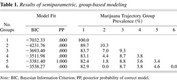
Results of semiparametric, group-based modeling
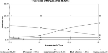
The trajectories of marijuana use.
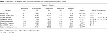
One-way ANOVAs for Time 1 adolescent behaviors by marijuana trajectory group
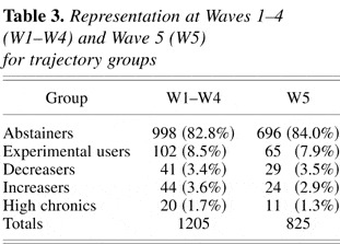
Representation at Waves 1–4 (W1–W4) and Wave 5 (W5) for trajectory groups
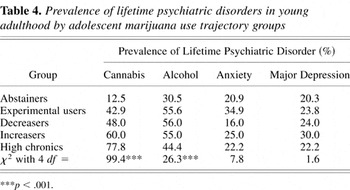
Prevalence of lifetime psychiatric disorders in young adulthood by adolescent marijuana use trajectory groups
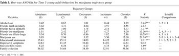
One-way ANOVAs for Time 5 young adult behaviors by marijuana trajectory group
 You have
Access
- 225
- Cited by