1. Introduction
Despite 130 years of research efforts since the seminal work of Reynolds (Reference Reynolds1883), a thorough comprehension of the mechanism of transition from ordered to chaotic behaviour in shear flows has not yet been achieved. Indeed, even very simple shear flows, such as flow in a pipe or flow driven by two parallel moving flat plates (plane Couette flow, or pCf), show very complex behaviours (Eckhardt et al. Reference Eckhardt, Schneider, Hof and Westerweel2007). As a result of the analysis of perturbation lifetimes (see Schmiegel & Eckhardt Reference Schmiegel and Eckhardt1997; Hof et al. Reference Hof, Westerweel, Schneider and Eckhardt2006; Schneider et al. Reference Schneider, De Lillo, Buehrle, Eckhardt, Dörnemann, Dörnemann and Freisleben2010), it has been observed that sustained turbulence does not exist for sufficiently small flow domains. In fact, turbulence has been shown to be transient, and lifetimes of turbulent trajectories are distributed exponentially with the Reynolds number (Dauchot & Daviaud Reference Dauchot and Daviaud1995; Bottin & Chaté Reference Bottin and Chaté1998; Bottin et al. Reference Bottin, Daviaud, Manneville and Dauchot1998). Moreover, recent analysis of experimental data (Hof et al. Reference Hof, Westerweel, Schneider and Eckhardt2006) and numerical simulations (Schneider et al. Reference Schneider, De Lillo, Buehrle, Eckhardt, Dörnemann, Dörnemann and Freisleben2010) have shown that lifetimes increase with the Reynolds number without diverging. Therefore, a critical Reynolds number, above which a persistent turbulent state could be achieved, would not exist. On the other hand, in large domains a critical Reynolds number for sustained turbulence may appear. In fact, as shown by Avila et al. (Reference Avila, Moxey, de Lozar, Avila, Barkley and Hof2011) for pipe flow, persistent turbulence can be achieved by the spatial coupling of transiently chaotic flow regions rather than by an increase in temporal complexity.
In both cases, whether turbulence is sustained or not, for values of the Reynolds number above a certain threshold (moreover, only approximately known), finite-energy perturbations of a certain shape can trigger transition to a chaotic dynamics. How these critical parameters for transition depend on each other is very intriguing and difficult to determine accurately.
For the case of plane Couette flow, of interest here, Romanov (Reference Romanov1973) is credited with demonstrating that laminar flow is linearly stable, and therefore the onset of a chaotic state cannot be connected to the linear amplification of an infinitesimal perturbation of the laminar velocity profile. For most values of the Reynolds number and of the size of the domain, the laminar state (LS) is the only stable fixed point in the state space. In the present work, a small domain has been considered, for which a saddle node bifurcation appears at a given Reynolds number (Kreilos & Eckhardt Reference Kreilos and Eckhardt2012). At the bifurcation point, the upper branch (UB) state is stable and the lower branch (LB) has only one unstable direction (Nagata Reference Nagata1990; Waleffe Reference Waleffe2003; Wang, Gibson & Waleffe Reference Wang, Gibson and Waleffe2007). Increasing the Reynolds number beyond a certain threshold
 $\mathit{Re}_{UB}$
, the UB experiences secondary bifurcations leading to a disordered trajectory in the state space, whereas the LB maintains a single unstable direction only (Schneider et al.
Reference Schneider, Gibson, Lagha, De Lillo and Eckhardt2008).
Studying the time evolution of the perturbations of the LS at Reynolds numbers larger than
 $\mathit{Re}_{UB}$
, it has been found that (almost) all trajectories in the state space end up at the stable fixed point: some of them relax smoothly, whereas others follow a fairly long (i.e. long lifetime) disordered route and may eventually escape towards the laminar attractor. In the state space spanned by the instantaneous three-dimensional velocity field, these two types of perturbations are separated by a codimension-one hypersurface, known as the edge of chaos (Ott Reference Ott2002; Schneider & Eckhardt Reference Schneider and Eckhardt2006; Skufca, Yorke & Eckhardt Reference Skufca, Yorke and Eckhardt2006). This hypersurface generalizes the basin boundary of the LS to the case of non-persistent turbulence (Vollmer, Schneider & Eckhardt Reference Vollmer, Schneider and Eckhardt2009), since it separates the LS from a chaotic saddle with a constant probability of decay (Schneider et al.
Reference Schneider, De Lillo, Buehrle, Eckhardt, Dörnemann, Dörnemann and Freisleben2010). The trajectories evolving on the edge of chaos are attracted towards one or more relative attractors (Itano & Toh Reference Itano and Toh2001), known as edge states, which are invariant solutions of the Navier–Stokes equations with a single unstable direction. At moderate Reynolds numbers, the stable manifold of the LB state coincides with the edge of chaos and the LB state is the edge state itself (Wang et al.
Reference Wang, Gibson and Waleffe2007; Schneider et al.
Reference Schneider, Gibson, Lagha, De Lillo and Eckhardt2008). Thus, the stable manifold of the LB state divides the state space into two regions: initial conditions from one side decay smoothly to the laminar profile; initial conditions on the other side flow through a disordered dynamics and eventually decay towards the laminar state. However, it is still not clear how the latter trajectories pass from the chaotic to the laminar side when the decay occurs, since they cannot intersect the invariant manifold representing the edge. Recently, the study of the decaying trajectories from the chaotic saddle to the LS has led to the conjecture that the edge is wrapped around the chaotic saddle, allowing the ‘unfolding’ of the chaotic trajectories back to the LS (Lebovitz & Mariotti Reference Lebovitz and Mariotti2013; Chantry & Schneider Reference Chantry and Schneider2014). This feature of the edge of chaos for plane Couette flow has an important consequence for the dynamics of perturbations lying close to the folds of the edge of chaos: in fact, slightly increasing the amplitude of a given perturbation triggering turbulence may lead to relaminarization, or, in the same way, decreasing the amplitude of a relaminarizing perturbation may lead to a chaotic dynamics (Chantry & Schneider Reference Chantry and Schneider2014). Thanks to very accurate control of the perturbations, somewhat similar behaviour has been found by Tasaka, Schneider & Mullin (Reference Tasaka, Schneider and Mullin2010) for pipe flow, although the geometry of the state space is different. In particular, the authors showed that, close to a ‘critical’ perturbation amplitude, folds are present in the laminar–turbulent boundary of such a flow. Thus, for these types of shear flows, the problem of determining the threshold energy to trigger subcritical transition consists in finding the states on this complex hypersurface with minimal distance (in the energy norm) from the laminar state.
Investigating the threshold amplitude or energy for inducing subcritical transition in shear flows has been the object of many studies: the first attempt of Reddy et al. (Reference Reddy, Schmid, Baggett and Henningson1998), who provided a neutral curve for streak instability using linear stability analysis; the study of the lower bounds for transition performed by Cossu (Reference Cossu2005) using the low-dimensional model based on the Galerkin projection of Waleffe (Reference Waleffe1997); the investigation of minimal-energy perturbations inducing transition using a combination of a finite number of linear optimal modes by Duguet, Brandt & Larsson (Reference Duguet, Brandt and Larsson2010). Very recently, more thorough attempts have been made to search for the perturbations of minimal energy triggering transition for pipe (Pringle & Kerswell Reference Pringle and Kerswell2010; Pringle, Willis & Kerswell Reference Pringle, Willis and Kerswell2012), boundary layer (Cherubini et al.
Reference Cherubini, De Palma, Robinet and Bottaro2010a
, Reference Cherubini, De Palma, Robinet and Bottaro2011) and Couette flow (Monokrousos et al.
Reference Monokrousos, Bottaro, Brandt, Di Vita and Henningson2011; Rabin, Caulfield & Kerswell Reference Rabin, Caulfield and Kerswell2012; Cherubini & De Palma Reference Cherubini and De Palma2013; Duguet et al.
Reference Duguet, Monokrousos, Brandt and Henningson2013). To determine the initial condition of minimal energy leading eventually to transition, these authors optimize at a large target time a functional linked to the turbulent dynamics, the perturbation kinetic energy (see Pringle & Kerswell Reference Pringle and Kerswell2010, Cherubini et al.
Reference Cherubini, De Palma, Robinet and Bottaro2011, Pringle et al.
Reference Pringle, Willis and Kerswell2012, Rabin et al.
Reference Rabin, Caulfield and Kerswell2012, Cherubini & De Palma Reference Cherubini and De Palma2013, Duguet et al.
Reference Duguet, Monokrousos, Brandt and Henningson2013) or the time-averaged dissipation (see Monokrousos et al.
Reference Monokrousos, Bottaro, Brandt, Di Vita and Henningson2011). They then bisect the initial energy of such a ‘nonlinear optimal perturbation’ (NLOP) until it approaches the edge of chaos. Using this approach, one can find the perturbation of minimal energy
 $E_{c}$
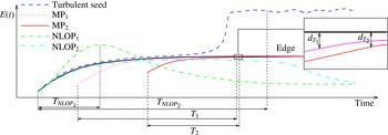
, which brings the flow asymptotically close to the edge state. Such a perturbation has been called a ‘minimal seed’ by Pringle & Kerswell (Reference Pringle and Kerswell2010). The time evolution of the energy of this perturbation is represented in figure 1 by the solid black line. The initial perturbation, having initial energy
 $E_{c}$
, evolves asymptotically towards the edge state (assumed here to be steady and thus characterized by a constant energy), whereas a perturbation having the same shape and an infinitesimally higher energy
 $E_{c}+{\it\epsilon}$
, whose time evolution is represented by the dashed line, leads to chaotic behaviour in a long time, namely, it will be a ‘turbulent seed’. Since convergence of the optimization to a turbulent state cannot be achieved (Rabin et al.
Reference Rabin, Caulfield and Kerswell2012), the minimal seed can be found by computing the NLOP for a long target time and an initial energy lower than
 $E_{c}$
, and then bisecting this initial energy until it reaches the vicinity of the edge state (within a tolerance
 ${\it\epsilon}$
). The dot-dashed and dot-dot-dashed lines in figure 1 show the energy evolution of two NLOPs, computed for an initial energy slightly lower than
 $E_{c}$
, for a short (
 $T_{NLOP_{1}}$
) and a large (
 $T_{NLOP_{2}}$
) target time, respectively. The sketch in figure 1 shows that, even if the former reaches a larger energy gain at the target time, only the latter approaches the minimal seed and gets close to the edge state. In fact, as explained by Rabin et al. (Reference Rabin, Caulfield and Kerswell2012), different solution branches obtained by the optimization (nonlinear or quasi-linear branches) may ‘mask’ the minimal seed, unless sufficiently long optimization intervals, and initial energies sufficiently close to the critical energy, are chosen. Rabin et al. (Reference Rabin, Caulfield and Kerswell2012) have shown that perturbations achieving an optimal energy gain at a short/intermediate target time may eventually decay to the laminar state. In fact, optimizing the energy for small target times does not allow nonlinear effects to kick in, since they may not have the time to be triggered if the initial perturbation has an initial energy close to the threshold
 $E_{c}$
. As a result, the optimization algorithm will probably converge to a quasi-linear or weakly nonlinear optimal; these perturbations are able to achieve a very large and rapid energy growth through linear transient growth mechanisms, but they will not lead in the vicinity of the edge state, which needs nonlinear effects to be sustained. Thus, the algorithm used in previous studies to find the minimal seed does not allow one to compute perturbations of minimal energy approaching the edge state in a ‘short’ time (within a prescribed distance
 $d_{T}$
). These perturbations will thereafter be called minimal perturbations (
 $\text{MP}_{1}$
and
 $\text{MP}_{2}$
), and they represent the focus of this work. The solid red and dotted magenta lines in figure 1 sketch the time evolution of the energy of two minimal perturbations approaching the edge state at two different short target times (
 $T_{1}$
and
 $T_{2}$
) with minimal initial energy. The inset shows the distance
 ${d_{T}}_{1}$
and
 ${d_{T}}_{2}$
reached at the target time from the edge state. Since the laminar–turbulent boundary appears to be fractal (Lebovitz Reference Lebovitz2009; Vollmer et al.
Reference Vollmer, Schneider and Eckhardt2009; Lai & Tél Reference Lai and Tél2011), folded and probably wrapped around the chaotic saddle (Lebovitz & Mariotti Reference Lebovitz and Mariotti2013; Chantry & Schneider Reference Chantry and Schneider2014), it is possible that many local energy minima populate the folds of the edge of chaos. In fact, it has been observed that two initial perturbations having a slightly different initial energy may result in very different outcomes in terms of transition probabilities (Tasaka et al.
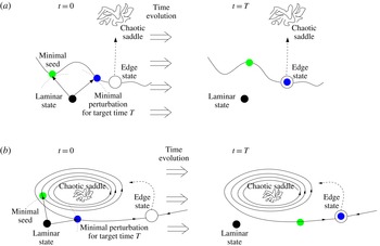
Reference Tasaka, Schneider and Mullin2010; Chantry & Schneider Reference Chantry and Schneider2014). Therefore, the analysis of the structure of the edge of chaos and its local minimal-energy states is interesting when deepening our understanding of the subcritical transition process at least for the simple case of plane Couette flow, for which the edge state is steady (equilibrium point). This can be done by determining the minimal perturbations approaching the edge state in a short time, having an initial energy (larger but) comparable to that of the ‘asymptotic’ minimal seed. One of these perturbations is represented by the blue dot in figure 2, where two different views of the edge of chaos are sketched, namely, a local view of a fold (figure 2
a) and a global view of the edge of chaos wrapped around the chaotic saddle (figure 2
b). In both sketches, the black circle is the laminar fixed point, and the white dot denotes the relative attractor on the edge of chaos, whereas the scattered trajectory represents the chaotic saddle. The stable and unstable manifolds of the edge state are indicated by the solid and dashed lines, respectively. In the former, one can determine the states of minimal distance from the laminar state (blue circle in the left-hand part of the figure), approaching the edge state at a given target time (blue circle in the right-hand part). Some states of even lower energy could exist on the stable manifold (green circle in the left-hand part, representing the minimal seed), but they would approach the relative attractor in a larger time interval (green circle in the right-hand part). It is noteworthy that minimal perturbations approaching the edge state in a small time can be responsible for a sudden transition of the flow from the laminar state to turbulence and could be the key to a shear-flow control strategy based on the stabilization of unstable states with low dissipation rate, such as the edge state, exploiting the sensitivity of the system to small disturbances (Pyragas Reference Pyragas1992). An example of how it is possible to increase the threshold energy
 $E_{c}$
by using a variational approach has recently been provided by Rabin, Caulfield & Kerswell (Reference Rabin, Caulfield and Kerswell2014).
Sketch of the time evolution of the energy for different initial perturbations of the laminar state. The dot-dashed and dot-dot-dashed lines represent the evolution of two NLOPs, optimizing the energy gain at a small and a large target time,
 $T_{NLOP_{1}}$
and
 $T_{NLOP_{2}}$
, respectively, both computed for an initial energy
 $E_{c}-{\it\epsilon}$
. The first one induces a larger energy gain than the second one, but only the latter approaches the minimal seed as
 ${\it\epsilon}\rightarrow 0$
. The turbulent seed for
 ${T_{NLOP}}_{2}$
and initial energy
 $E_{c}+{\it\epsilon}$
is plotted by the dashed line, whereas the evolution of the minimal seed with initial energy
 $E_{c}$
towards the edge state is provided by the solid thick black line. The solid red and dotted magenta lines represent the minimal perturbations (
 $\text{MP}_{1}$
,
 $\text{MP}_{2}$
) approaching the edge at a finite time, for two different (small) target times
 $T_{1}$
and
 $T_{2}$
. The inset shows the distance
 $d_{T}$
from the edge (in the energy norm) at the target time, for the two different minimal perturbations.

Sketch of the problem on an energy-normed projection of the state space, considering two different views of the edge of chaos: a local view of a fold (a) and a global view of the edge of chaos wrapped around the chaotic saddle (b). The black circle is the laminar fixed point; the white dot denotes the relative attractor on the edge of chaos; the scattered trajectory on the top represents the chaotic saddle. The stable and unstable manifolds of the edge state are indicated by the solid and dashed lines, respectively. On the former, one can determine the states of minimal distance from the laminar state, approaching the edge state at a given target time (blue circle). Some states of even lower energy could exist on the stable manifold, but they would approach the relative attractor at a larger time (green circle).

In conclusion, the aim of this work is to find local minimal-energy states lying close to the laminar–turbulent boundary, requiring a given time to approach the edge state within a tolerance level. For this purpose, we use a Lagrange multiplier method to minimize the initial energy of the perturbations while limiting to a small value the distance from the edge state at a given target time. We find that by increasing the target time, the minimal initial energy decreases following a power law. Finally, for large target times, it reaches a constant value close to the energy of the minimal seed computed using the technique of Rabin et al. (Reference Rabin, Caulfield and Kerswell2012).
The structure of the paper is as follows. The problem set-up and the numerical technique are described in § 2. The results of the minimization procedure are presented in § 3, where the energy, shape, and dynamics of the minimal perturbations are analysed. The main conclusions are given in § 4.
2. Problem set-up
We consider the case of incompressible flow between two counter-sliding plates, known as plane Couette flow (pCf). Non-dimensional variables are chosen such that half the distance between the plates is
 $h=1$
and the velocity of the plates is
 $U_{w}=\pm 1$
. The dynamics of such a flow is described by the following Navier–Stokes equations:
 $$\begin{eqnarray}\displaystyle & \displaystyle \frac{\partial \boldsymbol{U}}{\partial t}+(\boldsymbol{U}\boldsymbol{\cdot }\boldsymbol{{\rm\nabla}})\boldsymbol{U}=-\boldsymbol{{\rm\nabla}}P+\frac{1}{\mathit{Re}}{\rm\nabla}^{2}\boldsymbol{U}, & \displaystyle\end{eqnarray}$$
 $$\begin{eqnarray}\displaystyle & \displaystyle \boldsymbol{{\rm\nabla}}\boldsymbol{\cdot }\boldsymbol{U}=0, & \displaystyle\end{eqnarray}$$
 $\boldsymbol{U}$
is the velocity vector,
 $P$
is the pressure term, and
 $\mathit{Re}$
is the Reynolds number. The laminar flow in the (sliding)
 $x$
direction between the plates has a linear profile,
 $$\begin{eqnarray}U(y)=y,\end{eqnarray}$$
where
 $y$
is the wall-normal direction, whereas the spanwise direction will be referred to as
 $z$
. A small computational box with dimensions
 $L_{x}\times L_{y}\times L_{z}=4{\rm\pi}\times 2\times 2{\rm\pi}$
is considered, which is the same as that used by Schneider et al. (Reference Schneider, Gibson, Lagha, De Lillo and Eckhardt2008) for the computation of the edge state, and by Monokrousos et al. (Reference Monokrousos, Bottaro, Brandt, Di Vita and Henningson2011) for the computation of the minimal seed. The Navier–Stokes equations are discretized employing a
 $201\times 100\times 61$
grid and solved using a finite-difference fractional-step method with second-order accuracy in space and time (Verzicco & Orlandi Reference Verzicco and Orlandi1996). At the walls, a no-slip boundary condition is prescribed (
 $U(y=\pm 1)=\pm 1$
), whereas in the spanwise and streamwise direction periodicity is imposed for the three velocity components and the pressure. The code has been validated by computing, via an edge-tracking procedure, the steady LB state of Schneider et al. (Reference Schneider, Gibson, Lagha, De Lillo and Eckhardt2008), at
 $\mathit{Re}=400$
. This solution is characterized by a bent streaky structure flanked by streamwise vortices, with a finite-translation symmetry in the spanwise direction, and a shift-reflection symmetry in the streamwise direction (solution type
 $EQ_{1}$
in Gibson, Halcrow & Cvitanović Reference Gibson, Halcrow and Cvitanović2009).
2.1. Minimization method
In this work we aim to find the perturbations of minimal energy placed very close to the edge of chaos and approaching its relative attractor in a given (small) time. Such perturbations must be confined in the neighbourhood of the stable manifold of the edge state, which, in the case under consideration, is the steady LB state of Schneider et al. (Reference Schneider, Gibson, Lagha, De Lillo and Eckhardt2008), a version of the first invariant exact solution identified by Nagata (Reference Nagata1990) in plane Couette flow. Notice that the problem considered is a two-time-level optimization: in fact we require the solution to satisfy at the target time a constraint on the distance of the perturbation from the edge state, while minimizing the energy at the initial time. We propose a possible procedure to achieve this goal, based on a particular choice of the objective function and imposing an upper-bound value for the distance
 $d_{T}$
at the target time, as explained in the following.
Let us consider a perturbation
 $(\boldsymbol{u},p)$
to the laminar state, where
 $\boldsymbol{u}=(u,v,w)^{\text{T}}$
is the perturbation velocity vector and
 $p$
is the pressure perturbation. We define the scalar product as
 $$\begin{eqnarray}\left\langle \boldsymbol{u},\boldsymbol{v}\right\rangle =\frac{1}{V}\int _{V}\boldsymbol{u}\boldsymbol{\cdot }\boldsymbol{v}\text{d}V,\end{eqnarray}$$
where
 $V$
indicates the volume of the computational domain. The perturbation energy at initial time
 $t=0$
is thus computed as
 $$\begin{eqnarray}E_{0}={\textstyle \frac{1}{2}}\langle \boldsymbol{u}_{0},\boldsymbol{u}_{0}\rangle ,\end{eqnarray}$$
where
 $\boldsymbol{u}_{0}$
is the initial perturbation of the laminar state. This initial perturbation would evolve in time achieving, at an assigned target time
 $T$
, a distance from the edge state
 $\boldsymbol{u}_{ES}$
, which we want to keep small. The distance is defined as
 $$\begin{eqnarray}d_{T}=\frac{\left\langle (\boldsymbol{u}(T)-\boldsymbol{u}_{ES}),(\boldsymbol{u}(T)-\boldsymbol{u}_{ES})\right\rangle }{\left\langle \boldsymbol{u}_{ES},\boldsymbol{u}_{ES}\right\rangle },\end{eqnarray}$$
where also the edge state has been expressed as a perturbation of the laminar state, the term at the denominator being a normalization with respect to the edge-state energy.
In order to minimize the initial perturbation energy and to limit to a small value the distance from the edge at a time
 $T$
, we define the objective function for the Lagrange minimization procedure as
 $$\begin{eqnarray}\Im =d_{T}E_{0}.\end{eqnarray}$$
It is necessary to include the distance
 $d_{T}$
in the objective function; otherwise, during the minimization procedure of
 $E_{0}$
, the algorithm would immediately lead the perturbation far from the edge of chaos. Thus, to limit the value of
 $d_{T}$
we choose to include it in the objective function, and constrain its value under a given threshold. As discussed below, since the distance tends to a constant value at convergence (its gradient becoming very small), and since the gradient of the objective function is equivalent to
 $$\begin{eqnarray}\boldsymbol{{\rm\nabla}}_{\boldsymbol{u}_{0}}\Im =d_{T}\boldsymbol{{\rm\nabla}}_{\boldsymbol{u}_{0}}E_{0}+E_{0}\boldsymbol{{\rm\nabla}}_{\boldsymbol{u}_{0}}d_{T},\end{eqnarray}$$
the algorithm will indeed converge to a minimum value of
 $E_{0}$
. It is noteworthy that different choices of the function
 $\Im (E_{0},T)$
could have been used, leading to different expressions of the gradient. For instance, we have also tested the objective function
 $\Im =E_{0}+{\it\gamma}d_{T}$
. However, for this particular form of
 $\Im$
we have found the convergence very sensitive to the choice of the cost parameter
 ${\it\gamma}$
. Thus, only the objective function provided in (2.7) has been considered for our minimizations. Finally, note that the distance metric (2.6) assumes a specific phase for the edge; nevertheless, the results of the optimization are not affected by this choice. In fact, we have verified that the minimal perturbation computed with a given phase satisfies the minimum energy condition for an arbitrary variation of the phase.
The chosen objective function is minimized over all of the perturbations verifying the incompressible Navier–Stokes (NS) equations. These equations are imposed as constraints by means of the Lagrange multipliers
 $(\boldsymbol{u}^{\dagger },p^{\dagger })$
, so the functional to be minimized is
 $$\begin{eqnarray}\mathscr{L}=\Im -\int _{0}^{T}\{\langle \boldsymbol{u}^{\dagger },NS(\boldsymbol{u},p)\rangle +\langle p^{\dagger },\boldsymbol{{\rm\nabla}}\boldsymbol{\cdot }\boldsymbol{u}\rangle \}\text{d}t.\end{eqnarray}$$
In order to find the minimum of the functional, its first variation with respect to all of the variables must be set to zero. In particular, zeroing the first variation of the functional with respect to the direct and adjoint variables (the Lagrange multipliers) provides the adjoint and the direct equations, respectively, as well as the compatibility conditions which provide a relation between direct and adjoint variables at
 $t=T$
. The gradient
 $\boldsymbol{{\rm\nabla}}_{\boldsymbol{u}_{0}}\mathscr{L}$
, having the form
 $$\begin{eqnarray}\displaystyle \left.\begin{array}{@{}l@{}}\displaystyle \frac{\partial \mathscr{L}}{\partial u_{0}}=-2u_{0}d_{T}+u^{\dagger }(0),\\ \displaystyle \frac{\partial \mathscr{L}}{\partial v_{0}}=-2v_{0}d_{T}+v^{\dagger }(0),\\ \displaystyle \frac{\partial \mathscr{L}}{\partial w_{0}}=-2w_{0}d_{T}+w^{\dagger }(0),\end{array}\right\} & & \displaystyle\end{eqnarray}$$
is iteratively minimized by using a conjugate gradient procedure based on the forward and backward time integration of the direct and adjoint systems (Cherubini et al.
Reference Cherubini, De Palma, Robinet and Bottaro2010a
). At the first iteration, the initial state is updated in the steepest descent direction with an adjustable step length
 ${\it\alpha}$
, so that
 $\boldsymbol{u}_{0}^{(n+1)}=\boldsymbol{u}_{0}^{n}-{\it\alpha}^{n}{\boldsymbol{{\rm\nabla}}_{\boldsymbol{u}_{0}}\mathscr{L}}^{n}$
. After the first iteration, the successive steps are taken along a conjugate direction,
 ${\it\Lambda}\boldsymbol{u}_{0}$
, which is computed on the basis of the gradient at two consecutive iterations according to
 ${\it\Lambda}\boldsymbol{u}_{0}^{(n+1)}={\boldsymbol{{\rm\nabla}}_{\boldsymbol{u}_{0}}\mathscr{L}}^{(n+1)}+{\it\beta}^{(n+1)}{\it\Lambda}\boldsymbol{u}_{0}^{n}$
.
Moreover, since we want to minimize
 $E_{0}$
while limiting the distance from the edge state at the target time to a given value
 ${\it\epsilon}_{T}$
, we add a constraint to the procedure: we start the minimization procedure from the edge state itself and require that
 $d_{T}\leqslant {\it\epsilon}_{T}$
, with
 ${\it\epsilon}_{T}=10^{-5}$
, which represents the maximum level of tolerance for the final convergence. When such a threshold is overtaken, the iterations are repeated keeping the initial energy fixed to the value of the previous iteration, but employing smaller steps in the direction opposed to the conjugate gradient until
 $d_{T}$
decreases to a value smaller than
 ${\it\epsilon}_{T}$
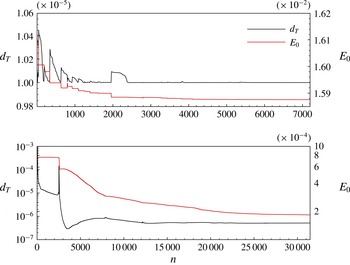
. Figure 3(a,b) shows the convergence histories of
 $E_{0}$
and
 $d_{T}$
for two minimizations performed for
 $T=5$
and
 $T=60$
, respectively. Both figures show that in the initial phase of the procedure, the algorithm tends to minimize
 $d_{T}$
(maintaining
 $E_{0}$
constant) to bring its value below the chosen threshold
 ${\it\epsilon}_{T}$
. When
 $d_{T}<{\it\epsilon}_{T}$
,
 $E_{0}$
starts decreasing, until the threshold is overtaken once again, and
 $d_{T}$
is again decreased below the chosen threshold. The convergence histories provided in figure 3 show that this procedure is substantially equivalent to a sequential minimization of
 $E_{0}$
and
 $d_{T}$
. In fact, this procedure always leads, at the end of the minimization procedure, to a value of
 $d_{T}$
which is constant and smaller than
 ${\it\epsilon}_{T}$
. Therefore, since towards convergence
 $\boldsymbol{{\rm\nabla}}_{\boldsymbol{u}_{0}}d_{T}\approx 0$
, the gradient of the objective function defined in (2.8) almost coincides with the gradient of
 $E_{0}$
, which is indeed minimized. This can be explained by considering that the edge state is a relative attractor for the perturbations lying on the edge of chaos; therefore, if we limit the distance of the perturbation from the edge state at target time, we constrain it to remain close to the edge of chaos at the initial time within a given level of accuracy.
Minimal initial energy
 $E_{0}$
and distance from the edge versus number of iterations for the minimization at
 $T=5$
(a) and
 $T=60$
(b).

The minimization procedure for a chosen target time
 $T$
can be thus summarized as follows.
-
(i) The initial guess for the solution at
 $t=0$
,
$\boldsymbol{u}_{0}$
, is provided.
-
(ii) The Navier–Stokes equations (direct problem) are solved up to
$t=T$
. -
(iii) The distance from the edge,
$d_{T}$
, is evaluated at time
$T$
.-
(a) If
$d_{T}<{\it\epsilon}_{T}$
, the procedure continues from step (iv). -
(b) If
$d_{T}>{\it\epsilon}_{T}$
,
$\boldsymbol{u}_{0}$
is updated in the opposite direction to the conjugate gradient (computed at the previous iteration) with halved step length
${\it\alpha}/2$
and fixed initial energy
$E_{0}$
. The procedure continues from step (ii).
-
-
(iv) The adjoint variables,
$(\boldsymbol{u}^{\dagger }(T),p^{\dagger }(T))$
, are computed using the compatibility conditions. -
(v) The adjoint problem is integrated backward in time from
$t=T$
to
$t=0$
. -
(vi) The gradient
$\boldsymbol{{\rm\nabla}}_{\boldsymbol{u}_{0}}\mathscr{L}$
is evaluated at
$t=0$
.-
(a) If
$\boldsymbol{{\rm\nabla}}_{\boldsymbol{u}_{0}}\mathscr{L}$
is smaller than the chosen threshold, the loop is stopped. -
(b) If
$\boldsymbol{{\rm\nabla}}_{\boldsymbol{u}_{0}}\mathscr{L}$
is larger than the threshold,
$\boldsymbol{u}_{0}$
is updated in the opposite direction to the conjugate gradient with step length
${\it\alpha}$
. The procedure continues from step (ii).
-


We have verified that for
 ${\it\epsilon}_{T}<10^{-5}$
the shape of the minimal perturbations is only slightly dependent on the value of
 $d_{T}$
achieved at convergence. This is expected since, due to the sensitivity of the problem to initial conditions, when the target time is finite, a variation of order
 ${\it\epsilon}_{T}$
of the value of
 $d_{T}$
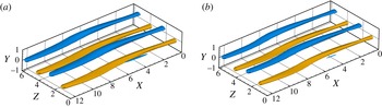
would result from a variation of the initial energy value of a lower order of magnitude, resulting in negligible modifications of the initial perturbation. For example, figure 4 shows that even at the lowest target time considered here,
 $T=5$
, changing the value of
 ${\it\epsilon}_{T}$
from
 $10^{-5}$
to
 $10^{-8}$
affects the shape of the perturbation only in a negligible way. It is also worth noticing that particular care is needed in the choice of the initial guess. In fact, even though the distance from the edge is included in the functional to be minimized, small changes of the initial perturbation can drive the trajectory far from the edge of chaos. Thus, to keep the perturbation on the laminar–turbulent boundary, we usually take the edge state itself as the initial guess for the minimizations. Starting from this initial guess, the initial perturbation is updated by a very small amount at each iteration, so that up to 40 000 iterations are needed to achieve convergence at a given target time, making the problem very computationally expensive.
Isosurfaces of the streamwise velocity perturbation (
 $u=\pm 0.3$
, light blue and yellow for the negative and positive value, respectively) of the minimal perturbation obtained for
 $T=5$
and for a distance from the edge limited to (a)
 ${\it\epsilon}_{T}=10^{-5}$
and (b)
 ${\it\epsilon}_{T}=10^{-8}$
.

3. Results
3.1. Minimal perturbations approaching the edge
Minimal perturbations approaching the edge state at
 $\mathit{Re}=400$
have been computed for seven target times,
 $T=5$
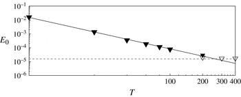
, 20, 40, 60, 80, 100, 200. Figure 5 shows the value of the minimal energy
 $E_{min}$
versus the target time
 $T$
in the range
 $5\leqslant T\leqslant 400$
. The values of
 $E_{min}$
in the range
 $5\leqslant T\leqslant 200$
have been computed by the minimization method described above (black triangles); for
 $T_{NLOP}=200,300,400$
(white triangles), the bisection method of Rabin et al. (Reference Rabin, Caulfield and Kerswell2012), with only two-digit accuracy, has been employed to extend the analysis towards the asymptotic minimal seed. It is worth observing that different values of
 $T_{NLOP}<200$
have been tested too, but the computed optimal perturbations did not directly approach the edge state, since they induced bursting phenomena characterized by large kinetic energy growth (see the discussion in § 1 about the ‘masking’ of the minimal seed by different optimal branches at small target time). Plotting the values of
 $E_{min}$
on a double logarithmic scale, a linear slope is recovered for
 $T\leqslant 200$
. Thus, it appears that, for small target times,
 $E_{min}$
varies with
 $T$
following a power law whose best fit is given by
 $E_{min}\propto T^{-1.75}$
. It is worth noticing that the NLOP obtained by the bisection method for
 $T_{NLOP}=200$
is very close to the minimal perturbation obtained for the same target time by the minimization method, further validating these results. Nonetheless, a small difference (of order
 $10^{-6}$
) can be observed in the minimal energy obtained using these two different methods. This difference very likely depends on the different distance from the edge state that is reached at target time by the two disturbances. In fact, the minimal perturbation reaches the proximity of the edge state within a distance smaller than
 ${\it\epsilon}_{T}=10^{-5}$
, whereas the NLOP has been computed with only two-digit accuracy, allowing perturbations of slightly lower energy to approach the edge state within this larger tolerance. Despite this small difference, both perturbations fall very close to the power law curve. On the other hand, for
 $T_{NLOP}>200$
the value of the minimal energy deviates from the power law and appears to reach a constant value approximating the energy of the minimal seed
 $E_{c}$
within a small tolerance. In fact, since the flow is linearly stable, it can be anticipated that the power law achieved for small target times cannot hold at large ones, since for
 $T\rightarrow \infty$
there should exist a finite minimum value of the energy to trigger transition. This value corresponds to the energy of the minimal seed, which, in the present case, appears to be close to
 $E_{c}=1.701\times 10^{-5}$
. This critical value matches pretty well with the value extrapolated from the results obtained by Duguet et al. (Reference Duguet, Monokrousos, Brandt and Henningson2013), who have found that the critical energy
 $E_{c}$
in a Couette flow varies with the Reynolds number as
 $\mathit{Re}^{-2.7}$
. The minimal energy values
 $E_{min}$
, together with the power law holding for
 $5\leqslant T\leqslant 200$
, allow one to establish a threshold for the initial energy needed to approach the edge state at a given target time in plane Couette flow. Thus, the present results guarantee that perturbations of energy
 $E<E_{min}$
cannot reach chaos at a time
 $t<T$
(with the limiting case for
 $T\rightarrow \infty$
, where
 $E_{min}=E_{c}$
).
Minimal perturbation energy versus target time in a double logarithmic scale. The black triangles are the results of the minimization procedure; the white ones correspond to the NLOPs with bisected initial energy. The solid line represents the most accurate power fit; the dashed line indicates the minimal seed energy (Rabin et al. Reference Rabin, Caulfield and Kerswell2012; Duguet et al. Reference Duguet, Monokrousos, Brandt and Henningson2013).

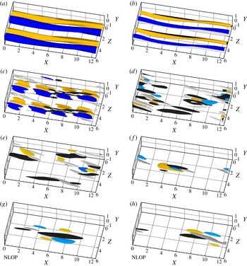
Structure of the edge state (a) and of the minimal perturbations approaching it at target time (b)
 $T=5$
, (c)
 $T=20$
, (d)
 $T=60$
, (e)
 $T=80$
, and ( f)
 $T=100$
. The NLOPs obtained by energy optimization and bisection with target time
 $T=200,300$
are shown in (g,h), respectively. The white and black surfaces represent the positive and negative streamwise component of the vorticity perturbation: (a–h)
 ${\it\omega}_{x}=\pm (1.7,1.7,0.9,0.4,0.37,0.18,0.17,0.17)$
. Yellow and blue represent the positive and negative streamwise velocity component: (a–h)
 $u=\pm (0.3,0.3,0.08,0.045,0.035,0.17,0.2,0.2)$
.

The edge state is shown in figure 6(a), and the structures of the minimal perturbations are given in figure 6(b–f), for
 $T=5,20,60,80,100$
, respectively; furthermore, the NLOPs for
 $T_{NLOP}=200,300$
are shown in figure 6(g,h), respectively. For the smallest target time,
 $T=5$
, the minimal perturbation is very close to the edge state, preserving the symmetries that characterize the LB state. For
 $T=20$
, the shift-reflection symmetry is broken, but the perturbation is still invariant with respect to a finite translation in the spanwise direction. Moreover, the streamwise perturbation velocity (blue and yellow for negative and positive values) begins to be more localized in the streamwise direction, showing alternated patches instead of streaky structures. For
 $T\geqslant 40$
, the spanwise translation symmetry is also broken, and the perturbation begins to localize in the streamwise direction too. In particular, a repeated basic structure can be identified, which is characterized by scattered patches of streamwise velocity with inclined streamwise vortices (black and white) on their flanks. Further increasing the target time, a stronger localization in both the streamwise and spanwise directions is observed, as shown in figure 6( f) for
 $T=100$
. It is interesting that the shape of the minimal perturbation remains characterized by a similar basic structure, which strongly recalls the minimal seed of turbulent transition found by Monokrousos et al. (Reference Monokrousos, Bottaro, Brandt, Di Vita and Henningson2011), Rabin et al. (Reference Rabin, Caulfield and Kerswell2012) and Cherubini & De Palma (Reference Cherubini and De Palma2013) for plane Couette flow. In fact, comparing the lower frames of figure 6, one can verify that the shape of the minimal perturbation at
 $T=100$
tends to resemble the shape of the NLOP found at large target times for an initial energy close to
 $E_{c}$
. This indicates that, for sufficiently large target times, the minimal perturbations on the edge of chaos approach the minimal seed, but they largely differ from it at short times. In particular, it seems that minimal perturbations need at least a time of the order of 100 for unpacking from a localized structure and approaching the edge state. When a smaller time is given to the perturbation for approaching the edge (
 $20<T<100$
), the disturbance cannot localize too much while at the same time keeping the initial energy at a minimum. Thus, the perturbation unpacks in several patches having a structure similar to that of the minimal seed, which is the most efficient for inducing transition in terms of energy.
It is also noteworthy that, for all of the values of
 $T$
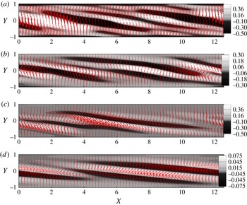
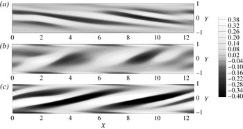
, the minimal perturbations are characterized by vortical structures inclined in the opposite direction with respect to that of the base flow. This is clearly observed in figure 7, where the streamwise vorticity perturbations are shown on a
 $z={\rm\pi}$
plane, for the minimal perturbations computed with
 $T=20,60,100$
(figure 7
a–c) and the minimal seed at
 $T_{NLOP}=300$
(figure 7
d). The results indicate that a similar streamwise tilting characterizes all of the perturbations. In fact, it is known that perturbations inclined in the opposite direction with respect to the base flow allow a large growth of the energy at small times due to the tilting of the initial spanwise vorticity into the direction of the shear. Such a mechanism is called the Orr mechanism (Orr Reference Orr1907), and it is typical of most of the optimal perturbations found for shear flows (e.g. Farrell Reference Farrell1988; Ehrenstein & Gallaire Reference Ehrenstein and Gallaire2005; Cherubini, Robinet & De Palma Reference Cherubini, Robinet and De Palma2010c
), in a linear and nonlinear framework. In our case, even if the minimal perturbations are not supposed to grow optimally, they should approach the edge in a very short time starting with a low energy; thus, they should exploit all of the energy production mechanisms in order to trigger nonlinear effects as fast as possible.
Vectors and contours of the minimal perturbations obtained for (a)
 $T=20$
, (b)
 $T=60$
, (c)
 $T=100$
, and (d) of the NLOP for
 $T=300$
in the plane
 $z={\rm\pi}$
. The shaded contours represent the positive and negative streamwise component of the vorticity, whereas the vectors represent the streamwise and wall-normal components of the velocity perturbation. For the vectors, one in every three points is shown.

Figure 7 also shows that the perturbation structure is rather disordered at small target times, presenting many streamwise and spanwise vortices (see the vectors in figure 7
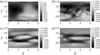
a,b) with some oscillations probably linked to the sinuous instability of the streaks, which is a key process of the self-sustained mechanism of the LB state (see Waleffe Reference Waleffe1997). For large target times, the vortices are localized and smoother, meaning that the sinuous instability has not yet been triggered. The progressive modification of the minimal perturbation with the target time towards a localized structure recalling the minimal seed can be better observed in figure 8, providing the velocity perturbation in the plane
 $x=4.5$
for the minimal perturbations obtained for
 $T=5$
,
 $T=20$
,
 $T=60$
, and
 $T=100$
. The bent streaks characterizing the minimal perturbations at very small target times (see figure 8
a) become more scattered as the target time increases (see figure 8
b for
 $T=20$
). For a further increase of
 $T$
, the regions of large streamwise perturbation become much narrower in the spanwise direction, showing an alternating pattern in the spanwise and wall-normal directions. Finally, for
 $T=100$
, the streamwise component of the perturbation strongly localizes in the spanwise direction (figure 8
d), being characterized by two alternating patches of streamwise disturbance flanked by two asymmetrical vortices, resembling the shape of the minimal seed for plane Couette flow (Monokrousos et al.
Reference Monokrousos, Bottaro, Brandt, Di Vita and Henningson2011; Rabin et al.
Reference Rabin, Caulfield and Kerswell2012; Cherubini & De Palma Reference Cherubini and De Palma2013). It is also worth observing that, for small values of
 $T$
, the perturbation is characterized by very large values of the streamwise velocity component, which progressively decrease with the target time, whereas the crossflow velocity components are initially small, then increase with
 $T$
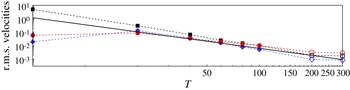
, and finally decrease again. This is clearly shown in figure 9, where the root mean square (r.m.s.) values of the streamwise, wall-normal, and spanwise components of the velocity are provided for all of the target times considered, the black symbols representing the minimal perturbations and the white ones the NLOPs. For
 $20\leqslant T\leqslant 200$
, it appears that the r.m.s. values of the velocity perturbation also follow a power law, which is close to the one found for the energy (although the decrease of
 $w_{rms}$
appears to be slightly less steep), whose slope is indicated by the solid line. As expected, at large target times, such values saturate to some threshold values, having
 $w_{rms}>u_{rms}>v_{rms}$
, whereas at smaller target times
 $u_{rms}$
is the largest component. Also, notice that for
 $T=5$
the r.m.s. values of the velocity have a very different relative magnitude, being characterized by a very large value of
 $u_{rms}$
and a much lower value of
 $v_{rms},w_{rms}$
. In fact, being very close to the edge state, the perturbation does not have enough time to create streamwise perturbation by the lift-up mechanism (Landahl Reference Landahl1980), so it should already be characterized by large values of
 $u_{rms}$
to be able to quickly approach the edge.
Minimal perturbations obtained for (a)
 $T=5$
, (b)
 $T=20$
, (c)
 $T=60$
, and (d)
 $T=100$
in the plane
 $x=4.5$
. The shaded contours represent the positive and negative streamwise component of the velocity perturbation, whereas the vectors represent the wall-normal and spanwise components of the velocity perturbation. Half of the domain is shown in the spanwise direction.

Root mean square values of the streamwise, wall-normal, and spanwise components of velocity (squares,
 $u_{rms}$
; diamonds,
 $v_{rms}$
; circles,
 $w_{rms}$
) versus target time, for the minimal perturbations computed for
 $T\leqslant 100$
and for two NLOPs. The solid line is the
 $T^{-1.75}$
line passing through 1 at
 $T=5$
.

3.2. The minimal-energy route towards the edge state
Direct numerical simulations (DNS) have been performed to analyse the evolution of the minimal perturbations towards the edge state for small to moderate target times,
 $T\leqslant 100$
. The early phases of the evolution of the minimal perturbation computed for
 $T=80$
(called
 $\boldsymbol{u}_{T=80}^{min}$
hereafter) are shown in figure 10, which provides the streamwise vorticity on the
 $z=2{\rm\pi}$
plane at three different time instants,
 $t=0,5,10$
. The vortices are tilted in the streamwise direction very quickly, already leading to a positive inclination at
 $t=5$
, and inducing an energy growth by the Orr mechanism. This energy-growth mechanism, being essentially two-dimensional, acts on the spanwise vorticity, increasing the streamwise and wall-normal components of the velocity perturbation, until a positive inclination is reached (Orr Reference Orr1907).
Snapshots of the perturbation at (a)
 $t=0$
, (b)
 $t=5$
, (c)
 $t=10$
, in the plane
 $z=2{\rm\pi}$
for a DNS initialized by the minimal perturbation for
 $T=80$
. The contours represent the positive and negative streamwise vorticity perturbation.

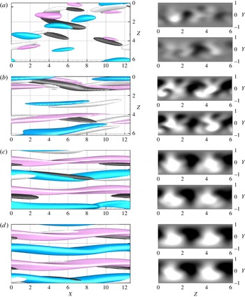
Figure 11 shows four snapshots of the isosurfaces of the streamwise velocity (pink and blue) and vorticity (black and white) extracted from a DNS initialized by
 $\boldsymbol{u}_{T=100}^{min}$
. Figure 11(a) shows the unpacking of the initially localized perturbation into several similar structures composed by opposite inclined vortices and patches of streamwise perturbation. It is noteworthy that this snapshot, extracted at
 $t=10$
for
 $\boldsymbol{u}_{T=100}^{min}$
, is similar to the initial minimal perturbation obtained for
 $T=80$
(see figure 6
d), indicating that the minimal perturbations computed for different target times may share some important features in their route towards the edge state. Figure 11(b) shows that at
 $t=30$
the vortices are stretched in the streamwise direction and begin to produce, by means of the lift-up mechanism, elongated patches of streamwise perturbation, which are already strongly inclined and modulated in the streamwise and spanwise direction. At
 $t=50$
(figure 11
c), these patches of streamwise perturbations begin to merge to create bent streaks, having weak streamwise vortices on their flanks. Finally, the perturbation appears to slowly relax onto the edge, as shown in figure 11(d) for
 $t=70$
.
Snapshots of the perturbation at (a)
 $t=10$
, (b)
 $30$
, (c)
 $50$
, and (d)
 $70$
, for a DNS initialized by the minimal perturbation
 $\boldsymbol{u}_{T=100}^{min}$
. The white and black surfaces represent the positive and negative spanwise velocity components: (a–d)
 $w=\pm (0.6,0.4,0.2,0.17)$
. Blue and pink represent the negative and positive streamwise velocity components: (a)
 $u=\pm 0.17$
, (b–d)
 $u=\pm 0.32$
. The right frames show the contours of the streamwise velocity component at
 $x=1$
(lower) and
 $x=4$
(upper), extracted from the DNS for each of the times considered.

In order to check the convergence of the minimal perturbations on the lower-branch solution, we have computed the correlation with the LB state during the time evolution of these perturbations. The correlation defined by Kerswell & Tutty (Reference Kerswell and Tutty2007) has been used to define the passage of the perturbation
 $\boldsymbol{u}_{DNS}$
in the close vicinity of the edge state
 $\boldsymbol{u}_{ES}$
, such as
 $$\begin{eqnarray}C=\max _{x,z}\left[\frac{\langle \boldsymbol{u}_{DNS},\boldsymbol{u}_{ES}\rangle }{\sqrt{\langle \boldsymbol{u }_{DNS},\boldsymbol{ u }_{DNS}\rangle \langle \boldsymbol{u }_{ES},\boldsymbol{ u }_{ES}\rangle }}\right].\end{eqnarray}$$
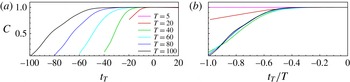
Figure 12(a) shows the correlation value
 $C$
versus the time to the target, defined as
 $t_{T}=t-T$
. One can clearly observe that the correlation value remains close to one for a long time while approaching the edge state, and that when increasing the target time the perturbation stays longer in the vicinity of the edge. Moreover, the minimal perturbations computed for
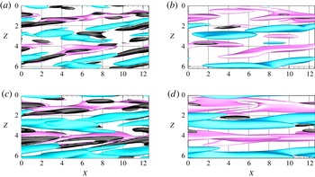
 $T\geqslant 40$
show a very similar shape of the correlation curves: they all approach the edge state in a relatively short time, since they reach
 $C>0.9$
in approximately
 $t<T/2$
, and stay close to it for a time interval that is longer for greater
 $T$
. To further verify the similarity of the trajectories, we have scaled the time with respect to the target time. Figure 12(b) shows the correlation versus the scaled time to the target,
 $t_{T}/T$
. One can observe that the correlation curves associated with the minimal perturbations
 $\boldsymbol{u}_{T=40,60,80,100}^{min}$
are almost superposed, whereas those for
 $\boldsymbol{u}_{T=5,20}^{min}$
have a different shape (in particular, for
 $T=5$
the perturbations stay very close to the edge during the whole time evolution).
Correlation between the edge state and the minimal perturbations computed for different
 $T$
versus the time to the target,
 $t_{T}=t-T$
(a) and the normalized time
 $t_{T}/T$
(b).

To verify that the main energy growth mechanisms followed by
 $\boldsymbol{u}_{T=100}^{min}$
are shared by the other minimal perturbations obtained for
 $T\geqslant 40$
, we have compared the flow structures extracted at different instants of time during the evolution of the minimal perturbations
 $\boldsymbol{u}_{T=40,80}^{min}$
towards the edge state. To take into account the fact that the larger the target time, the slower the evolution towards the edge, we have compared the snapshots taken at the same normalized time. Figure 13 shows the snapshots of both perturbations at
 $t/T=1/4,3/8$
, namely
 $t=10,15$
for
 $\boldsymbol{u}_{T=40}^{min}$
and
 $t=20,30$
for
 $\boldsymbol{u}_{T=80}^{min}$
. One can observe that the streamwise perturbations (pink and blue) are rather similar (although not identical) at different target times, whereas the spanwise and wall-normal velocity components (black) are very different. In particular, these components have different amplitudes for different
 $\boldsymbol{u}_{T}^{min}$
, and these amplitudes are found to be larger for smaller target times.
Snapshots of the perturbation for two direct numerical simulations initialized by the minimal perturbations at
 $T=40$
(a,c) and
 $T=80$
(b,d), extracted at (a,b)
 $t/T=1/4$
, (c,d)
 $t/T=3/8$
. The pink and blue surfaces represent the positive and negative streamwise component of the velocity perturbation:
 $u=\pm 0.25$
. Black represents the wall-normal velocity component: (a,b)
 $v=-0.06$
, (c,d)
 $v=-0.035$
.

Root mean square values of the streamwise, wall-normal, and spanwise components of velocity (a–c
 $u_{rms},v_{rms},w_{rms}$
) versus the time to the target
 $t_{T}$
, for the minimal perturbations computed for
 $T=5,20,40,60,80,100$
.

These differences in the growth of the velocity components can be further analysed by looking at the time evolution of the r.m.s. values of the streamwise, wall-normal and spanwise components of the velocity which represent the streaks, the streamwise vortices and the sinuous mode inducing the streaks bending, respectively. In fact, it is known that the LB state is self-sustained by a process based on the mutual generation of streaks and vortices (Wang et al.
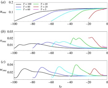
Reference Wang, Gibson and Waleffe2007). Thus, the evolution of the energy associated with streaky and vortical structures may provide some clues as to the efficient development of such a self-sustained process (in terms of both time and energy). Figure 14(a) shows the growth of the r.m.s. value of the streamwise velocity components versus the time to the target
 $t_{T}$
. The slope of the
 $u_{rms}$
growth curve is large at small times, and decreases in time towards a final saturation. One can observe that the saturation phase is much longer for large target times (reaching 40 time units for the minimal perturbation obtained for
 $T=100$
), whereas it is much shorter for smaller target times. On the other hand, the
 $v_{rms}$
and
 $w_{rms}$
behave differently (see figure 14
b,c, respectively), since they peak at small times and then decrease towards the low value characterizing the LB state. In particular, for
 $T\geqslant 40$
the
 $v_{rms}$
curve has a double peak, whereas
 $w_{rms}$
has only one peak, which is placed in correspondence with the
 $v_{rms}$
local minimum. Moreover, the initial values of
 $v_{rms}$
and
 $w_{rms}$
are similar, but the latter grows more than the former. All of the r.m.s. curves for
 $T\geqslant 40$
are similar in shape, even though the growth phase is shifted in time, stretched or compressed depending on the target time, and different in amplitude. In particular, the first peak of
 $v_{rms}$
occurs at
 $t\approx 5$
for all of the curves considered, which is very close to the time at which the initial vortices are straightened by the base flow up to an angle close to
 ${\rm\pi}/2$
with respect to the streamwise direction (see figure 10
b at
 $t=5$
). In fact, when such vortices are straightened up starting from an initial inclination opposed to the mean flow, the growth of the spanwise vorticity is induced by the Orr mechanism, leading to the increase of both
 $u_{rms}$
and
 $v_{rms}$
(Orr Reference Orr1907). At larger times, the
 $u_{rms}$
continues to grow due to the modified lift-up mechanism, linked to the transport of the base-flow shear by the localized modulated vortices (see Cherubini et al.
Reference Cherubini, Robinet, Bottaro and De Palma2011), whereas
 $v_{rms}$
starts to decrease before increasing again due to nonlinear interactions (see the discussion of the Waleffe low-dimensional model below). All of the r.m.s. curves for
 $T\geqslant 40$
show similar behaviour, but it is noteworthy that for smaller target times the maximum amplitude for the
 $v_{rms},w_{rms}$
curves is found to increase. On the other hand, the r.m.s. curves for
 $T<40$
show a rather different shape, probably because the perturbation does not have time to exploit all of the growth mechanisms. In fact,
 $v_{rms}$
has an initial value larger than
 $w_{rms}$
and shows only one peak, which does not correspond to a local minimum of
 $v_{rms}$
.
(a) Perturbation energy and (b–d) r.m.s. values of the streamwise, wall-normal, and spanwise components of velocity versus the normalized time
 $t/T$
for the minimal perturbations computed for
 $T=5,20,40,60,80,100$
.

Figure 14 indicates that the minimal perturbations computed for different target times do not follow the same trajectory; however, the r.m.s. curves associated with the minimal perturbations for
 $T\geqslant 40$
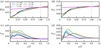
appear to share the main features of the perturbation dynamics on different time scales. In order to better visualize these similarities, we have plotted the r.m.s. values of the velocity perturbations, as well as the perturbation energy, versus the normalized time
 $t/T$
, as shown in figure 15. Figure 15(a,b) shows that the energy and
 $u_{rms}$
curves are very close to each other for
 $T\geqslant 40$
, whereas they have a much lower slope for
 $T=20$
and
 $T=5$
(especially for the latter case in which the perturbation appears to be already in the saturation phase). On the other hand, figure 15(c,d) shows that, for
 $T\geqslant 40$
, the
 $v_{rms}$
and
 $w_{rms}$
curves are similar in shape, peaking at approximately the same time, but different in amplitude. In particular, the smaller the target time, the larger the
 $v_{rms},w_{rms}$
maximum amplitude. This can be explained by considering the self-sustained process leading to the edge state, using the Waleffe (Reference Waleffe1997) low-dimensional model,
 $$\begin{eqnarray}\displaystyle \left.\begin{array}{@{}l@{}}\text{d}\tilde{u} /\text{d}t=-(k_{u}^{2}/R)\tilde{u} -{\it\sigma}_{w}\tilde{w}^{2}+{\it\sigma}_{u}m\tilde{v},\\ \text{d}\tilde{v}/\text{d}t=-(k_{v}^{2}/R)\tilde{v}+{\it\sigma}_{v}\tilde{w}^{2},\\ \text{d}\tilde{w}/\text{d}t=-(k_{w}^{2}/R)\tilde{w}+({\it\sigma}_{w}\tilde{u} -{\it\sigma}_{m}m-{\it\sigma}_{v}\tilde{v})\tilde{w},\\ \text{d}m/\text{d}t=-(k_{m}^{2}/R)m-{\it\sigma}_{u}\tilde{u} \tilde{v}+{\it\sigma}_{m}\tilde{w}^{2}+k_{m}^{2}/R,\end{array}\right\} & & \displaystyle\end{eqnarray}$$
where
 $\tilde{u} ,\tilde{v},\tilde{w}$
model the amplitudes of the streamwise streaks, the streamwise vortices, and the sinuous perturbations of the streaks, respectively and
 $m$
is the mean shear induced by these perturbations at the Reynolds number
 $R$
. This model describes how the streaks are fed by the vortices, which are sustained in turn by the secondary sinuous modes. In order to lead the perturbation very rapidly on the edge state,
 $\tilde{u} ,\tilde{v},\tilde{w}$
must quickly grow in time. To let
 $\tilde{u}$
grow, since the shear grows on a slow time scale,
 $\tilde{v}$
must be large to compensate the dissipative term as well as the negative term
 $-{\it\sigma}_{w}\tilde{w}^{2}$
. At the same time, to keep
 $\tilde{v}$
growing and generate streaks, a large growth of
 $\tilde{w}^{2}$
is needed. By analogy, this explains the peak values of
 $v_{rms},w_{rms}$
, which must be larger to induce a quicker streak growth and trigger the cycle sustaining the LB state. On the other hand, when a larger target time is available to approach the edge state, the vortices can grow more slowly and up to lower values since they have more time to feed and bend the streaks.
Snapshots of the evolution of the minimal perturbation obtained for
 $T=20$
, at times (a)
 $t=5$
and (b)
 $t=15$
(from top to bottom). The isosurfaces on the left represent the positive and negative streamwise velocity (pink and blue for a,b
 $u=\pm (0.17,0.3)$
) and vorticity components (black and white for a,b
 ${\it\omega}_{x}=\pm (0.5,0.28)$
). The shaded contours on the right represent the streamwise velocity perturbation on the planes
 $x=4$
(upper) and
 $x=9$
(lower) at each of the times considered.

Moreover, the curves of the r.m.s. velocity components in figure 15 indicate that the minimal perturbations approaching the edge state in a very short time (
 $T\leqslant 20$
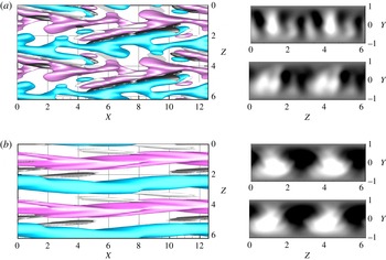
) follow a different route. This is confirmed by looking, in figure 16, at the flow structures induced during the evolution of the minimal perturbation obtained for
 $T=20$
. At
 $t=5$
the alternated patches of streamwise perturbation forming the large part of the minimal perturbation have already merged, creating a rather complex pattern of fingered alternated streaks (see the top frames). Then these fingered streaks begin to be stretched into a strongly bent structure, which at
 $t=15$
relaxes towards the weakly bent streaky structure characterizing the edge state (see the bottom frames for
 $t=15$
). From the results described here it appears that minimal perturbations for
 $T\leqslant 20$
have to maintain at least one of the edge state symmetries to be able to approach it in a very short time. Therefore, they cannot be localized in space and they are characterized by larger values of the velocity components, as discussed in the previous section. On the other hand, minimal perturbations for
 $T\geqslant 40$
can be localized in space and characterized by much lower values of the velocity components, relying on effective energy growth mechanisms to achieve the edge state. The fact that the overall dynamics of these minimal perturbations is very similar but the trajectories to the edge state are different might be linked to the fact that the edge of chaos is folded and probably wrapped around the chaotic saddle. In fact, in the folds of the edge of chaos there may exist many local energy minima which are the origins of (different but) similar trajectories towards the edge, approaching it in a larger or shorter time depending on the initial energy (see figure 2).
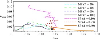
Projected trajectories on the
 $u_{rms}$
–
 $w_{rms}$
plane corresponding to the minimal perturbations (MP) computed for
 $20\leqslant T\leqslant 100$
, and to the linear optimal streaky perturbations (SP) of amplitude
 $A$
, perturbed using a sinuous mode and rescaled by bisection until the edge state is approached.

These trajectories towards the edge state can be traced by projecting the state space onto the
 $u_{rms}$
–
 $w_{rms}$
plane (see Cossu et al.
Reference Cossu, Brandt, Bagheri and Henningson2011), as provided in figure 17. The thin lines in the figure show that all of the minimal-perturbation trajectories start very close to the LS, represented by the origin of the axis (see the rectangular box in the figure) and approach the edge state (represented by the white dot) by rapidly increasing both
 $w_{rms}$
and
 $u_{rms}$
, and finally decreasing
 $w_{rms}$
towards the edge. In particular, the starting points of these trajectories may be viewed as (a projection of) the locus of the local energy-minima of the basin boundary separating the LS from the chaotic saddle. As observed before, the trajectories are very similar and close to each other, but not superposed, indicating once again that the laminar–turbulent boundary has a very complex structure. Moreover, such trajectories are very different from the ones leading other optimal perturbations towards the edge. For example, the thick lines in figure 17 represent the trajectories followed by three saturated linear optimal perturbations, characterized by streamwise streaks of different amplitude
 $A$
, on which a sinuous mode has been superposed and rescaled by bisection until it approaches the edge state (see Cossu et al. (Reference Cossu, Brandt, Bagheri and Henningson2011) for a more detailed description of this procedure). Figure 17 shows that these streaky perturbations (SP) approach the edge by following a very different route, starting in the top or in the right part of the
 $u_{rms}$
–
 $w_{rms}$
plane, where the amplitude of the perturbation is even larger than the one on the edge state, and then decay in an oscillating fashion towards the edge state. Although the starting points of these trajectories are indeed on the laminar–turbulent boundary, these perturbations are very far from the local energy minima on the bottom left part (the rectangular box in figure 17) of the
 $w_{rms}$
–
 $u_{rms}$
plane, indicating the inefficiency (in terms of initial amplitude) of these linear optimal perturbations at inducing transition. On the other hand, the minimal perturbations computed here need a very small initial energy to approach the edge state in a finite time horizon, and could thus be very useful in developing effective control systems aiming to drive perturbations towards the lower branch state.
4. Concluding remarks
Transition to turbulence in shear flows is often subcritical, thus the dynamics of the flow strongly depends on the shape and amplitude of the perturbation of the laminar state. The sequence of flow states composing the transition process defines a trajectory in the state space. In such a space, initial perturbations which directly relaminarize are separated from those that go through a chaotic trajectory by a hypersurface having a very small number of unstable dimensions, known as the edge of chaos. Previous studies have established that the edge of chaos for plane Couette flow is characterized by a fractal (Lebovitz Reference Lebovitz2009; Vollmer et al.
Reference Vollmer, Schneider and Eckhardt2009; Lai & Tél Reference Lai and Tél2011), folded structure, probably wrapped around the chaotic saddle (Lebovitz & Mariotti Reference Lebovitz and Mariotti2013; Chantry & Schneider Reference Chantry and Schneider2014). Thus, the problem of determining a threshold energy to trigger subcritical transition consists in finding the states on this complex hypersurface with minimal distance (in the energy norm) from the laminar state. For this reason, in this work we have investigated the minimal-energy regions of the edge of chaos, by developing a minimization method aiming to determine the minimal-energy perturbations capable of approaching the edge state (within a prescribed tolerance) in a finite time. Previous studies have determined the ‘minimal seed’ for transition, namely the perturbation of minimal energy asymptotically approaching the edge state (Rabin et al.
Reference Rabin, Caulfield and Kerswell2012), by using an optimization of a functional linked to the turbulence, coupled with a bisection of the initial energy. However, this technique cannot be generalized to obtain perturbations approaching the edge state at small target times, since other optimal branches appearing at small target times may mask the minimal seed (Rabin et al.
Reference Rabin, Caulfield and Kerswell2012). Thus, we have developed a different approach, namely a minimization based on the Lagrange multiplier technique, including in the minimization functional both the distance from the edge at a target time
 $T$
and the initial energy. For the sake of simplicity, we have considered plane Couette flow in a small domain, at Reynolds number equal to 400, for which a steady edge state exists (Schneider et al.
Reference Schneider, Gibson, Lagha, De Lillo and Eckhardt2008).
For sufficiently small target times (
 $40\leqslant T\leqslant 200$
), the value of the minimal energy has been found to vary with
 $T$
following a power law, whose best fit is given by
 $E_{min}\propto T^{-1.75}$
. For large values of
 $T$
, the minimal energy achieves a constant value which corresponds to the energy of the minimal seed. This power law allows one to determine the threshold values of the initial energy required to approach the edge state in a given time interval. We have thus established that, for the case of plane Couette flow, even if the structure of the edge of chaos is very complex, the threshold energy for transition not to occur at a given time can be expressed by a very simple law.
The local energy minima on the edge of chaos have been further analysed by looking at the structure of the minimal perturbations approaching the edge state at time
 $T$
. In particular, we have found that, for small values of the target time (
 $T<40$
), the minimal perturbations keep the spanwise translation symmetry of the edge state, whereas for
 $T\geqslant 40$
, all of the symmetries of the edge state are broken and the perturbation appears to be localized in space. These localized minimal perturbations are characterized by a repeated basic structure composed of scattered patches of streamwise velocity with inclined streamwise vortices on their flanks which strongly recall the NLOPs found by Cherubini & De Palma (Reference Cherubini and De Palma2013) for plane Couette flow. For sufficiently large target times, the minimal perturbations become very similar to the minimal seed, which is strongly localized in space and optimally growing in time, although they largely differ from it at short times. Furthermore, we have found that, to keep the initial energy at a minimum, the perturbations are initially characterized by low values of the three components of velocity, but they induce peaks of the wall-normal and spanwise velocities, indicating the presence of vortices and streak bending, respectively. Although minimal perturbations obtained for different target times do not follow exactly the same trajectory towards the edge, their routes are characterized by very similar mechanisms as long as
 $T\geqslant 40$
. The time evolution of the r.m.s. values of the streamwise, wall-normal and spanwise velocity components appears to follow the same trend for different target times (for
 $T\geqslant 40$
). In particular, the streamwise perturbation velocity curves are found to be almost identical when scaled in time with respect to
 $T$
, whereas the wall-normal and spanwise velocity components present different peak values, whilst being very similar in shape. Moreover, the larger the target time, the lower the wall-normal and spanwise velocity peak values, since the streaks have more time to be generated. This indicates that, for a large enough target time, a very robust mechanism of energy growth exists, able to rapidly bring the perturbations towards the edge state with minimal energy. On the other hand, for
 $T\leqslant 20$
the dynamics of the minimal perturbation appears to be different, since the perturbations do not have enough time to exploit the energy growth mechanisms allowing small localized disturbances to unpack and approach the edge.
Finally, we have found that minimal perturbations originate in a small low-energy zone of the state space, and follow similar trajectories approaching the edge state. Such trajectories are very different from those of linear optimal disturbances, which need very high initial amplitudes and follow inefficient routes towards the edge. The fact that the trajectories of the minimal perturbations, as well as the main mechanisms leading them to transition, are very similar but not identical for different target times, further indicates that the edge of chaos has a complex structure and is thus characterized by many local energy minima, probably located in different folds (or layers) of the laminar–turbulent boundary.
Outlook
Since the edge of chaos is in general characterized by a very small number of unstable dimensions (whereas the dynamics in the turbulent regime is highly unstable), investigating the structure of this hypersurface represents an opportunity to unravel the dynamics of self-sustaining coherent structures recurring in turbulent flows. In particular, finding the minimum energy states on this hypersurface, which are the ‘closest’ ones to the laminar state, may give important indications as to the most efficient path to transition. In this paper we have provided some contributions to this issue. By fixing the time to approach the edge state, we have been able to determine threshold values of both the initial energy and the time for transition. This allowed us to determine the minimum time required by perturbations having a certain ‘distance’ (in the energy norm) from the laminar state to approach the edge state. The fact that the energy of the minimal perturbations scales following a power law,
 $E_{min}\propto T^{-1.75}$
, guarantees that perturbations having energy lower than this threshold cannot reach chaos at a time
 $t<T$
. This result may have important outcomes in the setting of the noise level in experimental or numerical set-ups for staying close to the laminar attractor for long enough, or, vice versa, to reach turbulence in a given short time. Moreover, the structure of the minimal perturbations and their evolution towards the edge state provide a description of the topology of the edge of chaos through its local energy minimum. The fact that minimal perturbations computed for different target times do not follow the same trajectory, confirms that the edge of chaos has a complex structure in its minimal-energy region too, with local energy minima probably located in different folds (or layers) of the laminar–turbulent boundary. However, these trajectories share many features, giving important indications as to the type of perturbations that can rapidly approach the edge state with minimal energy. The knowledge of the shape of the minimal perturbations approaching the edge state might be useful in setting up shear-flow control strategies aiming to target the edge state in order to move from the turbulent side of the edge to the laminar one, as suggested recently by several authors.
At the moment, the results we have found concerning the structure of the edge of chaos are only valuable for the case of plane Couette flow in small domains, whereas in larger domains a more complex picture appears, the edge of chaos being populated by more than one relative attractor. However, the minimization technique presented here can be very easily extended to the case of multiple edge states, once these solutions have been obtained numerically. In fact, the minimization proposed in this work can be performed for each of the computed edge states without any modification of the algorithm (simply by changing the velocity field
 $\boldsymbol{u}_{ES}$
) and the values of the minimal energy for each of these edge states could be compared afterwards. Future work will aim to extend the results presented in this paper to different Reynolds numbers or domain lengths, as well as to cases in which the edge state is time-dependent. In particular, the case of periodic orbits may be easily treated by performing minimizations in different Poincaré sections of the state space, finally selecting the section providing the minimal initial energy. A similar procedure may be used to take into account chaotic edge states, although the analysis must be restrained to a very limited number of phase points.
Acknowledgements
The authors would like to thank A. Bottaro, R. Kerswell, J.-C. Robinet and O. Semeraro for useful discussions about this work.