1 Introduction
The motion of the free liquid surface in a closed basin is encountered in many industrial applications and can have a detrimental effect on the stability of liquid carriers and aerospace vehicles (Ibrahim, Pilipchuk & Ikeda Reference Ibrahim, Pilipchuk and Ikeda2001; Ibrahim Reference Ibrahim2005; Veldman et al. Reference Veldman, Gerrits, Luppes, Helder and Vreeburg2007; Faltinsen & Timokha Reference Faltinsen and Timokha2009). In the case of a harmonic forcing imposed on the container, the wave amplitude increases significantly at resonance. If the amplitude of sloshing motion becomes large enough, geyser formation, wave overturning (Royon-Lebeaud, Hopfinger & Cartellier Reference Royon-Lebeaud, Hopfinger and Cartellier2007) and spilling (Mayer & Krechetnikov Reference Mayer and Krechetnikov2012) can occur, thus potentially affecting safety and operational efficiency. With the purpose of reducing sloshing motion at resonance, tanks have been designed in such a way to change the system’s natural frequencies with respect to the ones of possible excitations, or to increase viscous dissipation. Dissipation devices such as rigid lids and elastic membranes at the free surface or baffles placed in the container, are widely used. Another option consists in designing fuel tanks filled with a porous medium or Hele-Shaw cells, as proposed for tanks of aerospace vehicles (Dwyer & Erickson Reference Dwyer and Erickson1969). This last solution consists in a narrow container where the separation between two plates is small compared to the other two dimensions. In this way viscous friction is enhanced and viscous forces dominate over inertial ones. Interestingly, due to the strong confinement, the transversal velocity is negligible with respect to the in-plane components, and the resulting motion is nearly two-dimensional.
More generally, Hele-Shaw cells have been adopted over the years to study two-phase flows, providing useful insight into viscously driven instability phenomena. A paradigmatic example is the viscous fingering formation, also called Saffman–Taylor instability, that occurs when a less viscous fluid is injected into a Hele-Shaw cell filled with a different immiscible and more viscous fluid. The interface between the fluids develops an instability, leading to the formation of finger-like patterns (Saffman & Taylor Reference Saffman and Taylor1958; Bensimon et al. Reference Bensimon, Kadanoff, Liang, Shraiman and Tang1986).
The mathematical description of the flow in a Hele-Shaw cell is based on the parabolic flow profile approximation in the narrow direction. The in-plane mean velocity
 $\langle \boldsymbol{u}\rangle$
is thus proportional to the pressure gradient, with the proportionality constant scaling inversely with the viscosity,
 $\unicode[STIX]{x1D707}$
, and with the cell gap square,
 $\unicode[STIX]{x1D701}^{2}$
 $$\begin{eqnarray}\langle \boldsymbol{u}\rangle =-\frac{\unicode[STIX]{x1D701}^{2}}{12\unicode[STIX]{x1D707}}\unicode[STIX]{x1D735}p.\end{eqnarray}$$
This is nothing more than the Darcy equation that governs flows in porous media, which are widely studied in geophysics, for instance in the context of oil recovery. Darcy’s law, however, is not valid in cases where inertia, through the advection of momentum, plays a relevant role, such as waves (Kalogirou, Moulopoulou & Bokhove Reference Kalogirou, Moulopoulou and Bokhove2016) and Kelvin–Helmholtz instability in a Hele-Shaw cell, where the instability threshold was found by Gondret & Rabaud (Reference Gondret and Rabaud1997) to be governed by inertial effects. It is not mathematically straightforward to consistently reintroduce convective terms in the depth-averaged Hele-Shaw equations (see Ruyer-Quil Reference Ruyer-Quil2001; Plouraboué & Hinch Reference Plouraboué and Hinch2002).
In this work, we consider the case of inertial effects in a Hele-Shaw cell flow limited to the unsteady term in the Navier–Stokes equations. This scenario corresponds to a pulsatile flow where the fluid’s motion reduces to a two-dimensional oscillating Poiseuille flow (similarly to the Womersley flow in arteries (Womersley Reference Womersley1955)) and it is well suited to investigate sloshing waves in narrow containers, which is the main aim of this work. Our approach is to perform experiments in a narrow cell of fixed gap exposed to a lateral harmonic forcing of angular frequency,
 $\unicode[STIX]{x1D714}$
. The boundary layer to cell’s gap ratio,
 $\unicode[STIX]{x1D6FF}^{\prime }/\unicode[STIX]{x1D701}$
, is varied by filling the cell with liquids of different viscosities,
 $\unicode[STIX]{x1D708}$
, up to the point the thickness of the oscillating boundary layers,
 $\unicode[STIX]{x1D6FF}^{\prime }=\sqrt{2\unicode[STIX]{x1D708}/\unicode[STIX]{x1D714}}$
, becomes comparable to the cell gap,
 $\unicode[STIX]{x1D701}$
, and, as a result, the dissipation is intense in the whole fluid volume, in contrast to the case of large containers. The amplitude and phase of the free-surface shape are monitored. The experimental results are then rationalized through a generalized Darcy’s law for oscillating flows, and the analytical model is then compared to the experimental data.
2 Experimental methods
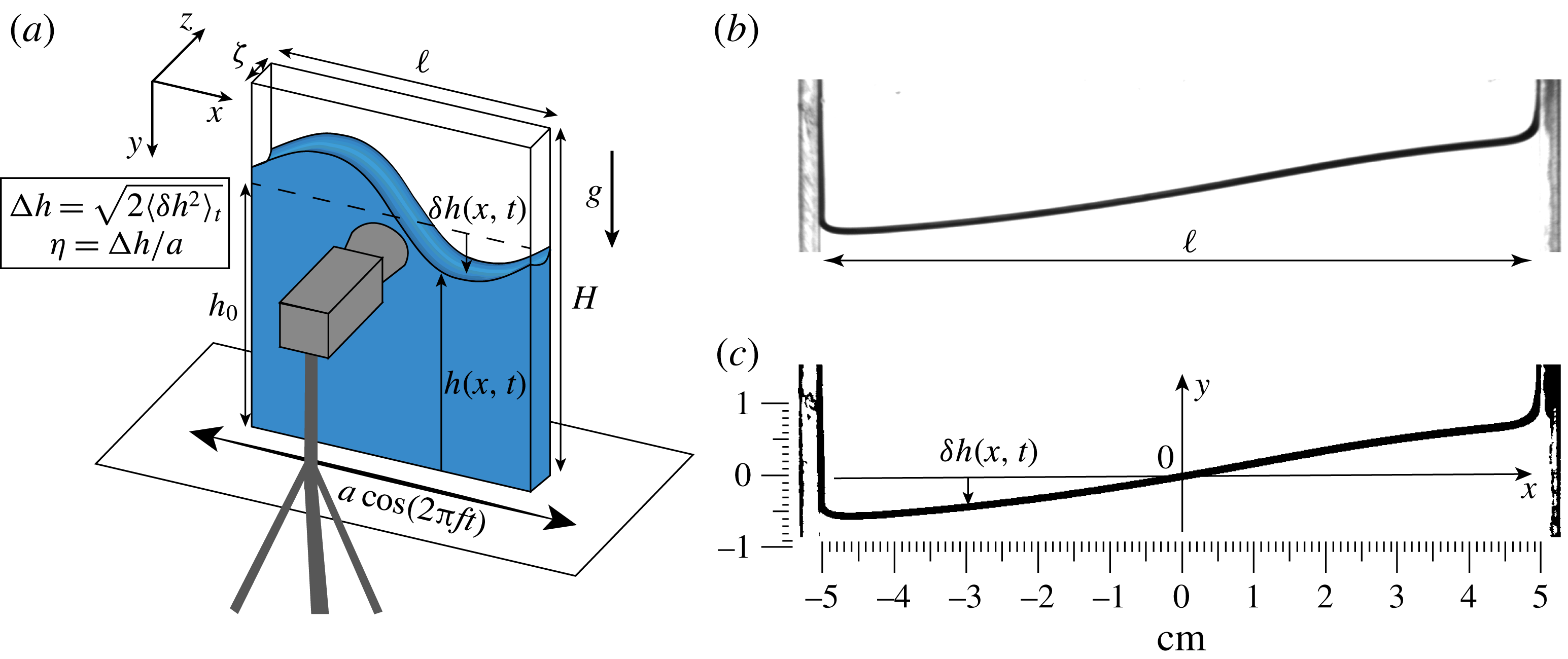
The experimental set-up used to generate the sloshing waves in the narrow container and to measure the free-surface displacement is shown in figure 1(a). A Plexiglas cell of height
 $H=15$
cm, length
 $\ell =10$
cm and width
 $\unicode[STIX]{x1D701}=0.3$
cm is fixed to a single-axis linear motion actuator (Aerotech PRO 165). The container is partially filled from the top with a column of liquid of height
 $h_{0}=10~\text{cm}$
, that is of the same order as the container’s length,
 $h_{0}\approx \ell$
, in order to limit viscous dissipation at the bottom of the container. Indeed, the effect of a finite depth
 $h_{0}/\ell$
enters the eigenfrequency of the fundamental mode, which is the most sensitive to finite-depth effects, through a factor
 $\sqrt{\tanh (\unicode[STIX]{x03C0}h_{0}/\ell )}$
, which equals the infinite-depth limit within less than 1 % for
 $h_{0}=\ell$
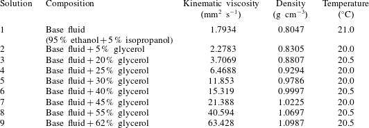
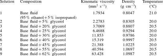
(Ibrahim Reference Ibrahim2005). We use different solutions of 95 % ethanol plus 5 % isopropanol that is mixed with glycerol (0 %, 5 %, 25 %, 40 %, 45 %, 55 % and 62 % in volume of glycerol). The properties of the different solutions are measured with an Anton Paar viscosimeter (SVM 3000) and summarized in table 1.
(a) Sketch of the experimental set-up. (b) Raw image of the air/liquid interface, taken from the experiment without added glycerol and at a forcing frequency of 3.5 Hz. (c) Binarized image obtained after thresholding.

Physical properties of the solutions used at the temperature of the experiments.
Sloshing is generated by imposing a lateral harmonic motion of angular frequency
 $\unicode[STIX]{x1D714}=2\unicode[STIX]{x03C0}f$
, and amplitude
 $a$
. The actuation is set and controlled by the Aerotech Soloist CP software and spanning in sequence the frequency range from
 $f=0.1$
Hz to
 $f=4.5$
Hz with a step of 0.1 Hz. The oscillation amplitude imposed on the cell is set equal to
 $a=6$
mm, which was seen to generate sloshing waves in the linear regime (see § 4 for further details). To ensure that the steady regime is reached, the free-surface dynamics is recorded only after a certain number of cycles, typically 15, through a Blaser camera coupled with a Nikon
 $18{-}108/2.5$
lens. The acquisition frequency is adapted to the excitation frequency: 5 frames per second (f.p.s.) for
 $f\leqslant 0.4$
Hz, 25 f.p.s. for
 $0.5~\text{Hz}<f<0.9$
Hz, and 50 f.p.s. for
 $f>1$
Hz. Lighting is provided by a LED panel (
 $25~\text{cm}\times 15~\text{cm}$
) placed behind the cell. Due to the dependence of viscosity on temperature and high volatility of ethanol, experiments are performed within short time scales, typically less than 30 min, thus avoiding in this way fluid evaporation, and the room temperature is recorded for each experiment. The liquid level is measured before and after the experiment to ensure fluid evaporation is negligible.
In order to extract the location of the air/liquid interface, one needs first to subtract the horizontal motion of the cell, since the camera is not attached to the vibrated tank. To track its vertical central axis
 $y$
, we threshold and binarize each image (figure 1
b,c). The external edges of the cell then appear as black vertical lines (figure 1
c), which are automatically detected in a home-made Matlab program. The
 $y$
axis is set as the middle line between these two edges. The interface appears as a bold black line, because of meniscus effects. We simply describe the interface by a curve of equation
 $y=h(x,t)$
, with
 $h$
being taken as the position of the top of the bold line. We checked that, apart from an offset irrelevant to the dynamics and practically constant along all experiments, defining
 $h$
by the middle line or the bottom of the bold line would not change anything. The relevant quantity describing the interface is actually the deviation of
 $h$
from the interface position at rest
 $h_{0}$
,
 $\unicode[STIX]{x1D6FF}h(x,t)=h(x,t)-h_{0}$
. From this, we deduce the time-averaged amplitude of the interface motion
 $\unicode[STIX]{x0394}h(x)$
and phase difference
 $\unicode[STIX]{x1D711}(x)$
between the interface oscillation and the imposed displacement
 $\tilde{a}(t)$
:
 $$\begin{eqnarray}\unicode[STIX]{x0394}h(x)=\sqrt{2\langle \unicode[STIX]{x1D6FF}h(x,t)^{2}\rangle _{t}},\quad \unicode[STIX]{x1D711}(x)=\arccos \left[\langle \tilde{a}(t)\unicode[STIX]{x1D6FF}h(x,t)\rangle _{t}/\sqrt{\langle \tilde{a}(t)\rangle _{t}^{2}\langle \unicode[STIX]{x1D6FF}h(x,t)\rangle _{t}^{2}}\right].\end{eqnarray}$$
Here, time averaging
 $\langle \cdot \rangle _{t}$
is performed over an entire number of cycles. This ensures that if the horizontal displacement is
 $\tilde{a}(t)=a\cos \unicode[STIX]{x1D714}t$
, then the interface displacement is
 $\unicode[STIX]{x1D6FF}h(x,t)=\unicode[STIX]{x0394}h(x)\cos [\unicode[STIX]{x1D714}t+\unicode[STIX]{x1D711}(x)]$
in the case of a pure harmonic motion in time.
3 Theory
Let us consider the response to forcing of a liquid contained in a rectangular container where the cell gap is much smaller than its width
 $\unicode[STIX]{x1D701}/\ell \ll 1$
. The forcing is applied along the direction
 $x$
(see figure 1
a), and consists of an oscillatory motion of amplitude
 $a$
and angular frequency
 $\unicode[STIX]{x1D714}$
. Hence, the acceleration of the cell in the lab frame is
 $-a\unicode[STIX]{x1D714}^{2}\cos \unicode[STIX]{x1D714}t^{\prime }$
. Primed variables, as time
 $t^{\prime }$
here, design dimensional variables, in contrast to their dimensionless counterparts to be introduced later. In the non-inertial frame of the cell, the fluid obeys the continuity equation and the Navier–Stokes equation with a pseudo-force acting in the
 $x$
-momentum:
 $$\begin{eqnarray}\unicode[STIX]{x1D735}^{\prime }\boldsymbol{\cdot }\boldsymbol{v}^{\prime }=0,\quad \frac{\unicode[STIX]{x2202}\boldsymbol{v}^{\prime }}{\unicode[STIX]{x2202}t^{\prime }}+(\boldsymbol{v}^{\prime }\boldsymbol{\cdot }\unicode[STIX]{x1D735}^{\prime })\boldsymbol{v}^{\prime }=-\frac{1}{\unicode[STIX]{x1D70C}}\unicode[STIX]{x1D735}^{\prime }p^{\prime }+\unicode[STIX]{x1D708}\unicode[STIX]{x0394}^{\prime }\boldsymbol{v}^{\prime }-g\boldsymbol{e}_{y}-a\unicode[STIX]{x1D714}^{2}\cos \unicode[STIX]{x1D714}t^{\prime }\boldsymbol{e}_{x},\end{eqnarray}$$
with
 $\boldsymbol{v}^{\prime }=u^{\prime }\boldsymbol{e}_{x}+v^{\prime }\boldsymbol{e}_{y}+w^{\prime }\boldsymbol{e}_{z}$
the velocity field. In all the following, we neglect the nonlinear advection term on behalf of the small amplitude of the oscillations. The equations of motion are then linear, and we can write
 $\boldsymbol{v}^{\prime }(\boldsymbol{x}^{\prime };t^{\prime })=\text{Re}[\hat{\boldsymbol{v}}^{\prime }(\boldsymbol{x}^{\prime })\text{e}^{\text{i}\unicode[STIX]{x1D714}t^{\prime }}]$
and
 $p^{\prime }(\boldsymbol{x}^{\prime };t^{\prime })=\text{Re}[\hat{p}^{\prime }(\boldsymbol{x}^{\prime })\text{e}^{\text{i}\unicode[STIX]{x1D714}t^{\prime }}]$
with
 $\text{i}$
the imaginary unit and
 $\text{Re}$
taking the real part. We henceforth drop the hat, referring to
 $\hat{\boldsymbol{v}}^{\prime }(\boldsymbol{x}^{\prime })$
and
 $\hat{p}^{\prime }(\boldsymbol{x}^{\prime })$
simply as
 $\boldsymbol{v}^{\prime }=(u^{\prime },v^{\prime },w^{\prime })$
and
 $p^{\prime }$
.
Equations are made dimensionless by using
 $\ell$
along the directions
 $x$
and
 $y$
, and
 $\unicode[STIX]{x1D701}$
along direction
 $z$
. The forcing amplitude and frequency provide a scale
 $a\unicode[STIX]{x1D714}$
for the in-plane velocity components, whereas the continuity equation causes the transverse component to scale as
 $\unicode[STIX]{x1D716}a\unicode[STIX]{x1D714}$
, due to the strong confinement in the
 $z$
-direction:
 $\unicode[STIX]{x1D716}\equiv \unicode[STIX]{x1D701}/\ell \ll 1$
. With these choices, the dimensionless spatial scales, velocity components and pressure are written as:
 $$\begin{eqnarray}x=\frac{x^{\prime }}{\ell },\quad y=\frac{y^{\prime }}{\ell },\quad z=\frac{z^{\prime }}{\unicode[STIX]{x1D701}},\quad u=\frac{u^{\prime }}{a\unicode[STIX]{x1D714}},\quad v=\frac{v^{\prime }}{a\unicode[STIX]{x1D714}},\quad w=\frac{w^{\prime }}{\unicode[STIX]{x1D716}a\unicode[STIX]{x1D714}},\quad p=\frac{p^{\prime }}{\unicode[STIX]{x1D70C}\ell a\unicode[STIX]{x1D714}^{2}}.\end{eqnarray}$$
Furthermore, we separate the static and dynamic pressure contributions by setting
 $$\begin{eqnarray}p=x+\frac{g}{a\unicode[STIX]{x1D714}^{2}}y+q.\end{eqnarray}$$
Projecting (3.1) along
 $x$
,
 $y$
and
 $z$
, we thus get the following dimensionless equations at leading order in
 $\unicode[STIX]{x1D716}$
:
 $$\begin{eqnarray}\frac{\unicode[STIX]{x2202}u}{\unicode[STIX]{x2202}x}+\frac{\unicode[STIX]{x2202}v}{\unicode[STIX]{x2202}y}+\frac{\unicode[STIX]{x2202}w}{\unicode[STIX]{x2202}z}=0,\quad \text{i}u=-\frac{\unicode[STIX]{x2202}q}{\unicode[STIX]{x2202}x}+\frac{1}{2}\unicode[STIX]{x1D6FF}^{2}\frac{\unicode[STIX]{x2202}^{2}u}{\unicode[STIX]{x2202}z^{2}},\quad \text{i}v=-\frac{\unicode[STIX]{x2202}q}{\unicode[STIX]{x2202}y}+\frac{1}{2}\unicode[STIX]{x1D6FF}^{2}\frac{\unicode[STIX]{x2202}^{2}v}{\unicode[STIX]{x2202}z^{2}},\quad 0=\frac{\unicode[STIX]{x2202}q}{\unicode[STIX]{x2202}z},\end{eqnarray}$$
where
 $\unicode[STIX]{x1D6FF}=\unicode[STIX]{x1D6FF}^{\prime }/\unicode[STIX]{x1D701}$
compares the thickness of Stokes boundary layer
 $\unicode[STIX]{x1D6FF}^{\prime }=\sqrt{2\unicode[STIX]{x1D708}/\unicode[STIX]{x1D714}}$
to the cell thickness,
 $\unicode[STIX]{x1D701}$
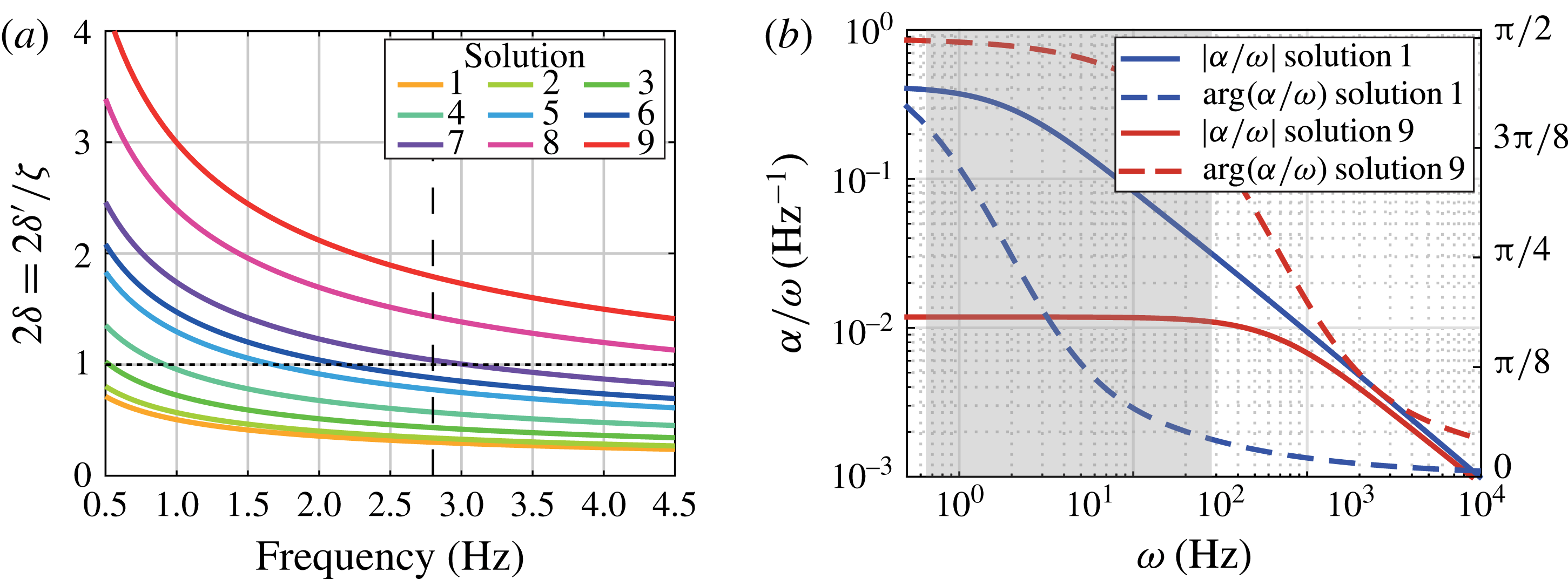
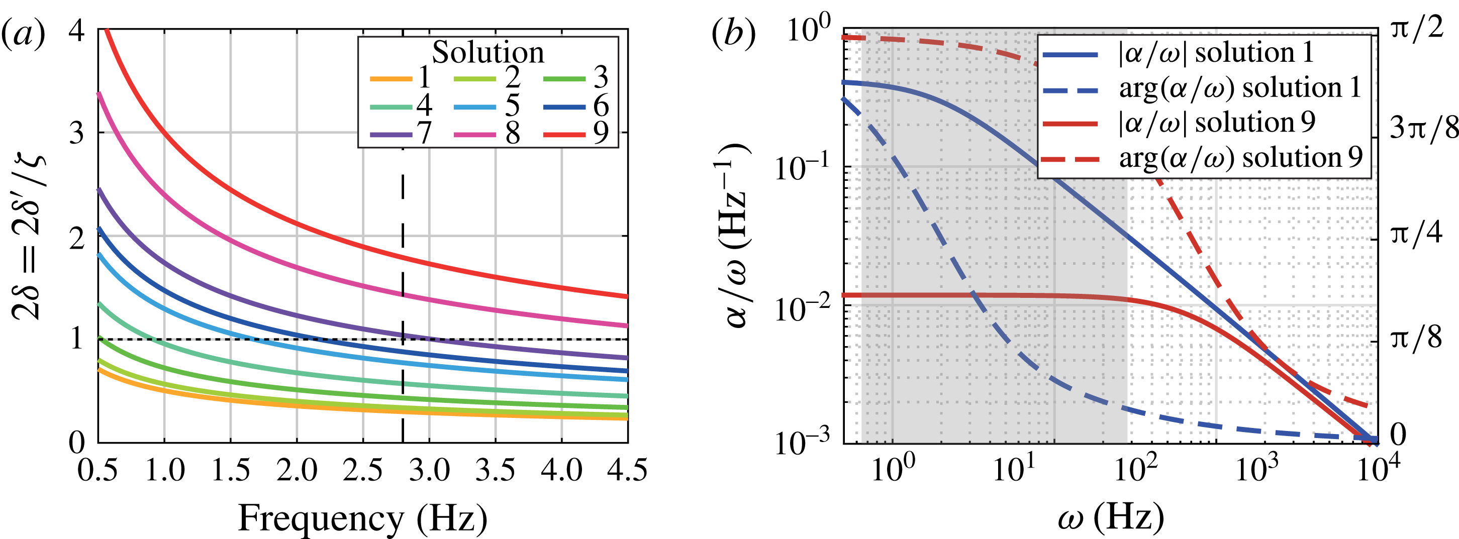
. Figure 2(a) shows
 $2\unicode[STIX]{x1D6FF}$
as a function of the forcing frequency for the different solutions used in the experiments. Note that when
 $2\unicode[STIX]{x1D6FF}=1$
the Stokes layers over the
 $x{-}y$
faces of the cell merge and invade the entire fluid bulk. The dimensionless governing equations (3.4), along with no-slip condition at
 $z=\pm 1/2$
correspond to a two-dimensional pulsatile Poiseuille flow with solution
 $$\begin{eqnarray}u=\text{i}\frac{\unicode[STIX]{x2202}q}{\unicode[STIX]{x2202}x}\left[1-\frac{\cosh (1+\text{i})z/\unicode[STIX]{x1D6FF}}{\cosh (1+\text{i})/2\unicode[STIX]{x1D6FF}}\right],\quad v=\text{i}\frac{\unicode[STIX]{x2202}q}{\unicode[STIX]{x2202}y}\left[1-\frac{\cosh (1+\text{i})z/\unicode[STIX]{x1D6FF}}{\cosh (1+\text{i})/2\unicode[STIX]{x1D6FF}}\right].\end{eqnarray}$$
Therefore, the averaged velocity along
 $z$
satisfies a Darcy-like equation
 $$\begin{eqnarray}\langle \boldsymbol{u}\rangle =\int _{-1/2}^{1/2}\boldsymbol{u}\,\text{d}z=\text{i}\unicode[STIX]{x1D6FC}\unicode[STIX]{x1D735}q,\quad \text{where}~\unicode[STIX]{x1D6FC}=1-\frac{2\unicode[STIX]{x1D6FF}}{1+\text{i}}\tanh \frac{1+\text{i}}{2\unicode[STIX]{x1D6FF}}\end{eqnarray}$$
is the effective permeability taking into account the effect of the depth-averaged pulsatile flow profile. Similarly to Darcy’s law (1.1), equation (3.6) prevents the no-slip condition for the in-plane velocity from being imposed (see appendix A for a boundary layer expansion valid near the lateral walls). Figure 2(b) shows the ratio
 $\unicode[STIX]{x1D6FC}/\unicode[STIX]{x1D714}$
(to which the dimensional solution is proportional) versus the forcing pulsation
 $\unicode[STIX]{x1D714}$
. For sufficiently small frequency, depending on the fluid viscosity,
 $\unicode[STIX]{x1D6FC}/\unicode[STIX]{x1D714}$
becomes constant, thus meaning that the flow profile does not depend on
 $\unicode[STIX]{x1D714}$
and is equal to a quasi-steady Poiseuille flow.
(a) Stokes layer thickness at the walls,
 $2\unicode[STIX]{x1D6FF}^{\prime }$
, over the cell width,
 $\unicode[STIX]{x1D701}$
, as a function of the forcing frequency. Each line corresponds to a different solution used in the experiment, whereas the vertical line depicts the inviscid resonance frequency. (b) Modulus (full line) and phase (dashed line) of
 $\unicode[STIX]{x1D6FC}/\unicode[STIX]{x1D714}$
as a function of
 $\unicode[STIX]{x1D714}$
for the less (blue lines) and most (red lines) viscous solutions used in the experiments. The grey area shows the frequency range covered by the experimental data.
To obtain a governing equation for the
 $z$
-averaged velocity
 $\langle \boldsymbol{u}\rangle$
, we also average the continuity equation. Using the impermeability condition for the spanwise velocity,
 $w=0$
at
 $z=\pm 1/2$
, and (3.5), we find that the pressure field obeys the Laplace equation
 $$\begin{eqnarray}\frac{\unicode[STIX]{x2202}^{2}q}{\unicode[STIX]{x2202}x^{2}}+\frac{\unicode[STIX]{x2202}^{2}q}{\unicode[STIX]{x2202}y^{2}}=0.\end{eqnarray}$$
Looking for solutions by separation of variables with the requirement that they must vanish as
 $y\rightarrow \infty$
(we restrict our analysis to the deep water regime, consistently with experiments), we find that
 $q$
must be of the type
 $$\begin{eqnarray}q=\mathop{\sum }_{n=0}^{\infty }A_{n}\text{e}^{-k_{n}y}\sin k_{n}x,\end{eqnarray}$$
and the no-penetration condition
 $\langle u\rangle =0$
at
 $x=\pm 1/2$
results, through (3.6), in a Neumann condition on
 $q$
and sets the possible wavenumbers to
 $k_{n}=(2n+1)\unicode[STIX]{x03C0}$
, with
 $n\in \mathbb{N}$
.
Let us define the gain
 $\unicode[STIX]{x1D702}$
as the ratio of the displacement of the interface
 $\unicode[STIX]{x0394}h$
to the forcing amplitude
 $a$
,
 $\unicode[STIX]{x1D702}=\unicode[STIX]{x0394}h/a$
, where
 $\unicode[STIX]{x0394}h$
is defined by (2.1). We assume that the slope of the interface remains small, thus, the kinematic boundary condition can be then applied at
 $y=0$
and simplifies to
 $\unicode[STIX]{x2202}\unicode[STIX]{x1D702}/\unicode[STIX]{x2202}t=v$
. Using (3.6), the
 $z$
-averaged kinematic condition can thus be written as
 $\langle \unicode[STIX]{x1D702}\rangle =\unicode[STIX]{x1D6FC}(\unicode[STIX]{x2202}q/\unicode[STIX]{x2202}y)(x,y=0)$
, which, combined with (3.8), yields an equation for the averaged interface position
 $$\begin{eqnarray}\langle \unicode[STIX]{x1D702}\rangle =-\unicode[STIX]{x1D6FC}\mathop{\sum }_{n=0}^{\infty }k_{n}A_{n}\sin k_{n}x.\end{eqnarray}$$
In the case of
 $\ell$
much larger than the capillary length,
 $\ell _{c}=\sqrt{\unicode[STIX]{x1D70E}/\unicode[STIX]{x1D70C}g}$
, with
 $\unicode[STIX]{x1D70E}$
the surface tension (typically
 $\ell _{c}=2~\text{mm}\ll \ell$
in our experiments), surface tension effects are negligible, and the dynamic boundary condition reduces to the continuity of normal stress at the interface. Since the atmospheric pressure is an offset irrelevant to the dynamics, it is simply written as
 $p(x,y=a\unicode[STIX]{x1D702}/\ell )=0$
. From (3.3), we thus get
 $0=x+q(x,y=0)+(g/\ell \unicode[STIX]{x1D714}^{2})\langle \unicode[STIX]{x1D702}(x)\rangle$
, and using (3.8), (3.9) and the Fourier series of
 $x$
in
 $\sin k_{n}x$
, we can solve for the coefficients
 $A_{n}$
. The interface response to the forcing thus reads
 $$\begin{eqnarray}\langle \unicode[STIX]{x1D702}\rangle =\frac{4}{\unicode[STIX]{x03C0}}\unicode[STIX]{x1D6FC}\tilde{\unicode[STIX]{x1D714}}^{2}\mathop{\sum }_{n=0}^{\infty }\frac{(-1)^{n}}{2n+1}\frac{\sin [(2n+1)\unicode[STIX]{x03C0}x]}{\tilde{\unicode[STIX]{x1D714}}^{2}-(2n+1)\unicode[STIX]{x1D6FC}},\end{eqnarray}$$
where
 $\tilde{\unicode[STIX]{x1D714}}=\unicode[STIX]{x1D714}/\unicode[STIX]{x1D714}_{0}$
. Note that when viscosity is small (
 $\unicode[STIX]{x1D6FC}\approx 1$
), we recover the inviscid resonance frequencies,
 $\unicode[STIX]{x1D714}_{n}^{2}=(2n+1)\unicode[STIX]{x03C0}g/\ell$
. In the limit of small frequencies, equation (3.10) reduces to
 $\langle \unicode[STIX]{x1D702}\rangle =-\unicode[STIX]{x03C0}\tilde{\unicode[STIX]{x1D714}}^{2}x$
: the interface assumes a quasi-steady tilted shape prescribed by the acceleration of the cell in the lab frame when
 $\tilde{\unicode[STIX]{x1D714}}^{2}\ll 1$
.
4 Results
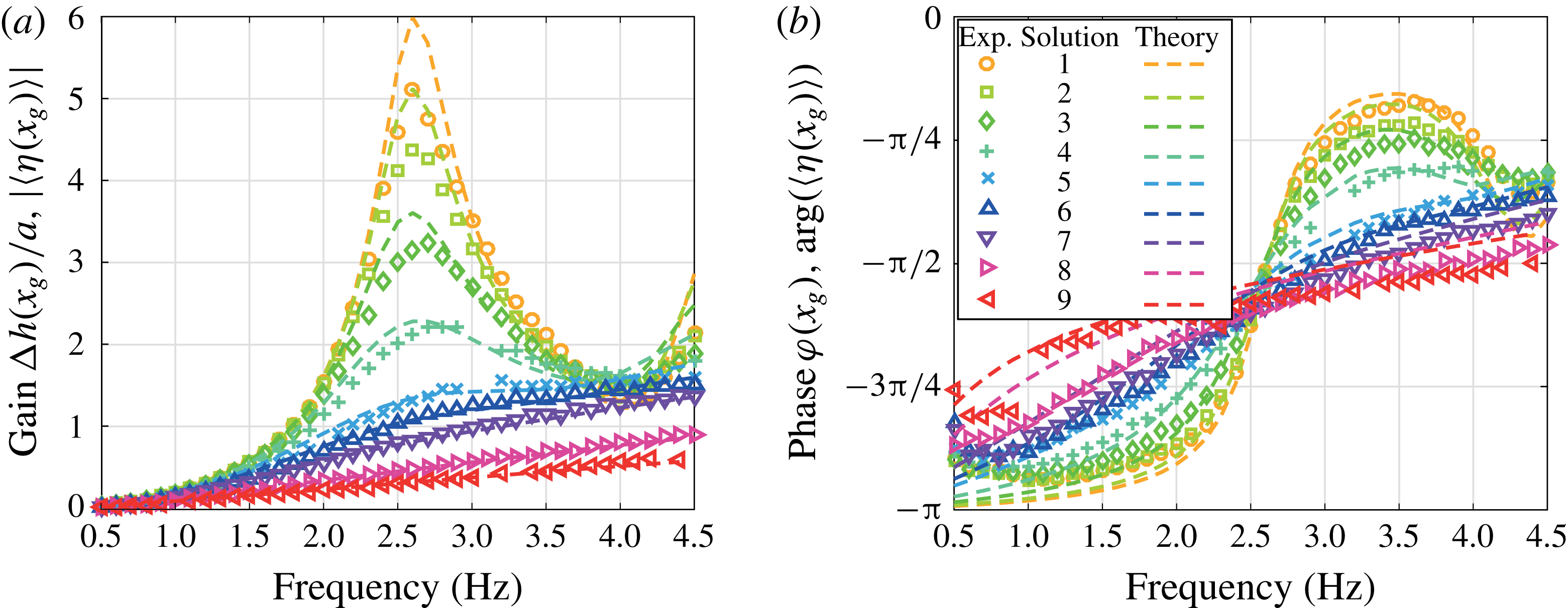
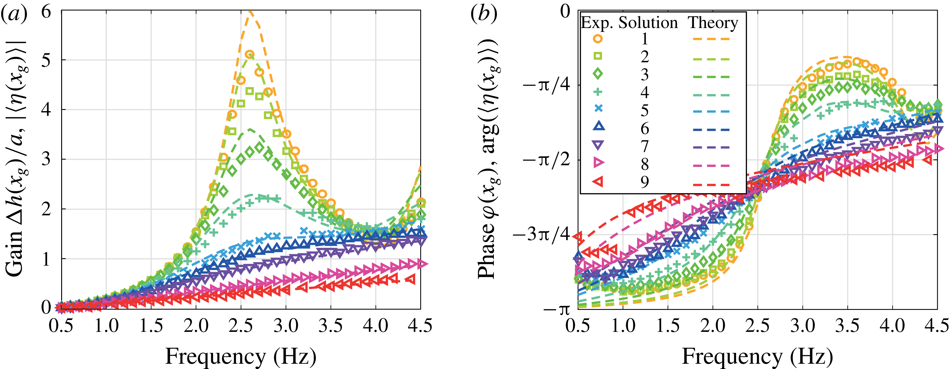
We now present the resonance curves for the different solutions. The time-averaged surface elevation, as defined by (2.1), over the forcing amplitude,
 $\unicode[STIX]{x0394}h(x=x_{g},f)/a$
, is a measure of the energy response of the sloshing wave and is shown in figure 3(a). Here the position
 $x_{g}=45~\text{mm}$
is chosen to be off-centred enough such that the displacement of the interface, hence the signal-to-noise ratio, is maximized, but not too close to the sidewalls as to be influenced by them (see figure 6 and appendix A for a discussion of wall effects). As expected, at any given frequency, the gain is a decreasing function of viscosity. At increasing viscosity, we observe the disappearance of the characteristic resonance peak, which is reminiscent of an underdamped to overdamped transition, for viscosity roughly equal to
 $15~\text{mm}^{2}~\text{s}^{-1}$
(solution 6, see table 1). Note that this transition happens when the fluid bulk at the inviscid resonant frequency is almost completely filled by the oscillating boundary layers. This transition,
 $2\unicode[STIX]{x1D6FF}^{\prime }\approx \unicode[STIX]{x1D701}$
, takes place indeed for a viscosity in between that of solutions 6 and 7, as shown in figure 2(a).
(a) Resonance curves and (b) phase lag for different solution viscosities (see table 1) according to experiments (symbols) and theoretical results (lines). The gain and phase are defined as in (2.1) for the experimental data and as modulus and phase of the average surface elevation (3.10) for the theory.
Experimental resonance curves for the base fluid for forcing amplitudes
 $a=1.5$
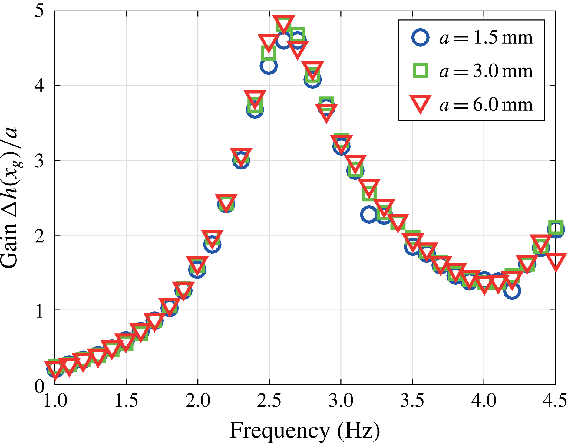
mm (○), 3.0 mm (▫) and 6.0 mm (▿).
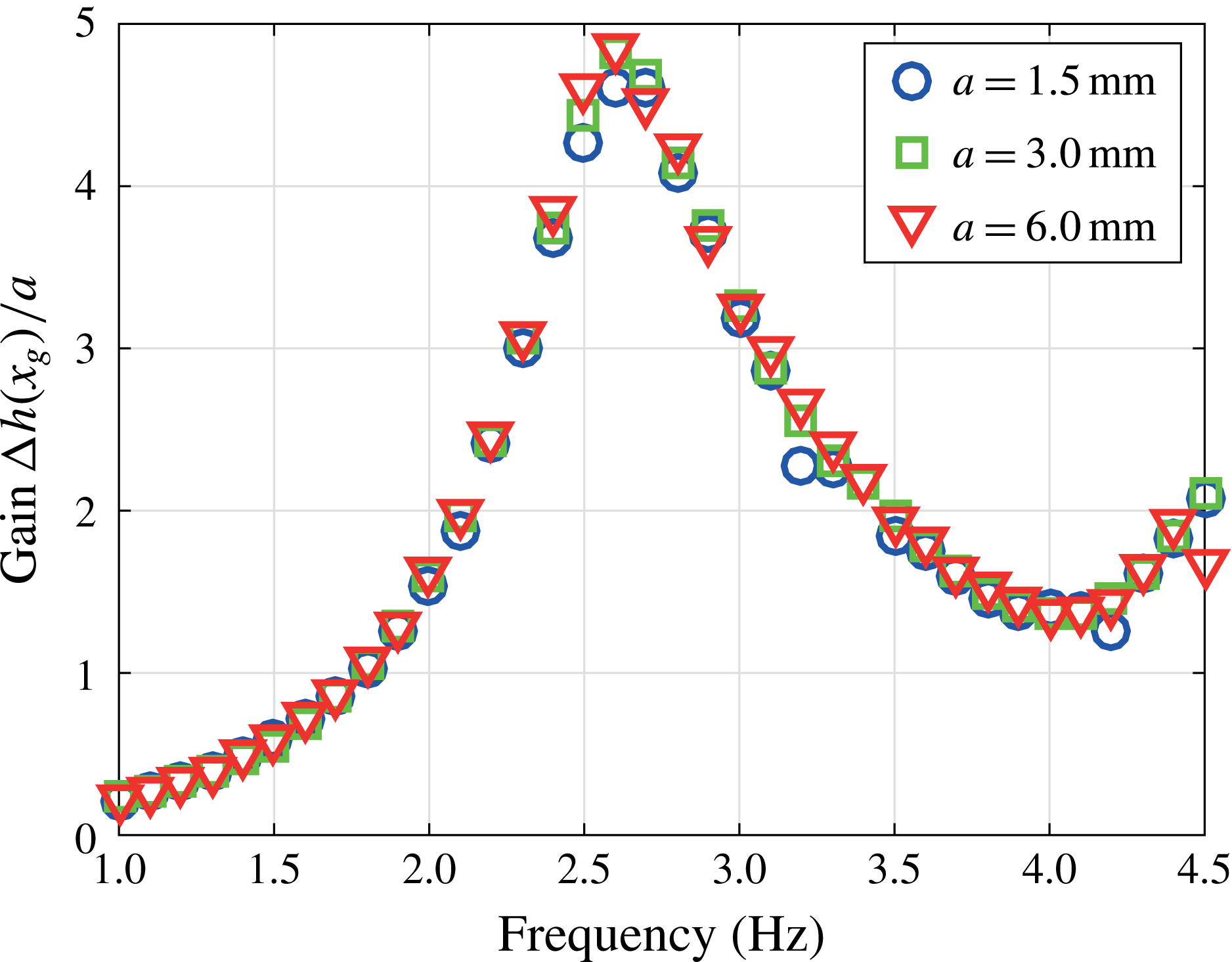
It is important to remark that, as mentioned in § 2, the energy gains reported in figure 3(a) correspond to the linear resonance curves. As a consequence, the maximum wave amplification is here only limited by the viscous dissipation rather than the nonlinear saturation that is expected at larger excitation amplitude. The hypothesis of the linear regime has been verified by varying the forcing amplitude as
 $a=1.5$
, 3.0 and 6.0 mm. The energy gains were found to be unchanged, as shown in figure 4 for base fluid. The other solutions with glycerol, which are more viscous and display oscillations of lesser amplitude, remain in the linear sloshing regime too.
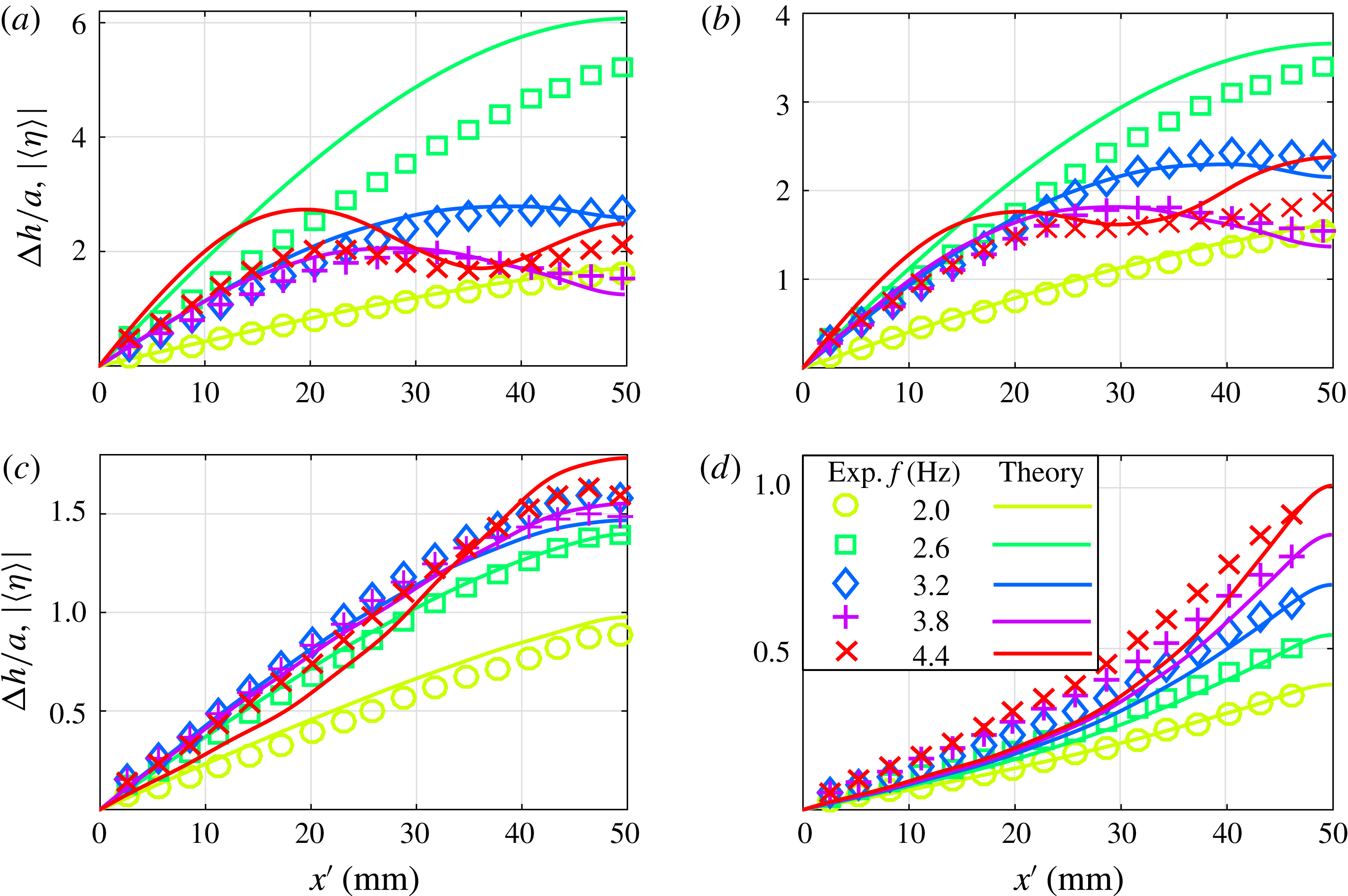
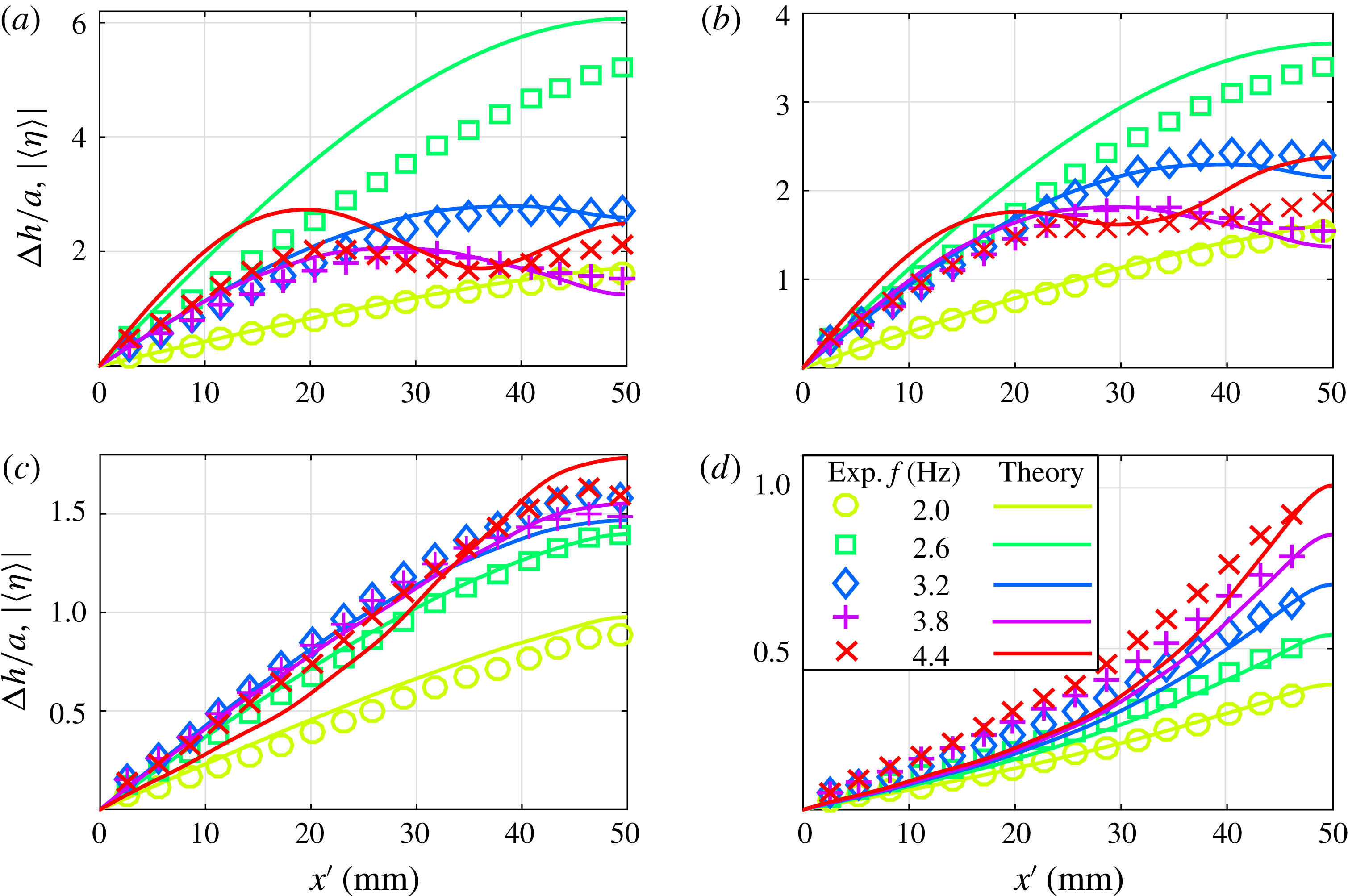
Shape of the oscillating interface at different frequencies according to experiments (symbols) and theory (lines), for different fluid viscosities, namely (a) solution 1, (b) solution 4, (c) solution 6 and (d) solution 8, (see table 1 for the exact fluid properties). Since the data and prediction are symmetric with respect to
 $x=0$
, only the half-cell
 $x>0$
is presented.
This observation therefore allows us to compare the experimental results with our theoretical analysis (§ 3) that is limited to linear sloshing. Assuming that we can identify the experimental measurements of the gain to the
 $z$
-averaged free-surface elevation
 $\langle \unicode[STIX]{x1D702}\rangle$
, the corresponding resonance curves are reported in figure 3(a) (dashed lines). For each solution, the value of the parameter
 $\unicode[STIX]{x1D6FC}$
appearing in (3.10), is evaluated as defined in (3.6) by using the measured viscosity reported in table 1. A good agreement is observed between the experiments and the theory without using any adjustable parameter. In particular, the resonance frequency is well reproduced and the disappearance of the resonance peak precisely captured. The theory, however, overestimates the wave response in the low-viscosity case (namely for solutions 1 and 2) close to the resonance peak, calling for a small additional dissipation to be considered, as discussed in § 5.
In order to get a more complete description about resonant waves in a Hele-Shaw cell, the phase lag between the excitation and the response, as defined in (2.1), is reported in figure 3(b). The phase lag tends to increase from
 $-\unicode[STIX]{x03C0}$
to 0 at increasing frequency, except for the lowest viscosities at frequencies above 3.5 Hz, because of the influence of higher-order modes. For these lowest viscosities which display underdamped resonance, the rate of increase of the phase is maximal at the resonance peak frequency, similarly to a classical forced harmonic oscillator. These measurements are in good agreement with the argument of
 $\langle \unicode[STIX]{x1D702}\rangle$
given in (3.10), further validating our theoretical approach.
In addition to local quantities, we present the shape of the whole oscillating liquid/air interface. Figure 5 shows the experimental and theoretical surface elevation, for a selection of representative frequencies, below (2.0, 2.6 Hz) and above resonance (3.2, 3.8 and 4.4 Hz), and for a set of viscosities in both underdamped and overdamped regime. Below resonance (circles in a–d), the shape of the interface is roughly a tilted line, as prescribed by the acceleration of the cell in the lab, in agreement with the discussion at the end of § 3. At moderate viscosities and close to resonance (squares in a–c)
 $\langle \unicode[STIX]{x1D702}\rangle$
matches a sinusoidal free-edge mode, whereas a tilted line mode is still observed for high viscosity (d). At increasing frequency, the shape becomes more complex, and the gain is no longer a monotonic function of
 $|x|$
for the largest frequencies and the lowest viscosities. In particular, for forcing frequency
 $f=4.4$
Hz higher modes contribute to the dynamics at low and moderate viscosities (see
 $\times$
-symbols in a,b). Although some discrepancies are present, especially at low viscosity (a), our model reproduces the main features of the free-surface shape observed in the experiments.
5 Conclusions and further discussions
In this paper, the behaviour of surface gravity waves in a Hele-Shaw cell subjected to a horizontal oscillation is investigated. The resonance curves are measured experimentally in the low-amplitude regime and the oscillating boundary layer to cell’s gap ratio is varied by filling the cell with liquids of different viscosities. With increasing viscosity and, as a consequence, thickness of the Stokes layers, the viscous forces dominate over the inertial forces and the surface elevation of the sloshing wave decreases. In addition, the fluidic system undergoes to a transition from the underdamped to the overdamped regime when the two Stokes layers over the large faces of the cell fill the fluid bulk (
 $2\unicode[STIX]{x1D6FF}^{\prime }/\unicode[STIX]{x1D701}\approx 1$
). Similarly to a damped harmonic oscillator, the phase lag increases from
 $-\unicode[STIX]{x03C0}$
to 0 with frequency and it is equal to
 $-\unicode[STIX]{x03C0}/2$
at resonance. At moderate viscosities and close to resonance, i.e. higher wave amplitude, the surface wave is well described by the usual free-end edge modes. In contrast, when the exciting frequency is small the free surface becomes roughly flat according to a quasi-steady non-inertial force acting on the system, which basically has the effect of tilting the gravity acceleration. This behaviour is further observed for higher viscosity at higher frequencies.
These results have been rationalized by taking into account a modification of Darcy’s law where an unsteady term is introduced to deal with flow oscillation. The resulting governing equations can be rigorously deduced from the Navier–Stokes equations in the limit of small amplitudes, and it is one of the main contributions of this work. In contrast to the traditional approach in sloshing theory, where the viscous dissipation is found as a first-order correction of the inviscid dynamics, in our formulation the viscous dissipation of the oscillating boundary layers comes at leading order. Hence, the hypothesis about the smallness of the fluid viscosity usually needed to determine the dissipation (Faltinsen & Timokha Reference Faltinsen and Timokha2009) is not required here. An analytic expression for the instantaneous velocity and averaged free-surface elevation is found and used to compare against experimental results. A good agreement is observed between the experiments and the theory, thereby validating our perturbative approach to predict the main characteristics of confined sloshing. In particular, the resonance frequency is well reproduced and the transition from underdamped to overdamped response correctly captured.
The theory, however, overestimates the wave response in the low-viscosity case (namely for solutions 1 and 2) close to the resonance peak. This is likely due to the fact that dissipative mechanisms other than the viscous dissipation at the vertical walls are not accounted in the model. So far we have not considered the additional dissipation at the free surface. In particular, the contamination of the free surface by impurities significantly affects both the damping rate and the eigenfrequency, which are highly sensitive to small local variations of the surface tension due to the presence of surfactants (Davies & Vose Reference Davies and Vose1965). Miles (Reference Miles1967) showed theoretically that the presence of a thin surface film, which was modelled as a viscoelastic media, can potentially double the damping rate. Additional dissipation is also expected in the tiny flow region in between the wetting film at the wall and the moving meniscus. In wetting conditions, as in our experiments, this dissipation is associated with a friction force scaling as the capillary number at the power
 $2/3$
. This result is identical to what is found when pulling a plate out of a bath and in Tanner’s problem (Cantat Reference Cantat2013), or when a foam layer is present over the sloshing liquid (Sauret et al.
Reference Sauret, Boulogne, Cappello, Dressaire and Stone2015; Viola et al.
Reference Viola, Brun, Dollet and Gallaire2016). We believe that these dissipative phenomenon at the free liquid surface and at the dynamic meniscus, related to wetting effects (Keulegan Reference Keulegan1959; Cocciaro, Faetti & Nobili Reference Cocciaro, Faetti and Nobili1991), are present in our experiments, but are overshadowed by the viscous dissipation in the oscillating boundary layers that becomes dominant when the confinement or the viscosity are large enough, as confirmed by the very good matching between theory and experiments for
 $\unicode[STIX]{x1D708}\geqslant 3.7~\text{mm}^{2}~\text{s}^{-1}$
.
Acknowledgements
B.D. acknowledges EPFL for an Invited Professor fellowship. We thank A. Ibled and M. Lacroix for preliminary experiments.
Appendix A. Sidewall correction: a matched asymptotic expansion
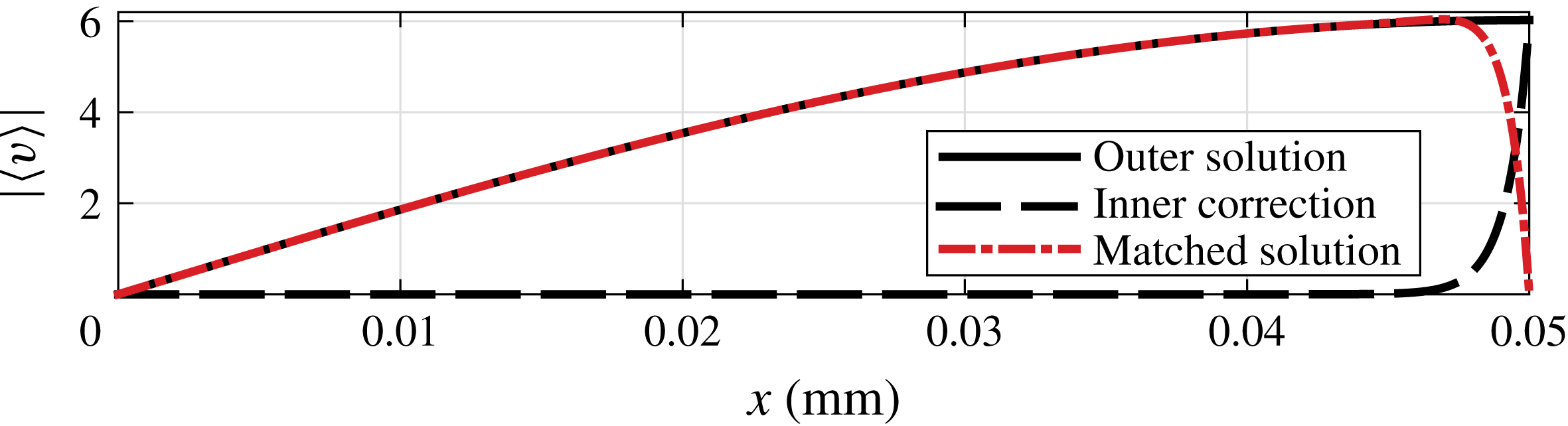
Example of the sidewall correction by an asymptotic matching technique for solution 1 and a forcing frequency equal to 2.6 Hz. The no-slip boundary condition at
 $x^{\prime }=l/2$
is satisfied by the matched solution
 $v+\bar{v}$
(dot-dashed line), which is given by adding the inner velocity correction (dashed line) to the vertical outer velocity
 $v$
(solid line).

The leading-order solution derived in § 3 does not satisfy the no-slip boundary condition at the lateral walls, thus suggesting that the scaling
 $x=x^{\prime }/\ell$
is not suited to describe the flow close to
 $x^{\prime }=\pm \ell /2$
. Let us here set
 $\bar{x}=(x^{\prime }\mp \ell /2)/\unicode[STIX]{x1D701}$
and look for an inner correction to the vertical velocity,
 $\bar{v}$
, such that the matched solution
 $v+\bar{v}$
tends to the outer solution,
 $v$
, far from the wall and satisfies the no-slip condition at
 $\bar{x}=0$
:
 $$\begin{eqnarray}\lim _{\bar{x}\rightarrow \infty }\bar{v}=0,\quad \bar{v}(\bar{x}=0,y,z)=-v\left(x=\pm {\textstyle \frac{1}{2}},y,z\right).\end{eqnarray}$$
At leading order, the inner velocity
 $\bar{v}$
obeys the Helmholtz equation
 $$\begin{eqnarray}\text{i}\bar{v}=\frac{1}{2}\unicode[STIX]{x1D6FF}^{2}\left(\frac{\unicode[STIX]{x2202}^{2}\bar{v}}{\unicode[STIX]{x2202}\bar{x}^{2}}+\frac{\unicode[STIX]{x2202}^{2}\bar{v}}{\unicode[STIX]{x2202}z^{2}}\right),\end{eqnarray}$$
which admits solutions of the kind
 $$\begin{eqnarray}\bar{v}(\bar{x},\bar{z})=\mathop{\sum }_{m=1}^{\infty }B_{m}(\bar{x})\sin [m\unicode[STIX]{x03C0}(z+1/2)],\end{eqnarray}$$
that satisfy the no-slip condition at
 $z=\pm 1/2$
. Substituting the Fourier series (A 3) in the governing equation (A 2) we get
 $$\begin{eqnarray}\frac{\text{d}^{2}B_{m}}{\text{d}\bar{x}^{2}}-\left(m^{2}\unicode[STIX]{x03C0}^{2}+\frac{2\text{i}}{\unicode[STIX]{x1D6FF}^{2}}\right)B_{m}=0\quad \Rightarrow \quad B_{m}(\bar{x})=B_{m}(0)\exp \left(-\bar{x}\sqrt{m^{2}\unicode[STIX]{x03C0}^{2}+\frac{2\text{i}}{\unicode[STIX]{x1D6FF}}}\right),\end{eqnarray}$$
where exponentially growing solutions have been discarded due to the first condition (A 1). In order to determine the unknown coefficients
 $B_{m}(0)$
, equation (A 3) is inserted in the no-slip condition (A 1). By projecting on the basis
 $\sin [m\unicode[STIX]{x03C0}(z+1/2)]$
and using (3.5) we obtain that
 $$\begin{eqnarray}\displaystyle B_{m}(0) & = & \displaystyle -2\int _{-1/2}^{1/2}v\left(\pm \frac{1}{2},y,z\right)\sin [m\unicode[STIX]{x03C0}(z+1/2)]\,\text{d}z\nonumber\\ \displaystyle & = & \displaystyle -\text{i}\frac{\unicode[STIX]{x2202}q}{\unicode[STIX]{x2202}y}\left(\pm \frac{1}{2},y,z\right)\frac{8\text{i}/\unicode[STIX]{x1D6FF}^{2}}{m\unicode[STIX]{x03C0}(m^{2}\unicode[STIX]{x03C0}^{2}+2\text{i}/\unicode[STIX]{x1D6FF}^{2})},\end{eqnarray}$$
if
 $m$
odd and
 $B_{m}(0)=0$
if
 $m$
even. Let define
 $m=2j+1$
with
 $j\in \mathbb{N}$
, whence the sidewall velocity correction is
 $$\begin{eqnarray}\bar{v}=\mathop{\sum }_{j=0}^{\infty }B_{2j+1}(0)\exp \left[-\bar{x}\sqrt{(2j+1)^{2}\unicode[STIX]{x03C0}^{2}+\frac{2\text{i}}{\unicode[STIX]{x1D6FF}}}\right]\sin [(2j+1)\unicode[STIX]{x03C0}(z+1/2)],\end{eqnarray}$$
and the matched velocity solution
 $v+\bar{v}$
satisfies the no-slip condition at
 $x^{\prime }=\ell /2$
, see figure 6. The outer and matched solutions are indistinguishable at
 $x_{g}=45$
mm.