2.1. Mortality forecasting

Mortality forecasting has seen significant advancements over the decades. The groundbreaking paper of Lee and Carter (Reference Lee and Carter1992) decomposed age-specific logarithmic mortality rates into components representing age patterns, a time trend modeled as a discrete-time stochastic process, and random noise, providing a flexible yet parsimonious framework for forecasting. Building on this foundation, Lee and Miller (Reference Lee and Miller2001) proposed the Lee–Miller variant to better fit historical data and improve forecast accuracy. Booth et al. (Reference Booth, Maindonald and Smith2002) further extended the LC framework with their Booth–Maindonald–Smith variant, incorporating age-specific improvements and adjustments for variable mortality decline. Meanwhile, Brouhns et al. (Reference Brouhns, Denuit and Vermunt2002) introduced a Poisson log-bilinear approach, integrating the LC methodology within a statistical framework that models death counts as Poisson-distributed variables, enabling rigorous probabilistic inference.

The Cairns–Blake–Dowd model (Cairns et al., Reference Cairns, Blake and Dowd2006) represented another significant contribution to the field, followed by several extensions in Cairns et al. (Reference Cairns, Blake, Dowd, Coughlan, Epstein, Ong and Balevich2009). This method focuses on higher ages and models the logit transform of death probabilities using stochastic processes for the intercept and slope parameters, making it particularly useful for pension and insurance applications.

Cohort effects are important extensions of these models, and the Age–Period–Cohort model (Clayton and Schifflers, Reference Clayton and Schifflers1987) is one of the foundational approaches in this field. It accounts separately for the effects of age, calendar time (period), and birth year (cohort) on mortality rates. Building on this, Renshaw and Haberman (Reference Renshaw and Haberman2006) proposed the Renshaw–Haberman model, which incorporates a cohort effect into the LC framework. The generalized age-period-cohort framework (Hunt and Blake, Reference Hunt and Blake2014), implemented by Villegas et al., (Reference Villegas, Kaishev and Millossovich2015), provides a unifying approach to modeling mortality and generalizes several models by incorporating a set of probability distributions and link functions, additional age–period interactions, and cohort effects.

P-spline smoothing, introduced by Currie et al. (Reference Currie, Durban and Eilers2004), is a flexible method for modeling and forecasting mortality rates while effectively balancing fit and smoothness, thereby capturing underlying trends while avoiding overfitting. Hyndman and Ullah (Reference Hyndman and Ullah2007) proposed a functional data approach to mortality forecasting, emphasizing robust handling of mortality and fertility rates by leveraging smooth functional representations of demographic data.

Multipopulation mortality forecasting has also been a topic of great interest. Li and Lee (Reference Li and Lee2005) extended the LC framework to handle groups of populations, ensuring coherent projections for related demographic units, such as neighboring countries or different sexes. Enchev et al. (Reference Enchev, Kleinow and Cairns2017) examined several multipopulation mortality models on data from England and Wales. Antonio et al. (Reference Antonio, Devriendt, de Boer, de Vries, De Waegenaere, Kan, Kromme, Ouburg, Schulteis, Slagter, van der Winden, van Iersel and Vellekoop2017) developed a stochastic multipopulation standard for Dutch and Belgian mortality projections. Lam and Wang (Reference Lam and Wang2023) introduced the weighted multivariate functional principal component approach for coherent multipopulation forecasting.

The LC model assumes constant rates of mortality improvement across ages, contrary to observed trends where mortality decline decelerates at younger ages and accelerates at older ages—a phenomenon known as the “rotation” of mortality decline. Li et al. (Reference Li, Lee and Gerland2013) incorporated this into the LC model for better long-term projections. Vékás (Reference Vékás2019) conducted an empirical analysis of this rotation in countries of the European Union using a new data-driven methodology, revealing the presence of this phenomenon in several member states, with notable differences between sexes.

Guibert et al. (Reference Guibert, Lopez and Piette2019) proposed penalized vector autoregression (VAR) to capture the dependence structure of mortality dynamics. Guibert et al. (Reference Guibert, Loisel, Lopez and Piette2020) presented locally coherent forecasts, which enforce coherence only in subgroups of countries and bridge the gap between the independence assumption of the LC model and the strict coherence enforced by the LL model. Li and Shi (Reference Li and Shi2021) introduced a global VAR approach that decomposes multipopulation mortality dynamics into local systems parsimoniously. Njenga and Sherris (Reference Njenga and Sherris2020) proposed Bayesian VAR as a related alternative. Jarner and Jallbjørn (Reference Jarner and Jallbjørn2020) discussed the application of cointegration for forecasting mortality factors. Li et al. (Reference Li, Tan, Tuljapurkar and Zhu2021) presented a multifactor mortality model based on the Gompertz law. He et al. (Reference He, Huang, Shi and Yang2021) introduced time-varying factor loadings into mortality forecasting models.

Recently, machine learning approaches, including neural network-based models, have significantly advanced mortality forecasting by accommodating the automatic detection of complex nonlinear dependencies (Hainaut, Reference Hainaut2018; Richman and Wüthrich, Reference Richman and Wüthrich2021; Perla et al., Reference Perla, Richman, Scognamiglio and Wüthrich2024, Reference Perla, Richman, Scognamiglio and Wüthrich2021; De Mori et al., Reference De Mori, Haberman, Millossovich and Zhu2025).

Comprehensive reviews of mortality forecasting methods and recent extensions are provided by Basellini et al. (Reference Basellini, Camarda and Booth2023) and Pascariu et al. (Reference Pascariu, Canudas-Romo and Vaupel2018), while Yao and Wang (Reference Yao and Wang2023) offer an overview of machine learning frameworks. A full survey of the mortality forecasting literature is beyond the scope of this paper.

2.2. Dynamic panel and spatiotemporal forecasting techniques

Pfeifer and Deutsch (Reference Pfeifer and Deutsch1980) introduced the spatiotemporal autoregressive moving average (STARMA) process as an extension of the well-known ARMA framework that is also capable of capturing spatiotemporal dependencies.

Arellano and Bond (Reference Arellano and Bond1991) popularized the generalized method of moments (GMM) estimator for dynamic panel linear models, and Blundell and Bond (Reference Blundell and Bond1998) introduced the improved system-GMM estimator. Yu et al. (Reference Yu, de Jong and Lee2008) presented the spatial dynamic panel model with fixed effects and investigated its asymptotic properties. Yu and Lee (Reference Yu and Lee2010) proposed a spatiotemporal dynamic panel model that works for both stationary and non-stationary data. Elhorst (Reference Elhorst2014) and Salima (Reference Salima2018) provided broad overviews of spatial panel models, and Astuti et al. (Reference Astuti, Setiawan and Purnomo2020) presented theoretical developments and potential research directions in this field.

Griffith (Reference Griffith2010, Reference Griffith2012) proposed eigenvector spatial filters and eigenvector spatiotemporal filters (ESTF) for modeling spatial and spatiotemporal relationships, and presented the contemporaneous and lagged spatiotemporal Moran’s I as two adequate measures of spatiotemporal autocorrelation in spatial panel data. Islam et al. (Reference Islam, Li, Lee and Wang2022) embedded this eigenvector approach into machine learning models.

2.3. Bayesian spatiotemporal mortality models

While Bayesian methods are not considered in our analysis, we include selected examples for context. Bayesian spatiotemporal mortality models (Ocaña-Riola and Mayoral-Cortés, Reference Ocaña-Riola and Mayoral-Cortés2010; Álvaro-Meca et al., Reference Álvaro-Meca2011; Greco and Scalone, Reference Greco and Scalone2013; Bennett et al., Reference Bennett, Li, Foreman, Best, Kontis, Pearson, Hambly and Ezzati2015; Gibbs et al., Reference Gibbs, Groendyke, Hartman and Richardson2020; Liu, Reference Liu2021) explicitly model structured spatiotemporal dependence through prior distributions. Hassan (Reference Hassan2021) extended the LC model using functional PCA, Ugarte et al. (Reference Ugarte, Goicoa and Militino2010) introduced Bayesian P-spline smoothing, Pickle (Reference Pickle2000) embedded spatiotemporal mortality forecasting in a linear mixed effects framework, and Carracedo et al. (Reference Carracedo, Debón and Iftimi2018) identified spatiotemporal mortality clusters in European data.

3.1. Spatial and spatiotemporal autocorrelation

Spatial autocorrelation refers to the correlation of a variable with itself across space—a manifestation of Tobler’s First Law of Geography (Tobler Reference Tobler1970). Moran’s I, introduced by Moran (Reference Moran1950), is a foundational statistic used to quantify global spatial autocorrelation, measuring the extent to which geographically proximate observations tend to exhibit similar (positive autocorrelation), dissimilar (negative autocorrelation) or spatially random (zero autocorrelation) values. The methodological foundations and theoretical properties of Moran’s I were significantly advanced by Cliff and Ord (Reference Cliff and Ord1973), establishing it as a core tool for exploratory spatial data analysis.

Given a set of N spatial observations $ \{u_i\}_{i=1}^N $ and an $ N\times N $ spatial weights matrix $ \textbf{W}_{\text{space}}\triangleq[w_{ij}] $ , Moran’s I is defined as:

\begin{equation*}I \triangleq \frac{N}{\sum_{i}\sum_{j} w_{ij}}\; \frac{\sum_{i}\sum_{j} w_{ij}(u_i - \bar{u})(u_j - \bar{u})}{\sum_{i}(u_i - \bar{u})^2},\end{equation*}

where $ \bar{u} $ is the mean of the observations, and $ w_{ij} $ encodes spatial relationships (e.g., contiguity weights, where $ w_{ij}=1 $ if regions i and j are neighbors and 0 otherwise, when values at neighboring locations are assumed to be autocorrelated; or inverse-distance weights, where $ w_{ij}=1/\delta_{ij} $ , when autocorrelation is assumed to decay with geographical distance $ \delta_{ij} $ measured between pairs of capital cities or centroids).Footnote 2

Local indicators of spatial association (LISA, Anselin, Reference Anselin1995) provide a standard framework for detecting spatial clustering and spatial outliers that may be obscured in global analyses. By decomposing the global Moran’s I statistic into contributions for each geographic unit, LISA identifies areas where neighboring values are significantly similar (high–high or low–low clusters) or dissimilar (high–low or low–high outliers). Statistical significance is typically assessed through permutation testing.

Spatiotemporal autocorrelation refers to the correlation of a variable with itself across space and time; in other words, it describes the similarity or dissimilarity of values measured at proximate locations and time points. In extending Moran’s I to spatiotemporal settings, the spatial weights matrix $ \textbf{W}_{\text{space}} $ is expanded using Kronecker products to form a spatiotemporal weights matrix $ \textbf{W}_{\text{space-time}} $ .

A common contemporaneous specification is given by:

\begin{equation*}\textbf{W}_{\text{space-time}}^{\text{(contemporaneous)}} \triangleq \textbf{I}_T \otimes \textbf{W}_{\text{space}} + \textbf{W}_{\text{time}} \otimes \textbf{I}_N,\end{equation*}

where $ \textbf{I}_T $ and $ \textbf{I}_N $ are identity matrices of size T and N, respectively, and $ \textbf{W}_{\text{time}} $ is a temporal adjacency matrix of size T connecting each time period with its predecessor and successor, with ones on the first lower and upper off-diagonals and zeros elsewhere (Griffith, Reference Griffith2010, Reference Griffith2012; Griffith and Paelinck, Reference Griffith and Paelinck2018).

Alternatively, the lagged specification is given by:

\begin{equation*}\textbf{W}_{\text{space-time}}^{\text{(lagged)}} \triangleq \textbf{W}_{\text{time}} \otimes \textbf{W}_{\text{space}} + \textbf{W}_{\text{time}} \otimes \textbf{I}_N,\end{equation*}

capturing the relationship between observations at each location and their neighbors’ past values.

Given these weights matrices, spatiotemporal Moran’s I is defined as:

\begin{align*}I^{\text{(spec)}}_{\text{space-time}} \triangleq \frac{NT}{\sum_{(i,t)}\sum_{(j,s)}w^{\text{(spec)}}_{(i,t),(j,s)}}\frac{\sum_{(i,t)}\sum_{(j,s)}w^{\text{(spec)}}_{(i,t),(j,s)}(u_{(i,t)}-\bar{u})(u_{(j,s)}-\bar{u})}{\sum_{(i,t)}(u_{(i,t)}-\bar{u})^2},\end{align*}

where $\text{spec} \in \text{\{contemporaneous,lagged\}} $ is the chosen specification, $ u_{(i,t)} $ denotes observations at location i and time t, and $ \bar{u} $ is the overall mean across all spatial and temporal observations (Griffith Reference Griffith2010).

It is both theoretically plausible and empirically supported to assume that mortality improvements exhibit spatiotemporal autocorrelation, thereby motivating the integration of spatiotemporal econometric methods into mortality forecasting.

3.2. Stochastic mortality models

Let $D_{xt}$ and $E_{xt}$ represent the number of deaths and the central exposure at age $x \in \mathcal{X}$ and year $\mbox{$t \in \{1,2,\ldots,T\}$}$ , where $\mathcal{X}$ denotes the age range included in the analysis, and let $m_{xt} \triangleq{D_{xt}}/{E_{xt}}$ be the corresponding central mortality rate. The LC model assumes

$$ \ln m_{xt} = a_{x} + b_{x}k_{t} + \varepsilon_{xt},$$

where $a_{x}$ and $b_{x}$ are age-specific parameters, $k_{t}$ is a time series, and $\varepsilon_{xt}$ are error terms with mean 0 and variance $\sigma_{\varepsilon}^{2}\gt0$ . For parameter estimation, we adopt the approach of maximizing the Poisson log-likelihood following Brouhns et al. (Reference Brouhns, Denuit and Vermunt2002), which provides a statistically rigorous alternative to the singular value decomposition (SVD) used by Lee and Carter (Reference Lee and Carter1992).

The parameters $a_x$ denote the average log-mortality rates by age in the sample, while the mortality index series $k_{t}$ represents mortality dynamics in the entire population, and $b_{x}$ determines sensitivities to changes in the mortality index by age group. To address the issue of identification, the following constraints are imposed:

$$\sum_{t=1}^T k_{t} = 0 \quad \text{ and }\quad \sum_{x \in \mathcal{X}} b_{x} = 1.$$

In the remainder of this paper, we will refer to country $i\in \{1,2,\ldots,N\}$ using an additional first subscript i in the notation of all parameters.

The LL model (Li and Lee, Reference Li and Lee2005) closely resembles the LC model in structure:

$$\ln m_{ixt} = a_{ix}+B_{x}K_{t}+b_{ix}k_{it}+ \varepsilon_{ixt},$$

where $B_{x}$ and $K_{t}$ are common parameters, $k_{it}$ , $b_{ix}$ , and $a_{ix}$ are population-specific parameters, and $\varepsilon_{ixt}$ are error terms, and it is assumed that

$$\sum_{t=1}^T K_t = \sum_{t=1}^T k_{it} = 0 \quad \text{and} \quad \sum_{x \in \mathcal{X}} B_{x}=\sum_{x \in \mathcal{X}} b_{ix} = 1 \quad (i=1,2,\ldots,N).$$

For the sake of coherent forecasts with

$$\lim_{t \rightarrow \infty}\frac{m_{ixt}}{m_{jxt}} = \text{constant} \quad (\forall x \in \mathcal{X},\; i \neq j),$$

all $k_{it}$ should converge to constants as $t\rightarrow\infty$ . Consequently, the authors advocate for employing AR(1) models with autoregressive coefficients less than 1 in absolute value or driftless random walk (RW) processes for forecasting the mortality indices $k_{it}$ .

3.3. Forecasting techniques

We consider the following forecasting techniques for the time series of the mortality indices $k_{i t}$ of the LC or LL models, with N and T denoting the number of countries and calendar years, respectively, and the notations $\boldsymbol{\xi}_t\triangleq(\xi_{1t}, \xi_{2t}, \ldots, \xi_{Nt})^{\intercal}$ $(t=1,2,\ldots,T)$ for the time-dependent and $\boldsymbol{\xi} \triangleq (\boldsymbol{\xi}_1, \boldsymbol{\xi}_2, \ldots, \boldsymbol{\xi}_T)^{\intercal}$ for the overall vector of innovations of the time series models with mean $\boldsymbol{\mu} \triangleq \mathbb{E}(\boldsymbol{\xi})$ and covariance matrix $\boldsymbol{\Sigma}\triangleq \mathbb{E}\left[(\boldsymbol{\xi}-\boldsymbol{\mu}) (\boldsymbol{\xi}-\boldsymbol{\mu})^{\intercal}\right]$ :

1. 1. Random walk with drift (RWD):

   $$\begin{aligned}k_{it}& =\alpha_i+k_{i,t-1}+\xi_{it},\\\boldsymbol{\xi} & \sim \mathcal{N}(\boldsymbol{\mu}, \boldsymbol{\Sigma}),\\\boldsymbol{\mu}&=\textbf{0}, \quad \boldsymbol{\Sigma}=\text{diag}(\sigma_1^2 \mathbf{I}_{T-1}, \sigma_2^2 \mathbf{I}_{T-1}, \ldots, \sigma_N^2 \mathbf{I}_{T-1}),\end{aligned}$$
   so that innovations are multivariate normal with mean zero, constant variance within countries, and no correlations across both countries and time periods. Assuming that the first-order differenced series is stationary, parameters can be estimated by maximum likelihood estimation (MLE). Lee and Carter (Reference Lee and Carter1992) used this specification for US data, and it has been shown to perform well across a large number of populations (Tuljapurkar et al., Reference Tuljapurkar, Li and Boe2000).

2. 2. Autoregressive integrated moving average (ARIMA):

   $$\begin{aligned} y_{it}&\triangleq\Delta^{\left(d_i\right)} k_{i t}=\alpha_i+\sum_{\ell=1}^{p_i} \phi_{i \ell} y_{i, t-\ell}+\sum_{\ell=1}^{q_i} \theta_{i \ell} \xi_{i, t-\ell}+\xi_{i t},\\\boldsymbol{\xi} & \sim \mathcal{N}(\boldsymbol{\mu}, \boldsymbol{\Sigma}),\\\boldsymbol{\mu}&=\textbf{0}, \quad \boldsymbol{\Sigma}=\text{diag}(\sigma_1^2 \mathbf{I}_{T-d_1}, \sigma_2^2 \mathbf{I}_{T-d_2}, \ldots, \sigma_N^2 \mathbf{I}_{T-d_N}).\end{aligned}$$
   Again, it is assumed that innovations are multivariate normal with mean zero, homoskedastic within countries and uncorrelated across countries and time periods. Differencing is applied to ensure the removal of unit roots for stationarity. As with RWD, the standard estimation method is MLE. The numbers of lags $p_i$ and $q_i$ by country can be optimized by minimizing the Bayesian information criterion (BIC) or related alternatives. The RWD is a special case with $p_i=0$ , $d_i=1$ , and $q_i=0$ $(i=1,2,\ldots,N)$ . There are no interactions among cross-sectional units.

3. 3. Dynamic panel linear model (DPLM):

   $$\begin{aligned}\textbf{y}_t&\triangleq\Delta^{(d)} \mathbf{k}_t=\boldsymbol{\alpha}+\sum_{\ell=1}^p \phi_{\ell} \mathbf{y}_{t-\ell}+\boldsymbol{\xi}_t,\\\boldsymbol{\mu}&=\textbf{0}, \quad \boldsymbol{\Sigma} = \text{diag}\left(\sigma_1^2 \mathbf{I}_{T-d}, \sigma_2^2 \mathbf{I}_{T-d}, \ldots, \sigma_N^2 \mathbf{I}_{T-d}\right)\!.\end{aligned}$$
   It is assumed that innovations have mean zero and are homoskedastic within countries and uncorrelated across countries and time periods. This in turn amounts to uniform ARIMA specifications with $d_i=d$ , $p_i=p$ , $\phi_{i\ell}=\phi_{\ell}$ , and $q_i=0$ $(i=1,2,\ldots,N$ ), but without the assumption of multivariate normality. Popular estimators for this model are the generalized method of moments (GMM, Arellano and Bond, Reference Arellano and Bond1991) and system-GMM (Blundell and Bond, Reference Blundell and Bond1998). The lag order p can be determined based on the statistical significance of the autoregressive terms. There are no interactions among cross-sectional units.

4. 4. Vector autoregression (VAR):

   $$\begin{aligned}\mathbf{y}_t&\triangleq\Delta^{(d)} \mathbf{k}_t=\boldsymbol{\alpha}+\sum_{\ell=1}^p \mathbf{A}_{\ell} \mathbf{y}_{t-\ell}+\boldsymbol{\xi}_t,\\\boldsymbol{\mu}&=\textbf{0}, \quad \boldsymbol{\Sigma} = \text{diag}\left(\sigma_1^2 \mathbf{I}_{T-d}, \sigma_2^2 \mathbf{I}_{T-d}, \ldots, \sigma_N^2 \mathbf{I}_{T-d}\right)\!.\end{aligned}$$
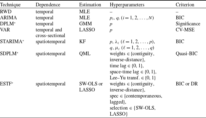
   Innovations are assumed to have mean zero and equal variance within countries, with no correlation across countries and time periods. Differencing ensures the removal of unit roots, as stationarity is required to fit the model. Estimation is typically performed by ordinary least squares (OLS), which does not require normality of the innovations. However, in our application, the ratio of observations to parameters is well below the commonly applied rule of thumb of at least five (Van Belle, Reference Van Belle2008), so OLS is not recommended. Instead, coefficients can be estimated using elastic net—or, as in our special case, LASSO or $L_1$ —regularization (Guibert et al., Reference Guibert, Lopez and Piette2019) in order to achieve a parsimonious description of the dependence structure. The lag order p can be determined by minimizing the cross-validated mean squared error (CV-MSE). The VAR framework allows for cross-sectional interactions, which are not necessarily spatial in nature.

5. 5. Spatiotemporal ARIMA (STARIMA, Pfeifer and Deutsch, Reference Pfeifer and Deutsch1980):

   $$\begin{aligned}z_{i t}& \triangleq \frac{\Delta^{\left(d\right)} k_{i t}-\underset{i,t}{\mathrm{mean}}\left(\Delta^{\left(d\right)} k_{i t}\right)}{\underset{i,t}{\mathrm{sd}}\left(\Delta^{\left(d\right)} k_{i t}\right)} =\\&=\alpha+\sum_{\ell=1}^p \sum_{r=0}^{\lambda_{\ell}} \phi_{\ell r} W^{(r)} z_{i, t-\ell}+\sum_{\ell=1}^q \sum_{r=0}^{\mu_{\ell}} \theta_{\ell r} W^{(r)} \xi_{i, t-\ell}+\xi_{i t}, \\\boldsymbol{\mu}&=\textbf{0}, \quad \boldsymbol{\Sigma} = \sigma^2 \mathbf{I}_{N(T-d)},\end{aligned}$$
   where $W^{(r)}$ is the r-th order spatial lag operator representing adjacency of r-th order.Footnote 3 Innovations are assumed to have mean 0 and equal variance across all countries, with no correlation across countries or time periods. Differencing ensures the removal of unit roots. Estimation is performed using the Kalman filter (KF), and the numbers of time lags p and q and space-time lags $\lambda_{\ell}$ $(\ell=1,2,\ldots,p)$ and $\mu_{\ell}$ $(\ell=1,2,\ldots,q)$ can be determined by minimizing the BIC. STARIMA is capable of capturing complex spatiotemporal interactions.

6. 6. Spatial dynamic panel linear model (SDPLM):

   $$\begin{aligned}\textbf{y}_t &\triangleq \Delta^{\left(d\right)} \mathbf{k}_t=\boldsymbol{\alpha}+\phi_{\text {space }} \textbf{W}_{\text{space}} \textbf{y}_t+\phi_{\text {time }} \textbf{y}_{t-1}+\phi_{\text {space-time }} \textbf{W}_{\text{space}} \textbf{y}_{t-1}+\boldsymbol{\xi}_t,\\\boldsymbol{\mu}&=\textbf{0}, \quad \boldsymbol{\Sigma} = \text{diag}\left(\sigma_1^2 \mathbf{I}_{T-d}, \sigma_2^2 \mathbf{I}_{T-d}, \ldots, \sigma_N^2 \mathbf{I}_{T-d}\right).\end{aligned}$$
   It is assumed that innovations have mean zero and are homoskedastic within countries and uncorrelated across countries and time periods. There is no normality assumption, and parameters are estimated by quasi maximum likelihood (QML), with the Lee–Yu transformation removing finite-sample bias (Yu and Lee, Reference Yu and Lee2010). The presence or absence of a time lag and a space-time lag, the choice between adjacency and inverse-distance spatial weights, and the necessity of the Lee–Yu transformation can be determined by minimizing the quasi-BIC. SDPLM allows for structured and easily interpretable spatiotemporal interactions.

7. 7. Eigenvector spatiotemporal filter (ESTF):

   $$\begin{aligned}\Delta^{\left(d\right)}\mathbf{k}_t&=\boldsymbol{\alpha}+\mathbf{S}_{\text {space-time }} \boldsymbol{\beta}+\mathbf{S}_{\text {space }} \boldsymbol{\gamma}+\mathbf{P} \boldsymbol{\phi}+\boldsymbol{\xi}_t,\\\boldsymbol{\mu}&=\textbf{0}, \quad \boldsymbol{\Sigma}=\text{diag}(\sigma_1^2 \mathbf{I}_{T-d}, \sigma_2^2 \mathbf{I}_{T-d}, \ldots, \sigma_N^2 \mathbf{I}_{T-d}),\end{aligned}$$
   where $\mathbf{S}_{\text{space}}$ and $\mathbf{S}_{\text {space-time}}$ are matrices of eigenvectors of the spatial and spatiotemporal weights matrices $\textbf{W}_{\text{space}}$ and $\mathbf{W}_{\text {space-time}}$ , and $\mathbf{P}$ is a matrix of country dummy variables. Griffith (Reference Griffith2010) proposes keeping all country dummy variables in the equation and using stepwise OLS (SW-OLS) estimation for the sake of parsimony, or alternatively, shrinkage by LASSO can be applied.Footnote 4 Choices between adjacency and inverse-distance spatial weights and between contemporaneous and lagged specifications can be made by minimizing the BIC in the case of SW-OLS and the deviance ratio (DR) in the case of LASSO. ESTF allows for complex spatiotemporal interactions, but is typically less interpretable than an SDPLM.

Chief properties of the proposed techniques are displayed in Table 1. Additionally, we consider two ensemble techniques. The first one, denoted by ENS1, computes the mean predicted log-mortality rate across the seven forecasting techniques for every country, age, and calendar year in both the LC and LL models, whereas the second one, denoted by ENS2, computes a trimmed mean excluding the lowest and highest predictions.

Table 1.

Properties of the various techniques (^*: not used previously in this context).

Given the time series $ k_{it} $ for each country from the LC model, univariate unit root and second-generation panel unit root tests (Hurlin and Mignon, Reference Hurlin and Mignon2007) may help determine their orders of integration. The latter account for cross-sectional dependence, which is central to our approach. Specifically, for ARIMA, we use augmented Dickey–Fuller (ADF) tests to determine country-specific orders $ d_i $ such that the differenced series have no unit roots. For all forecasting techniques other than RWD and ARIMA, we use the covariate-augmented Dickey–Fuller (CADF) test (Costantini and Lupi, Reference Costantini and Lupi2013), a second-generation panel unit root test, to determine a uniform order of integration $ d_i=d $ $ (i=1,2,\ldots,N) $ across countries.

For the LL model, following Li and Lee (Reference Li and Lee2005), we recommend forecasting the common trend $K_t$ using an RWD process estimated by MLE. For the country-specific $k_{it}$ , we set $d_i = 0$ and $d = 0$ across all countries and forecasting techniques to ensure coherence.

In the remainder of our paper, we will use the word “model” for the LC and LL models, and “technique” for the forecasting techniques presented in this subsection.Footnote 5

3.4. Robust selectionFootnote ⁶

We propose dividing the dataset into a training set, consisting of the initial $ T_{\text{train}} $ years of available data, and a test set, comprising the remaining $ T_{\text{test}} $ years, with $ T = T_{\text{train}} + T_{\text{test}} $ , thereby spanning the entire observation period. Additionally, because model performance may be sensitive to the location of the train–test split, we propose a robust selection procedure involving repeated estimation across multiple training horizons $ T_{\text{train}}^{(h)} $ , with 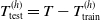$T^{(h)}_{\text{test}}=T-T^{(h)}_{\text{train}}$ $(h=1,2,\ldots,H)$ .

Forecast accuracy of forecasting technique j under model $\ell$ (LC or LL in our case) in country i given train–test split h is then evaluated using the mean squared error (MSE) of the forecasted logarithmic mortality rates:

\[\text{MSE}^{(h)}_{i,j,\ell} \triangleq\frac{1}{X T^{(h)}_{\text{test}}} \sum_{x \in \mathcal{X}} \sum_{t = T^{(h)}_{\text{train}} + 1}^{T} \left( \ln m_{ixt} - \ln \hat{m}^{(j,\ell)}_{ixt} \right)^2,\]

where $\hat{m}^{(j,\ell)}_{(\cdot)}$ denotes mortality rates forecasted using technique j with its optimal hyperparameters under model $\ell$ .

As it is preferable to assess model performance relative to the best-performing procedure rather than against a perfect fit or another hypothetical benchmark, for each split, we define the underperformance scores

\[\text{U}^{(h)}_{i,j,\ell} \triangleq\text{MSE}^{(h)}_{i,j,\ell} - \min_{j,\ell} \text{MSE}^{(h)}_{i,j,\ell},\]

which measure how much worse forecasting technique j under model $\ell$ performs for country i and training horizon h, relative to the best-performing combination.

Model underperformance can then be assessed independently from the location of the train–test split by measuring average or maximum underperformance (AU or MU) scores across the splits, with the maximum criterion being more conservative and reflecting the minimax principle from decision theory:

\begin{align*}\text{AU}_{i,j,\ell} &\triangleq \frac{1}{H}\sum_{h=1}^H \text{U}^{(h)}_{i,j,\ell},\\[5pt]\text{MU}_{i,j,\ell} &\triangleq \max_{h=1,2,\ldots,H} \text{U}^{(h)}_{i,j,\ell}.\end{align*}

These measures can then be summarized by their medians across all countries, enabling the robust comparison of model–technique combinations:

\begin{align*}\text{MAU}_{j,\ell} &\triangleq \underset{i=1,2,\ldots,N}{\text{median}}(\text{AU}_{i,j,\ell}),\\[5pt]\text{MMU}_{j,\ell} &\triangleq \underset{i=1,2,\ldots,N}{\text{median}}(\text{MU}_{i,j,\ell})\end{align*}

MAU captures median average underperformance relative to the best-performing combination, while MMU reflects median worst-case underperformance across train–test splits.

3.5. Stochastic forecasts

Stochastic forecasts may be generated by incorporating some or all of the following four sources of uncertainty (Cairns Reference Cairns2000):

1. 1. Measurement uncertainty arises from the random error terms $\varepsilon_{ixt}$ in the LC and LL log-mortality equations. It captures fluctuations in observed log-mortality rates that are not explained by the systematic components of the models.

2. 2. Process uncertainty arises from the inherent randomness in the future evolution of the stochastic time series components $k_{it}$ of the models.

3. 3. Parameter uncertainty results from potential errors in the estimation of the model parameters $a_{ix}$ , $b_{ix}$ , $ k_{it} $ , $B_x$ , and $K_t$ based on finite historical data.

4. 4. Model uncertainty reflects the possibility that the chosen model structure (e.g., LC–RWD) may be misspecified, or that alternative models could better represent the underlying mortality dynamics.

Following the approach recommended by Brouhns et al. (Reference Brouhns, Denuit and Keilegom2005), we address parameter uncertainty by generating synthetic training datasets of bootstrapped death counts $\{D^{(r)}_{ixt}\}_{r=1}^{R}$ drawn independently from Poisson distributions with means $\lambda_{ixt} \triangleq D_{ixt}$ , where R is the number of bootstrap samples. This yields bootstrapped estimates $a^{(r)}_{ix}$ , $b^{(r)}_{ix}$ , and $k^{(r)}_{it}$ separately for the LC and LL models and $B^{(r)}_x$ and $K^{(r)}_t$ for the LL model.

We incorporate process uncertainty via resampling with replacement from the past residuals of the fitted time series model for the given country:Footnote 7

\begin{align*}\Delta^{(d_i)} k^{(r)}_{i, T_{\text{train}}+t} &= \Psi^{(r)}_{it} + \xi^{(r)}_{it} \quad (t \geq 1,\ r = 1,2,\ldots,R),\end{align*}

and additionally, for the LL model, we apply

\begin{align*}\Delta K^{(r)}_{T_{\text{train}}+t} &= \Theta^{(r)}+\eta_t^{(r)}\quad (t \geq 1,\ r = 1,2,\ldots,R),\end{align*}

where $\Psi^{(r)}_{it} \triangleq \mathbb{E}_{T_{\text{train}}}\left(\Delta^{(d_i)} k^{(r)}_{i,T_{\text{train}}+t}\right)$ with $\mathbb{E}_{T_{\text{train}}}(\!\cdot\!)$ denoting a conditional expectationFootnote 8 based on bootstrapped samples up to $T_{\text{train}}$ , $\Theta^{(r)}$ is the drift term of the RWD process of the common mortality index $K_t$ , and $\xi^{(r)}_{it}$ and $\eta^{(r)}_{t}$ are randomly drawn with replacement from training-set residuals of $\Delta^{(d_i)}k_{it}$ and $\Delta K_t$ $(t=1,2,\ldots,T_{\text{train}})$ . We draw from the residuals rather than from normal distributions, as the normality assumption may not hold and methods outside the ARIMA family do not rely on it.

We account for measurement uncertainty by adding bootstrapped residuals $\varepsilon^{(r)}_{i,x,T_{\text{train}}+t}$ drawn from past values $\{\hat{\varepsilon}_{ixt}\}_{t=1}^{T_{\text{train}}}$ to the systematic components of the log-mortality equations (with $B^{(r)}_x\triangleq K^{(r)}_t\triangleq0$ in the case of the LC model):

\[\ln m^{(r)}_{i,x,T_{\text{train}}+t} \triangleq \ln m^{(r)}_{i,x,T_{\text{train}}} + b^{(r)}_{ix}(k^{(r)}_{i,T_{\text{train}}+t}-k^{(r)}_{i,T_{\text{train}}})+B^{(r)}_x(K^{(r)}_{T_{\text{train}}+t}-K^{(r)}_{T_{\text{train}}})+\varepsilon^{(r)}_{i,x,T_{\text{train}}+t}.\]

Model uncertainty could be accounted for within a fully Bayesian framework; however, we leave this aspect outside the scope of the present study, as subjective priors would introduce a new layer of uncertainty, and model averaging with BIC-derived weights is not feasible as some forecasting techniques we have proposed are not estimated by maximum likelihood. Instead, we apply post hoc adjustment and ensembling to mitigate this limitation.

To reduce sampling bias, we apply mean calibration, that is, a pointwise shift to the bootstrapped trajectories so that their sample mean equals the expected trajectory $\hat{m}_{i,x,T_{\text{train}}+t}$ computed under the given model–technique combination at the end of the training period:

\[\ln \tilde{m}^{(r)}_{i,x,T_{\text{train}}+t} \triangleq \ln m^{(r)}_{i,x,T_{\text{train}}+t} + \ln \hat{m}_{i,x,T_{\text{train}}+t} - \frac{1}{R}\sum_{r=1}^R \ln m^{(r)}_{i,x,T_{\text{train}}+t}.\]

Then, we construct bootstrapped prediction intervals with confidence level $1-\tau$ for the log-mortality rates $\ln m_{i,x, T_{\text{train}}+t}$ as

\[\left( \pi^{(L, \tau)}_{i,x,T_{\text{train}}+t}, \pi_{i,x,T_{\text{train}}+t}^{(U, \tau)} \right) \triangleq \left(Q_{\frac{\tau}{2}}\left(\{\ln \tilde{m}^{(r)}_{i,x,T_{\text{train}}+t}\}_{r=1}^R\right),\quad Q_{1-\frac{\tau}{2}}\left(\{\ln \tilde{m}^{(r)}_{i,x,T_{\text{train}}+t}\}_{r=1}^R\right)\right)\!,\]

where $Q_{\tau}(\!\cdot\!)$ denotes the empirical $\tau$ -quantile of the resampled estimates.

To correct potentially inaccurate interval coverage (e.g., due to model uncertainty or structural breaks), we apply a post hoc scaling adjustment by solving for scaling factors $ \nu_t $ that achieve the empirical nominal coverage probability $ 1-\tau $ on a validation set of length $ T_{\text{val}} $ , for each model–technique combination and forecast horizon $ t=1,2,\ldots, T_{\text{val}} $ :

where are indicator functions, and

\begin{align*}\left( \pi^{*(L,\tau)}_{i,x,T_{\text{train}+t}}, \pi^{*(U,\tau)}_{i,x,T_{\text{train}+t}}\right)\triangleq\Big( \pi^{(L,\tau)}_{i,x,T_{\text{train}+t}} - \frac{\nu_t - 1}{2} \left( \pi^{(U,\tau)}_{i,x,T_{\text{train}}+t} - \pi^{(L,\tau)}_{i,x,T_{\text{train}}+t} \right), \\[8pt] \nonumber \pi^{(U,\tau)}_{i,x,T_{\text{train}}+t} + \frac{\nu_t - 1}{2} \left( \pi^{(U,\tau)}_{i,x,T_{\text{train}}+t} - \pi^{(L,\tau)}_{i,x,T_{\text{train}}+t} \right)\Big).\end{align*}

We assess the quality of these prediction intervals on a separate evaluation period of length $T_{\text{eval}}$ , with the original test period partitioned as $T_{\text{val}}+T_{\text{eval}}=T_{\text{test}}$ , using average interval scores (Gneiting and Raftery, Reference Gneiting and Raftery2007) by country, computed as

\begin{align*}\text{AIS}_{i, 1-\tau} & \triangleq \frac{1}{\left|\mathcal{X}\right| \, T_{\text{eval}}} \sum_{x \in \mathcal{X}} \sum_{t=1}^{T_{\text{eval}}}\Big[ \pi^{*(U,\tau)}_{i,x,T_{\text{train}}+T_{\text{val}}+t} - \pi^{*(L,\tau)}_{i,x,T_{\text{train}}+T_{\text{val}}+t}\Big.\\&\quad\left.+\frac{2}{\tau} \max\Big(\pi^{*(L,\tau)}_{i,x,T_{\text{train}}+T_{\text{val}+t}} - \ln m_{i,x,T_{\text{train}}+T_{\text{val}+t}}, 0\Big)\right.\\&\quad +\frac{2}{\tau} \max\Big(\ln m_{i,x,T_{\text{train}}+T_{\text{val}+t}} - \pi^{*(U,\tau)}_{i,x,T_{\text{train}}+T_{\text{val}+t}}, 0\Big)\Big] ,\end{align*}

where we sample from the first $T_{\text{train}}+T_{\text{val}}$ years, simulate for the remaining $T_{\text{eval}}$ years, use mean calibration to expected trajectories estimated at the end of the validation period, and apply the scaling factors $\nu_t$ previously estimated on the validation period.

Finally, we compute median average interval scores across countries as a robust summary of prediction interval quality across model–technique combinations:

\begin{align*} \text{MAIS}_{1-\tau}\triangleq \underset{i=1,2,\ldots,N}{\text{median }} \text{AIS}_{i, 1-\tau},\end{align*}

and assess out-of-sample coverage using empirical coverage probabilities:

This procedure could be made even more robust by using multiple train–test splits, following the analogy of the robust selection pipeline described in Subsection 3.4.

Figure 1.

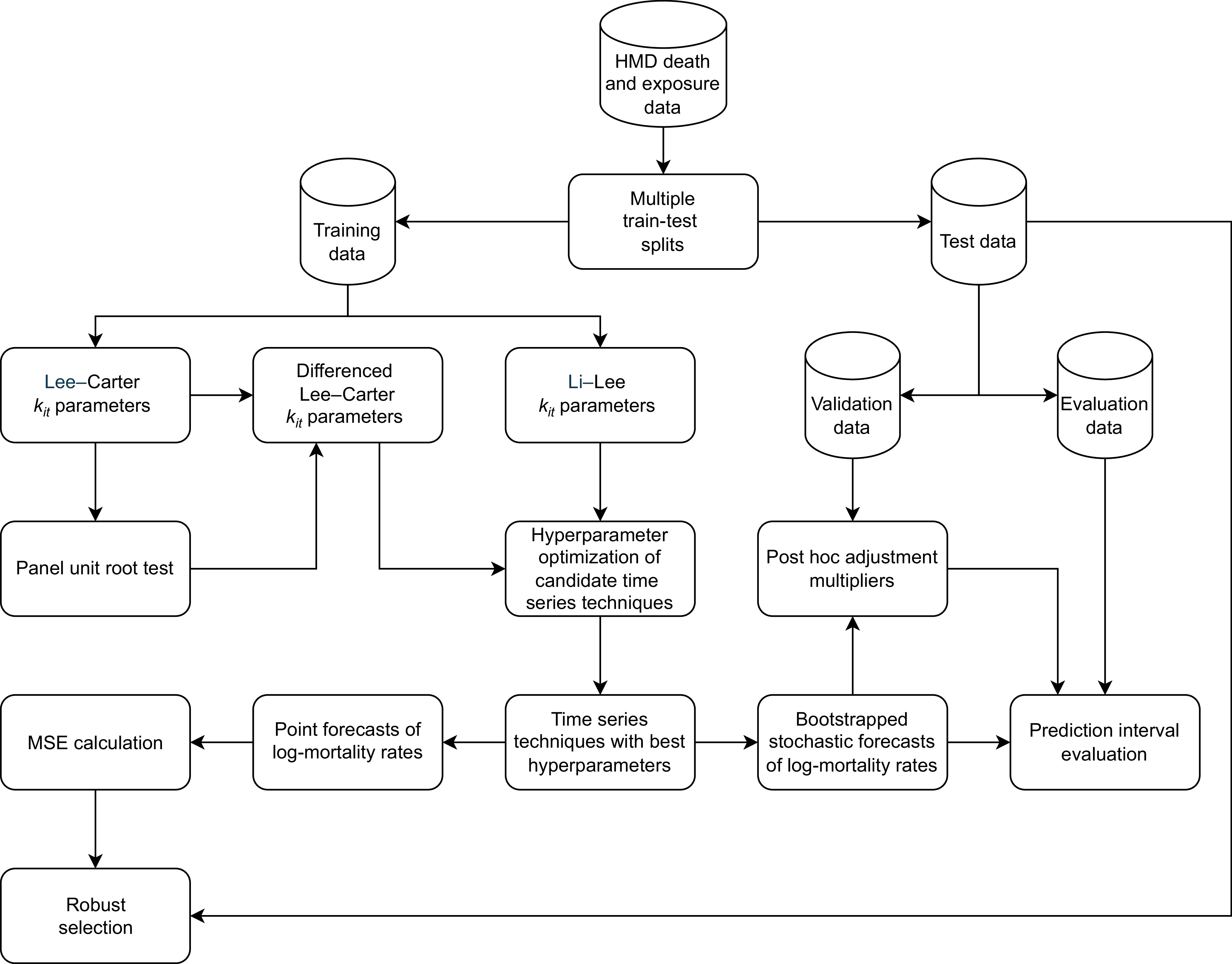
Analysis workflow.

4.1. Data collection and preparation

We obtained our dataset from the Human Mortality Database (HMD, 2025). We collected unisex data on the number of deaths and exposures in all European countries for which data were available for the $T=60$ years between 1960 and 2019, categorized by country, age, and calendar year, and excluded the remaining countries. We did not use data for ages above 99 years due to missing data and other potential data quality issues. Consequently, our dataset comprised the $N=22$ countries depicted in Figure 2.

Figure 2.

Map of the countries included in the analysis with their ISO-2 codes.

We used data only up to 2019 to avoid testing on the years of the COVID-19 pandemic, which would have led to a bias toward models that tend to overestimate mortality. Assuming that COVID-19 was a one-off event, the pandemic years could be included after subtracting COVID-19 deaths from total counts or by interpolating data for the years of the pandemic using rates from neighboring years. However, a significant problem with the subtraction approach is that criteria for recording the cause of death and the extent of testing varied widely by country, while the second approach is not yet viable as data for years following the end of the pandemic are not yet available for some countries in the Human Mortality Database. Due to these constraints, we opted to perform our analysis on this truncated period.

By default, we used the first $T_{\text{train}} = 45$ years, up to 2004, as training data, the remaining $T_{\text{test}} = 15$ years as test data, and split the test period into a validation period of $T_{\text{val}}=8$ years and an evaluation period of $T_{\text{eval}}=7$ years.

4.2. Model estimation and interpretation

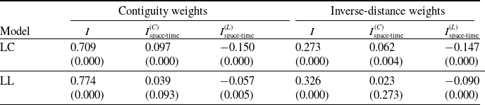
We estimated the parameters of the LC and LL models on data from all $N=22$ countries. Table 2 displays the spatial and spatiotemporal Moran’s I statistics of the differenced mortality indices $\Delta k_{it}$ of the LC and LL models using contiguity and inverse-distance spatial weightsFootnote 10. These results indicate that there is significant spatial and spatiotemporal autocorrelation in mortality improvements in both the LC and LL models, which motivates the application of spatiotemporal forecasting techniques, and contiguity weighting yields stronger spatiotemporal autocorrelation than inverse-distance weighting.

We performed LISA clustering at the 5% significance level on the means of $\Delta k_{it }$ from the LC and LL models by country. We used contiguity weighting in this step, based on the findings reported in Table 2. LISA identified two spatial clusters for the LC model: France and Switzerland and the Baltic states of Estonia, Latvia, and Lithuania, both showing high mean differences in the mortality index. For the LL model, the first significant cluster consisted of France and Germany, and the second of the three Baltic states, again both with high mean differences.

In the ESTFs, the spatiotemporal eigenvectors with the largest absolute coefficients revealed clear spatial patterns. In the LC model, they separated the United Kingdom and Ireland, as well as the Scandinavian countries of Finland, Norway, and Sweden, from the rest of Europe under both Stepwise and LASSO selections. In the LL model, they again isolated these same clusters under LASSO, while under stepwise the three Baltic states were separated from the rest of Europe. This has a natural geographic interpretation, as the separated groups of countries are divided by bodies of water from the rest of the countries in the analysis.

Table 2.

Spatial and spatiotemporal Moran’s I statistics of the differenced mortality indices $\Delta k_{it}$ from the LC and LL models under alternative spatial weighting schemes (p-values in parentheses).

4.3. Forecasting techniques and hyperparameter optimization

We assessed the stationarity of the LC mortality indices using the CADF test, which yielded the p-values $0.847$ on the original panel data and $0.000$ after differencing, indicating the successful removal of unit roots, and $d=1$ as the uniform order of integration.

For both the LC and LL models, we estimated the parameters and optimized the hyperparameters of the time series forecasting techniques as we outlined in Table 1. In all cases, the contiguity spatial weights matrix outperformed the version constructed from inverse distances between capital cities, in line with the findings from Table 2.

4.4. Point forecasts

We forecasted the country-specific mortality indices of the LC and LL models and the log-mortality rates using all forecasting techniques presented in Subsection 3.3, each with its optimal set of hyperparameters, using observed jump-off rates to enhance forecast accuracy, as recommended by Lee and Miller (Reference Lee and Miller2001), and applied an RWD for the common mortality index of the LL modelFootnote 11 The first row of Figure 3 illustrates the LC model predictions for Norway across selected ages, and the second row shows the corresponding coherent LL forecasts.Footnote 12

4.5. Robust selection

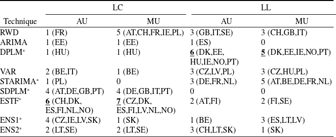
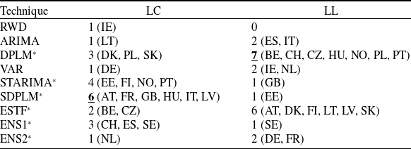
Following forecasting, we applied the robust selection procedure described in Subsection 3.4, using the years 2001 through 2007 as the endpoints of the training period (i.e., $T_{\text{train}} \in \{42, 43, 44, 45, 46, 47, 48\}$ ) to evaluate the predictive performance of the combinations of the LC and LL models and the seven forecasting techniques and the two ensembles. The numbers and ISO-2 codes of the countries in which each technique performs best under each model, based on AU and MU, are summarized in Table 3.Footnote 13

Table 3.

Number of wins by technique within each model, and ISO-2 codes of countries where they won, based on AU and MU. Asterisks denote newly proposed techniques in this context, and highest win counts by column are typeset in bold underlined font.

Figure 3.

Point projections of log-mortality for selected ages in Norway from the LC (first row) and LL (second row) models.

Within the LC framework, LC–ESTF emerges as the strongest overall performer, with 6 and 7 wins under AU and MU, respectively. LC–SDPLM also performs well, achieving 4 wins under both criteria. Overall, the spatiotemporal techniques account for 17 and 14 wins under AU and MU, respectively, out of the 22 populations.

Within the LL model, LL–DPLM stands out with 6 and 5 wins under AU and MU, respectively, making it the best performer across criteria. LL–STARIMA follows with 3 and 5 wins. Spatiotemporal techniques are best in 9 and 11 countries under AU and MU, respectively—less frequently than in the LC framework. This is expected, as the common trend in the LL model already captures much of the cross-country dependence, and the spatiotemporal techniques can only leverage residual dependence beyond this.

Spatiotemporal techniques often outperform generic VAR as they rely on more parsimonious dependence structures.

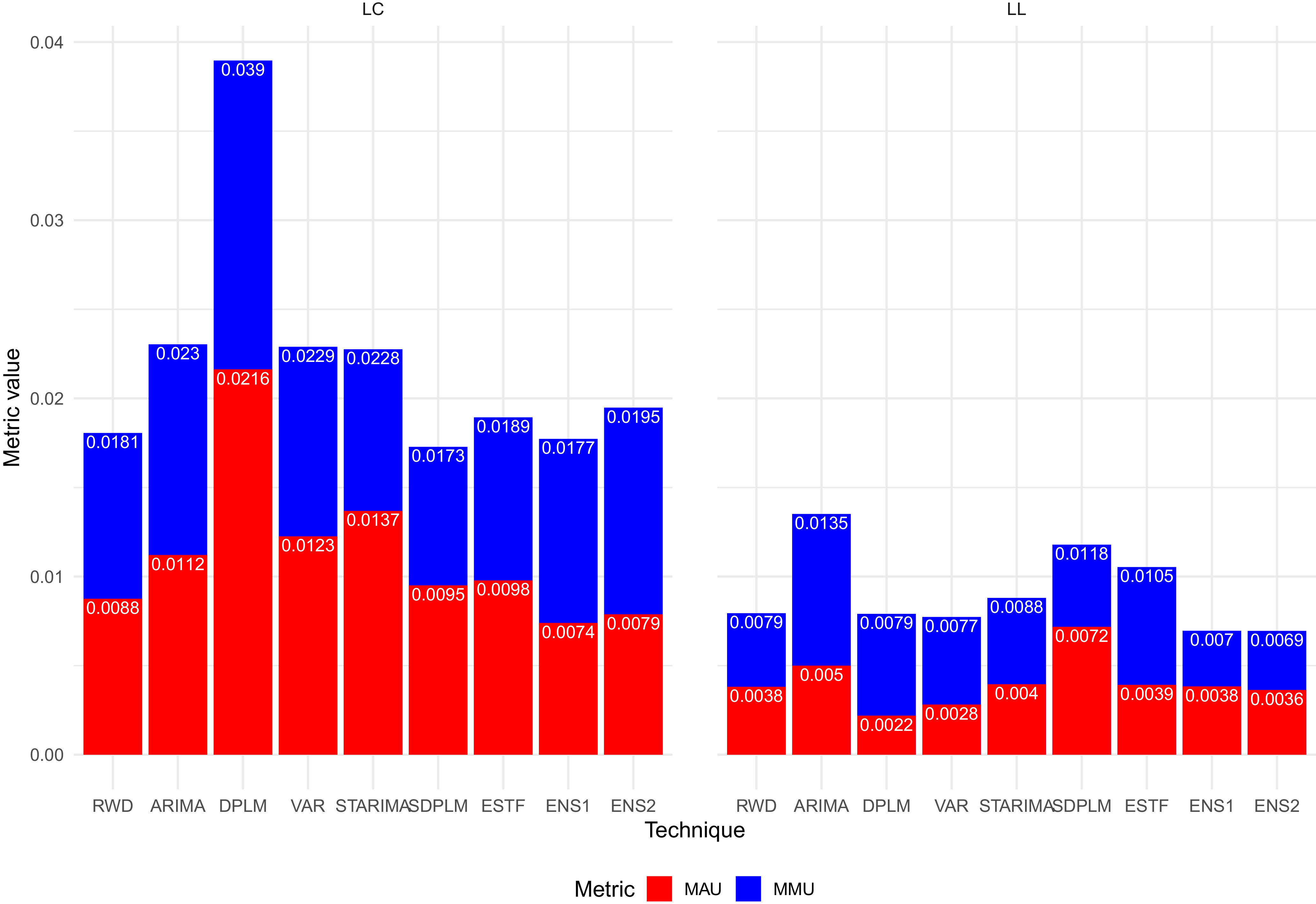
We provide another comprehensive summary of our results in Figure 4, where the red bars display MAU, the red and blue bars combined correspond to values of the more cautious MMU, and the left and right panels refer to the LC and LL models, respectively. This comparison is chiefly relevant if the same model–technique combination is applied in all countries. Otherwise, country-specific combinations are clearly superior.

Figure 4.

Comparison of MAU and MMU values across models and techniques (MMU is the sum of the heights of the red and blue columns).

As shown in Figure 4, the LL–DPLM model achieves the lowest overall MAU, but is slightly outperformed by the ensembles LL–ENS1 and LL–ENS2 in terms of the more conservative MMU. Within the LC model, the ensembles LC–ENS1 and LC–ENS2 achieve the lowest MAU, while LC–SDPLM is the best in terms of MMU.

Notably, ensembles achieve excellent overall MAU and MMU, and LL-based forecasts outperform LC-based ones, as they incorporate information on the common trend distilled from a larger set of data in addition to country-specific patterns, while remaining coherent.

Overall, on the set of countries, ages and calendar years under consideration, LL–DPLM, LC–ESTF, LL–VAR, and LL–STARIMA emerge as strong performers, with notable variation by country. The widely used RWD and ARIMA specifications are clearly outperformed by other procedures in both the LC and LL frameworks.

4.6. Stochastic forecasts

We performed the procedure presented in Subsection 3.5 using $T_{\text{train}}=45$ , $T_{\text{val}}=8$ , and $T_{\text{eval}}=7$ years, $R=100$ bootstrap samples, and a confidence level of $1-\tau=0.9$ . For the sake of illustration, the first and second rows of Figure 5 display mean-calibrated, post hoc adjusted, bootstrapped 90% prediction intervals of log-mortality rates for selected ages in Norway, based on the LC–ESTF and LL–ESTF frameworks.Footnote 14

Table 4.

Number of countries in which each forecasting technique yields the lowest average 90% interval score, and ISO-2 codes of countries where they won. Asterisks denote newly proposed techniques, and highest win counts by model are typeset in bold underlined font.

Figure 5.

Bootstrapped 90% prediction intervals for selected ages in Norway from the LC–ESTF (first row) and LL–ESTF (second row) frameworks.

As ENS1 and ENS2 lack their own mortality index series, we computed their prediction intervals as quantiles of the means and trimmed means, respectively, of the bootstrapped samples of the log-mortality rates from the seven individual techniques and applied all subsequent modeling steps in the same way as to the original techniques.

Table 4 reports the number and list of countries in which each technique achieves the lowest average 90% interval score under the LC and LL models. Under LC, SDPLM performs best, winning in six countries, followed by STARIMA, DPLM and ENS1, while the classical benchmarks RWD and ARIMA win in one country each. Under LL, DPLM attains the highest number of wins (seven), closely followed by ESTF (six), whereas ARIMA wins in only two countries and RWD in none.

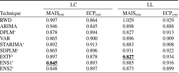
Table 5 reports median average 90% interval scores and empirical coverage probabilities across forecasting techniques. Under the LC model, ENS1 achieves the lowest median interval score, closely followed by ENS2 and SDPLM, while classical benchmarks exhibit higher scores. Under the LL model, ESTF attains the lowest MAIS, with DPLM performing similarly well. Empirical coverage probabilities are generally close to the nominal level across methods, while LL-based frameworks tend to slightly overcover.

Table 5.

Median average 90% interval scores and empirical coverage probabilities by forecasting technique under the LC and LL models. Asterisks denote newly proposed techniques, and lowest MAIS by model are typeset in bold underlined font.

4.7. Robustness check

To assess the robustness of our forecasts, we compared period life expectancy at birth at the end of the test period in 2019, computed using the various forecasting techniques estimated on the training period 1950–2004, for all $N=22$ countries and both the LC and LL models. This choice was motivated by four considerations: (i) life expectancy at birth is an easily interpretable measure with an intuitive scale; (ii) it summarizes mortality across all ages into a single indicator, allowing for a parsimonious comparison; (iii) by the end of the test period, forecasts from different techniques are expected to have diverged sufficiently to allow for an informative comparison; and (iv) unlike cohort life expectancies, it does not require re-estimating the models and techniques on the full dataset and forecasting an additional 100 years, which would be more speculative as well as computationally demanding.

By careful individual examination of the projected mortality trajectories by country, model, and technique, we identified a few anomalies. In the Baltic states of Estonia, Latvia, and Lithuania, the LC mortality index series $k_{it}$ increases over time, accompanied by negative values of $b_{ix}$ at childhood and some other ages and positive values at middle ages. This pattern captures the idiosyncratic mortality experience of these countries, where middle-aged mortality stagnated or worsened during the late Soviet period (Krúmiņš and Zvidriņš Reference Krúminš and Zvidrinš1992), while other age groups experienced improving mortality. STARIMA introduces decreases into $k_{it}$ over several periods, which leads to projected increases in child mortality and decreases in middle-aged mortality in the forecasts for all three countries. A similar inversion is observed for ESTF in Estonia and Latvia. As this behavior is clearly a modeling artifact, we exclude LC–STARIMA for all three countries and LC–ESTF for Estonia and Latvia. This inversion does not affect the robust selection or the evaluation of prediction intervals presented in Subsections 4.5 and 4.6, as these techniques were not selected for the affected countries and the reported medians are robust to outliers.

The results are displayed in Figure 6, which shows little variation across techniques. The standard deviations across techniques, computed separately for each country and model, range from 0.01 to 1.06 years, with a median of 0.44 years, corroborating the robustness of our forecasts.