


1. Introduction
The trailing vortex has been one of the major concerns in fluid dynamics because of the danger imposed on following aircraft owing to its long lifespan, known as the wake-encounter problem. One way to alleviate the impact of the trailing vortex is to accelerate the path to vortex breakdown through the manipulation of its inherent instabilities (Spalart Reference Spalart1998; Gerz, Holzäpfel & Darracq Reference Gerz, Holzäpfel and Darracq2002). Consequently, such a need calls for a greater understanding of the inherent instabilities of the trailing vortex to guide the design of physics-based flow control strategies.
In hydrodynamic stability problems, one of the major concerns is to determine the perturbation modes associated with the instabilities of a certain flow of interest. In these quests, two perspectives on the evolution of perturbations have been receiving most attention, namely the transient instability and asymptotic instability. The transient perspective focuses on the short-term behaviour of perturbations where both the primary and secondary modes take effect; while in the asymptotic limit, only the primary mode survives as time progresses. For a trailing vortex, the transient instability has been investigated in detail by Antkowiak & Brancher (Reference Antkowiak and Brancher2004), Pradeep & Hussain (Reference Pradeep and Hussain2006), Heaton (Reference Heaton2007a), Brion, Sipp & Jacquin (Reference Brion, Sipp and Jacquin2007) and Navrose et al. (Reference Navrose, Johnson, Brion, Jacquin and Robinet2018), and the dominating asymptotic perturbations have been revealed both at the inviscid limit and with viscosity (Lessen & Paillet Reference Lessen and Paillet1974; Lessen, Singh & Paillet Reference Lessen, Singh and Paillet1974; Mayer & Powell Reference Mayer and Powell1992; Fabre & Jacquin Reference Fabre and Jacquin2004). While the transient growth of instability can be attributed to the non-normality of eigenvectors of the Navier–Stokes (N–S) operator (Chomaz Reference Chomaz2005; Schmid Reference Schmid2007), the mechanism underlying the asymptotic instability is intriguing, that is, why one particular perturbation undergoes asymptotic growth or decay in the flow of the leading order.
1.1. Characteristics of asymptotic instability for trailing vortices
The instabilities of an isolated trailing vortex has been receiving considerable attention, as such a vortex resembles a typical wing-tip vortex in the far-field. In practice, the isolated vortex is often modelled as a  $q$-vortex derived from Batchelor's solution of the incompressible N–S equation (Batchelor Reference Batchelor1964). The stability of an isolated vortex can be generally classified into two categories: inviscid and viscous. Research on inviscid stability can be dated back to Lessen et al. (Reference Lessen, Singh and Paillet1974). In their work, helical modes with a negative azimuthal wavenumber
 $m$, which counter the vortex rotation, were found to be unstable in the inviscid limit and dominate with a critical swirl number of
 $q = 1.5$. These modes were later found to be covered by a family of centre modes in inviscid swirling flows (Heaton Reference Heaton2007b). The viscous scenario manifests a variety of instability modes. The minimum critical Reynolds number is associated with the lowest helical mode (
 $m = -1$), but higher
 $|-m|$ modes become dominant at moderate Reynolds numbers (Lessen & Paillet Reference Lessen and Paillet1974). Notably, the
 $m = -1$ helical mode was found to be responsible for the vortex wandering phenomenon in the trailing vortex (Baker et al. Reference Baker, Barker, Bofah and Saffman1974; Devenport et al. Reference Devenport, Rife, Liapis and Follin1996; Bailey & Tavoularis Reference Bailey and Tavoularis2008), which resembles its coherent motion (Edstrand et al. Reference Edstrand, Davis, Schmid, Taira and Cattafesta2016). Additionally, the viscous force produces two weakly unstable viscous modes, namely the
 $m = 0$ and
 $m = 1$ modes (Khorrami Reference Khorrami1991), whose critical Reynolds number was determined through a mapping of the
 $q$-vortex instability in the parametric space of the swirl number, axial wavenumber and the Reynolds number (Mayer & Powell Reference Mayer and Powell1992). Viscous modes with significant growth rates emerge as the Reynolds number becomes sufficiently large (
 $Re > 10^3$) even when the swirl number is over 1.5, which is stabilizing in the inviscid limit (Fabre & Jacquin Reference Fabre and Jacquin2004). These modes are known as viscous centre modes. They were found to be universal in vortices with axial flow as the Reynolds number is sufficiently large (Le Dizés & Fabre Reference Le Dizés and Fabre2007).
Additionally, the instabilities of a trailing vortex pair have been investigated for its close relevance to aircraft wakes, e.g. a vortex system generated by wingtip and deployed flaps during take-off/landing or trailing vortices produced by the split winglet of large civil aircraft. Studies of the stability of these vortex systems can be traced back to Crow (Reference Crow1970), who discovered the well-known Crow/longwave instability, and Moore & Saffman (Reference Moore and Saffman1975) and Tsai & Widnall (Reference Tsai and Widnall1976), who defined the elliptic/shortwave instability. The Crow instability is exclusive to counter-rotating vortex pairs (Jimenez Reference Jimenez1975), with a wavelength larger than the inter-vortex spacing (wingspan  $b$). Crow (Reference Crow1970) reported a wavelength of
 $8.6b$, which showed a good match with the realistic contrails of an airplane, deduced based on a vortex filament approach. The amplitude of the Crow instability continues to increase downstream until the two interacting lines touch and form a sequence of vortex rings (Leweke & Williamson Reference Leweke and Williamson1998; Laporte & Corjon Reference Laporte and Corjon2011). Compared with the Crow instability, the mechanism underlying the elliptic instability is more complex. The elliptic instability affects both counter-rotating and co-rotating vortex pairs, and is found to be triggered if the azimuthal wavenumbers of two Kelvin modes differ by two, thereby resonating with their mutually-induced strain field (Moore & Saffman Reference Moore and Saffman1975). The elliptic instability arises when the Kelvin modes satisfy
 $(m_1, m_2) = (-1, 1)$ for vortex pairs without axial flow (Eloy & Le Dizès Reference Eloy and Le Dizès1999; Sipp & Jacquin Reference Sipp and Jacquin2003), e.g. a Lamb—Oseen vortex pair. In the presence of axial flow, the vortex pair is dominated by the
 $(-2, 0)$ mode (Eloy, Le Gal & Le Dizès Reference Eloy, Le Gal and Le Dizès2000; Lacaze, Ryan & Le Dizès Reference Lacaze, Ryan and Le Dizès2007).
1.2. Mechanisms of asymptotic instability for trailing vortices
As the dominating instability modes for the isolated trailing vortex and various configurations of vortex pairs have been revealed, the question emerges as to why these modes dominate in the asymptotic limit, which has been intriguing ever since these modes were discovered.
The isolated trailing vortex has received only fragmentary attention as to why inviscid helical modes or viscous centre modes obtain asymptotic growth and prevail in one trailing vortex. Leibovich & Stewartson (Reference Leibovich and Stewartson1983), in their asymptotic analysis on the instability of columnar vortices, pointed out that the perturbation peaks at a critical radius at which it attains the maximum growth rate. Emanuel (Reference Emanuel1984) further argued that in columnar vortices, the dominance of the helical mode was indeed attributed to the classical two-dimensional inertial stability. Such a mode was ascribed to the velocity shear that is distributed in a helical plane slanted to the horizontal plane. A generalized Rayleigh criterion for centrifugal instability was given later for two-dimensional vortices (Billant & Gallaire Reference Billant and Gallaire2005). For a Lamb—Oseen vortex, Fabre, Sipp & Jacquin (Reference Fabre, Sipp and Jacquin2006) characterized the Kelvin and singular eigenmodes and explained how these modes influence the vortex from a physical point of view. A critical-layer wave was revealed to pump energy from the vortex core, thereby causing damped perturbations. Despite the previous research, the physical mechanism underlying the asymptotic growth/decay of perturbations remains vague for a trailing vortex, especially for a more realistic vortex such as a Batchelor vortex. Therefore, it is of particular interest to understand how perturbation modes thrive against the flow at the leading order or, vice versa, how a trailing vortex selects these modes in the asymptotic limit.
For the vortex pair, the question is focused on the mechanism underlying the elliptic instability of co-rotating vortex pairs. As it has been established that the elliptic instability is triggered by the resonance between the two Kelvin modes of  $(m_1,m_2)=(-1,1)$ or
 $(-2,0)$ and the strain field induced by the neighbouring vortex, notably still, the coherent structure of elliptic instability for co-rotating vortices was not presented explicitly in experiments, e.g. the water-tunnel experiment by Roy et al. (Reference Roy, Leweke, Thompson and Hourigan2011). It is also noticed that perturbation modes with larger azimuthal wavenumber are able to persist for up to
 $(m_1, m_2) = (-4, -2)$ as the axial velocity or the Reynolds number increases (Lacaze et al. Reference Lacaze, Ryan and Le Dizès2007). Similar elliptic perturbations of large-azimuthal components are also exhibited by Mao, Sherwin & Blackburn (Reference Mao, Sherwin and Blackburn2012) for co-rotating vortex pairs. These findings indicate that higher modes, other than the
 $(-2, 0)$ mode, might dominate the trailing vortex pair with varying axial flow. Concerning this issue, Lacaze, Birbaud & Le Dizès (Reference Lacaze, Birbaud and Le Dizès2005) proposed in their analysis of a Rankine vortex that the mode-selection mechanism in vortex pairs with axial flow is associated with a perfect resonance between the phase speed and the pitch of the mode. It was argued that without axial flow, the
 $(-1, 1)$ mode is a priori ideally resonant because of the symmetry of its dispersion relation. With axial flow, such symmetry is broken and the axial velocity selects the dominating mode, which might be higher than
 $(-1,1)$. However, the perfect resonance condition is derived from the Rankine vortex in which the critical-layer singularity is not present. The critical layer is to otherwise take effect for a smooth vortex profile in reality. These findings indicate that further investigation is required to understand how dominating modes of elliptic instability are selected in co-rotating vortex pairs.
1.3. A shear-penetration mechanism underlying the growth of asymptotic instability
From the literature review above, it is still ambiguous as to why and how certain perturbations grow in the trailing vortex and become dominant in the asymptotic limit. One straight-forward assumption is that the asymptotic growth arises either from modal features of the perturbation itself or from characteristics of the base flow. The answer is both in the classic problem of boundary layer flows. In the inviscid case, the shear layer blocks free-stream disturbances, while in the presence of viscosity, free-stream disturbances with large wavelength were found to penetrate the shear layer and induce asymptotic growth. This was referred to as a shear-sheltering phenomenon (Jacobs & Durbin Reference Jacobs and Durbin1998), which is characterized by the ratio of the diffusive and convective time scale (Zaki & Durbin Reference Zaki and Durbin2005; Zaki & Saha Reference Zaki and Saha2009). A similar shear-sheltering effect was found to exist for a three-dimensional shear flow, such as a Batchelor vortex (Mao & Sherwin Reference Mao and Sherwin2011). Free-stream disturbances with large radial wavenumber and long axial wavelength were observed to penetrate through the vortex shear and transfer perturbations to the core region. The free-stream disturbances were found to travel towards the vortex core, which indicated a receptive behaviour of far-field disturbances by the shear layer (Edstrand, Schmid & Taira Reference Edstrand, Schmid and Taira2018a). Despite these, the physical mechanism underlying how the interaction between perturbations and vortex shear relates to the asymptotic growth of instability remains an open question for the trailing vortex. There are also few discussions concerning the effect of shear on discrete modes which stem from within the vortex. It is thus of interest to examine such a correlation in a trailing vortex between the modal feature of perturbations and asymptotic growth/decay, and whether the loss of efficacy of shear-sheltering induces instability, as analogous to the boundary layer.
1.4. Objectives and works
In summary, the major objective of the present study is to investigate the mechanism underlying the asymptotic growth of perturbations in trailing vortices, based on the dynamics and linear instabilities of an isolated trailing vortex and co-rotating vortex pair. We generate the two vortex configurations by a standard M6 swept wing in the wind tunnel and measure them by stereoscopic particle image velocimetry (SPIV). The wandering phenomena in both scenarios are measured, which serves as an experimental reflection of the vortex instability. Through local and bi-global linear stability analyses, perturbations with asymptotic growth are characterized and compared,in terms of their modal features and relation with the vortex shear. By introducing a vortex-based penetration depth and critical points, we investigate the asymptotic growth rate of these perturbations and the extent to which the perturbation permeates the vortex shear. A mechanism to account for the asymptotic growth of instability in trailing vortices is then proposed and discussed.
The paper is arranged as follows. The experimental set-up and implementation of stability analysis are described in § 2. The experimental observations, which also serve as the basic states for stability analysis, are presented in § 3. After this, §§ 4 and 5 demonstrate the characteristics of perturbation modes with asymptotic growth for an isolated vortex and co-rotating vortex pair, respectively. In § 6, the penetration depth through the vortex shear and the corresponding critical points of the asymptotic perturbations are presented in detail at different flow conditions. Finally, we conclude the paper in § 7.
2. Methodologies
2.1. Experimental set-up
2.1.1. Facility
The experiment was conducted in the closed-loop wind tunnel at Shanghai Jiao Tong University. The dimensions of the test section were  $1.2\times 0.9\ \textrm {m}$. The free-stream velocity was set to
 $U_\infty =15$,
 $30$,
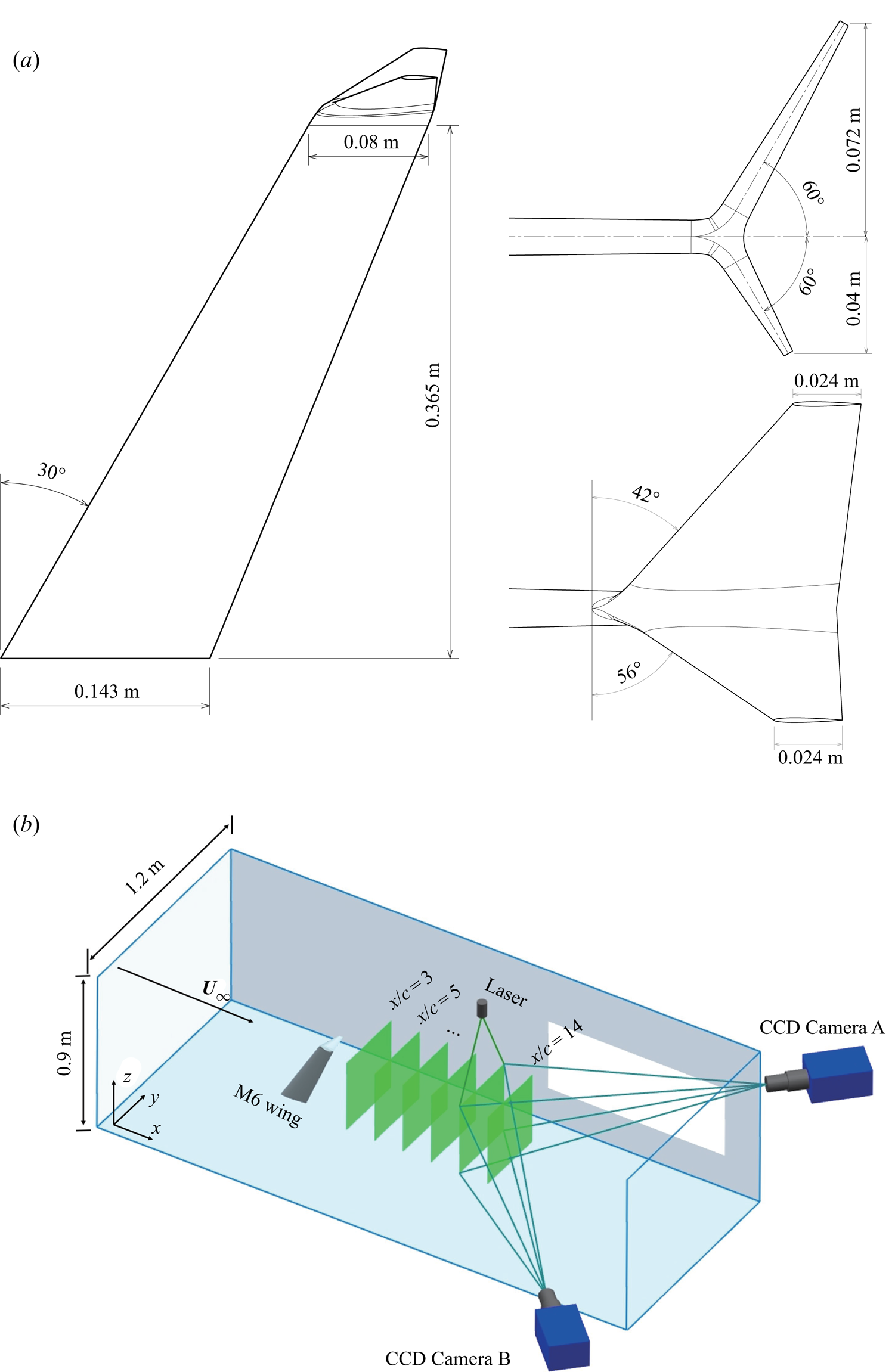
 $45\ \textrm {m}\ \textrm {s}^{-1}$, and the turbulent intensity was below 0.5 %. The boundary layer thickness was estimated to be less than 3.6 % of the height of the test section. The isolated trailing vortex and the vortex pair were generated by a swept wing of NACA0015 profile without and with a split winglet. The wing adopted the standard M6 wing platform and the winglet was of the Whitcomb configuration (Whitcomb Reference Whitcomb1976). The geometry of the wing platform and the winglet is shown in figure 1(a). The combination of an M6 wing platform and a Whitcomb winglet served to capture the complexity of an aircraft wingtip while remaining a clean, canonical wing model. The wing root was attached to an endplate to avoid any influence from the wind-tunnel boundary layer, as in Birch et al. (Reference Birch, Lee, Mokhtarian and Kafyeke2004). The wing model was mounted on a rail to allow an adjustment of the streamwise locations. The wingtip chord was
 $c = 0.08\ \textrm {m}$, which gave a chord-based Reynolds number of
 $Re_c={U_\infty }c/\nu =0.8\times 10^{5}, 1.6\times 10^{5}$ and
 $2.4\times 10^{5}$ for the three measured free-stream velocities. The incident angle was tuned to
 $6^{\circ }$,
 $8^{\circ }$ and
 $10^{\circ }$ to generate sufficient swirl. A schematic diagram of the SPIV experimental set-up is shown in figure 1(b).
Schematic illustration of (a) the M6 wing model and the winglet geometry, (b) the SPIV set-up.

2.1.2. Velocity measurement
The three-component velocity field at each slice perpendicular to the free stream from  $x/c=3\sim 14$ was measured by a SPIV system. The flow was seeded by droplets of atomized glycol with a diameter of 1 to
 $5\ {\mathrm {\mu }}\textrm {m}$, which were allowed to recirculate in the tunnel until a uniform distribution was achieved. The particles were then illuminated by a double-pulsed Nd:YAG laser (
 $2\times 380$ mJ) of 532 nm wavelength. The beam was formed into a 2 mm-thick light sheet throughout the measured frame using a cylindrical lens. The images were captured by two 12-bit CCD cameras (PCO 2000,
 $2048\times 2048$ pixels) positioned on each side of the test section with a
 $30^{\circ }$ angle of view to the free stream. To capture both vortices in the vortex pair, the calibrated frame of view was adjusted to
 $292\times 269$ mm, which yielded a raw-image resolution of
 $0.13\ \textrm {mm}\ \textrm {pixel}^{-1}$. The cameras and the laser were synchronized by a digital delay generator (DG646), and the time interval between two consecutive shots was tuned to
 ${\Delta }t=15\ {\mathrm {\mu }}\textrm {s}$,
 $7.5\ {\mathrm {\mu }}\textrm {s}$,
 $4\ {\mathrm {\mu }}\textrm {s}$ for
 $U_\infty =15\ \textrm {m}\ \textrm {s}^{-1}$,
 $30\ \textrm {m}\ \textrm {s}^{-1}$,
 $45\ \textrm {m}\ \textrm {s}^{-1}$, respectively, to ensure that the particles in each image pair remained in the light sheet. For each measured flow condition, 300 consecutive images were captured at a sampling frequency of 1 Hz to obtain the time-averaged flow field. The velocity vectors were then acquired using the cross-correlation algorithm built in the TSI Insight 4G software. Double interrogation windows were used to improve the resolution of the velocity vectors, with a starting interrogation window of
 $72\times 72$ pixels and an ending window of
 $36\times 36$ pixels. The unresolved vectors were interpolated by the surrounding vectors with a filling size of
 $9\times 9$ pixels. The resulting percentage of good vectors was over 85 %. The relative uncertainties of the in-plane velocities and the derived streamwise vorticity were 1 % and 3 %, respectively.
2.1.3. Parameters and models of trailing vortex
The trailing vortex is characterized by its core radius  $\delta$, axial velocity deficit
 $\xi$ and circulation
 $\varGamma$. The Reynolds number for the vortex is
 $Re_\delta = \xi \delta /\nu$ as in Mayer & Powell (Reference Mayer and Powell1992) and Fabre & Jacquin (Reference Fabre and Jacquin2004). These parameters were extracted by fitting the measured vortex with the Batchelor vortex, which reads in cylindrical coordinates as
 \begin{equation} U_\theta=\frac{\varGamma}{2 {\rm \pi}r}\left( 1-\exp\left(- \frac{r^{2}}{{\delta}^{2}}\right) \right),\quad U_r=0,\quad U_x=U_\infty-\xi\exp\left(- \frac{r^{2}}{{\delta}^{2}}\right). \end{equation}
The swirl number is thus  $q = \varGamma /(2{\rm \pi} \delta \xi )$, and the axial vorticity can be written as
 \begin{equation} \omega_x=\frac{\varGamma}{{\rm \pi}\delta^{2}}\exp\left( - \frac{r^{2}}{{\delta}^{2}} \right). \end{equation}
2.2. Stability analysis and numerical methods
2.2.1. Governing equations
Considering the range of free-stream velocities measured in the present study, the incompressible, linearized Navier–Stokes equations (LNSEs) were used in the stability analysis. For the isolated trailing vortex, owing to its axial symmetry, the governing equations were transformed onto non-dimensionalized cylindrical coordinates  $(\tilde {r},\theta ,\tilde {x})$. The equations were non-dimensionalized by the chord length and the free-stream velocity. These parameters corresponded to a core-radius-based Reynolds number of
 $Re_c\tilde {\delta }=14\,000$ to
 $58\,000$. The instantaneous flow field
 $\boldsymbol {q}=[u_r,u_\theta ,u_x,p]^{\textrm {T}}$ was decomposed into a steady basic state
 $\bar {\boldsymbol {q}}$ and an infinitesimal perturbation term
 $\boldsymbol {q}'$. The perturbation
 $\boldsymbol {q}'$ was then spanned into a Fourier series in the axial, tangential and timewise directions where the flow can be considered homogeneous, written as
 \begin{equation} {\boldsymbol{q'}}(\tilde{r},\theta,\tilde{x},\tilde{t})={\hat{\boldsymbol{q}}}(\tilde{r})\exp[\textrm{i}\left( {\alpha}\tilde{x}+m\theta-{\omega}\tilde{t} \right))]+\boldsymbol{c.c.} \end{equation}
in which  $\alpha$ is the axial wavenumber,
 $m$ is the azimuthal wavenumber,
 $\omega$ is the frequency, c.c. is the conjugate complex and
 ${\hat {\boldsymbol {q}}}=[\textrm {i} \hat {u}_r,\hat {u}_\theta ,\hat {u}_x,\hat {p}]^{\textrm {T}}$ is the eigenvector. Here, the temporal local analysis is performed by solving the generalized eigenvalue problem (EVP)
 $\boldsymbol{\mathsf{A}}\hat {\boldsymbol{q}}={\omega }{\boldsymbol{\mathsf{B}}\hat {\boldsymbol{q}}}$ rearranged from the LNSE, where
 $\omega =\omega _r+\textrm {i}\omega _i$ is the complex frequency. The real part
 $\omega _r$ is the frequency of the perturbation and the imaginary part
 $\omega _i$ corresponds to the growth rate.
Differing from the isolated trailing vortex, while the parallel assumption still holds in the streamwise direction for a fully-developed vortex pair, the axial symmetry is broken for the vortex pair. Therefore, bi-global linear stability analysis was performed in the vortex pair scenario, which was conducted in non-dimensionalized Cartesian coordinates  $(\tilde {x}, \tilde {y}, \tilde {z})$ with
 ${\boldsymbol {q}}=[u,v,w,p]^{\textrm {T}}$. All parameters and governing equations were non-dimensionalized by the core radius
 $\delta$ and characteristic velocity
 $U_c=\varGamma /2{\rm \pi} \delta$ of the upper vortex in the vortex pair. The bi-global analysis then allowed for resolved gradients in the cross-wise directions
 $(\tilde {y}, \tilde {z})$, and treated the streamwise gradient as the span of the Fourier series. The infinitesimal perturbation in the bi-global framework is hence given by
 \begin{equation} \boldsymbol{q'}(\tilde{x},\tilde{y},\tilde{z},\tilde{t})={\hat{\boldsymbol{q}}}(\tilde{y}, \tilde{z})\exp[\textrm{i}\left( {\alpha}\tilde{x}-{\omega}\tilde{t}\right))]+\boldsymbol{c.c.}\end{equation}
By substituting  $\boldsymbol {q'}$ into the LNSE and transforming the equations into a generalized EVP
 $\boldsymbol{\mathsf{A}}_{\boldsymbol{g}}\hat {\boldsymbol {q}}=\omega \boldsymbol{\mathsf{B}}_{\boldsymbol {g}}\hat {\boldsymbol{q}}$, the complex frequency
 $\omega$ and the associated eigenmode
 ${\hat {\boldsymbol {q}}}=[ \hat {u},\hat {v},\hat {w},\hat {p}]^{\textrm {T}}$ were sorted to quantify the asymptotic instability of the flow. More details of the local and global stability matrices and their boundary conditions are presented in Appendices A1 and A2.
2.2.2. Description of the numerical method
In this work, the Chebyshev spectral collocation method was chosen for discretization in both the local and bi-global linear stability analyses. As the physical domain ranged from  $\tilde {r}=0$ to the truncation length
 $\tilde {r}_{max}$ for the isolated trailing vortex and
 $(\tilde {y}_{min}, \tilde {z}_{min})$ to
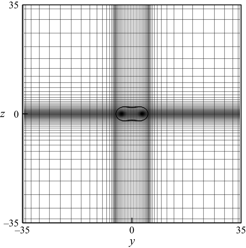
 $(\tilde {y}_{max}, \tilde {z}_{max})$ for the vortex pair, different mapping functions were employed in the local and global analyses to map the Chebyshev collocation points to the physical domain of the problem. A fine-tuned two-dimensional mapping was constructed to resolve both vortices in the vortex pair scenario, whose details can be found in Appendix A3.
The discretized EVP was then solved by the QR method for the local analysis. For the bi-global analysis, the QR method was only used when a full eigenvalue spectrum was needed. The spurious eigenvalues were filtered by their dependence upon discretization according to Oberleithner et al. (Reference Oberleithner, Sieber, Nayeri and Paschereit2011). To save computational cost, the global eigenmodes were acquired by the Arnoldi algorithm.
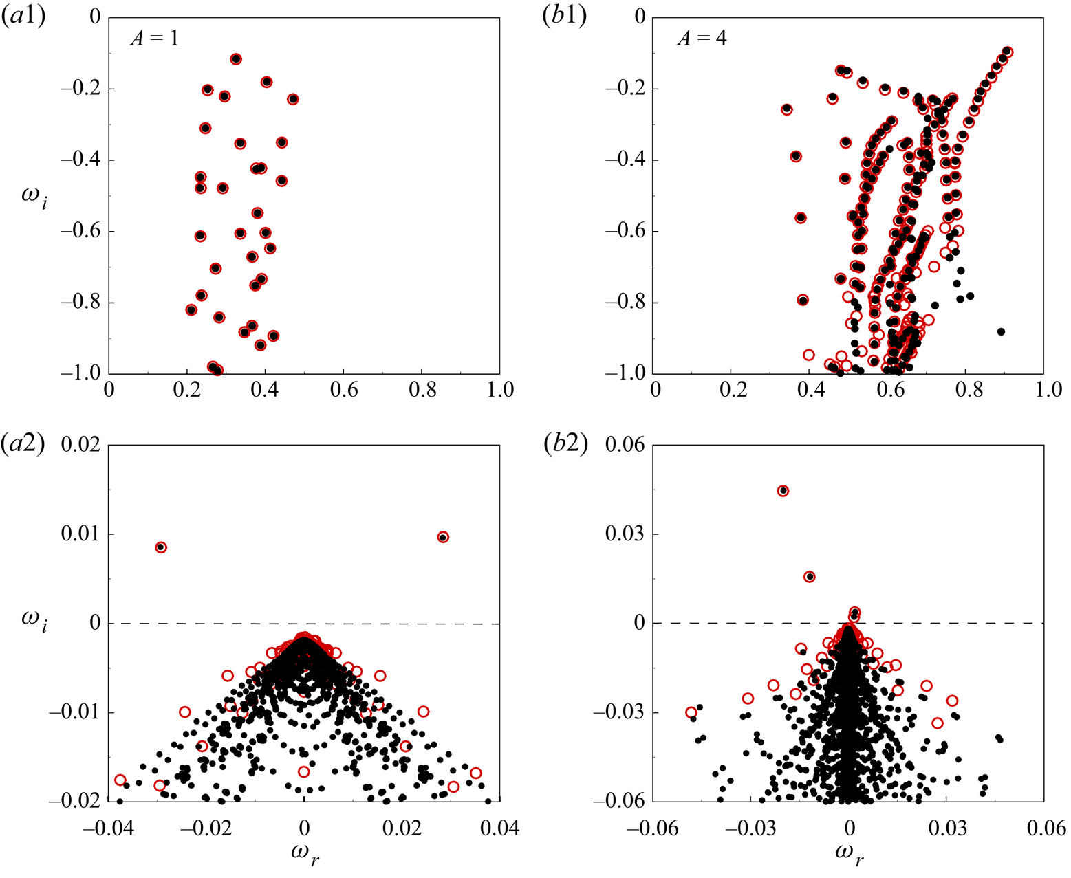
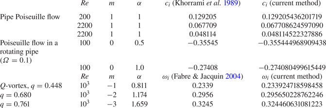
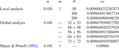
The numerical methods and mapping functions have been validated by Khorrami, Malik & Ash (Reference Khorrami, Malik and Ash1989), Mayer & Powell (Reference Mayer and Powell1992), Theofilis, Duck & Owen (Reference Theofilis, Duck and Owen2004) and Hein & Theofilis (Reference Hein and Theofilis2004). For the local analysis, the temporal growth rates for the classical pipe Poiseuille flow with/without rotation and the  $q$-vortex model were acquired by the present method, which agreed with the published data to at least four significant digits (see table 3 in Appendix B.1). The bi-global stability code was validated by the published data for the duct flow and vortex/vortex pair. The results showed excellent agreement with Theofilis et al. (Reference Theofilis, Duck and Owen2004), Hein & Theofilis (Reference Hein and Theofilis2004) and the local results of Mayer & Powell (Reference Mayer and Powell1992) (see figure 28 in Appendix B.1). A grid-convergence verification (table 4) resulted in a collocation point of
 $N = 200$ for the local analysis and
 $(N_Y, N_Z) = (72, 72)$ for the bi-global analysis.
3. Dynamics of the trailing vortex
3.1. Basic state of the isolated trailing vortex
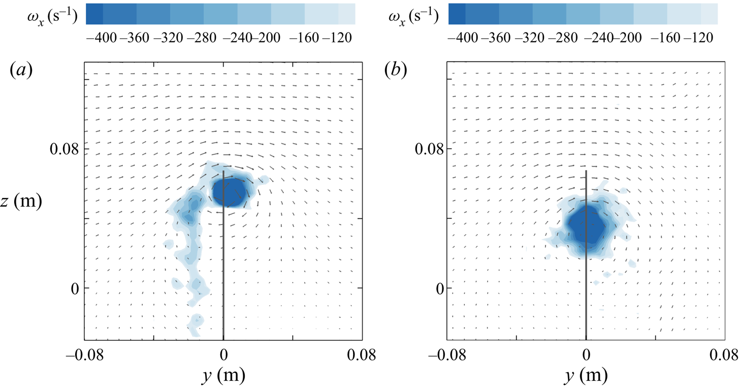
The time-averaged flow field of an isolated trailing vortex is presented in figure 2. In the near-field, the flow field consisted of an isolated vortex at the wingtip and a weak wake generated by the trailing edge of the swept wing, which was being entrained to the vortex. As the vortex propagated further downstream, it translated towards the wing root and evolved into one fully-developed vortex. At this stage, the wake was completely dissipated.
Time-averaged axial vorticity of the isolated trailing vortex: (a)  $x/c = 3$; (b)
 $x/c = 14$. The flow condition is
 $AoA = 6^{\circ }, U_\infty = 30\ \textrm {m}\ \textrm {s}^{-1}$. The solid line sketches the location of the trailing edge. The vector field shows one out of two vectors for clearer illustration.

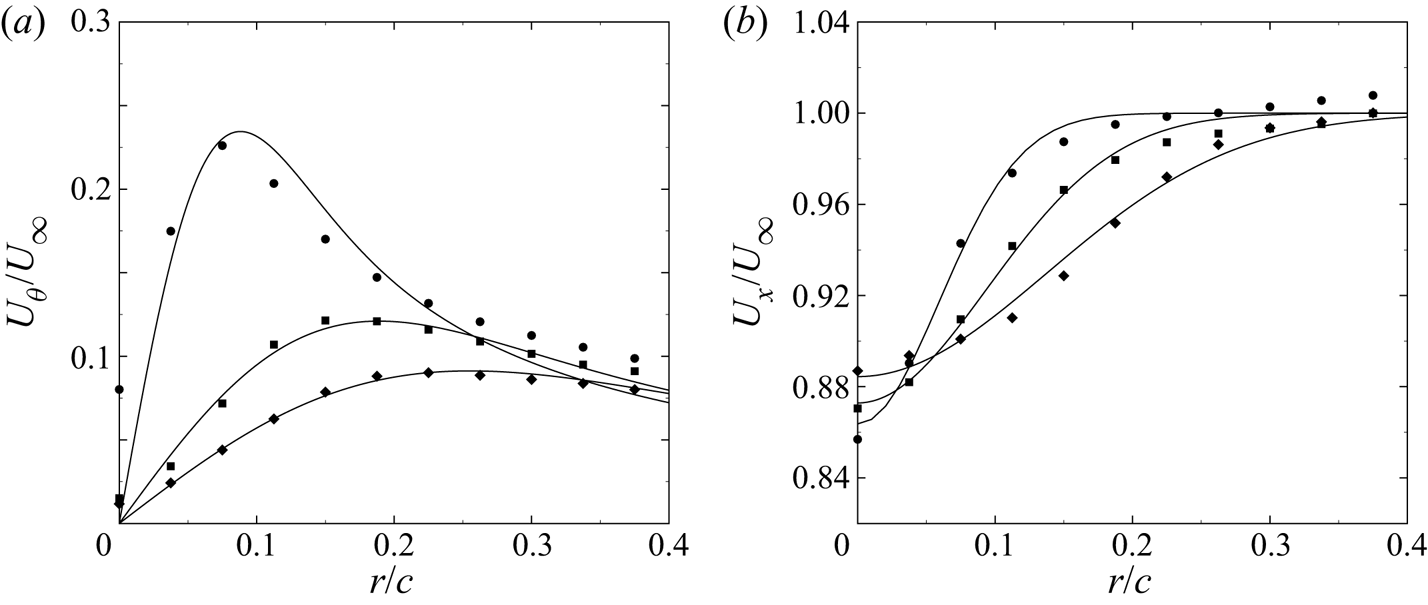
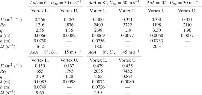
Figure 3 shows the tangential and axial velocity profile of the trailing vortex. The vortex profiles were acquired by azimuthal averaging the flow field about the vortex centre. The vortex centre is identified by the centroid of vorticity as defined in Bertényi & Graham (Reference Bertényi and Graham2007). The azimuthally-averaged profiles were then fitted to the Batchelor vortex in a least-square sense. In figure 3, both velocity profiles were shown to agree well with those of the Batchelor vortex. Owing to a larger bias error in the out-of-plane velocity in the SPIV measurement (Zang & Prasad Reference Zang and Prasad1997), there were some deformations in the axial velocity profile, but the overall profile was correctly captured. The radial velocity was, at most, only a fraction of 0.7 % compared with the free-stream velocity for all measured cases, so was therefore omitted herein. Notably, as the vortex propagated downstream and became fully-developed, the tangential velocity matched better with the Batchelor vortex. The fitted profiles of the non-dimensionalized, fully-developed trailing vortex then served as the base flow in the local analysis presented in § 4. A fast growth of the vortex core is also shown in figure 3 by the shift of the tangential velocity peak. Owing to the effect of diffusion, the tangential velocity and axial velocity deficit decayed rapidly with increasing streamwise distance. The parameters of the measured trailing vortex are tabulated in table 1 for each flow condition.
Streamwise evolution of the isolated trailing vortex: (a) azimuthal velocity and (b) axial velocity. The symbols represent the azimuthally-averaged profile by SPIV,  ${\bigcirc}$,
 $x/c = 5$;
 $\blacksquare$,
 $x/c = 10$;
 $\blacklozenge$,
 $x/c = 14$. The solid curve denotes the fitted profile. The flow condition is
 $AoA = 6^{\circ }, U_\infty = 30\ \textrm {m}\ \textrm {s}^{-1}$.

Parameters of the isolated trailing vortex measured in the experiment.

3.2. Basic state of the co-rotating vortex pair
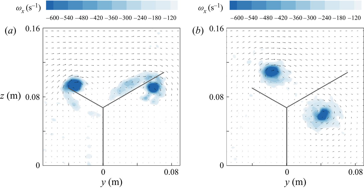
The Whitcomb winglet mounted on the M6 wing generates an approximately equal-strength co-rotating vortex pair. In the present study, the trailing vortex generated by the upper section of the winglet is denoted as the ‘upper vortex’ and, accordingly, ‘lower vortex’ by the lower section. Figure 4 shows the streamwise evolution of the upper and lower vortex. Owing to mutual induction, the two vortices rotated about each other in the same direction as the self-rotation. Their vortex parameters are tabulated in table 2. For all measured cases,  $\delta /b$ was less than the threshold of merger (
 $\delta /b=0.23$ as in Roy et al. Reference Roy, Schaeffer, Le Dizés and Thompson2008), which indicated that no merger had occurred. The circulation of each vortex was hence evaluated individually by fitting the Batchelor vortex to the measured profile of each vortex.
Time-averaged axial vorticity distribution of the co-rotating vortex pair at  $AoA = 8^{\circ }, U_\infty = 30\ \textrm {m}\ \textrm {s}^{-1}$: (a)
 $x/c = 3.0$; (b)
 $x/c = 14$. The solid lines sketch the location of the trailing edges. The vector field shows one out of two vectors for clearer illustration.

Parameters of the co-rotating vortex pair. Vortex L. denotes the lower vortex; Vortex U. denotes the upper vortex.

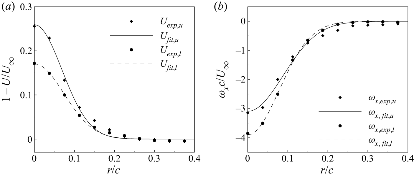
The result of fitting is presented in figure 5. The axial velocity defect and axial vorticity of both the upper and lower vortex agreed well with the Batchelor vortex. Notably, despite an approximately equal circulation (see table 2), the upper vortex had a stronger axial velocity deficit but weaker axial vorticity at the vortex centre compared with the lower vortex. The difference was attributed to the asymmetry of the Whitcomb winglet. Consequently, the upper vortex was of a smaller swirl number. The trend was maintained in each measured flow condition in the present study, as demonstrated in table 2.
Profiles of the co-rotating vortex pair at  $AoA = 8^{\circ }, U_\infty = 30\ \textrm {m}\ \textrm {s}^{-1}$,
 $x/c = 14$: (a) axial velocity defect and (b) azimuthally-averaged axial vorticity. The subscript
 $u$ denotes the upper vortex;
 $l$ denotes the lower vortex. Symbols, SPIV data; curves, fitted vortex profile.

3.3. Vortex wandering phenomenon
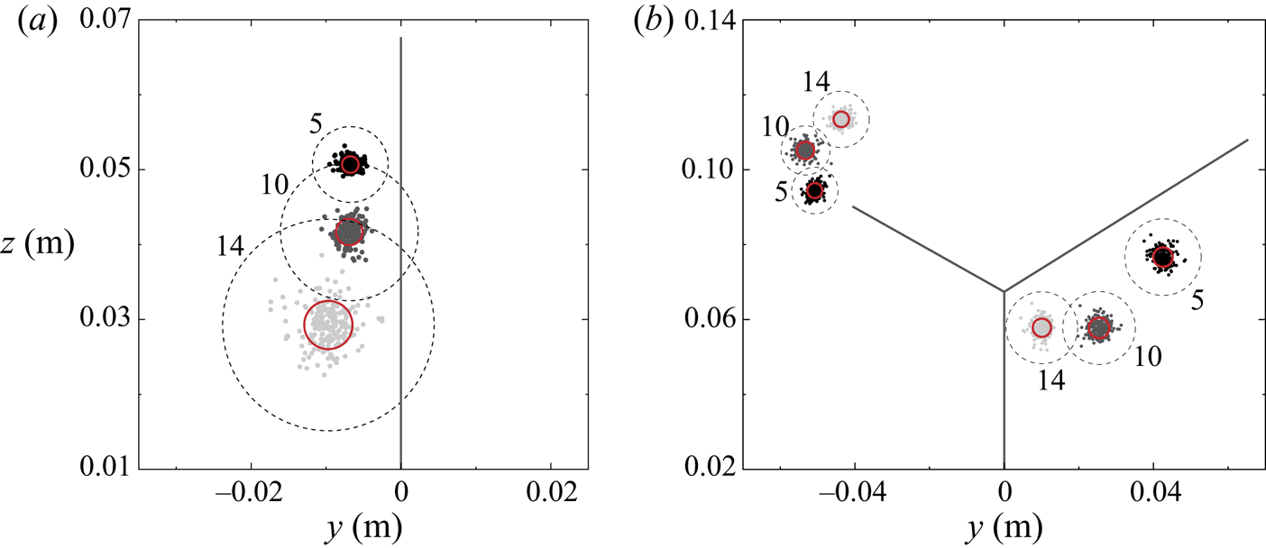
An intuitive manifestation of the trailing vortex instability is the vortex wandering phenomenon (Roy et al. Reference Roy, Leweke, Thompson and Hourigan2011; Cheng et al. Reference Cheng, Qiu, Xiang and Liu2019). The phenomenon was observed for both the isolated trailing vortex and the co-rotating vortex pair, as shown in figure 6. The vortex centres of the isolated vortex quickly became scattered downstream, which resulted in a rapid increase in the wandering amplitude. For the co-rotating vortex, each vortex oscillated about its mean centre while rotating about each other. The wandering amplitudes did not exceed the core size for both configurations.
Phenomenon of vortex wandering for (a) isolated trailing vortex, (b) co-rotating vortex pair. The symbols represent the instantaneous vortex centres. The red solid circle denotes the wandering amplitude obtained as the standard deviation of the vortex centres, as in Bailey & Tavoularis (Reference Bailey and Tavoularis2008), and the dashed circle denotes the vortex core.

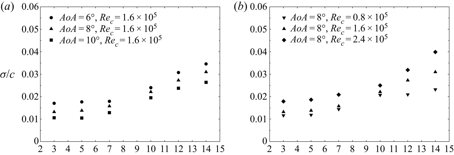
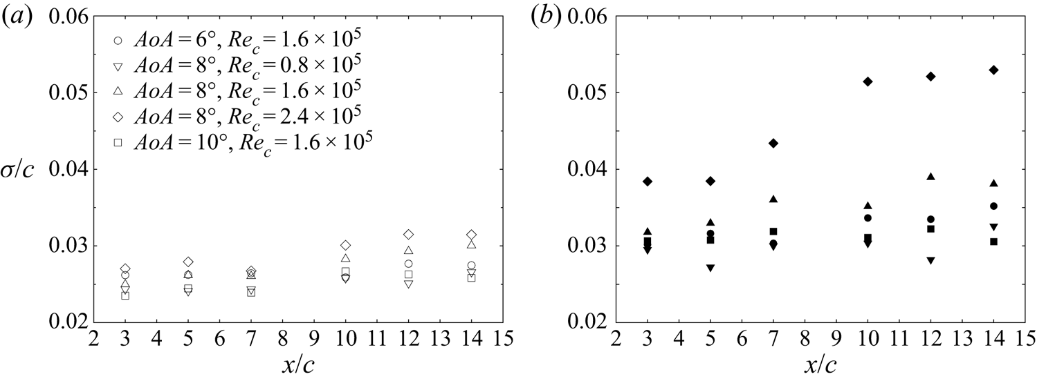
Figure 7 quantitatively shows the wandering amplitude along each measured streamwise position. For both vortex configurations, the wandering amplitude monotonously increased downstream. The same trend has been reported by Bailey & Tavoularis (Reference Bailey and Tavoularis2008) for a single trailing vortex. The wandering amplitude of the isolated trailing vortex was of the same magnitude as the ‘no-grid’ case in Bailey & Tavoularis (Reference Bailey and Tavoularis2008), if both were normalized by the core radius. Notably, for the isolated vortex, the wandering amplitude at a smaller incident angle, which corresponded to a gentler swirl (see table 1), was consistently larger than that of a larger incident angle. The same was true for the vortex pair, where the upper vortex, which was of a gentler swirl, manifested a larger wandering amplitude (figure 8). The observation suggested that the trailing vortex is more stable with a larger swirl. Meanwhile, the normalized wandering amplitude showed a positive correlation with the Reynolds number for both vortex configurations. These findings agree with the results of Mayer & Powell (Reference Mayer and Powell1992) and Fabre & Jacquin (Reference Fabre and Jacquin2004), where the q-vortex was stabilized beyond a critical swirl number and the overall maximum of the growth rate was damped by viscosity.
Streamwise variation of the normalized wandering amplitude for the isolated trailing vortex, (a) with different  $AoA$, (b) with different
 $Re_c$.

Normalized wandering amplitude along the streamwise direction of each vortex in the co-rotating pair: (a) the lower vortex (hollow symbols); (b) the upper vortex (solid symbols).

4. Instability characteristics of the isolated trailing vortex
4.1. Identification of perturbation modes
4.1.1. Spectra and mode shape with different azimuthal wavenumbers
In the scenario of the isolated trailing vortex, local stability analysis was performed on the measured vortex profiles, which were fitted to the Batchelor vortex. The purpose of fitting the measured vortex to a Batchelor vortex is to obtain a base flow as an exact solution of the N–S equation (Theofilis Reference Theofilis2003). The measured velocity profiles were not recentred to correct for vortex wandering before fitting, as the wandering amplitude was sufficiently small in the present research to have negligible effect on the mean profile. Owing to an inversion of the axial direction in the Batchelor vortex used herein, the direction of the azimuthal wavenumber  $m$ here was opposite to that in Lessen et al. (Reference Lessen, Singh and Paillet1974), Lessen & Paillet (Reference Lessen and Paillet1974), Khorrami (Reference Khorrami1991) and Fabre & Jacquin (Reference Fabre and Jacquin2004). In this research, modes with positive
 $m$ represent perturbations countering the vortex rotation, and vice versa for negative
 $m$.
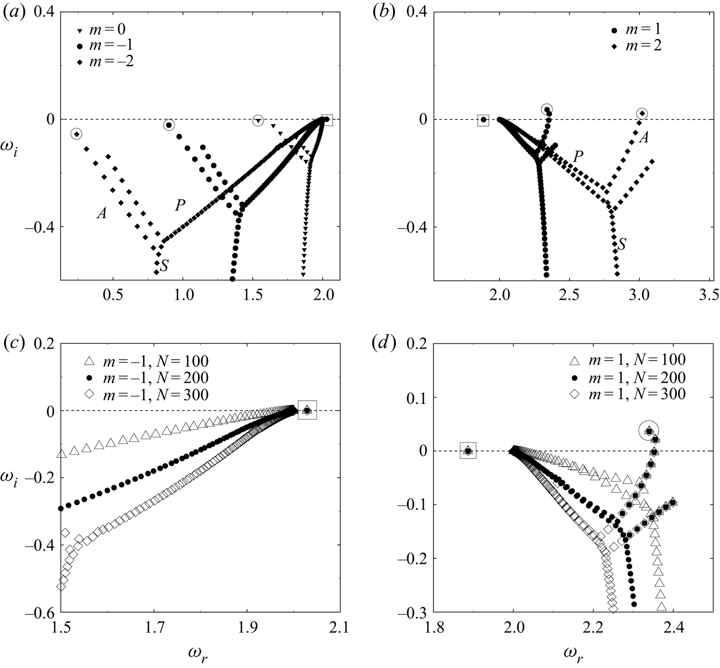
Figure 9 shows the local eigenspectrum of an isolated trailing vortex for different  $m$ at
 $\alpha = 2$. Each spectrum for
 $m = 0, \pm 1, \pm 2$ consisted of three families. These families shared a similar topology as the A, P and S families categorized by Mack (Reference Mack1976) for the boundary layer. Therefore, we kept the naming used in Mack (Reference Mack1976) for the trailing vortex herein. A convergence study shown in figure 9(c,d) reveals two types of discrete modes in the P and A families. These were named as Mode-P and Mode-A. The structure of these discrete modes, which is transformed from one-dimensional eigenfunctions, is presented in figure 10. The S family, which corresponds to the continuous modes in the free-stream (Mao & Sherwin Reference Mao and Sherwin2011), will not be discussed herein.
Eigenspectra with  $m = 0, \pm 1, \pm 2, \alpha = 2.0$, (a) non-negative
 $m$, (b) negative
 $m$, (c,d) zoomed-in view of the
 $|m| = 1$ spectra with different numbers of collocation points. The flow condition is
 $AoA = 8^{\circ }, Re_c = 1.6\times 10^5$. Mode-P and Mode-A are marked by
 $\square$ and
 ${\bigcirc}$, respectively.

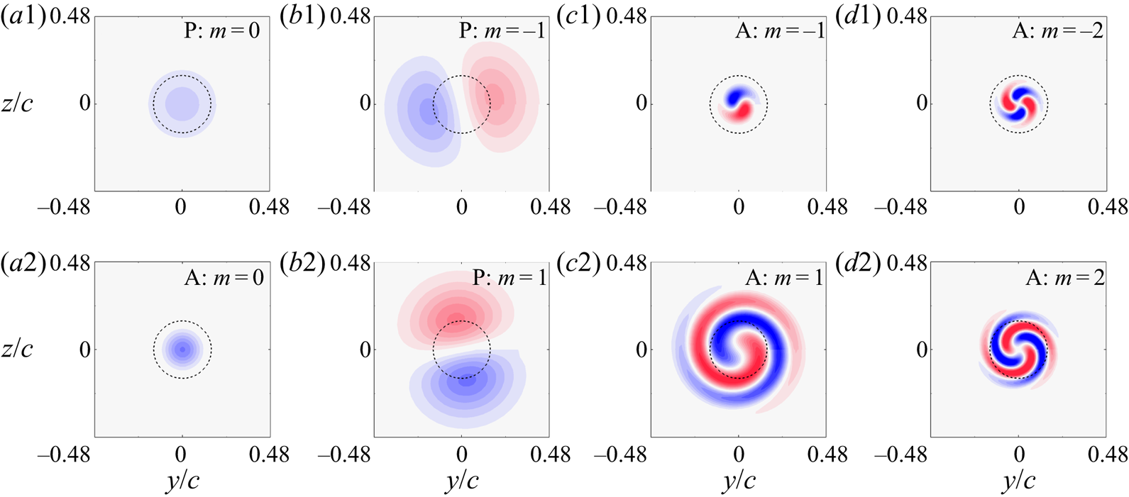
Axial vorticity distribution of Mode-P and Mode-A with  $m = 0, \pm 1, \pm 2$ for
 $\alpha = 2.0$ as marked in figure 9. The contour range is uniformly
 $[-10, 10]$. The dashed circle denotes the vortex core.

From figure 9(a,b), it can be observed that Mode-P was exclusive for  $|m|\leqslant 1$, and was otherwise missing for higher
 $|m|$. Such a mode was neutral given its closeness to
 $\omega _i=0$. Mode-P with
 $m = 0$ is an axisymmetric mode (figure 10a1); and Mode-P with
 $|m| = 1$ is of a dipole structure, which corresponds to a displacement wave (figure 10b1,b2). The latter gives rise to the coherent motion of vortex wandering (Edstrand et al. Reference Edstrand, Davis, Schmid, Taira and Cattafesta2016).
For Mode-A, those with non-positive  $m$ (
 $m = 0, -1, -2$) completely fell into the stable half-plane of the eigenspectrum (figure 9a). Mode-A with
 $m = 0$ was of an axisymmetric structure (figure 10a2), while those with
 $m = -1, -2$ featured a short spiral structure (figure 10c1,d1). For Mode-A with positive
 $m$ (
 $m = 1, 2$), we observed a piercing into the unstable half-plane, which indicated that the measured trailing vortex was temporally unstable with these azimuthal wavenumbers. The observation hence distinguished the measured trailing vortex from the two-dimensional Lamb—Oseen vortex where all the modes were essentially damped (Fabre et al. Reference Fabre, Sipp and Jacquin2006). The structure of Mode-A with positive-
 $m$ featured distinct spiral structures winding around the vortex centre (figure 10c2,d2). This structure was similar to that of the purely viscous mode, as reported by Fabre et al. (Reference Fabre, Sipp and Jacquin2006), but extended further beyond the core radius.
4.1.2. Stability curves for different modes
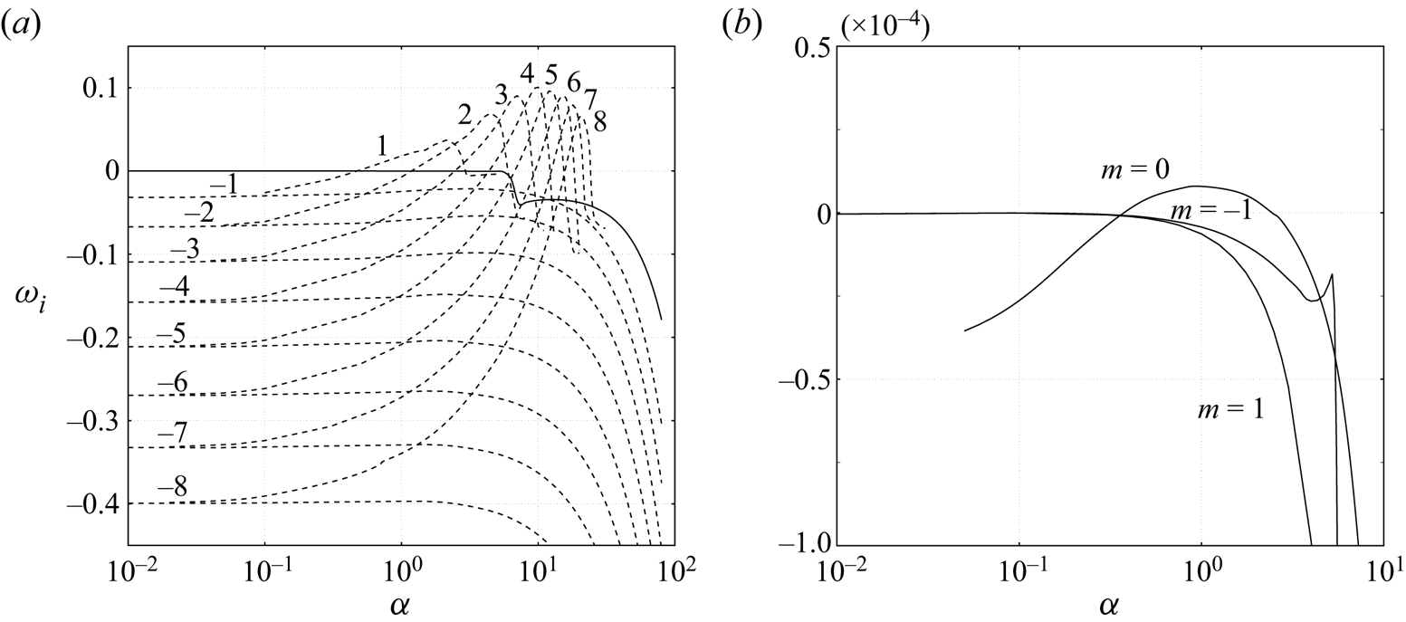
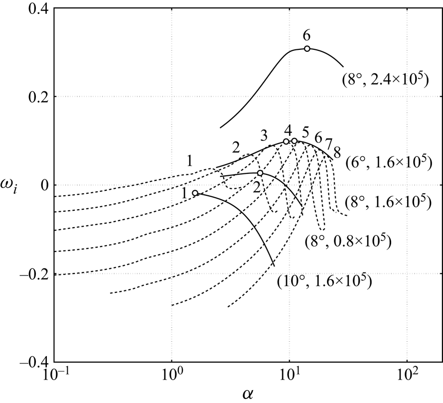
To further quantify the instability of trailing vortex, the growth rates of Mode-P and Mode-A are presented in figure 11 as a function of axial wavenumber  $\alpha$. The resulting curve is referred to as the stability curve in the present study. Figure 11 confirms that the trailing vortex was dominated by Mode-A with positive-m, whose growth rate was the highest amongst all the modes and increased with
 $m$ until
 $m = 4$. Such a mode grew in the asymptotic limit and overwhelmed the other modes. Mode-A with negative-
 $m$ was stabilized monotonously with the increase of
 $|m|$ and remained stable for the entire dispersion relation. Mode-P with
 $|m| \leqslant 1$ remained marginally stable until
 $\alpha = 5.0$, beyond which it was completely stabilized. A zoom-in image of the neutrally stable Mode-P revealed that the
 $m = 1$ mode decayed faster at large axial wavenumbers than the
 $m = -1$ mode and the axisymmetric mode (
 $m = 0$) was indeed marginally unstable.
Growth rate  $\omega _i$ as a function of the axial wavenumber
 $\alpha$ for (a) Mode-P with
 $m = -1$ and Mode-A with
 $m = [-8, 8]$, (b) Mode-P with
 $m = 0, \pm 1$ (zoomed-in view). Solid curves, Mode-P; dashed curves, Mode-A. The labels denote
 $m$ for each curve. The flow condition is the same as that in figure 9.

The characteristics of this dominating Mode-A with positive-m was examined for the rest of the flow conditions. Figure 12 shows that the trailing vortex at  $AoA = 8^{\circ }, Re_c = 2.4\times 10^5$ was the most unstable amongst the measured flow conditions. The corresponding growth rate peaked at
 $m=6$. The envelopes of the stability curves for the trailing vortex at
 $AoA = 6^{\circ }$ and
 $8^{\circ }, Re_c = 1.6\times 10^5$ almost coincided with each other. Both of them peaked at
 $m = 4$ and manifested an unstable nature. For the trailing vortex at
 $AoA = 10^{\circ }$, Mode-A was stabilized, probably owing to an increased swirl, and fell in the stable half-plane.
Envelopes of the Mode-A stability curve at different flow conditions, as shown by the solid lines. The envelope at  $AoA = 8^{\circ }, Re_c = 1.6\times 10^{5}$ is substituted by its stability curves (dashed line) as shown in figure 11 for a better illustration. The labelled brackets denote
 $[AoA, Re_c]$, and the most unstable
 $m$ of each flow condition is marked by
 $\circ$.

It is noticeable from figure 12 that the degree of instability, as demonstrated by the maximum growth rate, matched qualitatively with the wandering amplitude in figure 7. The vortex with a high growth rate, e.g. at  $AoA = 8^{\circ }, Re_c = 1.6\times 10^{5}$ with
 $\omega _{i,max}$ reaching up to 0.3, manifested a larger wandering amplitude than the less unstable vortices, e.g. at
 $AoA = 10^{\circ }, Re_c = 1.6\times 10^{5}$. Such a correlation between the wandering amplitude and the growth rate was also observed for the other flow conditions. In addition, the temporal frequencies of Mode-P (
 $m=-1$) were in the range of 5–15 Hz for the measured condition, which agreed well with the frequencies of vortex wandering reported by Devenport et al. (Reference Devenport, Rife, Liapis and Follin1996) and Bailey & Tavoularis (Reference Bailey and Tavoularis2008) at similar flow conditions.
4.2. Modal structure of perturbations with asymptotic growth
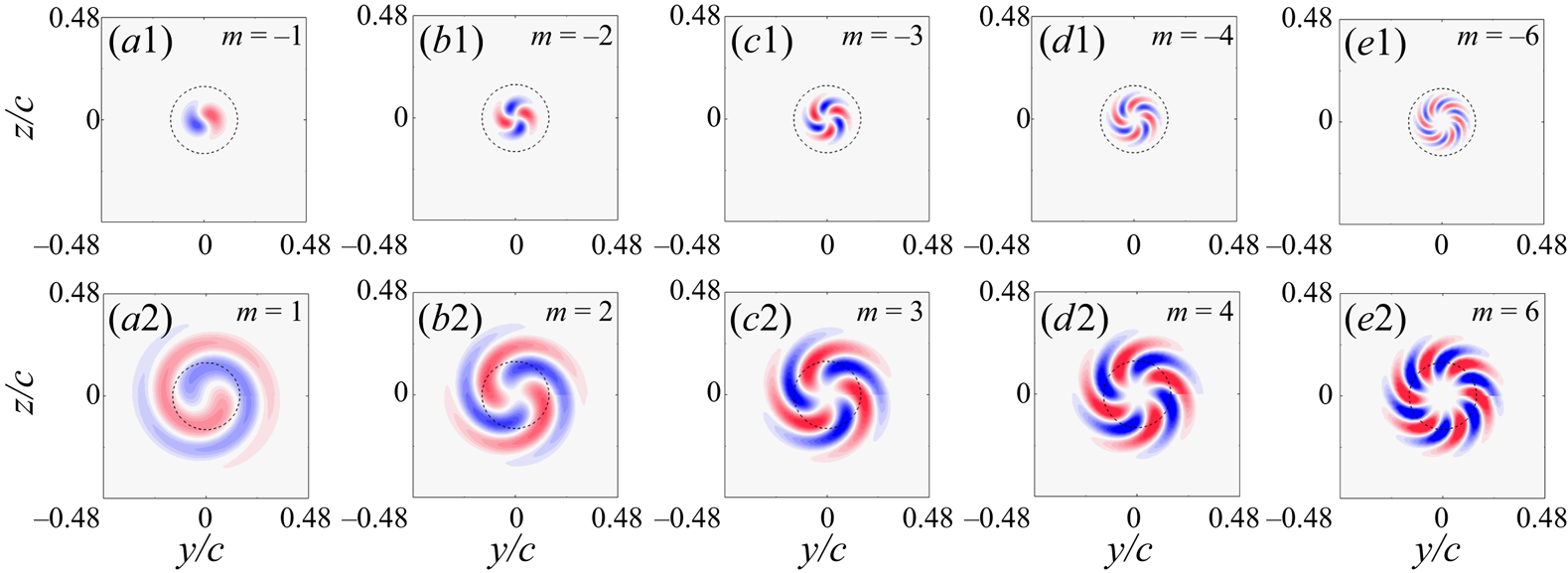
The modal structure of perturbations with asymptotic growth in the isolated trailing vortex is highlighted in figure 13 by comparing the modal structure of Mode-A with positive and negative  $m$. Each mode was featured by a spiral structure stemming from the vortex centre, with the number of its arms readily prescribed by
 $m$. Notably, the perturbed region of dominating Mode-A with positive-
 $m$ extended further outside the vortex core. The perturbed region of Mode-A with positive=
 $m$ was significantly larger than that of the stabilized Mode-A with negative-
 $m$. The same was observed throughout the
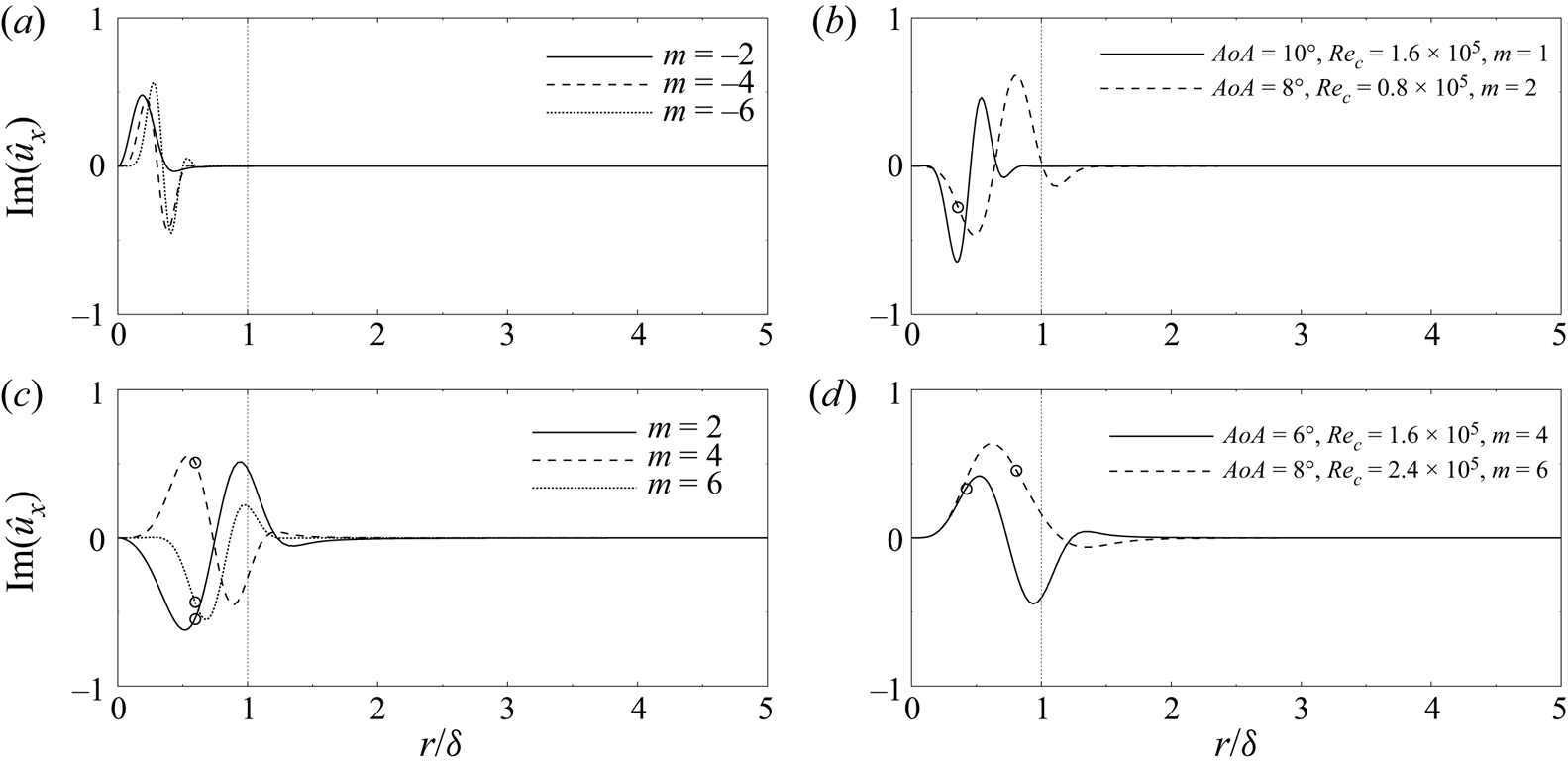
 $m$-branch of the dispersion relation. A further illustration in terms of the profiles of
 $\hat {u}_x$ is shown in figure 14. The perturbation of Mode-A with negative-
 $m$ was confined compactly near the vortex centre, while those with positive-m uniformly spread across the core boundary (figure 14a,c). The distinct difference in these perturbation modes suggested a potential correlation underlying asymptotic growth and the radial extent of perturbations with regards to the core region, which holds across different flow conditions. For instance, in figure 14(b,d), the damped mode at
 $AoA = 10^{\circ }, Re_c = 1.6\times 10^{5}$ and the less unstable mode at
 $AoA = 8^{\circ }, Re_c = 0.8\times 10^{5}$ were more clustered towards the vortex centre, while the modes with higher growth rates (
 $AoA = 6^{\circ }, Re_c = 1.6\times 10^{5}$;
 $AoA = 8^{\circ }, Re_c = 2.4\times 10^{5}$) extended further beyond the vortex core.
Structure of Mode-A with different azimuthal wavenumbers at  $AoA = 8^{\circ }, Re_c = 1.6\times 10^{5}$, each corresponding to the most amplified mode at the peak of the stability curves in figure 11. The axial vorticity contour range is
 $[-20, 20]$ for each subplot.

Eigenfunctions of the axial velocity perturbation  $\hat {u}_x$, (a,c) Mode-A with different
 $m$ at
 $AoA = 8^{\circ }, Re_c = 1.6\times 10^{5}$, (b,d) the most amplified Mode-A at different flow conditions. The circles mark the critical radius predicted by using Leibovich & Stewartson's theory (Reference Leibovich and Stewartson1983).

According to Leibovich & Stewartson (Reference Leibovich and Stewartson1983), the perturbation modes of a columnar vortex are centred at a critical radius where they obtain the maximum growth rate. The critical radii corresponding to the measured trailing vortex are marked on the eigenfunctions in figure 14. A general agreement was observed where the critical radius located where the perturbation was clustered. The slight error was attributed to the inviscid nature of Leibovich & Stewartson's analysis (Reference Leibovich and Stewartson1983). Notably, the critical radius did not exist at  $AoA = 10^{\circ }, Re_c = 1.6\times 10^{5}$, as the predicted growth rate vanished in this case owing to the damped nature of this mode. The critical radius where the perturbation was most amplified agreed well with Leibovich & Stewartson's theory (Reference Leibovich and Stewartson1983). However, it is still unclear why modes with particular
 $m$ overwhelm other modes and gain the maximum growth rate, e.g. the positive-
 $m$ modes versus the negative-
 $m$ modes. Results here indicate that the permeation of the discrete modes through the core boundary may affect vortex instability. This subject will be further investigated in § 6.
5. Instability characteristics of the co-rotating vortex pair
5.1. Global spectra and perturbation modes
Because the axial symmetry of the base flow was broken in the vortex-pair scenario, bi-global stability analysis was adopted to acquire the instability feature. In the present study, the bi-global analysis was performed upon the time-averaged co-rotating vortex pair at the fixed streamwise position of  $x/c=14$, with the frame of reference fixed to the ground. At the ground frame of reference, the spiral trajectory of the vortices was invariant with time, hence a steady base flow
 $\bar {\boldsymbol {u}}$ existed at any fixed streamwise position. For the measured vortex pair, the streamwise gradient was sufficiently small by a factor of less than 0.03 compared with the transverse gradient in
 $\tilde {y}$ and
 $\tilde {z}$. The flow was therefore considered locally parallel so that the Fourier span in
 $\tilde {x}$, as explicitly given in (2.4), was justified. Meanwhile, owing to the confinement of the frame of view in the SPIV set-up and experimental noise, the experimental measurement is often not directly applicable in global stability analyses (Theofilis Reference Theofilis2003). A processing routine, with reference to Le Dizès & Verga (Reference Le Dizès and Verga2002) and Roy et al. (Reference Roy, Schaeffer, Le Dizés and Thompson2008, Reference Roy, Leweke, Thompson and Hourigan2011), was therefore applied to smooth the raw SPIV data. The measured velocity profiles of the upper and lower vortices were first extracted as the Batchelor vortex and were then allowed to relax to an equilibrium state by evolving in the two-dimensional N–S equation. The equilibrium state was achieved after a short period of oscillation in total circulation. This smoothed field of the time-averaged vortex pair was then taken as the base flow in the global stability analysis, with the axial velocity imposed by its analogy to the axial vorticity distribution as in Roy et al. (Reference Roy, Schaeffer, Le Dizés and Thompson2008, Reference Roy, Leweke, Thompson and Hourigan2011). Detailed reviews of the global analysis applied in vortex systems can be found in Theofilis (Reference Theofilis2003, Reference Theofilis2011).
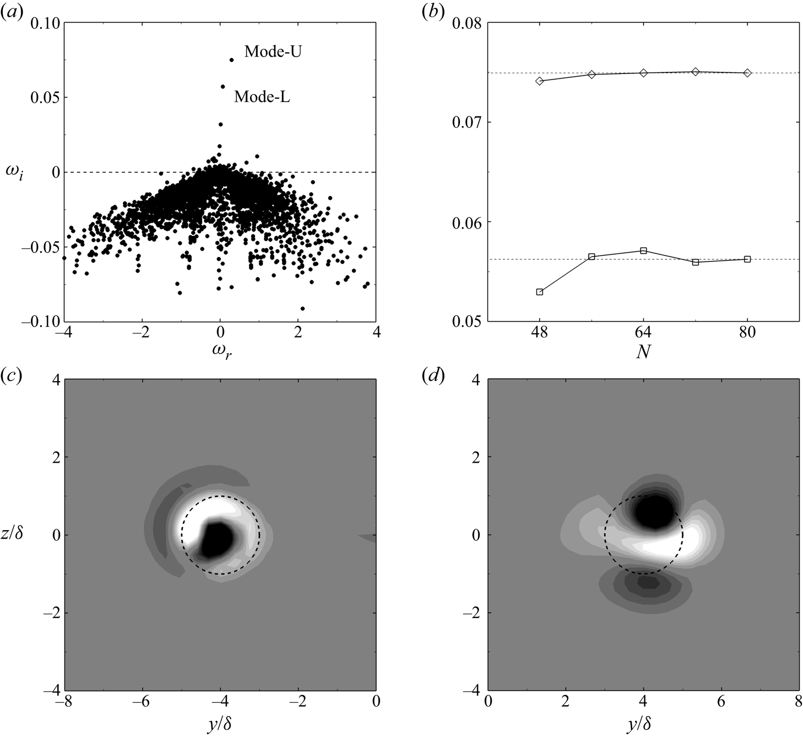
The global spectrum of the co-rotating vortex pair is presented in figure 15. The spectrum consisted of a branch of discrete modes permeating into the unstable half-plane and a conic continuous branch locating in the stable half-plane. The spurious eigenvalues caused by the finite discretization of the physical domain were filtered by their dependence on the grid resolution (Oberleithner et al. Reference Oberleithner, Sieber, Nayeri and Paschereit2011), with a maximum tolerance of 0.01. The convergence study of the growth rate of the two most-amplified discrete modes yielded an acceptable grid resolution of  $72^{2}$ Chebyshev points (figure 15b). The two most-amplified modes were spatially located at the core of the lower vortex (figure 15c) and upper vortex (figure 15d). We therefore denote them as Mode-L for the lower vortex and Mode-U for the upper vortex. Notably, Mode-L and Mode-U resembled the theoretically predicted modes for co-rotating vortex pairs as reported in Eloy & Le Dizès (Reference Eloy and Le Dizès1999) and Lacaze et al. (Reference Lacaze, Ryan and Le Dizès2007), namely the
 $(-1, 1)$ mode and the
 $(-2, 0)$ mode. It was also observed that Mode-U was more unstable than Mode-L owing to its higher growth rate at the given wavenumber.
Global stability results of the co-rotating vortex pair at  $AoA = 8^{\circ }$,
 $Re_c = 1.6\times 10^{5}$,
 $\alpha = 1.25$. (a) Spectrum; (b) convergence study:
 $\lozenge$ Mode-U,
 $\square$ Mode-L; (c,d) the streamwise vorticity distribution for Mode-L and Mode-U, respectively.

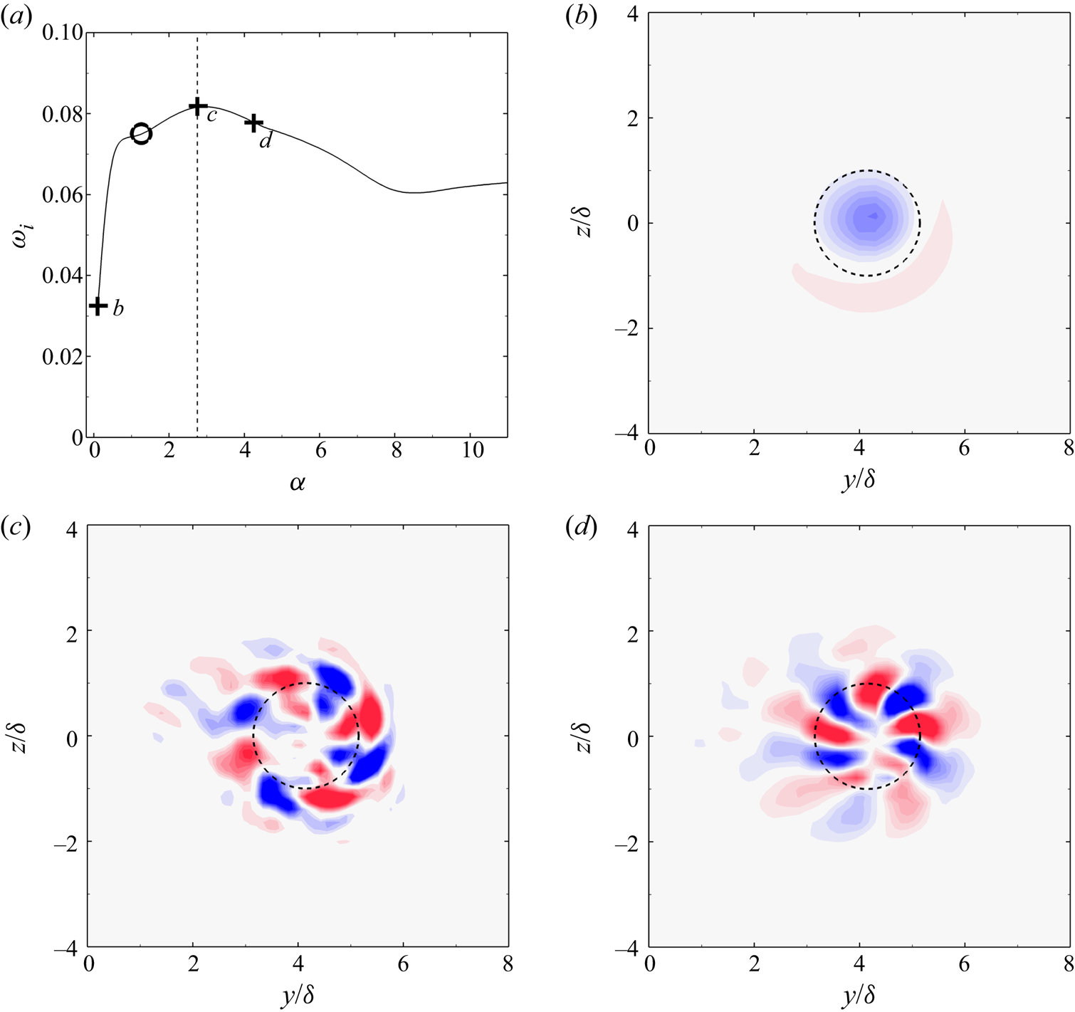
The stability curve and the associated vorticity distribution of Mode-U at  $AoA = 6^{\circ }, Re_c = 1.6\times 10^{5}$ are plotted in figure 16. The variation of its growth rate and modal structure with the axial wavenumber is illustrated. At
 $\alpha = 0.1$, the perturbation mode was of a quasi-axisymmetric structure confined near the vortex centre. With increasing
 $\alpha$, the perturbation featured a larger azimuthal wavenumber and extended beyond the scope of the core region. Notably, the most unstable perturbation was indeed not the canonical
 $(-2, 0)$ mode at
 $\alpha = 1.25$, as shown in figure 15. Instead, the peak of the stability curve corresponded to a dominating mode with larger azimuthal wavenumber, featured by spiral arms surrounding the vortex centre. According to Lacaze et al. (Reference Lacaze, Ryan and Le Dizès2007), this mode was interpreted as the combination of two Kelvin modes with the azimuthal wavenumber of
 $(m_1, m_2) = (-4, -2)$. The axial wavenumber of the
 $(-4, -2)$ mode corresponded to a dominating wavelength of 0.02 m. This was orders of magnitude smaller than the wavelength of mutual induction of the vortex pair, which was approximately 10 m. The rather small time scale of instability compared with the time scale of mutual induction justified that the base flow could be considered as ‘frozen’ at the measured streamwise location and the flow was locally parallel. As
 $\alpha$ was further increased, the azimuthal wavenumber of the perturbation enlarged to
 $(m_1, m_2) = (-5, -3)$ at
 $\alpha = 4.25$, and continued to enlarge with increasing
 $\alpha$, which is not shown herein for brevity.
Variation of Mode-U with axial wavenumbers. The flow condition is the same as that in figure 15. (a) Growth rate  $\omega _i$ as a function of the axial wavenumber
 $\alpha$, black circle denotes
 $\alpha = 1.25$ as in figure 15 and the dashed vertical line marks the curve summit. (b–d) Streamwise vorticity distribution of Mode-U at
 $\alpha = 0.1, 2.75$ and 4.25.

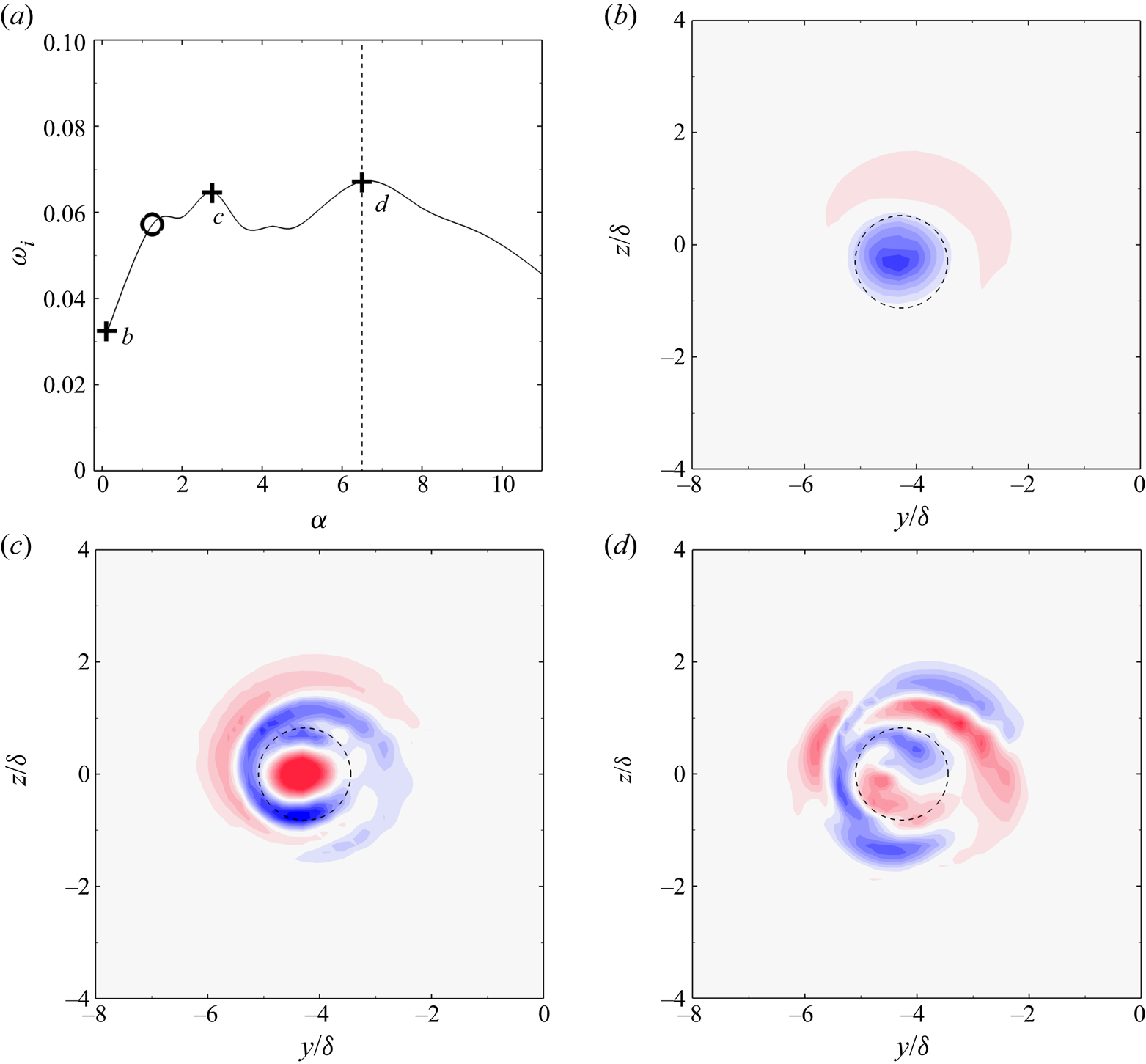
The variation of Mode-L along its stability curve is shown in figure 17. Different from Mode-U, as  $\alpha$ increased, Mode-L featured an increasing radial complexity
 $n$ defined by the zeros along the radial direction, as in Sipp & Jacquin (Reference Sipp and Jacquin2003). At
 $\alpha = 0.1$, the perturbation was of an axisymmetric structure with
 $n = 1$. With increasing
 $\alpha$, the radial complexity increased to
 $n = 2$ and 3 for
 $\alpha = 2.75$ and 6.5, respectively. The most amplified perturbation was observed to be at
 $\alpha = 6.5$ for Mode-L, which featured a radial, wrinkle structure. The difference in the structures of Mode-L and Mode-U was attributed to the different vortex parameters of each vortex. According to table 2, the swirl number of the lower vortex was uniformly over
 $q = 2.5$. Compared with the isolated vortex at
 $AoA = 10^{\circ }$,
 $Re_c = 1.6\times 10^{5}$ (
 $q=1.99$) with damped Mode-A and neutrally-stable Mode-P (see figure 11b), the even stronger swirl of the lower vortex indicated that the vortex should be neutrally stable as an individual vortex. In this parameter range, Mode-P with
 $|m|\leqslant 1$ dominated, which was either dipole shaped or axial symmetric. However, the swirl number of the upper vortex was generally less than 1.5. The swirl number fell into the parameter range where Mode-A with positive-
 $m$ dominates. Therefore, Mode-U resembled Mode-A with positive-
 $m$, which featured an azimuthal structure. It was inferred that the vortex interaction in the co-rotating pair maintained the ‘genre’ of the perturbation mode while revealing the individual features in terms of the radial complexity and azimuthal wavenumber.
Variation of Mode-L with axial wavenumbers. The flow condition is the same as that in figure 15. (a) Growth rate  $\omega _i$ as a function of the axial wavenumber
 $\alpha$. (b–d) Streamwise vorticity distribution at
 $\alpha = 0.1, 2.75$ and 6.5.

5.2. Predominance of the azimuthal mode
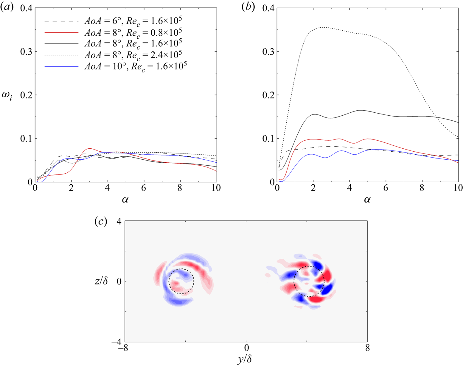
The stability characteristics of the co-rotating vortex pair measured in the experiment were further examined for the rest of the flow conditions. Figure 18 shows that Mode-U was uniformly more unstable than Mode-L, which indicated that the upper vortex was more disturbed than the lower vortex. This instability characteristic was again supported by the results of vortex wandering, where the upper vortex manifested stronger oscillations than the lower vortex (see figures 6 and 8). From the stability curves, the axial wavenumber of both Mode-L and Mode-U was in the range of  $\alpha = [2.75, 5]$. The reference length of
 $\delta \approx 0.01$ m yielded a wavelength of the most unstable perturbation that ranged from 0.01 m to 0.02 m for the measured flow conditions. The wavelength of instability was sufficiently smaller than the wavelength of vortex rotation, owing to mutual induction, and was comparable to the core radius, which suggested that the instability manifested by the measured co-rotating vortex pair was short-wave in nature.
The variation of  $\omega _i$ as a function of
 $\alpha$ for (a) Mode-L and (b) Mode-U at different flow conditions. A representative modal structure for the most unstable Mode-L and Mode-U is shown in (c) at the flow condition of
 $AoA = 6^{\circ }, Re_c = 1.6\times 10^{5}$.

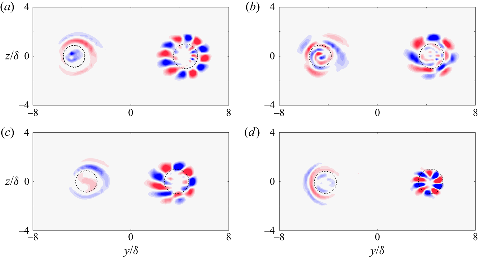
The most unstable modes of the vortex pair for the rest of the flow conditions are demonstrated in figure 19. The two types of perturbation modes prevailed in each co-rotating vortex pair measured in the experiment. For each measured flow condition, Mode-U was of an azimuthal structure with  $m$ varying from 4 to 6, while Mode-L was featured by radial wrinkles. According to the stability curves in figure 18, Mode-U dominated the instability of the vortex pair for all measured flow conditions. It is noteworthy that such predominance of the azimuthal mode also manifested an evident penetration through the core boundary, as was found for the dominating mode in the isolated vortex. From figure 19, it was observed that the azimuthal components of Mode-U permeated the core boundary. The shared feature of the perturbations in both vortex configurations suggested a potential correlation between the modal structure of perturbations and asymptotic growth in trailing vortices.
Streamwise vorticity distribution of the most unstable Mode-L and Mode-U for flow conditions of (a)  $AoA = 8^{\circ }, Re_c = 1.6\times 10^{5}$, (b)
 $AoA = 10^{\circ }, Re_c = 1.6\times 10^{5}$, (c)
 $AoA = 8^{\circ }, Re_c = 1.6\times 10^{5}$, (d)
 $AoA = 6^{\circ }, Re_c = 1.6\times 10^{5}$.

6. A shear-penetration mechanism underlying asymptotic instability
In this section, we seek to shed light on the underlying mechanism for perturbations to undergo asymptotic growth/decay in trailing vortices. The relation of asymptotic perturbations with vortex shear is investigated by introducing a penetration depth for the trailing vortex. The critical points of these perturbations are also given in detail.
6.1. Structure of asymptotic perturbations against vortex shear
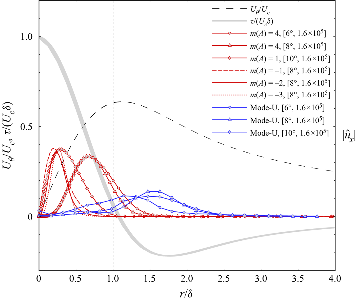
Figure 20 shows that the asymptotic perturbations of trailing vortex were located against the vortex shear. The vortex shear was located at the core boundary, where the non-dimensional azimuthal shear rate  $\tau /(U_c\delta )$ exhibited a steep gradient. A ‘sheltering’ effect also existed for discrete modes stemming from within the vortex core, as it does for the continuous modes reported in Mao & Sherwin (Reference Mao and Sherwin2011). For the isolated vortex, the most-amplified perturbation in each case penetrated the shear layer, e.g. Mode-A of
 $m = 4$ for
 $AoA = 6^{\circ }, 8^{\circ }, Re_c = 1.6\times 10^{5}$, while the other modes with a lower growth rate were confined within, e.g. Mode-A of
 $m = 1$ for
 $AoA = 10^{\circ }, Re_c = 1.6\times 10^{5}$ and the secondary modes for
 $AoA = 8^{\circ }, Re_c = 1.6\times 10^{5}$. Referring to figure 12, all modes that fell in the unstable half-plane managed to overcome the shear-sheltering effect, while the secondary modes were restricted. The same correlation applied to the perturbations of co-rotating vortex pairs. From these observations, one may speculate that the vortex shear confines those less unstable or damped modes in the core and allows asymptotically unstable modes to permeate.
Modal structure of the asymptotic perturbations versus vortex shear. Black dashed line: tangential profile; grey line: shear rate; red line:  $|\widehat {u_x}|$ of the dominating mode in the isolated vortex; red dotted line: secondary mode of the isolated vortex; blue line: the most unstable Mode-U in the co-rotating vortex pair.

6.2. Penetration depth and critical points
In boundary layer flows, the shear-sheltering mechanism can be quantified by a penetration depth defined based on the boundary layer thickness. To quantify the extent of modal perturbations penetrating the vortex shear, the penetration depth  $d$ for trailing vortices is defined based on the core radius as
 \begin{equation} d\equiv\left.\int_{\delta}^{\infty}|\hat{u}_x|\,\textrm{d}r\right/\int_{0}^{\delta}|\hat{u}_x|\,\textrm{d}r. \end{equation}
The penetration depth is thus described as the amount of perturbation outside the core measured by the equivalent amplitude of perturbations inside the core. The amplitude of the axial velocity eigenfunction is employed herein to represent the perturbation.
6.2.1. Shear penetration for the isolated trailing vortex
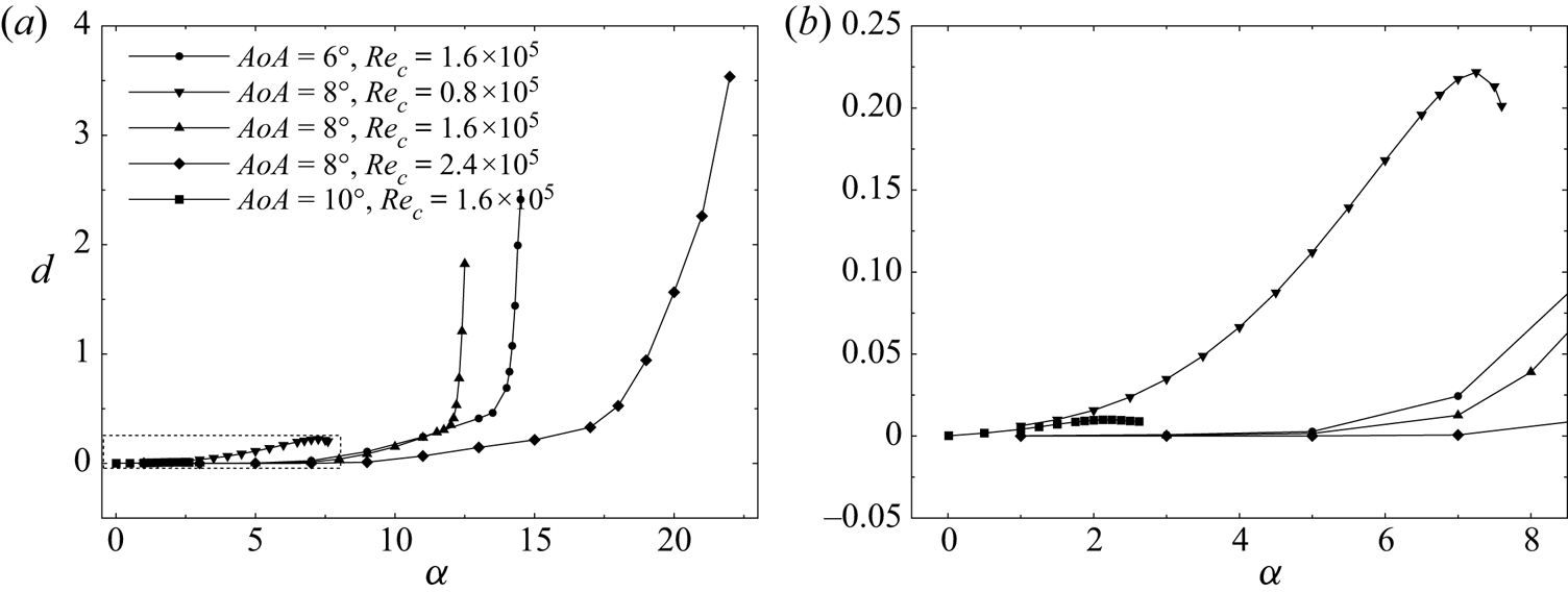
The penetration depth of the dominating Mode-A with positive- $m$ was inspected as a function of
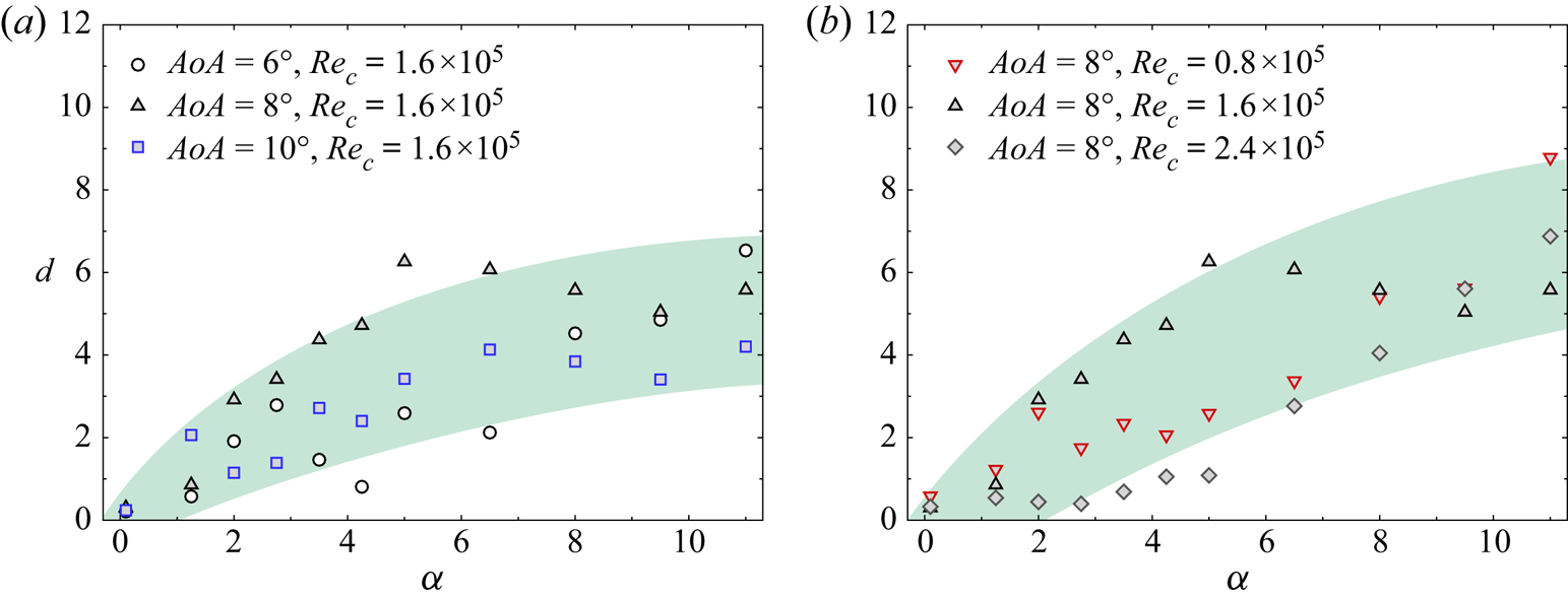
 $\alpha$ along the most amplified stability curve, as in figure 12. Figure 21 shows that the penetration depth enlarged significantly with increasing
 $\alpha$. For the unstable vortex at
 $[AoA, Re_c] = [6^{\circ }, 1.6\times 10^{5}; 8^{\circ }, 1.6\times 10^{5}; 8^{\circ }, 2.4\times 10^{5}]$, the penetration depth increased drastically after
 $\alpha$ exceeded a threshold. For the less unstable vortex of
 $AoA = 8^{\circ }, Re_c = 0.8\times 10^{5}$,
 $d$ increased with
 $\alpha$ but only mildly. For the vortex at
 $AoA = 10^{\circ }, Re_c = 1.6\times 10^{5}$, however,
 $d$ was maintained at approximately zero. A similar trend where the perturbation modes enlarge in size with increasing
 $\alpha$ was also observed by Fabre et al. (Reference Fabre, Sipp and Jacquin2006). However, Mode-A herein was found to transit in terms of its modal structure for large
 $\alpha$.
Penetration depth along the most amplified stability curve of the isolated vortex. (a) Penetration depth versus axial wavenumber, (b) a zoom-in view of the framed zone in (a) to show the small variation of  $d$ for
 $[AoA, Re_c] = [8^{\circ }, 0.8\times 10^{5}; 10^{\circ }, 1.6\times 10^{5}]$.

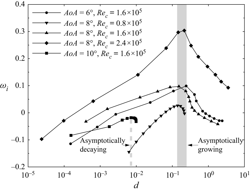
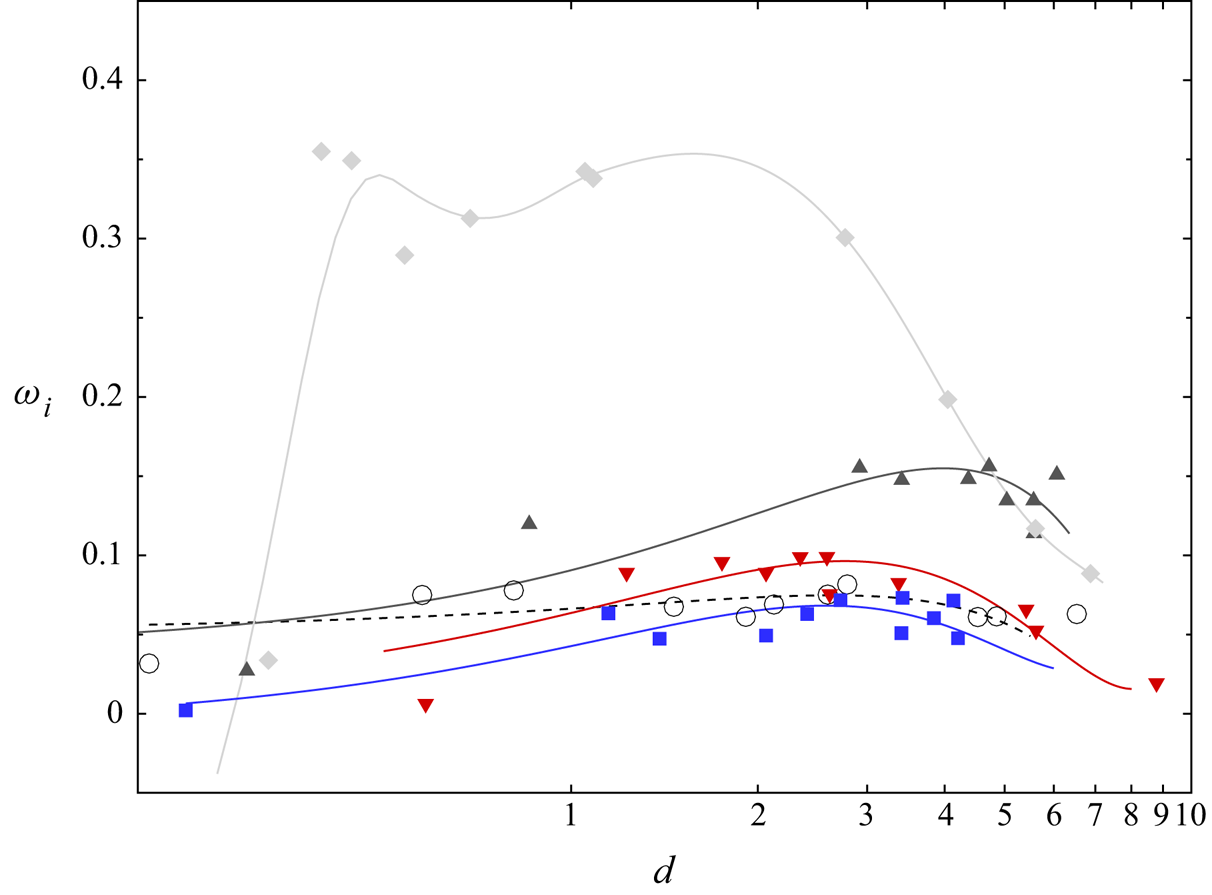
As the growth rate is a function of  $\alpha$, the nearly monotonic dependence of penetration depth on
 $\alpha$ infers that there should be a limiting penetration depth at which the perturbation amplifies the most. Figure 22 demonstrates
 $\omega _i$ as a function of
 $\alpha$. Notably, the growth rate of the four asymptotically unstable vortices peaked at an approximately identical penetration depth, which fell into a narrow band of
 $d = 0.14\sim 0.24$. The penetration depth corresponding to the neutrally stable vortex at
 $AoA = 10^{\circ }, Re_c = 1.6\times 10^{5}$, however, was below 0.01. The coincidence of the limiting
 $d$ for the four unstable trailing vortices is interesting as
 $d$ is indeed a rather sensitive parameter given its fractional form. A unified mechanism accounting for asymptotically unstable perturbations is hence expected to be underlying this specific parameter.
Variation of the growth rate with penetration depth for the isolated trailing vortex.

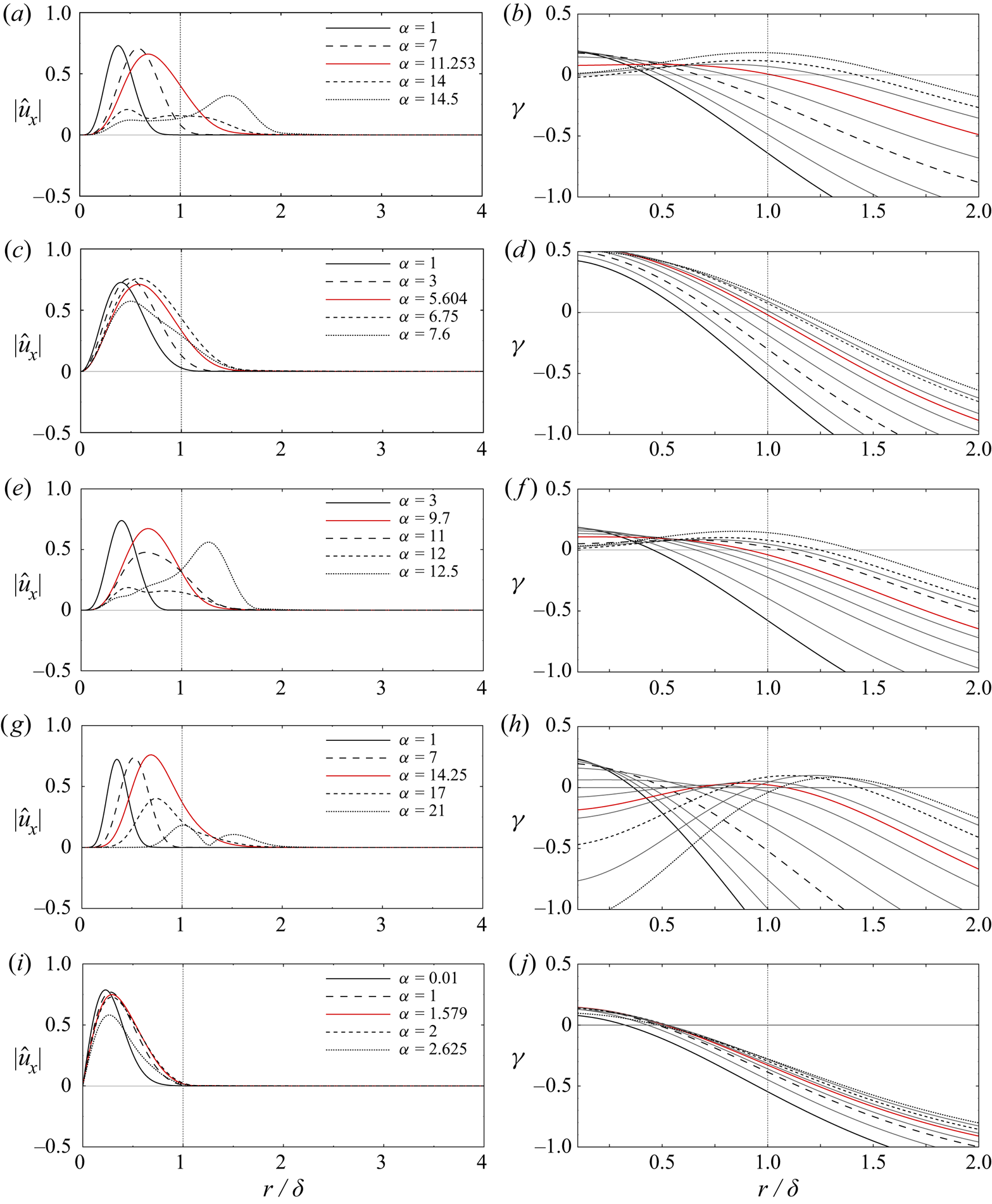
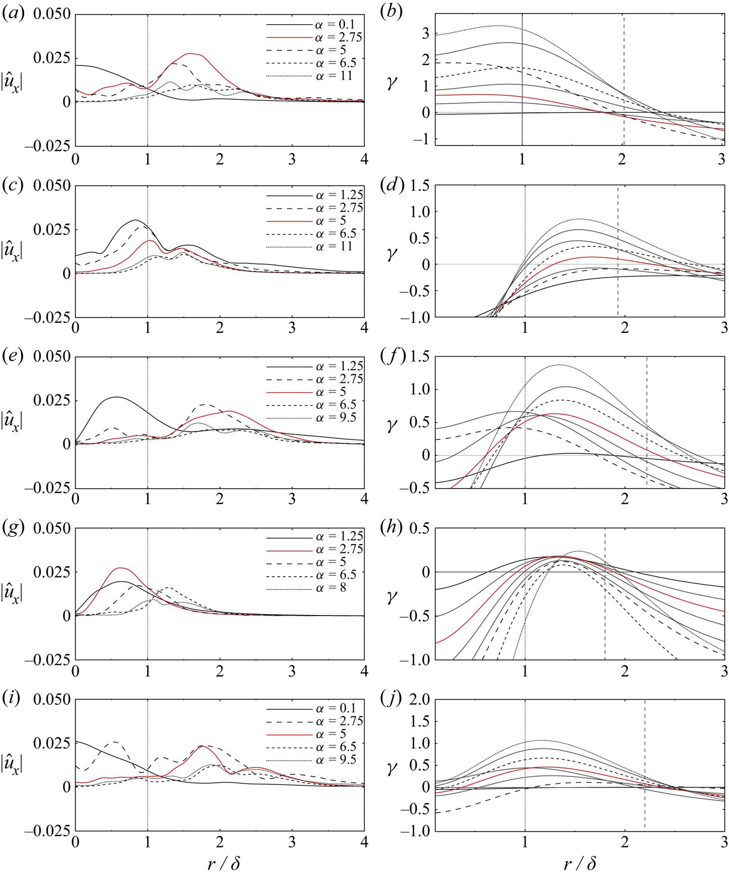
The existence of the limiting  $d$ was further illustrated in figure 23(a,c,e,g,i). As
 $\alpha$ increased, the perturbations corresponding to the four unstable cases (figure 23a,c,e,g) gradually spread over the core boundary where the vortex shear was located. The only exception was the case at
 $AoA=10^{\circ }, Re_c=1.6\times 10^{5}$, given the stable nature of its Mode-A. Notably, as the axial wavenumber continued to increase, perturbations in the four unstable cases convected away from the shear region, which is consistent with the dramatic increase of
 $d$ shown in figure 21. For the most-amplified modes in the four unstable cases, their relative locations with the core boundary were strikingly identical, which corresponded to the narrow band of limiting
 $d$ in figure 22. The limiting
 $d$ signified that there exists an extent of shear-penetration where the perturbations are most amplified. From the variation of perturbation with
 $\alpha$, as shown in figure 23, it was implied that there might be an optimal interaction between the perturbation and the vortex shear.
Mode variation with the axial wavenumber for the isolated trailing vortex: radial distribution of  $|\hat {u}_x|$ (a,c,e,g,i) and the corresponding
 $\gamma$ (b,d,f,h,j). The red curve corresponds to the most unstable perturbation. The critical point shifts continuously and the grey thin lines fill the gap in between, as shown in the right column for clearer illustration. The vertical line marks the core boundary. Flow conditions and azimuthal wavenumbers
 $[AoA, Re_c, m]$: (a,b)
 $[6^{\circ }, 1.6\times 10^{5}, 4]$, (c,d)
 $[8^{\circ }, 0.8\times 10^{5}, 2]$, (e,f)
 $[8^{\circ }, 1.6\times 10^{5}, 4]$, (g,h)
 $[8^{\circ }, 2.4\times 10^{5}, 6]$, (i,j)
 $[10^{\circ }, 1.6\times 10^{5}, 1]$.

The limiting  $d$ was then investigated by introducing the critical point in the trailing vortices. According to Lessen et al. (Reference Lessen, Singh and Paillet1974), the growth rate should be sensitive to the mean flow properties at this point. The critical point corresponds to the radial location
 $r$, where the azimuthal frequency
 $f_\theta$ and axial frequency
 $f_x$ of the perturbation cancel each other (Lessen et al. Reference Lessen, Singh and Paillet1974). The definition of a critical point is thus given by
 \begin{equation} \gamma^*=\alpha^* \left( U_x(r)-c \right)+mU_\theta(r)/r=0 \end{equation}
in which  $\gamma ^*$ is the local difference between
 $f_\theta$ and
 $f_x$, and
 $c=\omega ^*/\alpha ^*$ is the phase speed. The asterisk denotes a dimensional variable.
In the right column of figure 23, the  $\gamma$-curves correspond to the varying perturbations with increasing
 $\alpha$ as shown in the left column. The critical point is denoted by the zeros of the
 $\gamma$-curve, where
 $\gamma$ is non-dimensionalized by the reference time. Looking into the case at
 $AoA=6^{\circ }, Re_c=1.6\times 10^{5}$ as an example, as
 $\alpha$ increased, the critical point shifted away from the vortex centre. Below the critical point, the perturbation was featured by an excess of
 $f_\theta$ over
 $f_x$, where the flow experienced more azimuthal disturbances than axial disturbances. Comparing the left and right columns of figure 23, the peak of each mode was found to fall in the margin of
 $r < r_{cr}$ that pertained to the region of
 $f_\theta$-excess. The perturbation extended together with the region of
 $f_\theta$-excess and eventually permeated the core boundary as
 $\alpha$ increased. Furthermore, as the critical point shifted outward, the perturbation attained the maximum growth rates where the critical point coincided with the core boundary. The same was observed for the other three unstable cases, where the growth rate reached its maximum as the critical point approached the core boundary. However, the tendency for
 $AoA=10^{\circ }, Re_c=1.6\times 10^{5}$ was not evident as the perturbation was completely restricted in the vortex core and the shift of critical points was quite marginal. This was consistent with the stable nature of these perturbations. The correlation between the critical point and the vortex shear therefore highlights an interaction between the two characteristic layers of the
 $O(\epsilon )$ and the
 $O(1)$ flow. This interaction selects the dominating mode by the proximity of the critical point to the vortex shear layer.
6.2.2. Shear penetration for the co-rotating vortex pair
The interlink between the modal feature of perturbations and asymptotic instability was further examined for the co-rotating vortex pair. Figure 24 shows a similar increase of penetration depth versus axial wavenumber. As  $\alpha$ increased,
 $d$ uniformly increased beyond the scope of the core region. It should be noted that the variation of
 $d$ was very much complicated by the global nature of the vortex pair in which both
 $\omega$ and
 $m$ changed with
 $\alpha$. However, a general trend of
 $d$ increasing with
 $\alpha$ was still observed.
Penetration depth versus the streamwise wavenumber for the co-rotating vortex pair, (a) with different  $AoA$, (b) with different
 $Re_c$.

Figure 25 demonstrates that a limiting  $d$ also existed for each measured vortex pair at which the perturbation was most amplified. However, the limiting
 $d$ of the co-rotating vortex pair was larger than that of the isolated vortex, which reached up to
 $d > 1$. The left column of figure 26 illustrates the radial distribution of associated perturbation modes. Except for the vortex pair at
 $AoA=8^{\circ }, Re_c=2.4\times 10^{5}$, which pertained to a smaller limiting
 $d$, the perturbations permeated the core boundary completely as
 $\alpha$ increased. The perturbed regions for the co-rotating vortex pair were again associated with the shifting of the critical points, as shown in the right column of figure 26. The indication of the
 $f_\theta$-excess region favoured by the perturbations also held for the global scenario of the vortex pairs, as the peak of each global perturbation still resided in this region. As the
 $f_\theta$-excess region moved outward with the critical layer, the perturbations were shifted away accordingly.
Variation of the amplification rate with the penetration depth on a logarithmic scale. Symbols, data points from stability analysis; curves, polynomial fittings to show the trend of the data points. Here,  ${\bigcirc} , AoA=6^{\circ }, Re_c=1.6\times 10^{5}$;
 ${\blacktriangledown }$, red,
 $AoA=8^{\circ }, Re_c=0.8\times 10^{5}$;
 $\blacktriangle$,
 $AoA=8^{\circ }, Re_c=1.6\times 10^{5}$;
 ${\blacklozenge }$, grey,
 $AoA=8^{\circ }, Re_c=2.4\times 10^{5}$;
 ${\blacksquare }$, blue,
 $AoA=10^{\circ }, Re_c=1.6\times 10^{5}$.

Mode variation with the axial wavenumber for the co-rotating vortex pair. Dotted vertical line, the core boundary; dashed vertical line, the separatrix between the inner and outer recirculation zone as illustrated in Appendix C. Flow conditions  $[AoA, Re_c]$: (a,b)
 $[6^{\circ }, 1.6\times 10^{5}]$; (c,d)
 $[8^{\circ }, 0.8\times 10^{5}]$; (e,f)
 $[8^{\circ }, 1.6\times 10^{5}]$; (g,h)
 $[8^{\circ }, 2.4\times 10^{5}]$; (i,j)
 $[10^{\circ }, 1.6\times 10^{5}]$.

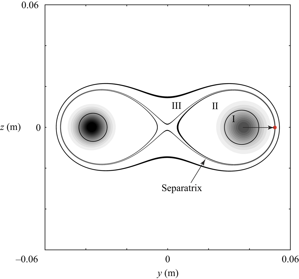
The relatively large value of limiting  $d$ for the co-rotating vortex pair is intriguing. In the right column of figure 26, the critical points were observed to also shift to larger radial locations than those of the isolated trailing vortex. Notably, for the isolated trailing vortex, only one shear layer existed which was located at the core boundary, while for co-rotating vortex pairs, an outer recirculation zone surrounded the two vortices where the fluid circulated as a whole. The recirculation zones for the co-rotating vortex pairs consisted of two core regions: two inner recirculation zones, where the fluid circulates the individual vortex, and an outer recirculation zone (see Appendix C). We found that the critical point of the most unstable perturbation in the vortex-pair scenario aligned with the radial position of the separatrix dividing the inner and outer recirculation zone. The radial position of the separatrix was determined by its outermost point (see figure 31). This particular layer of the co-rotating vortex pair separated the fluid rotating about each vortex centre from that circulating both the vortices. This layer therefore formed a mutual shear layer of the vortex pair in addition to the shear layer at the individual core boundary. Analogous to the isolated vortex scenario, the alignment between the critical point of the most unstable perturbation and the separatrix pointed to an interaction between the two characteristic layers of the
 $O(\epsilon )$ perturbation field and the
 $O(1)$ base flow. The perturbation was amplified in the asymptotic limit as its critical point moved toward the mutual shear of the vortex pair. The results from the vortex pair scenario further substantiated that the asymptotic growth of instability is associated with an interplay between the critical points of the perturbations and the corresponding characteristic layer of the base flow.
6.3. Discussion on the interplay between the perturbation and base flow
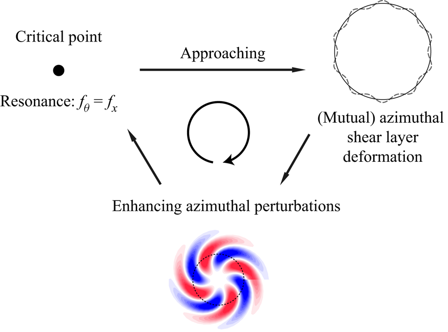
The analysis above points to an interlink between the critical point, the base flow shear and the asymptotic growth of perturbations. Figure 27 illustrates such interplay between the perturbation and the base flow. At the critical point, the fluid experiences equal number of azimuthal and axial disturbances. A resonance is thus produced at this point between the azimuthal and axial waves. Subject to the associated dispersion relation, the critical point shifts in the  $O(1)$ flow, as shown in figures 23 and 26. As the critical point approaches the core boundary, this resonance is likely to cause deformation of the azimuthal shear layer and perturb the
 $O(1)$ base flow. A similar deformation of the vortex core induced by perturbations has been observed by Hattori, Blanco-Rodríguez & Le Dizès (Reference Hattori, Blanco-Rodríguez and Le Dizès2019) in a vortex ring with swirl, and according to Fabre et al. (Reference Fabre, Sipp and Jacquin2006), there is an exchange of energy between the base flow and the perturbation wave owing to a resonance at the critical layer. The perturbed flow thus in turn enhances the azimuthal perturbation at
 $O(\epsilon )$, which is found to dominate instability. A similar interaction exists for the co-rotating vortex pairs, where instability is amplified through the interplay between the critical point and the mutual shear layer at the separatrix between the inner and outer recirculation zones. The interaction with the mutual shear layer amplifies the global perturbation. This is probably because the mutual shear layer transfers disturbances between the two vortices, whereas the inner shear only affects the individual vortex. In both of the vortex configurations, however, it can be commented that the asymptotic growth of perturbations is achieved by the interaction between the characteristic layers of the
 $O(\epsilon )$ and
 $O(1)$ flow fields.
Graphic description of the mechanism for asymptotic growth in trailing vortices: interaction between the  $O(\epsilon )$ perturbations and the
 $O(1)$ base flow.

7. Conclusion
In this paper, we focus on the asymptotic instability of two canonical vortex systems, namely an isolated vortex and a co-rotating vortex pair with axial flow, to investigate the characteristics of their linear perturbations and to understand the mechanism for these perturbations to undergo asymptotic growth/decay. The basic state and vortex wandering of the two vortex configurations are captured by SPIV experiments. Based on the measured flow field, local and global stability analyses were carried out to acquire the instability characteristics of the two vortex configurations.
For the isolated trailing vortex, perturbations that counter vortex rotation ( $m>0$) and rotate with the vortex (
 $m<0$), as well as an axisymmetric perturbation (
 $m = 0$), are identified. Mode-A with positive-
 $m$ is found to be asymptotically unstable, while Mode-A with negative-
 $m$ is substantially damped. Mode-A with positive-
 $m$ manifests a spiral, azimuthal structure which extends outside the vortex core, while Mode-A with negative-
 $m$ is strictly confined by the core boundary. The discrete mode in the P-family (Mode-P) is an axisymmetric or dipole structure (
 $|m|\leqslant 1$), which is neutrally stable. The measured trailing vortex conforms to Leibovich & Stewartson's asymptotic theory (Reference Leibovich and Stewartson1983) where perturbations are clustered at a critical radius.
In the co-rotating vortex pair, a similar azimuthal perturbation is found to be asymptotically unstable, which pertains to the upper vortex (Mode-U). The wavelength is of the same order as the core radius, which suggests that the mode is short-wave in nature. For the lower vortex, the perturbation is radial (Mode-L). The upper vortex is more disturbed than the lower vortex, as Mode-U overwhelms Mode-L with a higher growth rate. This difference is supported by the measured wandering amplitude where the upper vortex manifests stronger oscillation. The  $(-1, 1)$ and
 $(-2, 0)$ modes are found to exist in the measured vortex configuration but are of a lower growth rate than the dominating perturbation.
For both the isolated trailing vortex and the co-rotating vortex pair, the perturbations dominating in the asymptotic limit manifest identical features with azimuthal components penetrating the core boundary. The perturbation attains the maximum growth rate at a limiting value of the penetration depth through the vortex shear,  $d=[0.14, 0.24]$ for the isolated vortex and
 $d > 1$ for the co-rotating vortex pair. Furthermore, the asymptotic growth of perturbations is ascribed to an alignment between their critical points and the characteristic layers of the base flows for both vortex configurations. For the isolated vortex, the growth rate maximizes as the critical point approaches the shear layer at the core boundary. For the vortex pair, the global perturbation is most amplified when its critical point moves toward the mutual shear layer at the separatrix between the inner and outer circulation zones. This interplay between the characteristic layers of the
 $O(\epsilon )$ perturbation and the
 $O(1)$ flow field gives rise to the asymptotic growth of perturbations in trailing vortices.
The results above point to an underlying correlation between the asymptotic instability and the modal structure of perturbations in trailing vortices, which will help guide the design of physical-based flow control methods to render the instability of such swirling flows. Validation for the effectiveness of this potential strategy to modify the instability by leveraging the modal structure of perturbations is desired for future applications.
Acknowledgements
The authors would like to thank Dr Suyang Qin for the discussion and help during the setup of the experiment and Dr Linying Li for the enthusiastic discussions during the implementation of the stability analysis, as well as the reviewers for a number of constructive suggestions on the manuscript.
Funding
Financial support from the State Key Development Program of Basic Research of China (2014CB744802) is gratefully acknowledged. Furthermore, this work was also supported by NSFC Projects (91941301; 91952302) and China Postdoctoral Science Foundation (2018M642007).
Declaration of interests
The authors report no conflict of interest.
Appendix A. Stability matrices and mapping functions
A.1. Local stability matrices
The stability matrices for the local problem of  $\boldsymbol{\mathsf{A}}_{\boldsymbol{g}}\hat {\boldsymbol{q}}=\omega \boldsymbol{\mathsf{B}}_{\boldsymbol{g}}\hat {\boldsymbol{q}}$ is given as
 \begin{equation} \boldsymbol{\mathsf{A}}_{\boldsymbol{g}} = \left[ \begin{array}{cccc} {{D_y} + \dfrac{1}{r}} & {\dfrac{m}{r}} & \alpha & 0\\ {{L_1}} & {\dfrac{{\textrm{i}2m}}{{{r^2}Re}} - \dfrac{{2{{\bar{u}}_\theta }}}{r}} & 0 & {{D_y}}\\ {\textrm{i}{D_y}{{\bar u}_\theta } + \dfrac{{2m}}{{{r^2}Re}} + \dfrac{{\textrm{i}{{\bar u}_\theta }}}{r}} & {{L_2}} & 0 & {\dfrac{{\textrm{i}m}}{r}}\\ {\textrm{i}{D_y}{{\bar u}_x}} & 0 & {{L_3}} & {\textrm{i}\alpha } \end{array}\right],\quad \boldsymbol{\mathsf{B}}_{\boldsymbol{g}} =\left[ \begin{array}{cccc} 0 & 0 & 0 & 0\\ { - 1} & 0 & 0 & 0\\ 0 & i & 0 & 0\\ 0 & 0 & i & 0 \end{array}\right] \end{equation}
with
 \begin{gather} {L_1} ={-} \frac{\textrm{i}}{{Re}}D_{yy}^2 + \textrm{i}\left({\bar u_r} - \frac{1}{{rRe}}\right){D_y} + \left[\textrm{i}{D_y}{\bar u_r} - \frac{{m{{\bar u}_\theta }}}{r} - \alpha {\bar u_x} + \frac{\textrm{i}}{{Re}}\left(\frac{{{m^2} + 1}}{{{r^2}}} + {\alpha ^2}\right)\right] \end{gather}
 \begin{gather}{L_2} ={-} \frac{1}{{Re}}D_{yy}^2 + \left({\bar u_r} - \frac{1}{{rRe}}\right){D_y} + \left[\textrm{i}\frac{{m{{\bar u}_\theta }}}{r} + \textrm{i}\alpha {\bar u_x} + \frac{{{{\bar u}_r}}}{r} + \frac{1}{{Re}}\left(\frac{{{m^2} + 1}}{{{r^2}}} + {\alpha ^2}\right)\right] \end{gather}
 \begin{gather}{L_3} ={-} \frac{1}{{Re}}D_{yy}^2 + \left({\bar u_r} - \frac{1}{{rRe}}\right){D_y} + \left[\textrm{i}\frac{{m{{\bar u}_\theta }}}{r} + \textrm{i}\alpha {\bar u_x} + \psi + \frac{1}{{Re}}\left(\frac{{{m^2}}}{{{r^2}}} + {\alpha ^2}\right)\right] \end{gather}
in which  $D_y$ and
 $D_{yy}$ are the first-order and second-order Chebyshev differential operators in the radial direction, and
 $\psi$ is the streamwise gradient of
 $\bar {u}_x$, which is taken to be zero herein. Details of the boundary conditions are provided by Khorrami et al. (Reference Khorrami, Malik and Ash1989), so are omitted here for brevity.
A.2. Global stability matrices
The stability matrices for the global problem of  ${\boldsymbol{\mathsf{A}}_{\boldsymbol{g}}\hat {\boldsymbol{q}}}=\omega \boldsymbol{\mathsf{B}}_{\boldsymbol{g}}\hat {\boldsymbol{q}}$ is given as
 \begin{equation} {\boldsymbol{A}_{g}} = \left[ \begin{array}{cccc} {{L_T}} & {{U_y}} & {{U_z}} & {\textrm{i}\alpha }\\ 0 & {{L_T} + {V_y}} & {{V_z}} & {{D_y}}\\ 0 & {{W_y}} & {{L_T} + {W_z}} & {{D_z}}\\ {\textrm{i}\alpha } & {{D_y}} & {{D_z}} & 0 \end{array}\right],\quad {\boldsymbol{B}_{g}} = \left[ \begin{array}{cccc} \textrm{i} & 0 & 0 & 0\\ 0 & \textrm{i} & 0 & 0\\ 0 & 0 & \textrm{i} & 0\\ 0 & 0 & 0 & 0 \end{array} \right]\end{equation}
with  ${L_T} = \textrm {i}\alpha U + V{D_y} + W{D_z} - {1}/{{{{Re}}}}(D_y^2 + D_z^2 - {\alpha ^2})$. The two-dimensional Chebyshev differential matrices
 $D_y$ and
 $D_z$ resolve the derivatives along the
 $y$- and
 $z$-directions, respectively (Paredes Reference Paredes2014). The boundary conditions are
 $\hat {u}=\hat {v}=\hat {w}=0$ in the far-field and a compatibility condition for
 $\hat {p}$ derived from the N–S equation, as reported by Theofilis et al. (Reference Theofilis, Duck and Owen2004). Only temporal analysis is performed in the present study, whereas a detailed application of spatial bi-global analysis to trailing vortices is reported by He et al. (Reference He, Tendero, Paredes and Theofilis2017).
A.3. Mapping functions
For the vortex pair, the Chebyshev points should be mapped onto a two-dimensional domain. As the two vortices are separated by a distance, it is desirable to resolve both the vortex cores and the margin in between. Therefore, a mapping function is constructed herein to extend the refined region along the  $y$-direction and to resolve both the vortex cores clearly, which reads,
 \begin{equation} \left.\begin{gathered} y=C_{1} \left( a\eta_M-\frac{a^{3}\eta_M^{3}}{6}+\frac{a^{5}\eta_M^{5}}{C_2} \right)\\ \eta_M=\frac{{\beta}L\tan(k_y{\rm \pi}\eta/2)}{\tan(k_y{\rm \pi}/2)},\quad a={\rm \pi}/L \end{gathered}\right\} \end{equation}
where  $\eta _i=\cos ({{\rm \pi} }i/N_Y),i=0,1,\ldots ,N_Y$ denotes the Chebyshev points in the y-direction, and the other parameters are adjustable for tuning of the refined region. For the z-direction, the mesh only needs refinement around
 $z = 0$ so the conventional mapping as in Hein & Theofilis (Reference Hein and Theofilis2004) and Edstrand et al. (Reference Edstrand, Schmid and Taira2018a) is employed herein. The mapping function applied in the local analysis is reported by Malik, Zang & Hussaini (Reference Malik, Zang and Hussaini1985).
Appendix B. Validation with a equal-strength co-rotating vortex pair
B.1. Validation of the numerical methods
The validation result of the local stability analysis is presented in table 3 and of the global analysis in figure 28. A convergence study for both methods is shown in table 4.
Validation of the bi-global stability code. Top row: duct flow (Theofilis et al. Reference Theofilis, Duck and Owen2004); aspect ratio (a1)  $A = 1$, (b1)
 $A = 4$. Bottom row: (a2) isolated Batchelor vortex and (b2) counter-rotating vortex pair (Hein & Theofilis Reference Hein and Theofilis2004). Black dots, results from the present code; red circles, results in the literature.

Validation of the present method for different shear flows against Khorrami et al. (Reference Khorrami, Malik and Ash1989) and Fabre & Jacquin (Reference Fabre and Jacquin2004).

Convergence study of the present method for the  $q$-vortex of Mayer & Powell (Reference Mayer and Powell1992),
 $q = 0.475$.

B.2. Validation with an equal-strength co-rotating vortex pair
To further validate the implementation of bi-global analysis applied in the present study, we reproduced the instability mode of an equal-strength co-rotating vortex pair with zero axial flow at the same parameters of  $Re = \varGamma /\nu = 14000, \delta /b = 0.14$ as reported in Roy et al. (Reference Roy, Schaeffer, Le Dizés and Thompson2008) by using our bi-global code. The EVP (A5a,b) in Appendix A.1 was solved and the equations were non-dimensionalized by
 $\delta$ and
 $U_c = \varGamma /(2{\rm \pi} \delta )$.
Two modes with the largest growth rate, which correspond to  $\alpha = 2$ and
 $\alpha = 3.5$ according to Roy et al. (Reference Roy, Schaeffer, Le Dizés and Thompson2008), were chosen for the validation of our bi-global codes. These were the modes of
 $(m_1, m_1, n) = (-1,1,1)$ and
 $(-1,1,2)$ at
 $\alpha = 2$ and
 $\alpha = 3.5$, respectively;
 $n$ denotes the radial complexity within the vortex core. In our computation,
 $64^2$ Chebyshev points were used to discretize the base flow (figure 29) by applying the mapping function described in Appendix A.3. By solving the discretized equation (A5a,b), two eigenmodes were identified and their modal structures are presented in figure 30. The
 $(-1,1,1)$ and
 $(-1,1,2)$ modes were resolved by the bi-global code at
 $\alpha = 2.0$ and
 $\alpha = 3.5$, respectively. Despite a relatively low resolution, the azimuthal wavenumber of the Kelvin modes and the radial wavenumber were captured for each mode. The results showed a good agreement between the perturbation mode obtained by our bi-global code and that computed by Roy et al. (Reference Roy, Schaeffer, Le Dizés and Thompson2008).
Base flow of the equal-strength co-rotating vortex pair and the Chebyshev grid to discretize the domain,  $(Ny, Nz)=(64, 64)$. The contour shows the axial vorticity; the black curve shows the stream line.

Perturbation modes obtained by the present bi-global code and those reported by Roy et al. (Reference Roy, Schaeffer, Le Dizés and Thompson2008) for an equal-strength co-rotating vortex pair with the same parameters.

Appendix C. Recirculation zones of the co-rotating vortex pair
In the non-comoving reference frame, which is fixed to the wind tunnel, the fluid circulating the co-rotating vortex pair can be divided into three zones, as shown in figure 31. Zone I is the individual core region; Zone II is the inner recirculation zone where the fluid circulates solely one vortex; Zone III is the outer recirculation zone where the fluid travels around both vortices. Therefore, a separatrix of the inner and outer recirculation zones exists which divides the fluid circulating one vortex from that circulating both. A mutual shear layer therefore lies at this separatrix. It is demonstrated in § 6 that the separatrix interacts with the critical points and leads to asymptotic instability growth in the co-rotating vortex pairs.
Recirculation zones of the co-rotating vortex pair. I. core region; II. inner recirculation zone; III. outer recirculation zone. The contour shows the axial vorticity. The red dot denotes the outermost point of the separatrix between II and III.