1 Introduction
The most distinctive features of supersonic flows are shock waves. Linear shock waves, such as normal shocks and oblique shocks, are a fundamental aspect of fluid mechanics and the associated theories are now well established. However, although analytical studies of curved shock waves began a long time ago, this field is still in the process of development. In early studies, Crocco (Reference Crocco1937) discovered the Crocco point, at which the post-shock flow curvature is equal to zero, and Thomas (Reference Thomas1947) found the Thomas point, which is used to identify compressive and expansive flow fields. In the following years, much effort was focused on shock curvature and flow parameter gradients. On the basis of the work by Crocco (Reference Crocco1937) and Thomas (Reference Thomas1947), Lin & Rubinov (Reference Lin and Rubinov1948) showed that a normal shock can attach to a continuously curved boundary only at a certain Mach number. Thomas (Reference Thomas1949) presented detailed profiles of the streamline curvature behind curved shocks in planar flow. Kanwal (Reference Kanwal1959) obtained solutions for the streamwise gradients of flow parameters on the downstream side of a three-dimensional shock. Hayes & Probstein (Reference Hayes and Probstein1959) extended these works to the relevant normal derivatives in the close neighbourhood of a spherically shaped (axisymmetric) shock. Gerber & Bartos (Reference Gerber and Bartos1960) derived the curved shock equation coefficients assuming that the oncoming flow is steady, irrotational and uniform. These coefficients can be applied to locate the initiation point of constant-property lines at planar and axisymmetric shock waves. Hornung (Reference Hornung1998) presented the shock-normal derivatives for the inviscid equations of motion of a curved shock, taking account of real-gas effects. A number of investigations of the jump conditions and the tangential and normal derivatives of common flow characteristics were performed, although the effects of vorticity were not considered until, on the basis of the equation of state and Crocco’s thermodynamic relation, Truesdell (Reference Truesdell1952) was able to derive the vorticity function through a curved shock wave in planar flow, and Kanwal (Reference Kanwal1959) presented five conditions for the vorticity to vanish behind the shock surface. Much later, Emanuel (Reference Emanuel1988) developed a general theory to determine the tangential and normal derivatives of properties just downstream of a curved, unsteady shock wave and presented a modern treatment of curved shocks based on a vector calculus approach (Emanuel Reference Emanuel2012).
Although many aspects of shock waves have been investigated over the years, most research has been concerned with incident shocks. However, reflection is also an essential phenomenon that occurs with shock waves. Pant (Reference Pant1971) analysed the regular reflection of a curved shock from a straight rigid boundary and presented a relation between the curvatures of the incident and reflected shocks. Ivanov (Reference Ivanov1995) described a hysteresis effect arising in stationary reflection of shock waves. Christopher (Reference Christopher2008) presented an experimental illustration of the mechanism by which transition between regular and Mach reflection is induced. Wang (Reference Wang2017) observed the phenomena of both regular reflection and Mach reflection by adjusting the initial wedge angle. Mölder (Reference Mölder2017b) solved the regular reflection and Mach reflection flow fields near planar and axisymmetric curved shocks and compared the theoretical results with numerical calculations and experiments. Earlier, Mölder (Reference Mölder1972) had investigated the pressure/deflection polar for Mach reflection and obtained some important compatibility relations for the streamline direction across the slip layer. It should be noted that most of the above studies were based on calorically and thermally perfect flows.
Most derivations have been confined to curved shocks that possess only a single shock curvature. This restriction has narrowed the range of applications of curved shock theory because in most situations of interest shock waves are doubly curved. Furthermore, the incoming flows are generally non-uniform and rotational. To widen the scope of the theory, Mölder (Reference Mölder2015) derived curved shock equations by taking account of vorticity as well as non-uniformity and compound shock curvature. Theoretically, these equations can be used for three-dimensional flow. However, they are subject to the restriction that the flow plane must coincide with the osculating plane, as in the case of the symmetry plane of an elliptical conical flow field at zero angle of attack. Although the derivation and its results are complicated, the equations can be applied in subsonic flow regions, in contrast to the method of characteristics, which can only be used for supersonic flow fields. In addition, expressions in an influence coefficient form have been derived and applied to analyse the effects of various pre-shock parameters on post-shock variables. This extended curved shock theory can be used to illuminate many important phenomena of shock wave dynamics from a unique perspective. Furthermore, the theory is applicable not only to uniform flow, but also to non-uniform flow both upstream and downstream of a doubly curved shock surface. A novel derivation of post-shock vorticity based on the theory has also been presented, in which the effects of pre-shock flow non-uniformities and flow divergence on post-shock vorticity are taken into account. Curved shock theory has contributed greatly to the development of shock wave research. Based on this theory, Uskov & Mostovykh (Reference Uskov and Mostovykh2016) gave the flow gradients in the vicinity of a shock wave for a thermodynamically imperfect gas. Mölder (Reference Mölder2017a) applied curved shock theory to concave shock waves in a study of reflection and obtained a relation between shock curvature ratio and shock reflection. Emanuel (Reference Emanuel2018) extended curved shock theory to unsteady flow and an imperfect gas. On the basis of curved shock theory, Filippi & Skews (Reference Filippi and Skews2018) used streamlines behind axisymmetric curved shock waves to predict the internal surfaces that produced these streamlines.
Furthermore, since curved shock theory gives a connection between shock curvature and flow parameters, it can be extended to capture shock shape. Moretti & Abbett (Reference Moretti and Abbett1966) and Moretti & Salas (Reference Moretti and Salas1970) fitted a shock wave under the hypothesis that the wave was a surface of discontinuity and the physical parameters should be compatible with the Rankine–Hugoniot equations. This method was then widely applied to numerical computation of hypersonic flows. However, the information acquired by the Rankine–Hugoniot equations is limited. For high-precision shock wave fitting, a higher-order theory is required. The advantage of curved shock theory in acquiring high-order variables to describe shock geometry makes this theory a good candidate for solving shock capture problems in computational fluid dynamics algorithms. For broader applications such as the acquisition of higher-order physical information, first-order derivatives are insufficient. However, modern computer algebra manipulators make it possible to derive higher-order derivatives.
In this paper, second-order curved shock equations are derived that relate shock curvature gradients directly to the second-order gradients of flow properties near the shock. These equations are obtained by taking derivatives of both sides of each of the curved shock equations and can be utilized for a doubly curved shock in steady flow where the upstream flow can have a second-order pressure gradient, a streamline curvature gradient and a vorticity gradient. An influence coefficient formulation of the second-order curved shock equations is also derived and used to study the relations between pre- and post-shock variables. Given some hypotheses, the equations can be used efficiently to obtain approximate solutions for the flow field behind a curved shock. They can also be applied to shock wave fitting by solving for the shock curvature gradients.
2 Derivation of second-order curved shock theory
Second-order curved shock theory is developed on the basis of conventional curved shock theory. For clarity, in this paper, the latter theory is termed first-order curved shock theory to distinguish it from the second-order theory and is introduced before the second-order curved shock equations are derived. The first-order equations were originally derived by Mölder (Reference Mölder2015). Although all the equations in the present paper are either newly derived or rederived, the methodology and nomenclature follow those of Mölder.
2.1 Introduction to the first-order curved shock equations
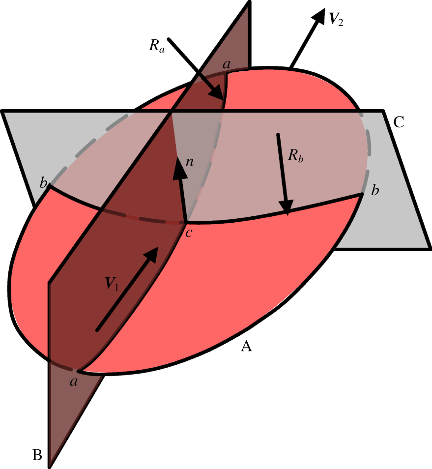
The geometry of a curved shock A in supersonic flow is shown in figure 1. The flow passes through the shock wave with an incoming velocity vector  $\boldsymbol{V}_{1}$ and a leaving velocity vector
 $\boldsymbol{V}_{2}$, which define the flow plane B. The flow-normal plane C, which is perpendicular to the shock wave and the flow plane, has a trace
 $b{-}b$ in the shock wave. The intersection line
 $a{-}a$ of the flow plane and shock wave has an intersection point
 $c$ with the trace
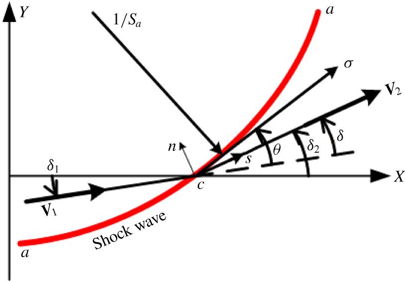
 $b{-}b$. The Cartesian coordinate system lies in the flow plane. The velocity angles
 $\unicode[STIX]{x1D6FF}_{1}$ and
 $\unicode[STIX]{x1D6FF}_{2}$ in figure 2 are the acute angles between the velocity vectors and the
 $X$ axis, so the flow deflection angle
 $\unicode[STIX]{x1D6FF}$ is calculated as
 $\unicode[STIX]{x1D6FF}=\unicode[STIX]{x1D6FF}_{2}-\unicode[STIX]{x1D6FF}_{1}$. Similarly, the shock angle
 $\unicode[STIX]{x1D703}$ is defined as the angle by which the line
 $a{-}a$ is inclined to the incoming velocity vector
 $\boldsymbol{V}_{1}$. The length
 $\unicode[STIX]{x1D70E}$ is the distance measured along the trace
 $a{-}a$. The lengths
 $s$ and
 $n$ are the distances measured respectively along and perpendicular to the streamline. Based on these variables, the variable
 $S_{a}$, which represents the curvature of the shock wave in the flow plane, is given by
 $S_{a}=-1/R_{a}=\unicode[STIX]{x2202}\unicode[STIX]{x1D703}_{1}/\unicode[STIX]{x2202}\unicode[STIX]{x1D70E}$. In like manner, the curvature of the shock wave in the flow-normal plane is
 $S_{b}=-1/R_{b}=-\cos \unicode[STIX]{x1D703}_{1}/y$, where
 $y$ is the distance from the shock wave to the
 $X$ axis.
Geometry of curved shock from Mölder (Reference Mölder2015).

Variables in the flow plane.

For clarity in the derivation of the first-order curved shock equations, Mölder introduced the following normalized variables.
 $$\begin{eqnarray}\displaystyle \text{normalized pressure gradient:} & & \displaystyle P=(\unicode[STIX]{x2202}p/\unicode[STIX]{x2202}s)/\unicode[STIX]{x1D70C}V^{2},\nonumber\\ \displaystyle \text{streamline curvature:} & & \displaystyle D=\unicode[STIX]{x2202}\unicode[STIX]{x1D6FF}/\unicode[STIX]{x2202}s,\nonumber\\ \displaystyle \text{normalized vorticity:} & & \displaystyle \unicode[STIX]{x1D6E4}=\unicode[STIX]{x1D714}/V.\nonumber\end{eqnarray}$$
In terms of these variables, the Euler equations for steady flow then take the form
 $$\begin{eqnarray}\displaystyle & \text{mass:} & \displaystyle \qquad \frac{\unicode[STIX]{x2202}\unicode[STIX]{x1D6FF}}{\unicode[STIX]{x2202}n}=-(Ma^{2}-1)P-j\frac{\sin \unicode[STIX]{x1D6FF}}{y},\end{eqnarray}$$
 $$\begin{eqnarray}\displaystyle & s\text{-momentum:} & \displaystyle \qquad \frac{1}{V}\frac{\unicode[STIX]{x2202}V}{\unicode[STIX]{x2202}s}=-\frac{1}{\unicode[STIX]{x1D70C}V^{2}}\frac{\unicode[STIX]{x2202}p}{\unicode[STIX]{x2202}s}=-P,\end{eqnarray}$$
 $$\begin{eqnarray}\displaystyle & n\text{-momentum:} & \displaystyle \qquad \frac{1}{\unicode[STIX]{x1D70C}V^{2}}\frac{\unicode[STIX]{x2202}p}{\unicode[STIX]{x2202}n}=-\frac{\unicode[STIX]{x2202}\unicode[STIX]{x1D6FF}}{\unicode[STIX]{x2202}s}=-D,\end{eqnarray}$$
 $$\begin{eqnarray}\displaystyle & \text{energy:} & \displaystyle \qquad \frac{1}{\unicode[STIX]{x1D70C}}\frac{\unicode[STIX]{x2202}\unicode[STIX]{x1D70C}}{\unicode[STIX]{x2202}n}=-Ma^{2}[D+(\unicode[STIX]{x1D6FE}-1)\unicode[STIX]{x1D6E4}],\nonumber\\ \displaystyle & \quad & \displaystyle \qquad \frac{1}{\unicode[STIX]{x1D70C}}\frac{\unicode[STIX]{x2202}\unicode[STIX]{x1D70C}}{\unicode[STIX]{x2202}s}=Ma^{2}P,\end{eqnarray}$$
 $$\begin{eqnarray}\displaystyle & \text{vorticity:} & \displaystyle \qquad \frac{1}{V}\frac{\unicode[STIX]{x2202}V}{\unicode[STIX]{x2202}n}=D-\unicode[STIX]{x1D6E4}.\end{eqnarray}$$
In these equations, all variables have subscript either 1 or 2 depending on whether the application is to flow before or after the shock. The variable  $y$ does not need a subscript, since it has the same value for states 1 and 2 on opposite sides of the same shock. The use of
 $j$ to indicate flow with planar or axial symmetry will not be carried any further here. Applying these relations to the Rankine–Hugoniot equations
 $$\begin{eqnarray}\displaystyle & \displaystyle \frac{p_{2}}{p_{1}}=\frac{2\unicode[STIX]{x1D6FE}}{\unicode[STIX]{x1D6FE}+1}Ma_{1}^{2}\sin ^{2}\unicode[STIX]{x1D703}-\frac{\unicode[STIX]{x1D6FE}-1}{\unicode[STIX]{x1D6FE}+1}, & \displaystyle\end{eqnarray}$$
 $$\begin{eqnarray}\displaystyle & \displaystyle p_{1}+\unicode[STIX]{x1D70C}_{1}V_{1}^{2}\sin ^{2}\unicode[STIX]{x1D703}=p_{2}+\unicode[STIX]{x1D70C}_{2}V_{2}^{2}\sin ^{2}(\unicode[STIX]{x1D703}-\unicode[STIX]{x1D6FF}) & \displaystyle\end{eqnarray}$$
produces (after a few pages of algebraic manipulation) the first-order curved shock equations
 $$\begin{eqnarray}\displaystyle & \displaystyle A_{1}P_{1}+B_{1}D_{1}+E_{1}\unicode[STIX]{x1D6E4}_{1} & \displaystyle =A_{2}P_{2}+B_{2}D_{2}+CS_{a}+GS_{b},\end{eqnarray}$$
 $$\begin{eqnarray}\displaystyle & \displaystyle A_{1}^{\prime }P_{1}+B_{1}^{\prime }D_{1}+E_{1}^{\prime }\unicode[STIX]{x1D6E4}_{1} & \displaystyle =A_{2}^{\prime }P_{2}+B_{2}^{\prime }D_{2}+C^{\prime }S_{a}+G^{\prime }S_{b},\end{eqnarray}$$
where
 $$\begin{eqnarray}\left.\begin{array}{@{}c@{}}A_{1}=2\cos \unicode[STIX]{x1D703}\,[(3Ma_{1}^{2}-4)\sin ^{2}\unicode[STIX]{x1D703}-(\unicode[STIX]{x1D6FE}-1)/2]/(\unicode[STIX]{x1D6FE}+1),\\ B_{1}=2\sin \unicode[STIX]{x1D703}\,[(\unicode[STIX]{x1D6FE}-5)/2+(4-Ma_{1}^{2})\sin ^{2}\unicode[STIX]{x1D703}]/(\unicode[STIX]{x1D6FE}+1),\\ E_{1}=-2\sin ^{3}\unicode[STIX]{x1D703}\,[2+(\unicode[STIX]{x1D6FE}-1)Ma_{1}^{2}]/(\unicode[STIX]{x1D6FE}+1),\\ A_{2}=\sin \unicode[STIX]{x1D703}\cos \unicode[STIX]{x1D703}/\text{sin}\,(\unicode[STIX]{x1D703}-\unicode[STIX]{x1D6FF}),\\ B_{2}=-\sin \unicode[STIX]{x1D703}\cos \unicode[STIX]{x1D703}/\text{cos}\,(\unicode[STIX]{x1D703}-\unicode[STIX]{x1D6FF}),\\ C=-4\sin \unicode[STIX]{x1D703}\cos \unicode[STIX]{x1D703}/(\unicode[STIX]{x1D6FE}+1),\\ G=4\sin ^{2}\unicode[STIX]{x1D703}\cos \unicode[STIX]{x1D703}\sin \unicode[STIX]{x1D6FF}_{1}/[(\unicode[STIX]{x1D6FE}+1)\cos \unicode[STIX]{x1D703}_{1}],\end{array}\right\}\end{eqnarray}$$
and
 $$\begin{eqnarray}\left.\begin{array}{@{}c@{}}A_{1}^{\prime }=Ma_{1}^{2}\cos ^{2}\unicode[STIX]{x1D703}\cos \unicode[STIX]{x1D6FF}-(Ma_{1}^{2}-1)\cos (2\unicode[STIX]{x1D703}+\unicode[STIX]{x1D6FF}),\\ B_{1}^{\prime }=-\sin (2\unicode[STIX]{x1D703}+\unicode[STIX]{x1D6FF})-Ma_{1}^{2}\sin ^{2}\unicode[STIX]{x1D703}\sin \unicode[STIX]{x1D6FF},\\ E_{1}^{\prime }=-[2+(\unicode[STIX]{x1D6FE}-1)Ma_{1}^{2}]\sin \unicode[STIX]{x1D6FF}\sin ^{2}\unicode[STIX]{x1D703},\\ A_{2}^{\prime }={\displaystyle \frac{[1+(Ma_{2}^{2}-2)\sin ^{2}(\unicode[STIX]{x1D703}-\unicode[STIX]{x1D6FF})]\sin \unicode[STIX]{x1D703}\cos \unicode[STIX]{x1D703}}{\sin (\unicode[STIX]{x1D703}-\unicode[STIX]{x1D6FF})\cos (\unicode[STIX]{x1D703}-\unicode[STIX]{x1D6FF})}},\\ B_{2}^{\prime }=-\sin (2\unicode[STIX]{x1D703}),\\ C^{\prime }=-\sin (2\unicode[STIX]{x1D6FF})/[2\cos (\unicode[STIX]{x1D703}-\unicode[STIX]{x1D6FF})],\\ G^{\prime }={\displaystyle \frac{-[\sin \unicode[STIX]{x1D703}\cos \unicode[STIX]{x1D703}\tan (\unicode[STIX]{x1D703}-\unicode[STIX]{x1D6FF})\sin \unicode[STIX]{x1D6FF}_{2}-\sin (\unicode[STIX]{x1D703}+\unicode[STIX]{x1D6FF})\sin \unicode[STIX]{x1D703}\sin \unicode[STIX]{x1D6FF}_{1}]}{\cos \unicode[STIX]{x1D703}_{1}}}.\end{array}\right\}\end{eqnarray}$$
2.2 Derivation of second-order curved shock equations
The details of the derivation of the second-order curved shock equations and their coefficients can be found in appendices A and B. Only the critical steps are shown in this section. The second-order curved shock equations are derived by taking derivatives of both sides of each of the first-order curved shock equations with respect to  $\unicode[STIX]{x1D70E}$. To replace the
 $\unicode[STIX]{x1D70E}$-derivatives in the differentiated conservation equations by
 $s$- and
 $n$-derivatives, the derivative of any quantity with respect to distance along the pre-shock and the post-shock can be written in terms of the two derivatives along and normal to the streamline as follows:
 $$\begin{eqnarray}\displaystyle & \displaystyle \left(\frac{\unicode[STIX]{x2202}\bullet }{\unicode[STIX]{x2202}\unicode[STIX]{x1D70E}}\right)_{1}=\left(\frac{\unicode[STIX]{x2202}\bullet }{\unicode[STIX]{x2202}s}\right)_{1}\cos \unicode[STIX]{x1D703}+\left(\frac{\unicode[STIX]{x2202}\bullet }{\unicode[STIX]{x2202}n}\right)_{1}\sin \unicode[STIX]{x1D703}, & \displaystyle\end{eqnarray}$$
 $$\begin{eqnarray}\displaystyle & \displaystyle \left(\frac{\unicode[STIX]{x2202}\bullet }{\unicode[STIX]{x2202}\unicode[STIX]{x1D70E}}\right)_{2}=\left(\frac{\unicode[STIX]{x2202}\bullet }{\unicode[STIX]{x2202}s}\right)_{2}\cos (\unicode[STIX]{x1D703}-\unicode[STIX]{x1D6FF})+\left(\frac{\unicode[STIX]{x2202}\bullet }{\unicode[STIX]{x2202}n}\right)_{2}\sin (\unicode[STIX]{x1D703}-\unicode[STIX]{x1D6FF}). & \displaystyle\end{eqnarray}$$
This gives
 $$\begin{eqnarray}\displaystyle & & \displaystyle A_{1}\left(\frac{\unicode[STIX]{x2202}P_{1}}{\unicode[STIX]{x2202}s}\cos \unicode[STIX]{x1D703}+\frac{\unicode[STIX]{x2202}P_{1}}{\unicode[STIX]{x2202}n}\sin \unicode[STIX]{x1D703}\right)+B_{1}\left(\frac{\unicode[STIX]{x2202}D_{1}}{\unicode[STIX]{x2202}s}\cos \unicode[STIX]{x1D703}+\frac{\unicode[STIX]{x2202}D_{1}}{\unicode[STIX]{x2202}n}\sin \unicode[STIX]{x1D703}\right)\nonumber\\ \displaystyle & & \displaystyle \qquad +\,P_{1}\frac{\unicode[STIX]{x2202}A_{1}}{\unicode[STIX]{x2202}\unicode[STIX]{x1D70E}}+D_{1}\frac{\unicode[STIX]{x2202}B_{1}}{\unicode[STIX]{x2202}\unicode[STIX]{x1D70E}}+E_{1}\frac{\unicode[STIX]{x2202}\unicode[STIX]{x1D6E4}_{1}}{\unicode[STIX]{x2202}\unicode[STIX]{x1D70E}}+\unicode[STIX]{x1D6E4}_{1}\frac{\unicode[STIX]{x2202}E_{1}}{\unicode[STIX]{x2202}\unicode[STIX]{x1D70E}}\nonumber\\ \displaystyle & & \displaystyle \quad =A_{2}\left[\frac{\unicode[STIX]{x2202}P_{2}}{\unicode[STIX]{x2202}s}\cos (\unicode[STIX]{x1D703}-\unicode[STIX]{x1D6FF})+\frac{\unicode[STIX]{x2202}P_{2}}{\unicode[STIX]{x2202}n}\sin (\unicode[STIX]{x1D703}-\unicode[STIX]{x1D6FF})\right]+P_{2}\frac{\unicode[STIX]{x2202}A_{2}}{\unicode[STIX]{x2202}\unicode[STIX]{x1D70E}}\nonumber\\ \displaystyle & & \displaystyle \qquad +\,B_{2}\left[\frac{\unicode[STIX]{x2202}D_{2}}{\unicode[STIX]{x2202}s}\cos (\unicode[STIX]{x1D703}-\unicode[STIX]{x1D6FF})+\frac{\unicode[STIX]{x2202}D_{2}}{\unicode[STIX]{x2202}n}\sin (\unicode[STIX]{x1D703}-\unicode[STIX]{x1D6FF})\right]+D_{2}\frac{\unicode[STIX]{x2202}B_{2}}{\unicode[STIX]{x2202}\unicode[STIX]{x1D70E}}\nonumber\\ \displaystyle & & \displaystyle \qquad +\,C\frac{\unicode[STIX]{x2202}S_{a}}{\unicode[STIX]{x2202}\unicode[STIX]{x1D70E}}+S_{a}\frac{\unicode[STIX]{x2202}C}{\unicode[STIX]{x2202}\unicode[STIX]{x1D70E}}+G\frac{\unicode[STIX]{x2202}S_{b}}{\unicode[STIX]{x2202}\unicode[STIX]{x1D70E}}+S_{b}\frac{\unicode[STIX]{x2202}G}{\unicode[STIX]{x2202}\unicode[STIX]{x1D70E}}.\end{eqnarray}$$
For algebraic clarity, we define the following variable gradients.
 $$\begin{eqnarray}\displaystyle & \text{normalized second-order pressure gradient:} & \displaystyle \qquad P^{\prime }=\frac{1}{\unicode[STIX]{x1D70C}V^{2}}\frac{\unicode[STIX]{x2202}^{2}p}{\unicode[STIX]{x2202}s^{2}},\nonumber\\ \displaystyle & \text{streamline curvature gradient:} & \displaystyle \qquad D^{\prime }=\unicode[STIX]{x2202}^{2}\unicode[STIX]{x1D6FF}/\unicode[STIX]{x2202}s^{2},\nonumber\\ \displaystyle & \text{normalized vorticity gradient:} & \displaystyle \qquad \unicode[STIX]{x1D6E4}^{\prime }=\unicode[STIX]{x2202}\unicode[STIX]{x1D6E4}/\unicode[STIX]{x2202}\unicode[STIX]{x1D70E},\nonumber\\ \displaystyle & \text{shock curvature gradient:} & \displaystyle \qquad S_{a}^{\prime }=\unicode[STIX]{x2202}S_{a}/\unicode[STIX]{x2202}\unicode[STIX]{x1D70E},\nonumber\\ \displaystyle & \quad & \displaystyle \qquad S_{b}^{\prime }=\unicode[STIX]{x2202}S_{b}/\unicode[STIX]{x2202}\unicode[STIX]{x1D70E}.\nonumber\end{eqnarray}$$
The derivative of any quantity with respect to distance normal to the streamline can then be expressed in terms of these variables,  $P^{\prime }$,
 $D^{\prime }$,
 $\unicode[STIX]{x1D6E4}^{\prime }$,
 $S_{a}^{\prime }$ and
 $S_{b}^{\prime }$. For instance, taking derivatives of both sides of each of (2.2) and (2.3) with respect to
 $n$ and
 $s$, respectively, gives
 $$\begin{eqnarray}\unicode[STIX]{x1D70C}_{1}V_{1}^{2}\frac{\unicode[STIX]{x2202}P_{1}}{\unicode[STIX]{x2202}n}+2V_{1}\unicode[STIX]{x1D70C}_{1}P_{1}\frac{\unicode[STIX]{x2202}V_{1}}{\unicode[STIX]{x2202}n}+V_{1}^{2}P_{1}\frac{\unicode[STIX]{x2202}\unicode[STIX]{x1D70C}_{1}}{\unicode[STIX]{x2202}n}=-\unicode[STIX]{x1D70C}_{1}V_{1}^{2}\frac{\unicode[STIX]{x2202}D_{1}}{\unicode[STIX]{x2202}s}-2V_{1}\unicode[STIX]{x1D70C}_{1}D_{1}\frac{\unicode[STIX]{x2202}V_{1}}{\unicode[STIX]{x2202}s}-V_{1}^{2}D_{1}\frac{\unicode[STIX]{x2202}\unicode[STIX]{x1D70C}_{1}}{\unicode[STIX]{x2202}s}.\end{eqnarray}$$
Substituting the definitions into this equation gives
 $$\begin{eqnarray}\frac{\unicode[STIX]{x2202}P_{1}}{\unicode[STIX]{x2202}n}=-D_{1}^{\prime }+\left(\unicode[STIX]{x1D6FE}-1\right)P_{1}Ma_{1}^{2}\unicode[STIX]{x1D6E4}_{1}+2P_{1}\unicode[STIX]{x1D6E4}_{1}.\end{eqnarray}$$
The following equations can be obtained in a similar manner:
 $$\begin{eqnarray}\displaystyle & \displaystyle \frac{\unicode[STIX]{x2202}D_{1}}{\unicode[STIX]{x2202}n}=-P_{1}\frac{\unicode[STIX]{x2202}Ma_{1}^{2}}{\unicode[STIX]{x2202}s}-(Ma_{1}^{2}-1)\frac{\unicode[STIX]{x2202}P_{1}}{\unicode[STIX]{x2202}s}+\frac{S_{b}\cos \unicode[STIX]{x1D6FF}_{1}D_{1}}{\cos \unicode[STIX]{x1D703}_{1}}+\frac{S_{b}^{2}\sin ^{2}\unicode[STIX]{x1D6FF}_{1}}{\cos ^{2}\unicode[STIX]{x1D703}_{1}}, & \displaystyle\end{eqnarray}$$
 $$\begin{eqnarray}\displaystyle & \displaystyle \frac{\unicode[STIX]{x2202}P_{2}}{\unicode[STIX]{x2202}n}=-D_{2}^{\prime }+(\unicode[STIX]{x1D6FE}-1)P_{2}Ma_{2}^{2}\unicode[STIX]{x1D6E4}_{2}+2P_{2}\unicode[STIX]{x1D6E4}_{2}, & \displaystyle\end{eqnarray}$$
 $$\begin{eqnarray}\displaystyle & \displaystyle \frac{\unicode[STIX]{x2202}D_{2}}{\unicode[STIX]{x2202}n}=-P_{2}\frac{\unicode[STIX]{x2202}Ma_{2}^{2}}{\unicode[STIX]{x2202}s}-(Ma_{2}^{2}-1)\frac{\unicode[STIX]{x2202}P_{2}}{\unicode[STIX]{x2202}s}+\frac{S_{b}\cos \unicode[STIX]{x1D6FF}_{2}D_{2}}{\cos \unicode[STIX]{x1D703}_{1}}+\frac{S_{b}^{2}\sin ^{2}\unicode[STIX]{x1D6FF}_{2}}{\cos ^{2}\unicode[STIX]{x1D703}_{1}}. & \displaystyle\end{eqnarray}$$
Finally, we replace all variables  $P$,
 $D$,
 $\unicode[STIX]{x1D6E4}$,
 $S_{a}$ and
 $S_{b}$ by expressions involving
 $P^{\prime }$,
 $D^{\prime }$,
 $\unicode[STIX]{x1D6E4}^{\prime }$,
 $S_{a}^{\prime }$ and
 $S_{b}^{\prime }$ from (2.14). This produces, after a few pages of algebraic manipulation, the second-order curved shock equations
 $$\begin{eqnarray}\displaystyle & \displaystyle A_{1}^{\prime \prime }P_{1}^{\prime }+B_{1}^{\prime \prime }D_{1}^{\prime }+E_{1}^{\prime \prime }{\unicode[STIX]{x1D6E4}_{1}}^{\prime }=A_{2}^{\prime \prime }P_{2}^{\prime }+B_{2}^{\prime \prime }D_{2}^{\prime }+C^{\prime \prime }S_{a}^{\prime }+G^{\prime \prime }S_{b}^{\prime }+\text{const}.^{\prime \prime }, & \displaystyle\end{eqnarray}$$
 $$\begin{eqnarray}\displaystyle & \displaystyle A_{1}^{\prime \prime \prime }P_{1}^{\prime }+B_{1}^{\prime \prime \prime }D_{1}^{\prime }+E_{1}^{\prime \prime \prime }{\unicode[STIX]{x1D6E4}_{1}}^{\prime }=A_{2}^{\prime \prime \prime }P_{2}^{\prime }+B_{2}^{\prime \prime \prime }D_{2}^{\prime }+C^{\prime \prime \prime }S_{a}^{\prime }+G^{\prime \prime \prime }S_{b}^{\prime }+\text{const}.^{\prime \prime \prime }, & \displaystyle\end{eqnarray}$$
where
 $$\begin{eqnarray}\left.\begin{array}{@{}c@{}}A_{1}^{\prime \prime }=A_{1}\cos \unicode[STIX]{x1D703}-B_{1}\sin \unicode[STIX]{x1D703}\,(Ma_{1}^{2}-1),\\ B_{1}^{\prime \prime }=-\sin \unicode[STIX]{x1D703}A_{1}+B_{1}\cos \unicode[STIX]{x1D703},\\ E_{1}^{\prime \prime }=E_{1},\\ A_{2}^{\prime \prime }=A_{2}\cos (\unicode[STIX]{x1D703}-\unicode[STIX]{x1D6FF})-B_{2}(Ma_{2}^{2}-1)\sin (\unicode[STIX]{x1D703}-\unicode[STIX]{x1D6FF}),\\ B_{2}^{\prime \prime }=-A_{2}\sin (\unicode[STIX]{x1D703}-\unicode[STIX]{x1D6FF})+B_{2}\cos (\unicode[STIX]{x1D703}-\unicode[STIX]{x1D6FF}),\\ C^{\prime \prime }=C,\\ G^{\prime \prime }=G,\end{array}\right\}\end{eqnarray}$$
 $$\begin{eqnarray}\displaystyle \text{const}.^{\prime \prime } & = & \displaystyle -A_{1}P_{1}\{[(\unicode[STIX]{x1D6FE}-1)Ma_{1}^{2}+2]\unicode[STIX]{x1D6E4}_{1}\sin \unicode[STIX]{x1D703}-P_{1}\cos \unicode[STIX]{x1D703}(Ma_{1}^{2}-2)\}\nonumber\\ \displaystyle & & \displaystyle +\,A_{2}P_{2}\{[(\unicode[STIX]{x1D6FE}-1)Ma_{2}^{2}+2]\unicode[STIX]{x1D6E4}_{2}\sin (\unicode[STIX]{x1D703}-\unicode[STIX]{x1D6FF})-P_{2}\cos (\unicode[STIX]{x1D703}-\unicode[STIX]{x1D6FF})(Ma_{2}^{2}-2)\}\nonumber\\ \displaystyle & & \displaystyle -\,B_{1}\sin \unicode[STIX]{x1D703}\left[(Ma_{1}^{2}-1)(Ma_{1}^{2}-2)P_{1}^{2}-P_{1}\frac{\unicode[STIX]{x2202}Ma_{1}^{2}}{\unicode[STIX]{x2202}s}\right.\nonumber\\ \displaystyle & & \displaystyle \left.+\,\frac{S_{b}\cos \unicode[STIX]{x1D6FF}_{1}D_{1}}{\cos \unicode[STIX]{x1D703}_{1}}+\left(\frac{S_{b}\sin \unicode[STIX]{x1D6FF}_{1}}{\cos \unicode[STIX]{x1D703}_{1}}\right)^{2}\right]\nonumber\\ \displaystyle & & \displaystyle +\,B_{2}\sin (\unicode[STIX]{x1D703}-\unicode[STIX]{x1D6FF})\left[(Ma_{2}^{2}-1)(Ma_{2}^{2}-2)P_{2}^{2}-P_{2}\frac{\unicode[STIX]{x2202}Ma_{2}^{2}}{\unicode[STIX]{x2202}s}\right.\nonumber\\ \displaystyle & & \displaystyle \left.+\,\frac{S_{b}\cos \unicode[STIX]{x1D6FF}_{2}D_{2}}{\cos \unicode[STIX]{x1D703}_{1}}+\left(\frac{S_{b}\sin \unicode[STIX]{x1D6FF}_{2}}{\cos \unicode[STIX]{x1D703}_{1}}\right)^{2}\right]\nonumber\\ \displaystyle & & \displaystyle -P_{1}\frac{\unicode[STIX]{x2202}A_{1}}{\unicode[STIX]{x2202}\unicode[STIX]{x1D70E}}-D_{1}\frac{\unicode[STIX]{x2202}B_{1}}{\unicode[STIX]{x2202}\unicode[STIX]{x1D70E}}-\unicode[STIX]{x1D6E4}_{1}\frac{\unicode[STIX]{x2202}E_{1}}{\unicode[STIX]{x2202}\unicode[STIX]{x1D70E}}+P_{2}\frac{\unicode[STIX]{x2202}A_{2}}{\unicode[STIX]{x2202}\unicode[STIX]{x1D70E}}+D_{2}\frac{\unicode[STIX]{x2202}B_{2}}{\unicode[STIX]{x2202}\unicode[STIX]{x1D70E}}+S_{a}\frac{\unicode[STIX]{x2202}C}{\unicode[STIX]{x2202}\unicode[STIX]{x1D70E}}+S_{b}\frac{\unicode[STIX]{x2202}G}{\unicode[STIX]{x2202}\unicode[STIX]{x1D70E}},\nonumber\\ \displaystyle & & \displaystyle\end{eqnarray}$$
 $$\begin{eqnarray}\left.\begin{array}{@{}c@{}}A_{1}^{\prime \prime \prime }=A_{1}^{\prime }\cos \unicode[STIX]{x1D703}-B_{1}^{\prime }\sin \unicode[STIX]{x1D703}(Ma_{1}^{2}-1),\\ B_{1}^{\prime \prime \prime }=-\sin \unicode[STIX]{x1D703}A_{1}^{\prime }+B_{1}^{\prime }\cos \unicode[STIX]{x1D703},\\ E_{1}^{\prime \prime \prime }=E_{1}^{\prime },\\ A_{2}^{\prime \prime \prime }=A_{2}^{\prime }\cos (\unicode[STIX]{x1D703}-\unicode[STIX]{x1D6FF})-B_{2}^{\prime }(Ma_{2}^{2}-1)\sin (\unicode[STIX]{x1D703}-\unicode[STIX]{x1D6FF}),\\ B_{2}^{\prime \prime \prime }=-A_{2}^{\prime }\sin (\unicode[STIX]{x1D703}-\unicode[STIX]{x1D6FF})+B_{2}^{\prime }\cos (\unicode[STIX]{x1D703}-\unicode[STIX]{x1D6FF}),\\ C^{\prime \prime \prime }=C^{\prime },\\ G^{\prime \prime \prime }=G^{\prime },\end{array}\right\}\end{eqnarray}$$
 $$\begin{eqnarray}\displaystyle \text{const}.^{\prime \prime \prime } & = & \displaystyle -A_{1}^{\prime }P_{1}\{[(\unicode[STIX]{x1D6FE}-1)Ma_{1}^{2}+2]\unicode[STIX]{x1D6E4}_{1}\sin \unicode[STIX]{x1D703}-P_{1}\cos \unicode[STIX]{x1D703}(Ma_{1}^{2}-2)\}\nonumber\\ \displaystyle & & \displaystyle +\,A_{2}^{\prime }P_{2}\{[(\unicode[STIX]{x1D6FE}-1)Ma_{2}^{2}+2]\unicode[STIX]{x1D6E4}_{2}\sin (\unicode[STIX]{x1D703}-\unicode[STIX]{x1D6FF})-P_{2}\cos (\unicode[STIX]{x1D703}-\unicode[STIX]{x1D6FF})(Ma_{2}^{2}-2)\}\nonumber\\ \displaystyle & & \displaystyle -\,B_{1}^{\prime }\sin \unicode[STIX]{x1D703}\left[(Ma_{1}^{2}-1)(Ma_{1}^{2}-2)P_{1}^{2}-P_{1}\frac{\unicode[STIX]{x2202}Ma_{1}^{2}}{\unicode[STIX]{x2202}s}\right.\nonumber\\ \displaystyle & & \displaystyle \left.+\,\frac{S_{b}\cos \unicode[STIX]{x1D6FF}_{1}D_{1}}{\cos \unicode[STIX]{x1D703}_{1}}+\left(\frac{S_{b}\sin \unicode[STIX]{x1D6FF}_{1}}{\cos \unicode[STIX]{x1D703}_{1}}\right)^{2}\right]\nonumber\\ \displaystyle & & \displaystyle +\,B_{2}^{\prime }\sin (\unicode[STIX]{x1D703}-\unicode[STIX]{x1D6FF})\left[(Ma_{2}^{2}-1)(Ma_{2}^{2}-2)P_{2}^{2}-P_{2}\frac{\unicode[STIX]{x2202}Ma_{2}^{2}}{\unicode[STIX]{x2202}s}\right.\nonumber\\ \displaystyle & & \displaystyle \left.+\,\frac{S_{b}\cos \unicode[STIX]{x1D6FF}_{2}D_{2}}{\cos \unicode[STIX]{x1D703}_{1}}+\left(\frac{S_{b}\sin \unicode[STIX]{x1D6FF}_{2}}{\cos \unicode[STIX]{x1D703}_{1}}\right)^{2}\right]\nonumber\\ \displaystyle & & \displaystyle -\,P_{1}\frac{\unicode[STIX]{x2202}A_{1}^{\prime }}{\unicode[STIX]{x2202}\unicode[STIX]{x1D70E}}-D_{1}\frac{\unicode[STIX]{x2202}B_{1}^{\prime }}{\unicode[STIX]{x2202}\unicode[STIX]{x1D70E}}-\unicode[STIX]{x1D6E4}_{1}\frac{\unicode[STIX]{x2202}E_{1}^{\prime }}{\unicode[STIX]{x2202}\unicode[STIX]{x1D70E}}+P_{2}\frac{\unicode[STIX]{x2202}A_{2}^{\prime }}{\unicode[STIX]{x2202}\unicode[STIX]{x1D70E}}+D_{2}\frac{\unicode[STIX]{x2202}B_{2}^{\prime }}{\unicode[STIX]{x2202}\unicode[STIX]{x1D70E}}+S_{a}\frac{\unicode[STIX]{x2202}C^{\prime }}{\unicode[STIX]{x2202}\unicode[STIX]{x1D70E}}+S_{b}\frac{\unicode[STIX]{x2202}G^{\prime }}{\unicode[STIX]{x2202}\unicode[STIX]{x1D70E}}.\nonumber\\ \displaystyle & & \displaystyle\end{eqnarray}$$
We use the following notation:  $D$, streamline curvature;
 $D^{\prime }$, streamline curvature gradient;
 $P$, normalized pressure gradient;
 $P^{\prime }$, normalized second-order pressure gradient;
 $Ma$, Mach number;
 $S_{a}$, shock curvature in the flow plane;
 $S_{a}^{\prime }$, gradient of shock curvature in the flow plane;
 $S_{b}$, shock curvature in the flow-normal plane;
 $S_{b}^{\prime }$, gradient of shock curvature in the flow-normal plane;
 $\unicode[STIX]{x1D6E4}$, normalized vorticity;
 $\unicode[STIX]{x1D6E4}^{\prime }$, normalized vorticity gradient;
 $\unicode[STIX]{x1D6FE}$, ratio of specific heats;
 $\unicode[STIX]{x1D6FF}$, flow deflection angle; and
 $\unicode[STIX]{x1D703}$, shock angle.
Equations (2.20) and (2.21) relate the variables  $P^{\prime }$,
 $D^{\prime }$,
 $\unicode[STIX]{x1D6E4}^{\prime }$,
 $S_{a}^{\prime }$ and
 $S_{b}^{\prime }$ on the upstream and downstream sides of a shock element. These equations, together with the coefficients in (2.22) and (2.23), constitute the tools for analyzing the shock wave curvature gradient and second-order flow gradients on the upstream and downstream sides of a smooth, doubly curved shock wave. In principle, the theory applies to doubly curved shock surfaces in which the upstream or downstream gradients are non-uniform. All the coefficients can be solved so long as the free stream Mach number
 $Ma_{1}$, the flow inclination in front of the shock
 $\unicode[STIX]{x1D6FF}_{1}$, and the shock angle
 $\unicode[STIX]{x1D703}$ or
 $\unicode[STIX]{x1D703}_{1}$ are known. Then, in the second-order curved shock equations, five of the seven variables
 $P_{1}^{\prime }$,
 $D_{1}^{\prime }$,
 $P_{2}^{\prime }$,
 $D_{2}^{\prime }$,
 $\unicode[STIX]{x1D6E4}_{1}^{\prime }$,
 $S_{a}^{\prime }$ and
 $S_{b}^{\prime }$ must be known, and the remaining two can be solved from the two simultaneous second-order curved shock equations (2.20) and (2.21). Furthermore, when the coordinate system is aligned with the uniform free stream, the shock angle
 $\unicode[STIX]{x1D703}$ is measured with respect to the free stream direction, which means that
 $\unicode[STIX]{x1D6FF}_{1}=0$, so
 $\unicode[STIX]{x1D6FF}$ =
 $\unicode[STIX]{x1D6FF}_{2}$. This is the first open publication of second-order curved shock wave theory.
2.3 Theoretical analysis with second-order curved shock equations
2.3.1 Second-order equations in influence coefficient format
The second-order curved shock equations can be solved, yielding the following explicit expressions for the downstream second-order pressure gradient and streamline curvature gradient:
 $$\begin{eqnarray}\displaystyle & \displaystyle P_{2}^{\prime }=\frac{B_{2}^{\prime \prime }(C^{\prime \prime \prime }S_{a}^{\prime }+G^{\prime \prime \prime }S_{b}^{\prime }+\text{const}.^{\prime \prime \prime }-L^{\prime \prime \prime })-B_{2}^{\prime \prime \prime }(C^{\prime \prime }S_{a}^{\prime }+G^{\prime \prime }S_{b}^{\prime }+\text{const}.^{\prime \prime }-L^{\prime \prime })}{A_{2}^{\prime \prime }B_{2}^{\prime \prime \prime }-A_{2}^{\prime \prime \prime }B_{2}^{\prime \prime }}, & \displaystyle\end{eqnarray}$$
 $$\begin{eqnarray}\displaystyle & \displaystyle D_{2}^{\prime }=\frac{-[A_{2}^{\prime \prime }(C^{\prime \prime \prime }S_{a}^{\prime }+G^{\prime \prime \prime }S_{b}^{\prime }+\text{const}.^{\prime \prime \prime }-L^{\prime \prime \prime })-A_{2}^{\prime \prime \prime }(C^{\prime \prime }S_{a}^{\prime }+G^{\prime \prime }S_{b}^{\prime }+\text{const}.^{\prime \prime }-L^{\prime \prime })]}{A_{2}^{\prime \prime }B_{2}^{\prime \prime \prime }-A_{2}^{\prime \prime \prime }B_{2}^{\prime \prime }}. & \displaystyle \nonumber\\ \displaystyle & & \displaystyle\end{eqnarray}$$
Here
 $$\begin{eqnarray}\displaystyle & \displaystyle L^{\prime \prime }=A_{1}^{\prime \prime }P_{1}^{\prime }+B_{1}^{\prime \prime }D_{1}^{\prime }+E_{1}^{\prime \prime }\unicode[STIX]{x1D6E4}_{1}^{\prime }, & \displaystyle\end{eqnarray}$$
 $$\begin{eqnarray}\displaystyle & \displaystyle L^{\prime \prime \prime }=A_{1}^{\prime \prime \prime }P_{1}^{\prime }+B_{1}^{\prime \prime \prime }D_{1}^{\prime }+E_{1}^{\prime \prime \prime }\unicode[STIX]{x1D6E4}_{1}^{\prime }. & \displaystyle\end{eqnarray}$$
These are the most general expressions for the second-order pressure gradient and streamline curvature gradient for flow behind a doubly curved shock, with curvature gradients  $S_{a}^{\prime }$ and
 $S_{b}^{\prime }$, facing a non-uniform upstream flow with second-order pressure gradient
 $P_{1}^{\prime }$, streamline curvature gradient
 $D_{1}^{\prime }$ and vorticity gradient
 $\unicode[STIX]{x1D6E4}_{1}^{\prime }$. The upstream non-uniformities are contained in the two expressions
 $L^{\prime \prime }$ and
 $L^{\prime \prime \prime }$. The upstream flow inclination
 $\unicode[STIX]{x1D6FF}_{1}$ is contained in the two coefficients
 $G^{\prime \prime }$ and
 $G^{\prime \prime \prime }$. It embodies the effects of flow convergence/divergence in front of the shock.
Both  $P_{2}^{\prime }$ and
 $D_{2}^{\prime }$ can be written in the influence coefficient form
 $$\begin{eqnarray}\displaystyle & \displaystyle P_{2}^{\prime }=J_{p}^{\prime }P_{1}^{\prime }+J_{d}^{\prime }D_{1}^{\prime }+J_{g}^{\prime }\unicode[STIX]{x1D6E4}_{1}^{\prime }+J_{a}^{\prime }S_{a}^{\prime }+J_{b}^{\prime }S_{b}^{\prime }+J_{c}^{\prime }\text{const}.^{\prime \prime }+J_{c}^{\prime \prime }\text{const}.^{\prime \prime \prime }, & \displaystyle\end{eqnarray}$$
 $$\begin{eqnarray}\displaystyle & \displaystyle D_{2}^{\prime }=K_{p}^{\prime }P_{1}^{\prime }+K_{d}^{\prime }D_{1}^{\prime }+K_{g}^{\prime }\unicode[STIX]{x1D6E4}_{1}^{\prime }+K_{a}^{\prime }S_{a}^{\prime }+K_{b}^{\prime }S_{b}^{\prime }+K_{c}^{\prime }\text{const}.^{\prime \prime }+K_{c}^{\prime \prime }\text{const}.^{\prime \prime \prime }, & \displaystyle\end{eqnarray}$$
where the influence coefficients are
 $$\begin{eqnarray}\left.\begin{array}{@{}c@{}}J_{p}^{\prime }=(A_{1}^{\prime \prime }B_{2}^{\prime \prime \prime }-A_{1}^{\prime \prime \prime }B_{2}^{\prime \prime })/[A^{\prime \prime }B^{\prime \prime }],\\ J_{d}^{\prime }=(B_{1}^{\prime \prime }B_{2}^{\prime \prime \prime }-B_{1}^{\prime \prime \prime }B_{2}^{\prime \prime })/[A^{\prime \prime }B^{\prime \prime }],\\ J_{g}^{\prime }=(E_{1}^{\prime \prime }B_{2}^{\prime \prime \prime }-E_{1}^{\prime \prime \prime }B_{2}^{\prime \prime })/[A^{\prime \prime }B^{\prime \prime }],\\ J_{a}^{\prime }=(B_{2}^{\prime \prime }C^{\prime \prime \prime }-B_{2}^{\prime \prime \prime }C^{\prime \prime })/[A^{\prime \prime }B^{\prime \prime }],\\ J_{b}^{\prime }=(B_{2}^{\prime \prime }G^{\prime \prime \prime }-B_{2}^{\prime \prime \prime }G^{\prime \prime })/[A^{\prime \prime }B^{\prime \prime }],\\ J_{c}^{\prime }=-B_{2}^{\prime \prime \prime }/[A^{\prime \prime }B^{\prime \prime }],\\ J_{c}^{\prime \prime }=B_{2}^{\prime \prime }/[A^{\prime \prime }B^{\prime \prime }],\\ K_{p}^{\prime }=-(A_{1}^{\prime \prime }A_{2}^{\prime \prime \prime }-A_{1}^{\prime \prime \prime }A_{2}^{\prime \prime })/[A^{\prime \prime }B^{\prime \prime }],\\ K_{d}^{\prime }=-(B_{1}^{\prime \prime }A_{2}^{\prime \prime \prime }-B_{1}^{\prime \prime \prime }A_{2}^{\prime \prime })/[A^{\prime \prime }B^{\prime \prime }],\\ K_{g}^{\prime }=-(E_{1}^{\prime \prime }A_{2}^{\prime \prime \prime }-E_{1}^{\prime \prime \prime }A_{2}^{\prime \prime })/[A^{\prime \prime }B^{\prime \prime }],\\ K_{a}^{\prime }=-(A_{2}^{\prime \prime }C^{\prime \prime \prime }-A_{2}^{\prime \prime \prime }C^{\prime \prime })/[A^{\prime \prime }B^{\prime \prime }],\\ K_{b}^{\prime }=-(A_{2}^{\prime \prime }G^{\prime \prime \prime }-A_{2}^{\prime \prime \prime }G^{\prime \prime })/[A^{\prime \prime }B^{\prime \prime }],\\ K_{c}^{\prime }=A_{2}^{\prime \prime \prime }/[A^{\prime \prime }B^{\prime \prime }],\\ K_{c}^{\prime \prime }=-A_{2}^{\prime \prime }/[A^{\prime \prime }B^{\prime \prime }],\end{array}\right\}\end{eqnarray}$$
and  $[A^{\prime \prime }B^{\prime \prime }]=(A_{2}^{\prime \prime }B_{2}^{\prime \prime \prime }-A_{2}^{\prime \prime \prime }B_{2}^{\prime \prime })$.
In most aeronautical applications, the free stream is uniform, so  $P_{1}^{\prime }=D_{1}^{\prime }=\unicode[STIX]{x1D6E4}_{1}^{\prime }=\unicode[STIX]{x1D6FF}_{1}=0$ and
 $L^{\prime \prime }=L^{\prime \prime \prime }=0$, and (2.28) and (2.29) simplify to
 $$\begin{eqnarray}\displaystyle & \displaystyle P_{2}^{\prime }=J_{a}^{\prime }S_{a}^{\prime }+J_{b}^{\prime }S_{b}^{\prime }+J_{c}^{\prime }\text{const}.^{\prime \prime }+J_{c}^{\prime \prime }\text{const}.^{\prime \prime \prime }, & \displaystyle\end{eqnarray}$$
 $$\begin{eqnarray}\displaystyle & \displaystyle D_{2}^{\prime }=K_{a}^{\prime }S_{a}^{\prime }+K_{b}^{\prime }S_{b}^{\prime }+K_{c}^{\prime }\text{const}.^{\prime \prime }+K_{c}^{\prime \prime }\text{const}.^{\prime \prime \prime }. & \displaystyle\end{eqnarray}$$
The influence coefficient equations show explicitly how each of  $P_{2}^{\prime }$ and
 $D_{2}^{\prime }$ are determined by the upstream quantities and the shock curvature gradients, where the shock properties (
 $Ma_{1}$ and
 $\unicode[STIX]{x1D703}$) determine the influence coefficients. The influence of pre-shock flow convergence/divergence, as expressed by
 $\unicode[STIX]{x1D6FF}_{1}$, is unfortunately not as explicit, being embedded in
 $J_{a}^{\prime }$,
 $J_{b}^{\prime }$ and
 $K_{a}^{\prime }$,
 $K_{b}^{\prime }$, through the coefficients
 $C^{\prime \prime }$,
 $C^{\prime \prime \prime }$,
 $G^{\prime \prime }$ and
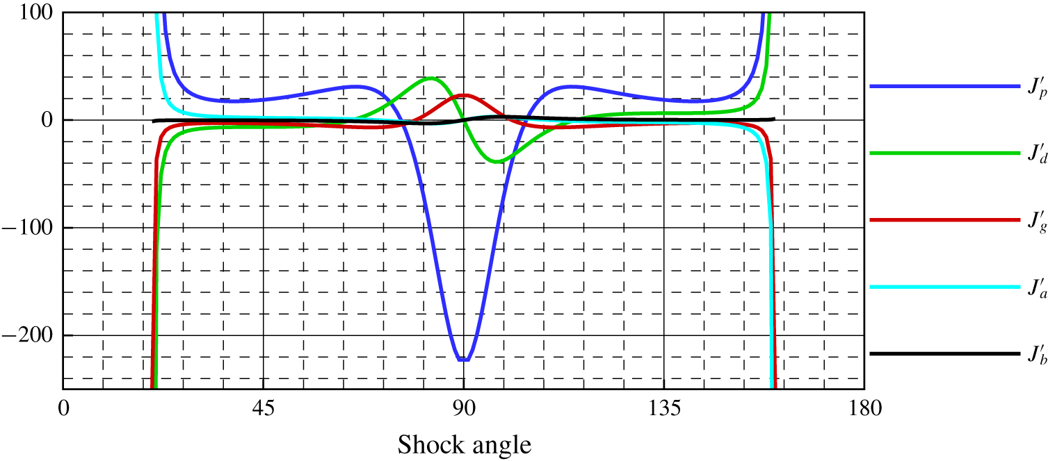
 $G^{\prime \prime \prime }$. In figure 3 we show the influence coefficients for the post-shock second-order pressure gradient
 $P_{2}^{\prime }$ for both an acute and an obtuse shock facing a Mach 3 air flow. The blue curve shows that, for weak shocks, the pre-shock second-order pressure gradient is amplified in the same sense by a factor of about 25, whereas, for strong shocks, the incoming gradient is amplified by as much as 200 with a reversal of sense. At some intermediate values of shock angle of about
 $76^{\circ }$ and
 $104^{\circ }$, the incoming second-order pressure gradient has no influence on the post-shock second-order gradient. The green curve shows that a pre-shock flow curvature gradient
 $D_{1}^{\prime }$ makes a negative contribution to the post-shock second-order pressure gradient for almost all acute weak shocks. The effect is antisymmetric for an obtuse shock. The contribution of the upstream vorticity gradient (red curve) to the post-shock second-order pressure gradient is in the opposite sense to that of the pre-shock second-order pressure gradient, but is otherwise similar. The contribution of the flow-plane curvature gradient
 $S_{a}^{\prime }$ to the second-order pressure gradient is shown by the cyan curve. The flow-plane curvature gradient has less effect on the post-shock second-order pressure gradient for most shock waves. The black curve shows the influence of the lateral shock curvature gradient
 $S_{b}^{\prime }$ on the post-shock second-order pressure gradient when there is no flow divergence/convergence in front of the shock. There can be, however, a change in divergence/convergence, as represented by
 $\unicode[STIX]{x2202}\unicode[STIX]{x1D6FF}_{1}/\unicode[STIX]{x2202}\unicode[STIX]{x1D70E}$, contributing to
 $S_{b}^{\prime }$.
Influence coefficients for the second-order pressure gradient.

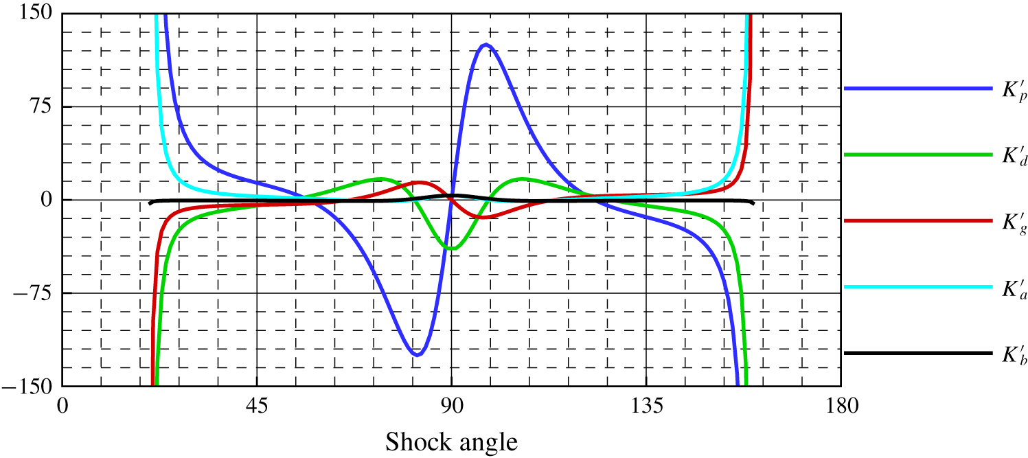
Influence coefficients for the streamline curvature gradient.

In figure 4 we depict the influence coefficients for the pre-shock and shock curvature gradient terms affecting the post-shock flow curvature gradient  $D_{2}^{\prime }$. The blue curve shows that a positive pre-shock second-order pressure gradient contributes positively to the post-shock curvature gradient for a weak acute shock and negatively for a strong acute shock. The effect is antisymmetric for an obtuse shock. The green curve shows that the pre-shock flow curvature gradient has no influence on the post-shock curvature gradient near acute shock angles of
 $53^{\circ }$ and
 $81^{\circ }$ and obtuse shock angles of
 $99^{\circ }$ and
 $127^{\circ }$. The contribution of the pre-shock vorticity gradient (red curve) is similar, except that there are only three shock angles at which there is no contribution. The cyan and black curves show the symmetric effects of the two shock curvature gradients
 $S_{a}^{\prime }$ and
 $S_{b}^{\prime }$.
The graphs in figures 3 and 4 are either symmetric or antisymmetric for acute and obtuse shocks. This is because the free stream has been set to be parallel to the axis of symmetry ( $\unicode[STIX]{x1D6FF}_{1}=0$). A non-zero value of
 $\unicode[STIX]{x1D6FF}_{1}$ has no effect in planar flow, but in axial flow, it leads to pre-shock flow convergence or divergence effects.
2.3.2 Variation of second-order parameters for planar shock waves
Next, the second-order curved shock equations, as derived above, are applied to planar shock waves and conical shocks. Again, because of the uniform and irrotational free stream, the left-hand sides of the second-order curved shock equations are zero. For planar shock waves, the transverse curvature  $S_{b}$ is also zero, as is the transverse curvature gradient
 $S_{b}^{\prime }$. However, the curvature in the flow plane has a finite value,
 $S_{a}\neq 0$ for planar curved shock waves and
 $S_{a}=0$ for planar linear shock waves, as well as the gradient of the shock curvature
 $S_{a}^{\prime }$. Under these conditions, the second-order curved shock equations become
 $$\begin{eqnarray}\displaystyle & \displaystyle P_{2}^{\prime }=J_{a}^{\prime }S_{a}^{\prime }+J_{pl}^{\prime }S_{a}^{2}, & \displaystyle\end{eqnarray}$$
 $$\begin{eqnarray}\displaystyle & \displaystyle D_{2}^{\prime }=K_{a}^{\prime }S_{a}^{\prime }+K_{pl}^{\prime }S_{a}^{2}, & \displaystyle\end{eqnarray}$$
where the coefficients  $J_{pl}^{\prime }$ and
 $K_{pl}^{\prime }$ are given in appendix B.
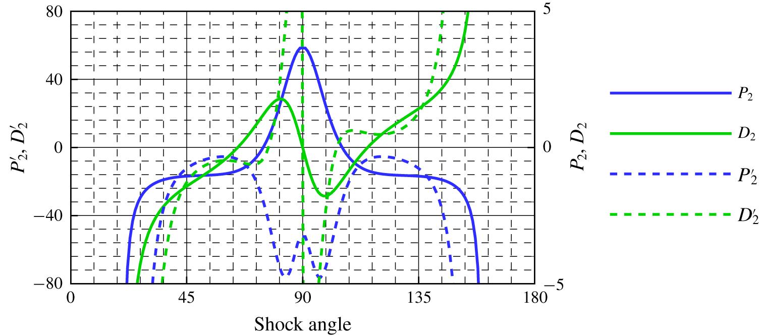
Second-order pressure gradient and flow curvature gradient behind a planar shock in uniform flow ( $Ma=3$ and
 $S_{a}=-1$).

Equations (2.33) and (2.34) state that, immediately behind the shock, the second-order pressure gradient along the streamline and the streamline curvature gradient are both quadratically dependent on the shock curvature  $S_{a}$. The magnitude and sign of the dependence are determined by the coefficients. These coefficients are functions of the free stream Mach number and the shock angle only. In figure 5 we plot
 $P_{2}^{\prime }$ and
 $D_{2}^{\prime }$ for a free stream Mach number of 3 and a convex shock with a curvature of
 $-1$ and
 $S_{a}^{\prime }=0$. At obtuse shock angles where
 $\unicode[STIX]{x1D703}>104^{\circ }$ and stronger acute shock angles where
 $\unicode[STIX]{x1D703}>77^{\circ }$, the flow curvature gradient (green dashed lines) is positive, while it is negative at other shock angles. The second-order pressure gradient (blue dashed lines) is negative for all shock angles. At the Thomas and Crocco points, where
 $P_{2}$ and
 $D_{2}$, respectively, are zero on the shock wave,
 $P_{2}^{\prime }$ and
 $D_{2}^{\prime }$ are no longer equal to zero. They are useful guideposts in the landscape of changing flow fields near curved shocks. The second-order theory can be regarded as a supplement to the Thomas and Crocco points. For instance, it is the Thomas point that separates compressive and expansive flow fields. With the information from
 $P_{2}^{\prime }$, the compressive and expansive strengths can be analysed. Furthermore, the parameter
 $P_{2}^{\prime }$ is the factor that determines whether the Thomas point can be continued along the streamline to become a Thomas streamline. It is the Crocco point that identifies the flow tendency. The rate of change of flow direction is determined by the variable
 $D_{2}^{\prime }$, and it is this variable that provides further information regarding whether a streamline is linear or curved.
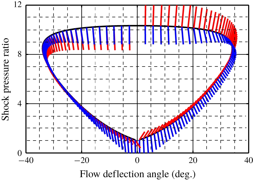
Shock polar and polar streamline behind a planar shock in uniform flow ( $Ma=3$ and
 $S_{a}=-1$).

2.3.3 Pressure/deflection polar for planar shock waves
Pressure and flow deflection are two important variables for shock reflections. Taking Mach reflection as an example, the pressure and flow direction remain the same on both sides of the slip layer, whereas the values of other parameters may change (von Neumann Reference von Neumann1943). This characteristic is the basis for the application of the pressure/deflection polar (Naca 1952). A typical pressure/deflection polar with associated streamline and its gradient is shown in figure 6. The vertical coordinate is the pressure ratio  $p$ and the horizontal coordinate is flow deflection
 $\unicode[STIX]{x1D6FF}$. If the shock is curved, then there is a value of
 $P_{2}^{\prime }$ and
 $D_{2}^{\prime }$ associated with every point on the shock polar, and the flow ‘direction’ gradient in the
 $(p,\unicode[STIX]{x1D6FF})$ plane can then be written as
 $$\begin{eqnarray}l_{pl}^{\prime }=\frac{{\displaystyle \frac{1}{\unicode[STIX]{x1D70C}V^{2}Ma_{1}^{2}}}{\displaystyle \frac{\unicode[STIX]{x2202}^{2}p}{\unicode[STIX]{x2202}s^{2}}}}{{\displaystyle \frac{\unicode[STIX]{x2202}\unicode[STIX]{x1D6FF}^{2}}{\unicode[STIX]{x2202}s^{2}}}}=\frac{1}{\unicode[STIX]{x1D70C}V^{2}Ma_{1}^{2}}\frac{\unicode[STIX]{x2202}^{2}p}{\unicode[STIX]{x2202}\unicode[STIX]{x1D6FF}^{2}}=\frac{P^{\prime }}{Ma_{1}^{2}D^{2}}=\frac{J_{pl}^{\prime }-J_{a}^{\prime }{\displaystyle \frac{\unicode[STIX]{x2202}R_{a}}{\unicode[STIX]{x2202}\unicode[STIX]{x1D70E}}}}{Ma_{1}^{2}K_{a}^{2}}.\end{eqnarray}$$
The black curve in figure 6 is the shock polar, the red lines show the slope of the ‘streamline’ behind the planar symmetric shock and the blue lines show the flow ‘direction’ gradient, here denoted by  $l_{pl}^{\prime }$. The right-hand side of the figure represents acute shocks, with positive flow deflection, and the left-hand side represents obtuse shocks, with negative flow deflection. For a weak acute shock,
 $l_{pl}^{\prime }$ is negative, opposite to the slope of the ‘streamline’. At the Crocco point (
 $\pm 34^{\circ }$), the slope goes through
 $\pm \infty$. So does the flow ‘direction’ gradient. At the Thomas point (
 $\pm 31^{\circ }$), the slope goes through another change of sign, but the flow ‘direction’ gradient still has the same sign as before. For acute shock angles, the slope and the flow ‘direction’ gradient are in opposite senses, while, for the obtuse shock, their senses are the same. In planar flow, the polar streamline slope is independent of shock curvature (Mölder Reference Mölder2015). However, the flow ‘direction’ gradient is related to the shock curvature. With this characteristic, the polar figure can be applied to the study of shock reflections. For regular reflection, the parameters behind the incident shock must match the variables before the reflected shock. Thus, not only must the incident post-shock
 $P/D$ be equal to the reflected pre-shock
 $P/D$, but also the values of
 $P^{\prime }/D^{2}$ must be the same in the regions behind the incident shock and before the reflected shock. A relation between the gradients of the incident shock curvature and the reflected shock curvature can then be constructed. As for the Mach reflection, owing to the von Neumann condition, the quantity
 $Ma^{2}P^{\prime }/D^{2}$ must remain the same across the slip layer. Thus, the curvatures of incident, reflected and Mach shocks are connected by the second-order curved shock equations.
2.3.4 Variation of second-order parameters for conical shock waves
When the flow is associated with a conical shock, curved shock theory can be utilized to develop the post-shock flow second-order gradient terms facing a uniform upstream flow, which means that  $P_{1}^{\prime }=D_{1}^{\prime }=\unicode[STIX]{x1D6E4}_{1}^{\prime }=0$,
 $S_{a}=0$ and
 $S_{b}=-1/R_{b}=-\cos \unicode[STIX]{x1D703}_{1}/y$. The free stream is parallel to the
 $x$ axis, so
 $\unicode[STIX]{x1D6FF}_{1}=0$, which makes
 $G^{\prime \prime }=0$. Then, the second-order curved shock equations become
 $$\begin{eqnarray}\displaystyle & \displaystyle P_{2}^{\prime }=J_{b}^{\prime }S_{b}^{\prime }+J_{cs}^{\prime }S_{b}^{2}, & \displaystyle\end{eqnarray}$$
 $$\begin{eqnarray}\displaystyle & \displaystyle D_{2}^{\prime }=K_{b}^{\prime }S_{b}^{\prime }+K_{cs}^{\prime }S_{b}^{2}, & \displaystyle\end{eqnarray}$$
where the coefficients  $J_{cs}^{\prime }$ and
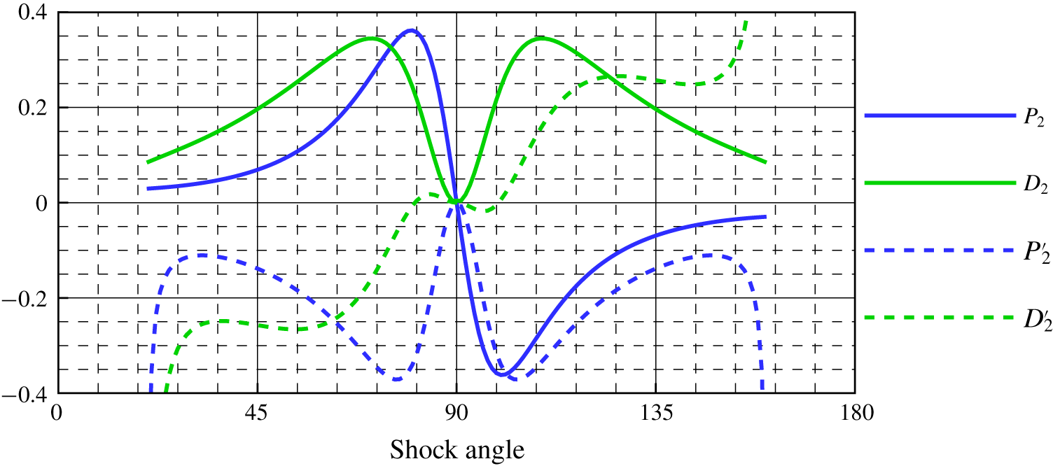
 $K_{cs}^{\prime }$ are given in appendix B. These second-order gradients are plotted in figure 7 for a Mach number of 3 and for streamlines that originate at a point on the shock that is located a unit distance from the centreline
 $y=1$. The left half of this figure is for a cone with an acute shock angle and the right half for an obtuse conical shock. For an acute conical shock, both
 $P_{2}^{\prime }$ and
 $D_{2}^{\prime }$ are negative, confirming that in the flow behind an acute conical shock the pressure increases more slowly along the streamline, as does the flow inclination. These are both conditions known to exist in flow over a circular cone at zero angle of attack. For the less familiar obtuse conical shock, the lateral streamline curvature gradient is positive, but the second-order pressure gradient is negative, so the pressure decreases more slowly, but the streamline inclination increases more rapidly along the streamline.
Second-order pressure gradient and flow curvature gradient behind a conical shock in uniform flow ( $Ma=3$ and
 $y=1$).

2.3.5 Pressure/deflection polar for conical shock waves
Using (2.36) and (2.37) for conical flow gives the polar streamline slope
 $$\begin{eqnarray}l_{cs}^{\prime }=\frac{{\displaystyle \frac{1}{\unicode[STIX]{x1D70C}V^{2}Ma_{1}^{2}}}{\displaystyle \frac{\unicode[STIX]{x2202}^{2}p}{\unicode[STIX]{x2202}s^{2}}}}{{\displaystyle \frac{\unicode[STIX]{x2202}\unicode[STIX]{x1D6FF}^{2}}{\unicode[STIX]{x2202}s^{2}}}}=\frac{1}{\unicode[STIX]{x1D70C}V^{2}Ma_{1}^{2}}\frac{\unicode[STIX]{x2202}^{2}p}{\unicode[STIX]{x2202}\unicode[STIX]{x1D6FF}^{2}}=\frac{P^{\prime }}{Ma_{1}^{2}D^{2}}=\frac{J_{cs}^{\prime }-J_{b}^{\prime }{\displaystyle \frac{\unicode[STIX]{x2202}R_{b}}{\unicode[STIX]{x2202}\unicode[STIX]{x1D70E}}}}{Ma_{1}^{2}K_{b}^{2}}.\end{eqnarray}$$
In figure 8 the red lines show the slopes of the ‘streamline’ for conical flow, while the blue lines are the flow ‘direction’ gradient, here denoted by  $l_{cs}^{\prime }$. These correspond to (2.35) for planar flow. An examination of the nature of
 $P_{2}^{\prime }$,
 $P_{2}$ and
 $D_{2}$ shows that the flow ‘direction’ gradient in the
 $(p,\unicode[STIX]{x1D6FF})$-plane is a function of the free stream Mach number, shock angle and shock curvature
 $S_{b}$. For most acute shock angles, the slope and the flow ‘direction’ gradient are in the opposite sense, except for part of the weak acute shock. In conical flow, the polar streamline slope is independent of shock curvature. However, the flow ‘direction’ gradient is related to shock curvature, as in planar flow. Unlike planar flow, however, there is no possibility of a Crocco or Thomas point on a conical shock, so the slope behind a conical shock is never zero. However, points where the ‘streamline’ curvature gradient is zero do exist. As in planar symmetric flow, the application of the second-order equations to the pressure/deflection polar facilitates the study of shock reflections in an axisymmetric flow field by establishing relations between the curvatures of incident, reflected and Mach shocks. Since the shock curvature is related to the shock geometry, the second-order curved shock equations provide a novel perspective from which to investigate aspects of shock reflections, such as the shape of the Mach disk.
Shock polar and polar streamline behind a conical shock in uniform flow ( $Ma=3$ and
 $y=1$).

3 Application of second-order curved shock theory to post-shock flow field calculation
The greatest restriction on curved shock theory is that it gives answers only in the close neighbourhood of shock waves. However,  $P_{2}^{\prime }$ and
 $D_{2}^{\prime }$ are two variables that could be used to approximately solve the post-shock flow field under some hypotheses. From their definitions, note that for a conical shock,
 $P_{2}^{\prime }$ and
 $D_{2}^{\prime }$ are functions of post-shock Mach number, shock angle and transverse curvature
 $S_{b}$. Thus, a selected conical flow field is calculated, and the parameters along the streamlines are evaluated with post-processing software. With these parameters,
 $P_{2}$,
 $D_{2}$,
 $P_{2}^{\prime }$ and
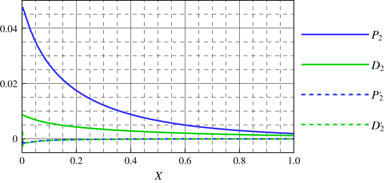
 $D_{2}^{\prime }$ can then be calculated along the streamline using the central difference method, and are plotted in figure 9. It can be seen that although
 $P_{2}$ (blue solid curve) and
 $D_{2}$ (red solid curve) change greatly along the streamline,
 $P_{2}^{\prime }$ (blue dashed curve) and
 $D_{2}^{\prime }$ (red dashed curve) barely change. Therefore, curved shock theory can also be used to approximately solve the flow field behind a curved shock under the assumption that
 $P_{2}$ and
 $D_{2}$ or
 $P_{2}^{\prime }$ and
 $D_{2}^{\prime }$ are constants along the streamline. According to the assumption, post-shock streamlines can be drawn as follows by using Taylor series at the shock wave:
 $$\begin{eqnarray}\displaystyle & \displaystyle y=y_{s}+(x-x_{s})\tan \unicode[STIX]{x1D6FF}+\frac{(x-x_{s})^{2}}{2}\frac{\text{d}^{2}y}{\text{d}x^{2}}+\frac{(x-x_{s})^{3}}{6}\frac{\text{d}^{3}y}{\text{d}x^{3}}+\cdots \,, & \displaystyle \nonumber\\ \displaystyle & \displaystyle \frac{\text{d}^{2}y}{\text{d}x^{2}}=\frac{D_{2}}{\cos ^{3}\unicode[STIX]{x1D6FF}},\quad \frac{\text{d}^{3}y}{\text{d}x^{3}}=\frac{3D_{2}^{2}\tan \unicode[STIX]{x1D6FF}+D_{2}^{\prime }}{\cos ^{4}\unicode[STIX]{x1D6FF}}. & \displaystyle \nonumber\end{eqnarray}$$
The post-shock flow field is then updated using the vorticity equation (2.5). Most interestingly, this is the case not only for an axisymmetric linear shock, but also for planar and axisymmetric curved shocks. To confirm the feasibility of the theory, the curved shock equations and the second-order equations are applied here to three typical curved shocks with uniform oncoming flow. For comparison, the method of characteristics is then also used to calculate the flow field. The characteristic equations and compatibility relations for the method of characteristics are as follows:
 $$\begin{eqnarray}\displaystyle & \displaystyle \left(\frac{\text{d}y}{\text{d}x}\right)_{0}=\frac{V_{y}}{V_{x}}, & \displaystyle \nonumber\\ \displaystyle & \displaystyle \left(\frac{\text{d}y}{\text{d}x}\right)_{\pm }=\tan \!\left[\unicode[STIX]{x1D6FF}_{2}\pm \arcsin \!\left(\frac{1}{Ma}\right)\right], & \displaystyle \nonumber\\ \displaystyle & \displaystyle \unicode[STIX]{x1D70C}V\,\text{d}_{0}V+\text{d}_{0}p=0, & \displaystyle \nonumber\\ \displaystyle & \displaystyle \text{d}_{0}p-V_{sonic}^{2}\,\text{d}_{0}\unicode[STIX]{x1D70C}=0, & \displaystyle \nonumber\\ \displaystyle & \displaystyle \text{d}_{\pm }\unicode[STIX]{x1D6FF}_{2}\pm \frac{(Ma^{2}-1)^{\frac{1}{2}}}{\unicode[STIX]{x1D70C}V^{2}}\,\text{d}_{\pm }p+\frac{j\sin \unicode[STIX]{x1D6FF}_{2}\,\text{d}_{\pm }x}{yMa\cos \!\left[\unicode[STIX]{x1D6FF}_{2}\pm \arcsin \!\left({\displaystyle \frac{1}{Ma}}\right)\right]}=0. & \displaystyle \nonumber\end{eqnarray}$$
We use the following notation:  $0$, streamline direction;
 $\pm$, characteristic direction; and
 $j$, planar flow
 $(j=0)$ or axially symmetric flow
 $(j=1)$.
Flow gradients along the streamline behind a conical shock in uniform flow ( $Ma=3$ and
 $\unicode[STIX]{x1D703}=30^{\circ }$).

3.1 Axisymmetric linear shock ( $S_{a}=0$, $S_{b}\neq 0$)


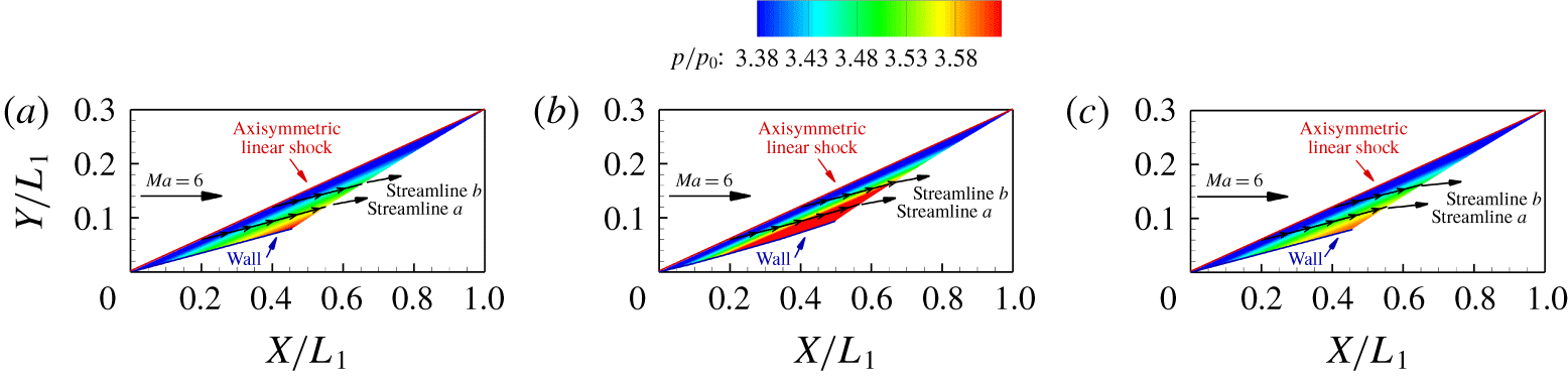
The flow character of the flow field behind an axisymmetric linear shock at incoming Mach number 6 is shown in figure 10. The shock wave has only one curvature and its shape is a frustum of a cone, like a conical shock wave with a centre body. The shock angle in the flow plane is  $16.7^{\circ }$. The reference length is
 $L_{1}=50$ for dimensionless treatment. The flow fields calculated using the method of characteristics, the curved shock equations and the second-order curved shock equations are separately represented in figure 10. All three post-shock flow fields have similar flow character. However, owing to a difference between the real and supposed values in the hypothesis that
 $P_{2}$ and
 $D_{2}$ are constants along the streamline, the pressure ratio given by the curved shock equations is larger than that given by the method of characteristics, especially in the region far from the shock. Increasing the order of the flow parameters gives a better match with the results of the method of characteristics, as can be seen from figure 10. The reason is that
 $P_{2}^{\prime }$ and
 $D_{2}^{\prime }$ remain almost constant along the streamlines compared with
 $P_{2}$ and
 $D_{2}$, and, as mentioned above, this increases the accuracy significantly.
Pressure flow field behind an axisymmetric linear shock  $y/L_{1}=0.3x/L_{1}$ (
 $S_{a}=0$,
 $S_{b}\neq 0$,
 $Ma=6$,
 $L_{1}=50$): (a) method of characteristics; (b) first-order curved shock equations; (c) second-order curved shock equations.

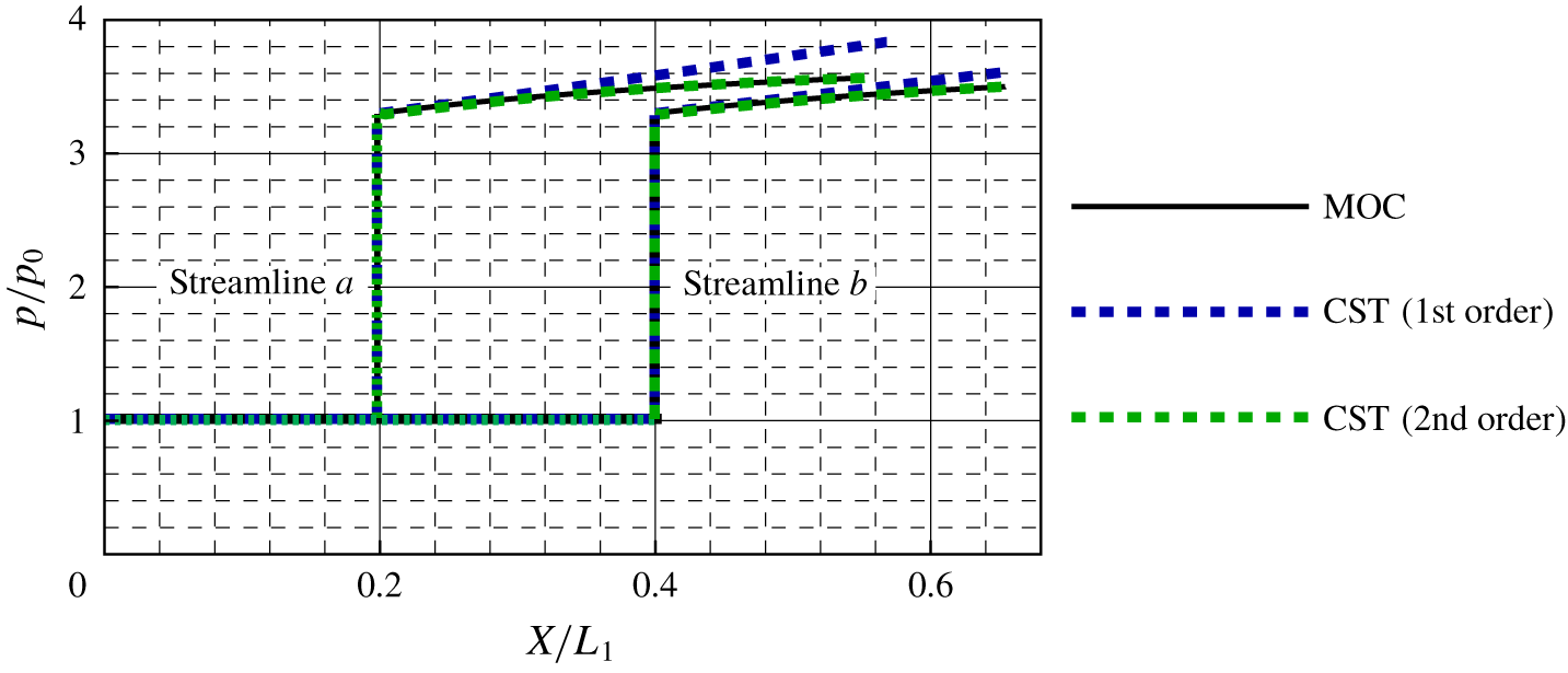
Pressure distribution along streamlines ( $S_{a}=0$ and
 $S_{b}\neq 0$) from the method of characteristics (MOC) and the first- and second-order curved shock equations (CST).

For a quantitative analysis, streamlines originating from the shock at  $x/L_{1}=0.2$ and 0.4 are extracted from the three flow fields as shown in figure 11. The blue curves show that, in comparison with the method of characteristics (the black curves), the difference in the pressure ratio calculated using the first-order curved shock equations increases along the streamlines and there is a huge gap at the end of the streamlines. Furthermore, as a streamline comes closer to the wall, the deviation becomes greater. The maximum deviation in the pressure ratio from the first-order curved shock equations along streamline ‘a’ occurs at the end, and is 6.8 %. However, on increasing the order of the curved shock equations, the accuracy improves significantly, as shown by the green curves for the second-order equations. This close coincidence between the green and black curves exists not only far from the wall, but also close to the wall, which demonstrates the accuracy of the second-order curved shock equations in obtaining the post-shock flow field. In comparison with the first-order curved shock equations, the maximum difference in the pressure ratio calculated using the second-order equations along streamline ‘a’ decreases significantly to 0.8 %.
3.2 Axisymmetric doubly curved shock ($S_{a}\neq 0$, $S_{b}\neq 0$)


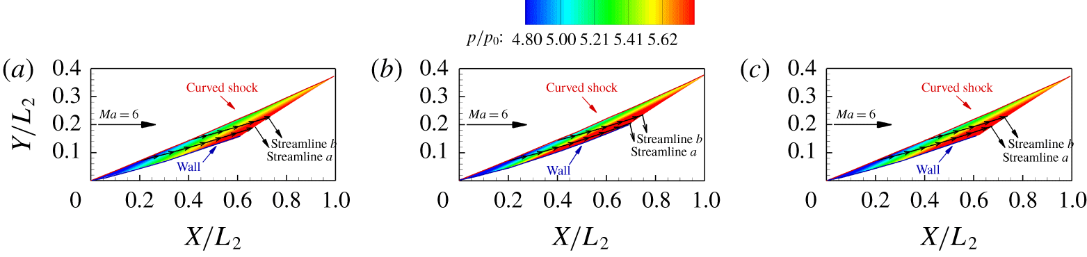
For an axisymmetric curved shock, the flow character of the post-shock flow fields at incoming Mach number 6 is shown in figure 12. The streamwise shape of the curved shock is a quadratic curve given by the equation  $y/L_{2}=0.025(x/L_{2})^{2}+0.35x/L_{2}$. The reference length is
 $L_{2}=50$ for dimensionless treatment. The cross-sectional geometry of the curved shock is circular, which means that the curvature of the shock wave in the flow-normal plane is non-zero. As shown in figure 12, three post-shock flow fields are computed by means of the method of characteristics, the first-order curved shock equations and the second-order curved shock equations, respectively. On the whole, the flow fields obtained using the first- and second-order curved shock equations have a flow character similar to that obtained using the method of characteristics. However, there are still differences. The pressure ratio from the first-order curved shock equations increases more rapidly than that from the method of characteristics. It can be seen from figure 12 that there is a better match between the results of the second-order curved shock equations and those of the method of characteristics.
Pressure flow field behind an axisymmetric curved shock  $y/L_{2}=0.025(x/L_{2})^{2}+0.35x/L_{2}$ (
 $S_{a}\neq 0$,
 $S_{b}\neq 0$,
 $Ma=6$ and
 $L_{2}=50$): (a) method of characteristics; (b) first-order curved shock equations; (c) second-order curved shock equations.

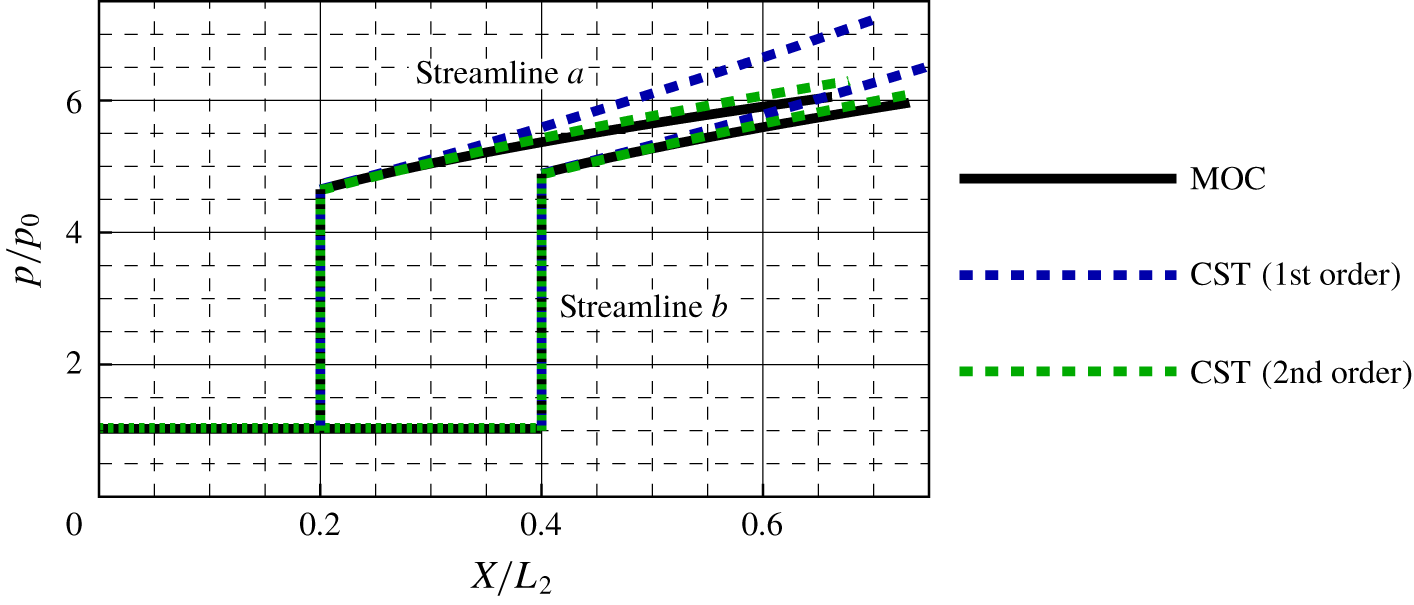
Pressure distribution along streamlines ( $S_{a}\neq 0$ and
 $S_{b}\neq 0$) from the method of characteristics and the first- and second-order curved shock equations.

The streamlines originating from the shock at  $x/L_{2}=0.2$ and 0.4 are extracted from the three flow fields for quantitative analysis. In figure 13 we show the pressure distribution along these streamlines. Compared with the method of characteristics (black curves), the deviation in the pressure ratio calculated using the first-order curved shock equations (blue curves) increases significantly along the streamline owing to the hypothesis that
 $P_{2}$ and
 $D_{2}$ are constants along the streamline. The maximum difference occurs at the end of streamline ‘a’, and is 19.8 %. In contrast, the results from the second-order curved shock equations (green curves) are close to those from the method of characteristics, which means that these equations could be used to solve the axisymmetric post-shock flow field with greater accuracy. It can be seen that the differences in the pressure ratio from the second-order curved shock equations increase downstream, but only slightly, with a maximum of 2.4 % at the end of streamline ‘a’. Thus, by increasing the order of the curved shock equations, the accuracy has significantly improved by 17.4 %.
3.3 Planar symmetric curved shock ($S_{a}\neq 0$, $S_{b}=0$)


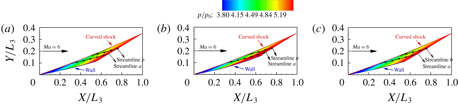
The equations are also used to approximately solve a planar post-shock flow field. In figure 14 we show the flow character of the flow fields behind a planar symmetric curved shock at incoming Mach number 6. The shock wave shape is a quadratic curve given by the equation  $y/L_{3}=0.05(x/L_{3})^{2}+0.3x/L_{3}$. The reference length is
 $L_{3}=100$ for dimensionless treatment. The results in figure 14 are acquired using the method of characteristics and the first- and second-order curved shock equations. All three post-shock flow fields show the same trend, with the pressure ratio increasing along the streamline. However, owing to the difference between the real and supposed values for
 $P_{2}$ and
 $D_{2}$ in the hypothesis that the pressure gradient and streamline curvature remain unchanged along the streamline, the pressure ratio from the first-order curved shock equations is greater than that from the method of characteristics, especially in the region far from the shock. From figure 14, it can be seen that there is a better coincidence between the results of the second-order curved shock equations and the method of characteristics, owing to the increasing order of the flow parameters. Compared with the method of characteristics, the difference in the pressure ratio from the first-order curved shock equations increases along the streamline. As the streamline comes closer to the wall, the deviation becomes larger, which is also the case for the flow field from the second-order curved shock equations. However, with the increased order of the curved shock equations, the maximum difference in pressure ratio is smaller.
Pressure flow field behind a planar symmetric curved shock  $y/L_{3}=0.05(x/L_{3})^{2}+0.3x/L_{3}$ (
 $S_{a}\neq 0$,
 $S_{b}=0$,
 $Ma=6$ and
 $L_{3}=100$): (a) method of characteristics; (b) first-order curved shock equations; (c) second-order curved shock equations.

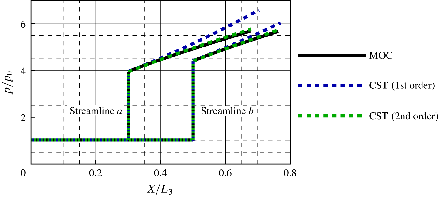
Pressure distribution along streamlines ( $S_{a}\neq 0$ and
 $S_{b}=0$) from the method of characteristics and the first- and second-order curved shock equations.

The pressure distribution for the three flow fields along streamlines originating from the shock at  $x/L_{3}=0.3$ and 0.5 is presented in figure 15. As before, the results of the method of characteristics, the first-order curved shock equations and the second-order curved shock equations are represented by black, blue and green curves, respectively. The pressure ratio calculated from the first-order curved shock equations (blue curves) again increases significantly along the streamlines, which leads to a large deviation from the result of the method of characteristics (black curves), with a maximum of 17.0 % at the end of streamline ‘a’. However, the results from the second-order curved shock equations (green curves) remain close to those of the method of characteristics, and the difference is controlled in a small range for the whole post-shock flow field, with a maximum of just 1.2 % at the end of streamline ‘a’. Thus, the second-order curved shock equations are capable also of calculating the planar post-shock flow field with good accuracy.
We have shown that the second-order curved shock equations are capable of calculating post-shock flow fields for planar and axisymmetric flow more accurately than the first-order curved shock equations. However, there are still differences with the results of the method of characteristics. The main reason for these is the assumption that  $P_{2}^{\prime }$ and
 $D_{2}^{\prime }$ are constants along the streamline. Although, from figure 9,
 $P_{2}^{\prime }$ and
 $D_{2}^{\prime }$ remain almost constant, there are still differences initially, as a result of which differences accumulate as the calculation proceeds. Furthermore, from (2.24) and (2.25), it can be seen that the curvature of the shock wave and the incoming flow parameters have effects on
 $P_{2}^{\prime }$ and
 $D_{2}^{\prime }$, which means that there are deviations depending on differences between shock waves and incoming flows. Fortunately, these differences are less than 5 % for most shock waves. Therefore, the second-order curved shock equations can be used for solving post-shock flow fields.
4 Application of curved shock theory to shock wave capture
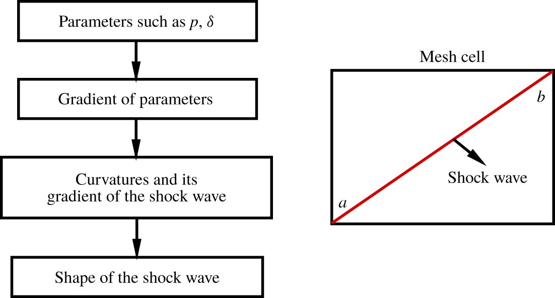
In addition to its use for post-shock flow field calculation, curved shock theory has another application to shock wave capture, owing to its advantage of high precision in the close neighbourhood of a shock wave. In the past, the Rankine–Hugoniot (R–H) equations were widely used for shock wave capture. However, the information acquired by the R–H equations is limited. Since high-order variables describing shock geometry can be acquired from the curved shock equations, curved shock theory is a better candidate for fitting the shock shape. In figure 16 we give the scheme of shock capture using curved shock theory. We consider a mesh cell as an example. The cell is shown by black lines and the shock wave is shown in red. Since the shock wave is divided into parts by the meshes, each part of the wave in a mesh cell can be considered as a curve. The mesh nodes through which the shock wave passes are then taken as endpoints of the shock wave. After the numerical simulation, information about aerodynamic parameters can be acquired at every mesh node, as can the gradients through high-order schemes. With information at the endpoints of the shock wave, the curvature of the shock wave and its gradient at points a and b can be solved with given pre-shock and post-shock parameters through the first- and second-order curved shock equations, respectively. The second derivative  $y^{\prime \prime }$ is then evaluated from the curvature of the shock wave via the equation
 $$\begin{eqnarray}S_{a}=\frac{y^{\prime \prime }}{(1+{y^{\prime }}^{2})^{3/2}},\end{eqnarray}$$
and the third derivative  $y^{\prime \prime \prime }$ is obtained from
 $$\begin{eqnarray}S_{a}^{\prime }=\frac{\text{d}S_{a}}{\text{d}\unicode[STIX]{x1D70E}}=\frac{y^{\prime \prime \prime }(1+{y^{\prime }}^{2})-3y^{\prime }{y^{\prime \prime }}^{2}}{(1+{y^{\prime }}^{2})^{3}}.\end{eqnarray}$$
With these derivatives, a high-order polynomial can be utilized to fit the shock curve. Two cases are presented here to verify this approach. The first case is a planar symmetric curved shock wave and the second is an axisymmetric doubly curved shock wave. Aerodynamic parameters and their gradients at the endpoints of a shock wave are input as given conditions. Both shock waves are fitted using three methods: the R–H equations, first-order curved shock theory and second-order curved shock theory.
Scheme of shock capture.

4.1 Planar symmetric curved shock ($S_{a}\neq 0$, $S_{b}=0$)


4.1.1 Shock capture with given aerodynamic parameters at the endpoints of a shock wave
In practical applications, only the pre- and post-shock parameters are needed to solve the shock wave geometry. However, for a quantitative analysis, a planar symmetric curved shock is given explicitly as a function  $y=\frac{1}{2}(\text{e}^{x}-1)$ with a range
 $0<x<1$. The post-shock parameters at the beginning and end of the shock curve are given at incoming Mach number 6. The pressure ratio is 8.2335 at the beginning of the shock curve and 27.0823 at the end. The given post-shock parameters are used to solve for the curvature of the shock wave and its gradient. The shock wave angles calculated from the R–H equations are then fitted with a linear equation
 $y^{\prime }=\tan \unicode[STIX]{x1D703}=0.8591x+0.5000$ using the least-squares method under the condition that parameters at the endpoints of the shock wave are known from computational fluid dynamics (CFD). Since the shock wave angle is connected to the slope of the shock wave, the shock wave is matched with a quadratic equation
 $y=0.4296x^{2}+0.5000x$, which is integrated from the equation
 $y^{\prime }=\tan \unicode[STIX]{x1D703}=0.8591x+0.5000$. Similarly, with the shock wave curvature
 $S_{a}$ evaluated from the first-order curved shock equations, the second derivative
 $y^{\prime \prime }$ can be obtained from (4.1). Afterwards, according to the least-squares method, the relation between the second derivative
 $y^{\prime \prime }$ and
 $x$ is fitted as
 $y^{\prime \prime }=0.8591x+0.5000$. Then, after two integrations, the shock wave is fitted as a cubic equation
 $y=0.1432x^{3}+0.2500x^{2}+0.4296x$. For second-order curved shock theory, the third derivative is evaluated from (4.2) and fitted as
 $y^{\prime \prime \prime }=0.8658x+0.5014$. After three integrations, the shock wave is fitted as a quartic equation
 $y=0.0361x^{4}+0.0836x^{3}+0.2124x^{2}+0.5393x$.
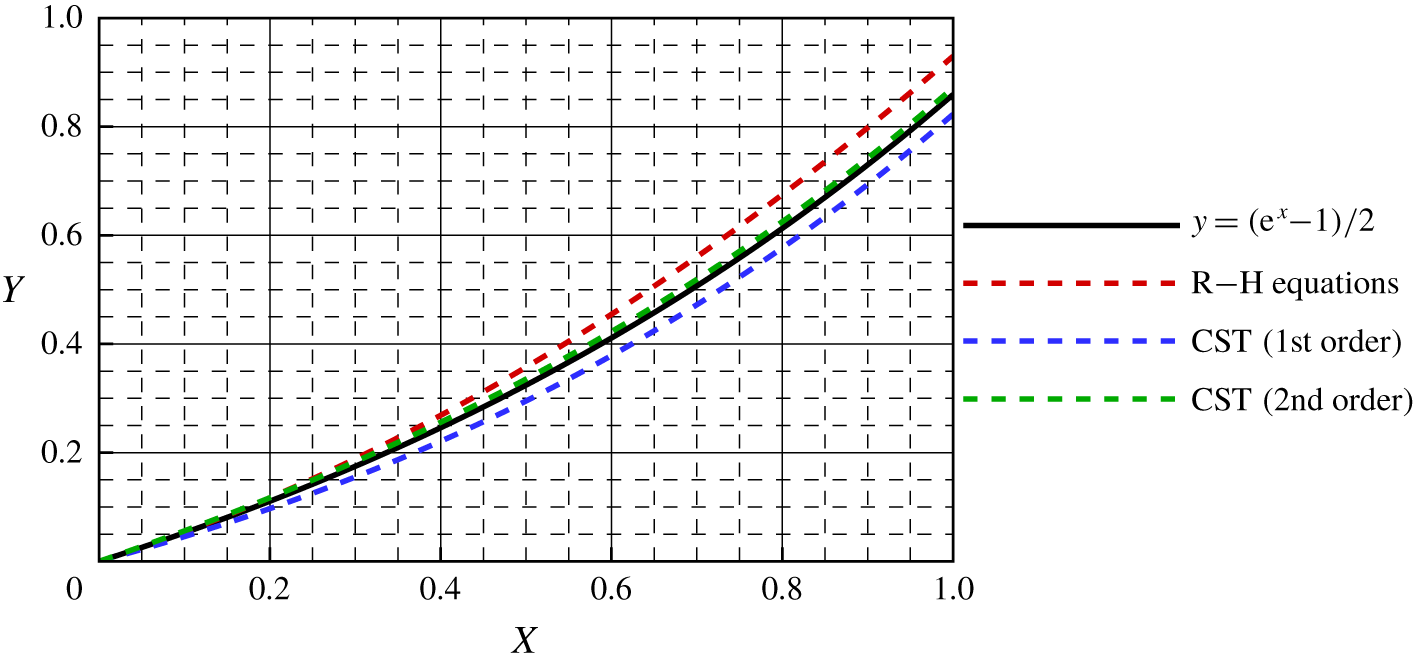
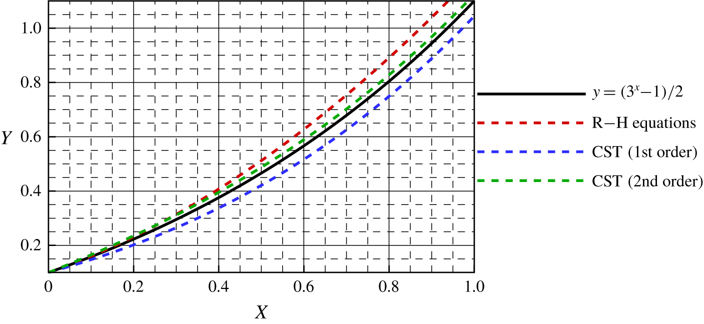
In figure 17 we show shock wave curves obtained by three different methods with given parameters of two mesh nodes at the shock wave. The original shock wave is represented by the black curve. The red, blue and green curves represent shock waves obtained using the R–H equations, first-order curved shock theory and second-order curved shock theory, respectively. From the comparison, it is clear that with the increase in order, the differences between the fitted and original curves decrease. The green curve is the closest to the black curve, whereas the red curve deviates the most, which demonstrates the merits of second-order curved shock theory in solving the geometry of shock waves.
Planar symmetric curved shocks solved by three methods with parameters of two mesh nodes given ( $S_{a}\neq 0$,
 $S_{b}=0$ and
 $Ma=6$).

Regression analysis for a planar symmetric curved shock with parameters of two mesh nodes given.

The results of a regression analysis are shown in table 1. The residual sum of squares (RSS) is a variable indicating the degree of fit of an equation to data. It is the sum of the squares of the deviations between equation values and data. The total sum of squares is defined as the sum of the squared differences of the dependent variable and its mean. Furthermore, goodness of fit  $R^{2}$ is a statistical model describing the extent of fit between fitted and original curves and ranges from 0 to 1. A large
 $R^{2}$ indicates a tight fit. From table 1, it can be seen that the maximum difference decreases from 0.0704 to 0.0364 when the method is changed from the R–H equations to first-order curved shock theory, and it decreases further to 0.0122 with the use of second-order curved shock theory. The RSS for the R–H equations is 0.1786, which is approximately three times as large as that for first-order curved shock theory. Furthermore, the RSS declines significantly when the second-order curved shock theory is used, which means that the accuracy is further improved. The
 $R^{2}$ value rises from 0.9714 to 0.9877 when the method is changed from the R–H equations to first-order curved shock theory and then to 0.9984 for second-order curved shock theory, which confirms that the fitted curve is similar to the original curve. However, it cannot be denied that a deviation still exists with only two mesh nodes given.
4.1.2 Shock capture with given aerodynamic parameters at the endpoints and midpoint of a shock wave
The parameters of three nodes at a shock wave are given from CFD as known conditions, at the endpoints and the midpoint of the shock wave. To ensure a fair comparison, shock angles calculated by the R–H equations are again matched with the linear equation using the least-squares method. Thus, based on the relation between angles and slopes of a shock wave, the shock wave is fitted with a quadratic equation  $y=0.4296x^{2}+0.4649x$, which is integrated from the equation
 $y^{\prime }=\tan \unicode[STIX]{x1D703}=0.8591x+0.4649$. Furthermore, since the shock wave curvature is related to the second derivative
 $y^{\prime \prime }$, the shock wave from the first-order curved shock theory is fitted as a cubic equation
 $y=0.1432x^{3}+0.2325x^{2}+0.4845x$ after two integrations. For the second-order curved shock theory, the shock wave is fitted as a quartic equation
 $y=0.0361x^{4}+0.0776x^{3}+0.2417x^{2}+0.5064x$ after three integrations.
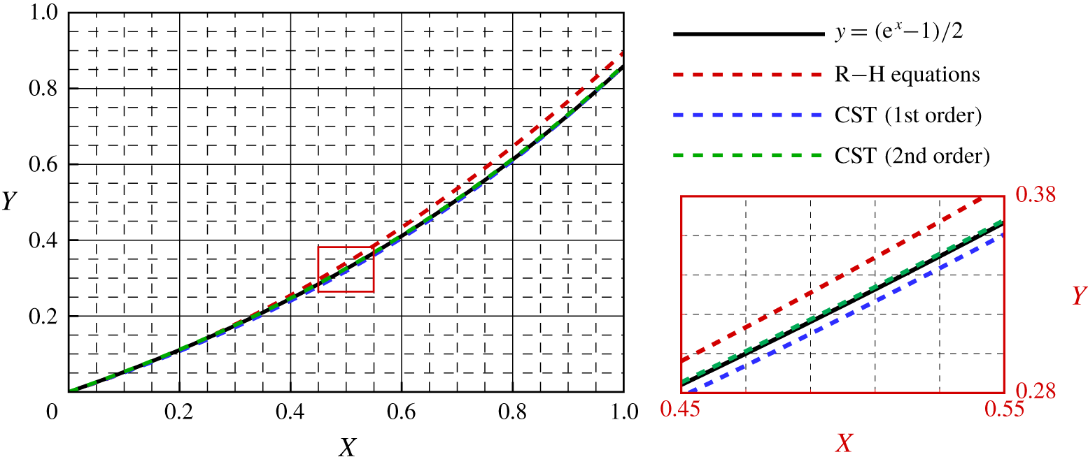
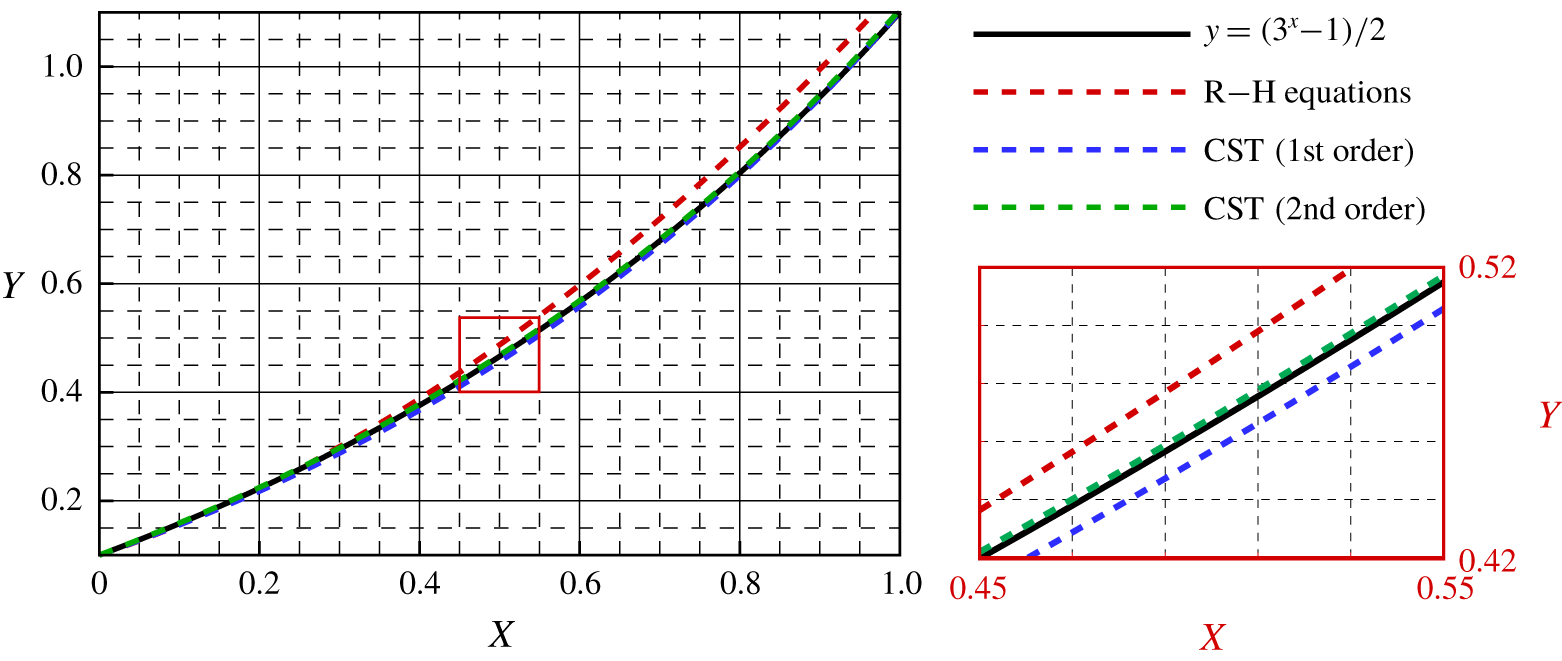
The fitted curves are plotted with different colours in figure 18: the original shock wave is shown by the black solid curve, while the red, blue and green dashed curves represent the shock waves obtained from the R–H equations, first-order curved shock theory and second-order curved shock theory, respectively. The section between 0.45 and 0.55 is magnified in the insert to show the curves more clearly. It can be seen that the fitted curve gets closer to the original curve as the order of the theory is increased. Even in the magnified area, the green curve for second-order curved shock theory is still almost the same as the original curve. In contrast, although the red and blue curves show a similar trend to the black curve, there are obvious differences.
Planar symmetric curved shock solved by three methods with parameters of three mesh nodes given ( $S_{a}\neq 0$,
 $S_{b}=0$ and
 $Ma=6$).

The results of a regression analysis for a planar symmetric curved shock with given parameters of three nodes at a shock wave are presented in table 2. It can be seen that the maximum difference for the R–H equations is 0.0367, and this goes down to 0.0061 for first-order curved shock theory. The maximum difference for second-order curved shock theory is the least, with a value of just 0.0026. The RSS for the R–H equations is 0.0489, which is approximately 25 times larger than for first-order curved shock theory. There is a significant further improvement in accuracy when the order of the theory is increased, and the RSS is decreased by an order of magnitude, to 0.0002, for second-order curved shock theory. The goodness of fit increases from 0.9922 to 0.9997 when first-order curved shock theory replaces the R–H equations, and this goes up to 1.0000 when second-order curved shock theory is used to fit the geometry of a given shock wave, which means that the fitted curve shows a good match with the original curve. In other words, the accuracy increases for all three methods when more parameters are given, and, furthermore, second-order curved shock theory yields solving the planar symmetric curved shock explicitly with only three mesh nodes given as known conditions.
4.2 Axisymmetric curved shock ($S_{a}\neq 0$, $S_{b}\neq 0$)


4.2.1 Shock capture with given aerodynamic parameters at the endpoints of a shock wave
Similarly to the first case, the geometry of the axisymmetric curved shock is in this case specified as an exponential curve given by the equation  $y=\frac{1}{2}(3^{x}-1)$ with
 $0<x<1$, and the height at the centre is 0.1. The oncoming Mach number is 6, and the parameters behind the shock wave are calculated by the method of characteristics. Only the parameters at the shock wave endpoints are given as known information. The linear equation
 $y^{\prime }=\tan \unicode[STIX]{x1D703}=1.0986x+0.5493$ is solved by the least-squares method to fit the shock wave angles. After the process of integration, the shock wave is fitted with the quadratic equation
 $y=0.5493x^{2}+0.5493x+0.1$. Accordingly, with the shock wave curvature
 $S_{a}$, the shock wave is matched as a cubic equation
 $y=0.2012x^{3}+0.3017x^{2}+0.4410x+0.1$ using the first-order shock wave equations. For second-order curved shock theory, the shock wave is fitted as a quartic equation
 $y=0.0567x^{4}+0.1110x^{3}+0.2318x^{2}+0.6243x+0.1$.
Regression analysis for a planar symmetric curved shock with parameters of three mesh nodes given.

Shock wave curves obtained by the three methods are presented in figure 19. As before, the black solid curve represents the original shock wave, and the red, blue and green dashed curves represent the shock waves calculated using the R–H equations, first-order curved shock theory and second-order curved shock theory, respectively. It is clear that the fitted curve is closer to the original curve when the order of the theory is increased, with the deviation between the green and black curves being least and the red curve showing the greatest deviation from the original. Thus, second-order curved shock theory again has the highest accuracy among the three methods.
Axisymmetric curved shock solved by three methods with parameters of two mesh nodes given ( $S_{a}\neq 0$ and
 $S_{b}\neq 0$).

In table 3 we present the results of a regression analysis for an axisymmetric curved shock with given parameters of two mesh nodes at a shock wave. First, the maximum difference for the R–H equations is 0.0986, which is about twice that for first-order curved shock theory, while second-order curved shock theory gives the lowest value, 0.0239, among the three methods. Second, the RSS for the R–H equations is 0.3485, which is approximately twice that for first-order curved shock theory. There is a further significant increase in accuracy for the second-order theory, with the RSS being an order of magnitude smaller, 0.0383. Finally, the goodness of fit rises from  $R^{2}=0.9587$ for the R–H equations to 0.9784 for first-order curved shock theory and to 0.9955 for the second-order theory. Thus, the shock curve from second-order curved shock theory agree fairly well with the original shock curve, although there is still a noticeable deviation when only information at the endpoints is given.
Regression analysis for an axisymmetric curved shock with parameters of two mesh nodes given.

4.2.2 Shock capture with given aerodynamic parameters at the endpoints and midpoint of a shock wave
To get a better fit, the number of known conditions is increased to three: at the endpoints and midpoint of the shock wave. As before, a linear equation solved by the least-squares method is applied to fit the shock wave angles:  $y^{\prime }=\tan \unicode[STIX]{x1D703}=1.0986x+0.5002$. The shock wave is then fitted with a quadratic equation
 $y=0.5493x^{2}+0.5002x+0.1$ after integration. Similarly, the shock wave is matched as a cubic equation
 $y=0.2012x^{3}+0.2748x^{2}+0.5258x+0.1$ by first-order curved shock theory and as a quartic equation
 $y=0.0567x^{4}+0.1003x^{3}+0.2871x^{2}+0.5608x+0.1$ by second-order curved shock theory.
All these expressions are plotted in figure 20. The region from 0.45 to 0.55 is magnified in the insert to give a clearer view of the curves. It can be seen that the fitted curves are closer to the original curve when more conditions are given. However, there is still an obvious difference between the red and black curves representing the results of the R–H equations and the original shock, respectively. The blue and green curves representing the results of first- and second-order curved shock theory show better agreement with the black curve. However, in the magnified area, it is clear that the deviation between the green and black curves is the least, whereas there is a greater, but still small, deviation between the blue and black curves. Thus, second-order curved shock theory again has an advantage over the other two methods for shock wave calculation.
Axisymmetric curved shock solved by three methods with parameters of three mesh nodes given ( $S_{a}\neq 0$ and
 $S_{b}\neq 0$).

In table 4 we present the results of a regression analysis for the axisymmetric curved shock with given parameters of three mesh nodes at a shock wave. It can be seen that the maximum difference decreases significantly when information at an additional node is given. The value for the R–H equations is now 0.0514, which is still the greatest among the three methods. The maximum differences for first- and second-order curved shock theory are 0.0093 and 0.0049, respectively, about one-fifth of the values for the previous case. The RSS for the R–H equations is 0.0953, which is approximately one-third of the previous value. However, it is still much larger than the RSS for first-order curved shock theory, which in turn is an order of magnitude greater than that for second-order curved shock theory, 0.0006. Finally,  $R^{2}$, which describes the goodness of fit between the fitted and original curves, increases from 0.9887 for the R–H equations to 0.9995 for first-order curved shock theory and to 0.9999 for second-order curved shock theory, indicating that the fitted shock curve agrees well with the original curve. To sum up, second-order curved shock theory is again able to calculate the axisymmetric curved shock explicitly with the parameters of three nodes given.
Regression analysis for an axisymmetric curved shock with parameters of three mesh nodes given.

5 Conclusions
Second-order curved shock theory relates shock curvature gradients and flow divergence/convergence to the second-order gradients of pressure, vorticity and streamline curvature. In this paper, explicit expressions for the second-order flow gradients have been obtained in influence coefficient form. The first- and second-order curved shock equations have been applied to solve the post-shock flow field in both planar and axial flows. The results show that the second-order curved shock equations improve the accuracy of results by more than 10 % in comparison with the first-order curved shock equations. Curved shock theory has also been used to fit shock waves in planar and axisymmetric flows. Regression analyses show that the shock wave residual sum of squares for the second-order equations is an order of magnitude lower than those for the R–H and first-order equations. Furthermore, the goodness of fit for the second-order curved shock equations is almost 1 in both planar and axisymmetric flows, which means that the second-order curved shock equations can capture planar symmetric and axisymmetric shock waves explicitly with a limited number of given conditions, owing to the merits of using high-order variables. These high-order variables used to describe the shock geometry make this theory a good candidate for solving shock capture problems in CFD algorithms.
Acknowledgements
We would like to acknowledge the support of the National Natural Science Foundation of China (NSFC, grant no. 91941103) and Aeronautical Science Foundation of China (ASFC, grant no. 2018ZB68008).
Declaration of interests
The authors report no conflict of interest.
Appendix A. Derivation of second-order curved shock equations
Taking derivatives of both sides of each of (2.2) and (2.3) with respect to  $n$ (distance normal to the streamline) and
 $s$ (distance along the streamline), respectively, gives
 $$\begin{eqnarray}\displaystyle \left.\begin{array}{@{}c@{}}\displaystyle \frac{\unicode[STIX]{x2202}\unicode[STIX]{x1D70C}_{1}V_{1}^{2}P_{1}}{\unicode[STIX]{x2202}n}=-\frac{\unicode[STIX]{x2202}\unicode[STIX]{x1D70C}_{1}V_{1}^{2}D_{1}}{\unicode[STIX]{x2202}s},\\ \displaystyle \unicode[STIX]{x1D70C}_{1}V_{1}^{2}\frac{\unicode[STIX]{x2202}P_{1}}{\unicode[STIX]{x2202}n}+2V_{1}\unicode[STIX]{x1D70C}_{1}P_{1}\frac{\unicode[STIX]{x2202}V_{1}}{\unicode[STIX]{x2202}n}+V_{1}^{2}P_{1}\frac{\unicode[STIX]{x2202}\unicode[STIX]{x1D70C}_{1}}{\unicode[STIX]{x2202}n}=-\unicode[STIX]{x1D70C}_{1}V_{1}^{2}\frac{\unicode[STIX]{x2202}D_{1}}{\unicode[STIX]{x2202}s}-2V_{1}\unicode[STIX]{x1D70C}_{1}D_{1}\frac{\unicode[STIX]{x2202}V_{1}}{\unicode[STIX]{x2202}s}-V_{1}^{2}D_{1}\frac{\unicode[STIX]{x2202}\unicode[STIX]{x1D70C}_{1}}{\unicode[STIX]{x2202}s}.\end{array}\right\} & & \displaystyle \nonumber\\ \displaystyle & & \displaystyle\end{eqnarray}$$
The derivatives  $\unicode[STIX]{x2202}\bullet /\unicode[STIX]{x2202}s$ and
 $\unicode[STIX]{x2202}\bullet /\unicode[STIX]{x2202}n$ can be expressed in the following forms:
 $$\begin{eqnarray}\displaystyle \frac{\unicode[STIX]{x2202}V_{k}}{\unicode[STIX]{x2202}s}=-P_{k}V_{k},\quad \frac{\unicode[STIX]{x2202}V_{k}}{\unicode[STIX]{x2202}n}=V_{k}(D_{k}-\unicode[STIX]{x1D6E4}_{k}), & & \displaystyle \nonumber\\ \displaystyle \frac{\unicode[STIX]{x2202}\unicode[STIX]{x1D70C}_{k}}{\unicode[STIX]{x2202}s}=\unicode[STIX]{x1D70C}_{k}Ma_{k}^{2}P_{k},\quad \frac{\unicode[STIX]{x2202}\unicode[STIX]{x1D70C}_{k}}{\unicode[STIX]{x2202}n}=-\unicode[STIX]{x1D70C}_{k}Ma_{k}^{2}[D_{k}+(\unicode[STIX]{x1D6FE}-1)\unicode[STIX]{x1D6E4}_{k}]. & & \displaystyle \nonumber\end{eqnarray}$$
Here  $k=1,2$ depending on whether the application is to flow before or after the shock. With these substitutions, (A 1) becomes
 $$\begin{eqnarray}\displaystyle & & \displaystyle \unicode[STIX]{x1D70C}_{1}V_{1}^{2}\frac{\unicode[STIX]{x2202}P_{1}}{\unicode[STIX]{x2202}n}+2\unicode[STIX]{x1D70C}_{1}V_{1}^{2}P_{1}(D_{1}-\unicode[STIX]{x1D6E4}_{1})-\unicode[STIX]{x1D70C}_{1}V_{1}^{2}P_{1}Ma_{1}^{2}[D_{1}+(\unicode[STIX]{x1D6FE}-1)\unicode[STIX]{x1D6E4}_{1}]\nonumber\\ \displaystyle & & \displaystyle \qquad =-\unicode[STIX]{x1D70C}_{1}V_{1}^{2}\frac{\unicode[STIX]{x2202}D_{1}}{\unicode[STIX]{x2202}s}+2\unicode[STIX]{x1D70C}_{1}V_{1}^{2}D_{1}P_{1}-\unicode[STIX]{x1D70C}_{1}V_{1}^{2}Ma_{1}^{2}P_{1}D_{1}.\end{eqnarray}$$
On replacing  $\unicode[STIX]{x2202}D_{1}/\unicode[STIX]{x2202}s$ by
 $D_{1}^{\prime }$, (A 2) becomes
 $$\begin{eqnarray}\frac{\unicode[STIX]{x2202}P_{1}}{\unicode[STIX]{x2202}n}=-D_{1}^{\prime }+(\unicode[STIX]{x1D6FE}-1)P_{1}Ma_{1}^{2}\unicode[STIX]{x1D6E4}_{1}+2P_{1}\unicode[STIX]{x1D6E4}_{1}.\end{eqnarray}$$
Similarly, for subscript 2, the following equation is obtained:
 $$\begin{eqnarray}\frac{\unicode[STIX]{x2202}P_{2}}{\unicode[STIX]{x2202}n}=-D_{2}^{\prime }+(\unicode[STIX]{x1D6FE}-1)P_{2}Ma_{2}^{2}\unicode[STIX]{x1D6E4}_{2}+2P_{2}\unicode[STIX]{x1D6E4}_{2}.\end{eqnarray}$$
Taking derivatives of both sides of each of (2.1) and (2.3) with respect to  $s$ and
 $n$, respectively, gives
 $$\begin{eqnarray}\left.\begin{array}{@{}c@{}}\displaystyle -\frac{\unicode[STIX]{x2202}\left[(Ma_{1}^{2}-1)P_{1}+{\displaystyle \frac{\sin \unicode[STIX]{x1D6FF}_{1}}{y_{1}}}\right]}{\unicode[STIX]{x2202}s}=\frac{\unicode[STIX]{x2202}D_{1}}{\unicode[STIX]{x2202}n},\\ \displaystyle \frac{\unicode[STIX]{x2202}D_{1}}{\unicode[STIX]{x2202}n}=-P_{1}\frac{\unicode[STIX]{x2202}Ma_{1}^{2}}{\unicode[STIX]{x2202}s}-(Ma_{1}^{2}-1)\frac{\unicode[STIX]{x2202}P_{1}}{\unicode[STIX]{x2202}s}-\frac{y_{1}\cos \unicode[STIX]{x1D6FF}_{1}{\displaystyle \frac{\unicode[STIX]{x2202}\unicode[STIX]{x1D6FF}_{1}}{\unicode[STIX]{x2202}s}}-\sin ^{2}\unicode[STIX]{x1D6FF}_{1}}{y_{1}^{2}}.\end{array}\right\}\end{eqnarray}$$
On replacing  $\unicode[STIX]{x2202}P_{1}/\unicode[STIX]{x2202}s$ by
 $P_{1s}^{\prime }$, (A 3) becomes
 $$\begin{eqnarray}\frac{\unicode[STIX]{x2202}D_{1}}{\unicode[STIX]{x2202}n}=-P_{1}\frac{\unicode[STIX]{x2202}Ma_{1}^{2}}{\unicode[STIX]{x2202}s}-(Ma_{1}^{2}-1)P_{1s}^{\prime }-\frac{\cos \unicode[STIX]{x1D6FF}_{1}\,D_{1}}{y_{1}}+\frac{\sin ^{2}\unicode[STIX]{x1D6FF}_{1}}{y_{1}^{2}}.\end{eqnarray}$$
Similarly, for subscript 2, the following equation is obtained:
 $$\begin{eqnarray}\frac{\unicode[STIX]{x2202}D_{2}}{\unicode[STIX]{x2202}n}=-P_{2}\frac{\unicode[STIX]{x2202}Ma_{2}^{2}}{\unicode[STIX]{x2202}s}-(Ma_{2}^{2}-1)P_{2s}^{\prime }-\frac{\cos \unicode[STIX]{x1D6FF}_{2}\,D_{2}}{y_{2}}+\frac{\sin ^{2}\unicode[STIX]{x1D6FF}_{2}}{y_{2}^{2}}.\end{eqnarray}$$
Derivation of the second-order curved shock equations (2.20) and (2.21) starts from (2.8) and (2.9),
 $$\begin{eqnarray}A_{1}^{\ast }P_{1}+B_{1}^{\ast }D_{1}+E_{1}^{\ast }\unicode[STIX]{x1D6E4}_{1}=A_{2}^{\ast }P_{2}+B_{2}^{\ast }D_{2}+C^{\ast }S_{a}+G^{\ast }S_{b}.\end{eqnarray}$$
The superscript  $\ast$ is used to identify the equations. For instance,
 $A_{1}^{\ast }$ equals to
 $A_{1}$ for (2.20) and represents
 $A_{1}^{\prime }$ for (2.21). Taking derivatives of both sides with respect to
 $\unicode[STIX]{x1D70E}$ gives
 $$\begin{eqnarray}\displaystyle & & \displaystyle A_{1}^{\ast }\frac{\unicode[STIX]{x2202}P_{1}}{\unicode[STIX]{x2202}\unicode[STIX]{x1D70E}}+P_{1}\frac{\unicode[STIX]{x2202}A_{1}^{\ast }}{\unicode[STIX]{x2202}\unicode[STIX]{x1D70E}}+B_{1}^{\ast }\frac{\unicode[STIX]{x2202}D_{1}}{\unicode[STIX]{x2202}\unicode[STIX]{x1D70E}}+D_{1}\frac{\unicode[STIX]{x2202}B_{1}^{\ast }}{\unicode[STIX]{x2202}\unicode[STIX]{x1D70E}}+E_{1}^{\ast }\frac{\unicode[STIX]{x2202}\unicode[STIX]{x1D6E4}_{1}}{\unicode[STIX]{x2202}\unicode[STIX]{x1D70E}}+\unicode[STIX]{x1D6E4}_{1}\frac{\unicode[STIX]{x2202}E_{1}^{\ast }}{\unicode[STIX]{x2202}\unicode[STIX]{x1D70E}}\nonumber\\ \displaystyle & & \displaystyle \qquad =A_{2}^{\ast }\frac{\unicode[STIX]{x2202}P_{2}}{\unicode[STIX]{x2202}\unicode[STIX]{x1D70E}}+P_{2}\frac{\unicode[STIX]{x2202}A_{2}^{\ast }}{\unicode[STIX]{x2202}\unicode[STIX]{x1D70E}}+B_{2}^{\ast }\frac{\unicode[STIX]{x2202}D_{2}}{\unicode[STIX]{x2202}\unicode[STIX]{x1D70E}}+D_{2}\frac{\unicode[STIX]{x2202}B_{2}^{\ast }}{\unicode[STIX]{x2202}\unicode[STIX]{x1D70E}}+C^{\ast }\frac{\unicode[STIX]{x2202}S_{a}}{\unicode[STIX]{x2202}\unicode[STIX]{x1D70E}}+S_{a}\frac{\unicode[STIX]{x2202}C^{\ast }}{\unicode[STIX]{x2202}\unicode[STIX]{x1D70E}}+G^{\ast }\frac{\unicode[STIX]{x2202}S_{b}}{\unicode[STIX]{x2202}\unicode[STIX]{x1D70E}}+S_{b}\frac{\unicode[STIX]{x2202}G^{\ast }}{\unicode[STIX]{x2202}\unicode[STIX]{x1D70E}}.\nonumber\end{eqnarray}$$
Changing  $\unicode[STIX]{x1D70E}$-derivatives to
 $s$- and
 $n$-derivatives gives
 $$\begin{eqnarray}\displaystyle & & \displaystyle A_{1}^{\ast }\left(\frac{\unicode[STIX]{x2202}P_{1}}{\unicode[STIX]{x2202}s}\cos \unicode[STIX]{x1D703}+\frac{\unicode[STIX]{x2202}P_{1}}{\unicode[STIX]{x2202}n}\sin \unicode[STIX]{x1D703}\right)+P_{1}\frac{\unicode[STIX]{x2202}A_{1}^{\ast }}{\unicode[STIX]{x2202}\unicode[STIX]{x1D70E}}+B_{1}^{\ast }\left(\frac{\unicode[STIX]{x2202}D_{1}}{\unicode[STIX]{x2202}s}\cos \unicode[STIX]{x1D703}+\frac{\unicode[STIX]{x2202}D_{1}}{\unicode[STIX]{x2202}n}\sin \unicode[STIX]{x1D703}\right)\nonumber\\ \displaystyle & & \displaystyle \qquad +\,D_{1}\frac{\unicode[STIX]{x2202}B_{1}^{\ast }}{\unicode[STIX]{x2202}\unicode[STIX]{x1D70E}}+E_{1}^{\ast }\frac{\unicode[STIX]{x2202}\unicode[STIX]{x1D6E4}_{1}}{\unicode[STIX]{x2202}\unicode[STIX]{x1D70E}}+\unicode[STIX]{x1D6E4}_{1}\frac{\unicode[STIX]{x2202}E_{1}^{\ast }}{\unicode[STIX]{x2202}\unicode[STIX]{x1D70E}}\nonumber\\ \displaystyle & & \displaystyle \quad =A_{2}^{\ast }\left[\frac{\unicode[STIX]{x2202}P_{2}}{\unicode[STIX]{x2202}s}\cos (\unicode[STIX]{x1D703}-\unicode[STIX]{x1D6FF})+\frac{\unicode[STIX]{x2202}P_{2}}{\unicode[STIX]{x2202}n}\sin (\unicode[STIX]{x1D703}-\unicode[STIX]{x1D6FF})\right]+P_{2}\frac{\unicode[STIX]{x2202}A_{2}^{\ast }}{\unicode[STIX]{x2202}\unicode[STIX]{x1D70E}}\nonumber\\ \displaystyle & & \displaystyle \qquad +\,B_{2}^{\ast }\left[\frac{\unicode[STIX]{x2202}D_{2}}{\unicode[STIX]{x2202}s}\cos (\unicode[STIX]{x1D703}-\unicode[STIX]{x1D6FF})+\frac{\unicode[STIX]{x2202}D_{2}}{\unicode[STIX]{x2202}n}\sin (\unicode[STIX]{x1D703}-\unicode[STIX]{x1D6FF})\right]\nonumber\\ \displaystyle & & \displaystyle \qquad +\,D_{2}\frac{\unicode[STIX]{x2202}B_{2}^{\ast }}{\unicode[STIX]{x2202}\unicode[STIX]{x1D70E}}+C^{\ast }\frac{\unicode[STIX]{x2202}S_{a}}{\unicode[STIX]{x2202}\unicode[STIX]{x1D70E}}+S_{a}\frac{\unicode[STIX]{x2202}C^{\ast }}{\unicode[STIX]{x2202}\unicode[STIX]{x1D70E}}+G^{\ast }\frac{\unicode[STIX]{x2202}S_{b}}{\unicode[STIX]{x2202}\unicode[STIX]{x1D70E}}+S_{b}\frac{\unicode[STIX]{x2202}G^{\ast }}{\unicode[STIX]{x2202}\unicode[STIX]{x1D70E}}.\nonumber\end{eqnarray}$$
With some substitutions, this equation becomes
 $$\begin{eqnarray}\displaystyle & & \displaystyle A_{1}^{\ast }P_{1s}^{\prime }\cos \unicode[STIX]{x1D703}+P_{1}\frac{\unicode[STIX]{x2202}A_{1}^{\ast }}{\unicode[STIX]{x2202}\unicode[STIX]{x1D70E}}+B_{1}^{\ast }D_{1}^{\prime }\cos \unicode[STIX]{x1D703}+A_{1}^{\ast }\sin \unicode[STIX]{x1D703}\left[-D_{1}^{\prime }+\left(\unicode[STIX]{x1D6FE}-1\right)P_{1}Ma_{1}^{2}\unicode[STIX]{x1D6E4}_{1}+2P_{1}\unicode[STIX]{x1D6E4}_{1}\right]\nonumber\\ \displaystyle & & \displaystyle \qquad +\,B_{1}^{\ast }\sin \unicode[STIX]{x1D703}\left[-P_{1}\frac{\unicode[STIX]{x2202}Ma_{1}^{2}}{\unicode[STIX]{x2202}s}-\left(M_{1}^{2}-1\right)P_{1s}^{\prime }-\frac{\cos \unicode[STIX]{x1D6FF}_{1}D_{1}}{y_{1}}+\frac{\sin ^{2}\unicode[STIX]{x1D6FF}_{1}}{y_{1}^{2}}\right]\nonumber\\ \displaystyle & & \displaystyle \qquad +\,D_{1}\frac{\unicode[STIX]{x2202}B_{1}^{\ast }}{\unicode[STIX]{x2202}\unicode[STIX]{x1D70E}}+E_{1}^{\ast }\frac{\unicode[STIX]{x2202}\unicode[STIX]{x1D6E4}_{1}}{\unicode[STIX]{x2202}\unicode[STIX]{x1D70E}}+\unicode[STIX]{x1D6E4}_{1}\frac{\unicode[STIX]{x2202}E_{1}^{\ast }}{\unicode[STIX]{x2202}\unicode[STIX]{x1D70E}}\nonumber\\ \displaystyle & & \displaystyle \quad =A_{2}^{\ast }P_{2s}^{\prime }\cos (\unicode[STIX]{x1D703}-\unicode[STIX]{x1D6FF})+P_{2}\frac{\unicode[STIX]{x2202}A_{2}^{\ast }}{\unicode[STIX]{x2202}\unicode[STIX]{x1D70E}}+A_{2}^{\ast }\sin (\unicode[STIX]{x1D703}-\unicode[STIX]{x1D6FF})\left[-D_{2}^{\prime }+\left(\unicode[STIX]{x1D6FE}-1\right)P_{2}Ma_{2}^{2}\unicode[STIX]{x1D6E4}_{2}+2P_{2}\unicode[STIX]{x1D6E4}_{2}\right]\nonumber\\ \displaystyle & & \displaystyle \qquad +\,B_{2}^{\ast }D_{2}^{\prime }\cos (\unicode[STIX]{x1D703}-\unicode[STIX]{x1D6FF})+B_{2}^{\ast }\sin (\unicode[STIX]{x1D703}-\unicode[STIX]{x1D6FF})\nonumber\\ \displaystyle & & \displaystyle \qquad \times \,\left[-P_{2}\frac{\unicode[STIX]{x2202}Ma_{2}^{2}}{\unicode[STIX]{x2202}s}-(Ma_{2}^{2}-1)P_{2s}^{\prime }-\frac{\cos \unicode[STIX]{x1D6FF}_{2}D_{2}}{y_{2}}+\frac{\sin ^{2}\unicode[STIX]{x1D6FF}_{2}}{y_{2}^{2}}\right]\nonumber\\ \displaystyle & & \displaystyle \qquad +\,D_{2}\frac{\unicode[STIX]{x2202}B_{2}^{\ast }}{\unicode[STIX]{x2202}\unicode[STIX]{x1D70E}}+C^{\ast }\frac{\unicode[STIX]{x2202}S_{a}}{\unicode[STIX]{x2202}\unicode[STIX]{x1D70E}}+S_{a}\frac{\unicode[STIX]{x2202}C^{\ast }}{\unicode[STIX]{x2202}\unicode[STIX]{x1D70E}}+G^{\ast }\frac{\unicode[STIX]{x2202}S_{b}}{\unicode[STIX]{x2202}\unicode[STIX]{x1D70E}}+S_{b}\frac{\unicode[STIX]{x2202}G^{\ast }}{\unicode[STIX]{x2202}\unicode[STIX]{x1D70E}}.\end{eqnarray}$$
On replacing  $1/y$ by
 $-S_{b}/\text{cos}\,\unicode[STIX]{x1D703}_{1}$, (A 4) becomes
 $$\begin{eqnarray}\displaystyle & & \displaystyle A_{1}^{\ast }P_{1s}^{\prime }\cos \unicode[STIX]{x1D703}+P_{1}\frac{\unicode[STIX]{x2202}A_{1}^{\ast }}{\unicode[STIX]{x2202}\unicode[STIX]{x1D70E}}+B_{1}^{\ast }D_{1}^{\prime }\cos \unicode[STIX]{x1D703}+A_{1}^{\ast }\sin \unicode[STIX]{x1D703}\left[-D_{1}^{\prime }+\left(\unicode[STIX]{x1D6FE}-1\right)P_{1}Ma_{1}^{2}\unicode[STIX]{x1D6E4}_{1}+2P_{1}\unicode[STIX]{x1D6E4}_{1}\right]\nonumber\\ \displaystyle & & \displaystyle \qquad +\,B_{1}^{\ast }\sin \unicode[STIX]{x1D703}\left[-P_{1}\frac{\unicode[STIX]{x2202}Ma_{1}^{2}}{\unicode[STIX]{x2202}s}-(Ma_{1}^{2}-1)P_{1s}^{\prime }+\frac{S_{b}\cos \unicode[STIX]{x1D6FF}_{1}D_{1}}{\cos \unicode[STIX]{x1D703}_{1}}+\left(\frac{S_{b}\sin \unicode[STIX]{x1D6FF}_{1}}{\cos \unicode[STIX]{x1D703}_{1}}\right)^{2}\right]\nonumber\\ \displaystyle & & \displaystyle \qquad +\,D_{1}\frac{\unicode[STIX]{x2202}B_{1}^{\ast }}{\unicode[STIX]{x2202}\unicode[STIX]{x1D70E}}+E_{1}^{\ast }\frac{\unicode[STIX]{x2202}\unicode[STIX]{x1D6E4}_{1}}{\unicode[STIX]{x2202}\unicode[STIX]{x1D70E}}+\unicode[STIX]{x1D6E4}_{1}\frac{\unicode[STIX]{x2202}E_{1}^{\ast }}{\unicode[STIX]{x2202}\unicode[STIX]{x1D70E}}\nonumber\\ \displaystyle & & \displaystyle \quad =A_{2}^{\ast }P_{2s}^{\prime }\cos (\unicode[STIX]{x1D703}-\unicode[STIX]{x1D6FF})+P_{2}\frac{\unicode[STIX]{x2202}A_{2}^{\ast }}{\unicode[STIX]{x2202}\unicode[STIX]{x1D70E}}+B_{2}^{\ast }D_{2}^{\prime }\cos (\unicode[STIX]{x1D703}-\unicode[STIX]{x1D6FF})\nonumber\\ \displaystyle & & \displaystyle \qquad +\,A_{2}^{\ast }\sin (\unicode[STIX]{x1D703}-\unicode[STIX]{x1D6FF})\left[-D_{2}^{\prime }+\left(\unicode[STIX]{x1D6FE}-1\right)P_{2}Ma_{2}^{2}\unicode[STIX]{x1D6E4}_{2}+2P_{2}\unicode[STIX]{x1D6E4}_{2}\right]\nonumber\\ \displaystyle & & \displaystyle \qquad +\,B_{2}^{\ast }\sin (\unicode[STIX]{x1D703}-\unicode[STIX]{x1D6FF})\left[-P_{2}\frac{\unicode[STIX]{x2202}Ma_{2}^{2}}{\unicode[STIX]{x2202}s}-(Ma_{2}^{2}-1)P_{2s}^{\prime }+\frac{S_{b}\cos \unicode[STIX]{x1D6FF}_{2}D_{2}}{\cos \unicode[STIX]{x1D703}_{1}}+\left(\frac{S_{b}\sin \unicode[STIX]{x1D6FF}_{2}}{\cos \unicode[STIX]{x1D703}_{1}}\right)^{2}\right]\nonumber\\ \displaystyle & & \displaystyle \qquad +\,D_{2}\frac{\unicode[STIX]{x2202}B_{2}^{\ast }}{\unicode[STIX]{x2202}\unicode[STIX]{x1D70E}}+C^{\ast }\frac{\unicode[STIX]{x2202}S_{a}}{\unicode[STIX]{x2202}\unicode[STIX]{x1D70E}}+S_{a}\frac{\unicode[STIX]{x2202}C^{\ast }}{\unicode[STIX]{x2202}\unicode[STIX]{x1D70E}}+G^{\ast }\frac{\unicode[STIX]{x2202}S_{b}}{\unicode[STIX]{x2202}\unicode[STIX]{x1D70E}}+S_{b}\frac{\unicode[STIX]{x2202}G^{\ast }}{\unicode[STIX]{x2202}\unicode[STIX]{x1D70E}}.\nonumber\end{eqnarray}$$
Collecting terms gives
 $$\begin{eqnarray}\displaystyle & & \displaystyle \left[A_{1}^{\ast }\cos \unicode[STIX]{x1D703}-B_{1}^{\ast }\sin \unicode[STIX]{x1D703}(Ma_{1}^{2}-1)\right]P_{1}^{\prime }+\left[-\sin \unicode[STIX]{x1D703}A_{1}^{\ast }+B_{1}^{\ast }\cos \unicode[STIX]{x1D703}\right]D_{1}^{\prime }+E_{1}^{\ast }\frac{\unicode[STIX]{x2202}\unicode[STIX]{x1D6E4}_{1}}{\unicode[STIX]{x2202}\unicode[STIX]{x1D70E}}\nonumber\\ \displaystyle & & \displaystyle \quad =\left[A_{2}^{\ast }\cos (\unicode[STIX]{x1D703}-\unicode[STIX]{x1D6FF})-B_{2}^{\ast }(Ma_{2}^{2}-1)\sin (\unicode[STIX]{x1D703}-\unicode[STIX]{x1D6FF})\right]P_{2}^{\prime }\nonumber\\ \displaystyle & & \displaystyle \qquad +\,\left[-A_{2}^{\ast }\sin (\unicode[STIX]{x1D703}-\unicode[STIX]{x1D6FF})+B_{2}^{\ast }\cos (\unicode[STIX]{x1D703}-\unicode[STIX]{x1D6FF})\right]D_{2}^{\prime }\nonumber\\ \displaystyle & & \displaystyle \qquad +\,C^{\ast }\frac{\unicode[STIX]{x2202}S_{a}}{\unicode[STIX]{x2202}\unicode[STIX]{x1D70E}}+G^{\ast }\frac{\unicode[STIX]{x2202}S_{b}}{\unicode[STIX]{x2202}\unicode[STIX]{x1D70E}}\nonumber\\ \displaystyle & & \displaystyle \qquad +\,A_{2}^{\ast }P_{2}\left[\left(\left(\unicode[STIX]{x1D6FE}-1\right)Ma_{2}^{2}+2\right)\unicode[STIX]{x1D6E4}_{2}\sin (\unicode[STIX]{x1D703}-\unicode[STIX]{x1D6FF})\right.\left.+\cos (\unicode[STIX]{x1D703}-\unicode[STIX]{x1D6FF})P_{2}\left(2-Ma_{2}^{2}\right)\right]\nonumber\\ \displaystyle & & \displaystyle \qquad +\,B_{2}^{\ast }\sin (\unicode[STIX]{x1D703}-\unicode[STIX]{x1D6FF})\left[(Ma_{2}^{2}-1)P_{2}^{2}\left(Ma_{2}^{2}-2\right)-P_{2}\frac{\unicode[STIX]{x2202}Ma_{2}^{2}}{\unicode[STIX]{x2202}s}\right.\nonumber\\ \displaystyle & & \displaystyle \qquad \left.+\,\frac{S_{b}\cos \unicode[STIX]{x1D6FF}_{2}D_{2}}{\cos \unicode[STIX]{x1D703}_{1}}+\left(\frac{S_{b}\sin \unicode[STIX]{x1D6FF}_{2}}{\cos \unicode[STIX]{x1D703}_{1}}\right)^{2}\right]\nonumber\\ \displaystyle & & \displaystyle \qquad -\,A_{1}^{\ast }P_{1}\left[\left(\left(\unicode[STIX]{x1D6FE}-1\right)Ma_{1}^{2}+2\right)\unicode[STIX]{x1D6E4}_{1}\sin \unicode[STIX]{x1D703}+\cos \unicode[STIX]{x1D703}P_{1}\left(2-Ma_{1}^{2}\right)\right]\nonumber\\ \displaystyle & & \displaystyle \qquad -\,B_{1}^{\ast }\sin \unicode[STIX]{x1D703}\left[(Ma_{1}^{2}-1)P_{1}^{2}\left(Ma_{1}^{2}-2\right)-P_{1}\frac{\unicode[STIX]{x2202}Ma_{1}^{2}}{\unicode[STIX]{x2202}s}\right.\left.+\frac{S_{b}\cos \unicode[STIX]{x1D6FF}_{1}D_{1}}{\cos \unicode[STIX]{x1D703}_{1}}+\left(\frac{S_{b}\sin \unicode[STIX]{x1D6FF}_{1}}{\cos \unicode[STIX]{x1D703}_{1}}\right)^{2}\right]\nonumber\\ \displaystyle & & \displaystyle \qquad -\,P_{1}\frac{\unicode[STIX]{x2202}A_{1}^{\ast }}{\unicode[STIX]{x2202}\unicode[STIX]{x1D70E}}-D_{1}\frac{\unicode[STIX]{x2202}B_{1}^{\ast }}{\unicode[STIX]{x2202}\unicode[STIX]{x1D70E}}-\unicode[STIX]{x1D6E4}_{1}\frac{\unicode[STIX]{x2202}E_{1}^{\ast }}{\unicode[STIX]{x2202}\unicode[STIX]{x1D70E}}+P_{2}\frac{\unicode[STIX]{x2202}A_{2}^{\prime }}{\unicode[STIX]{x2202}\unicode[STIX]{x1D70E}}+D_{2}\frac{\unicode[STIX]{x2202}B_{2}^{\ast }}{\unicode[STIX]{x2202}\unicode[STIX]{x1D70E}}+S_{a}\frac{\unicode[STIX]{x2202}C^{\ast }}{\unicode[STIX]{x2202}\unicode[STIX]{x1D70E}}+S_{b}\frac{\unicode[STIX]{x2202}G^{\ast }}{\unicode[STIX]{x2202}\unicode[STIX]{x1D70E}},\nonumber\end{eqnarray}$$
where the unknown derivatives are given by
 $$\begin{eqnarray}\displaystyle & \displaystyle \frac{\unicode[STIX]{x2202}A_{2}}{\unicode[STIX]{x2202}\unicode[STIX]{x1D70E}}=\frac{\unicode[STIX]{x2202}{\displaystyle \frac{\sin \unicode[STIX]{x1D703}\cos \unicode[STIX]{x1D703}}{\sin (\unicode[STIX]{x1D703}-\unicode[STIX]{x1D6FF})}}}{\unicode[STIX]{x2202}\unicode[STIX]{x1D70E}}=\frac{\sin (\unicode[STIX]{x1D703}-\unicode[STIX]{x1D6FF})\cos 2\unicode[STIX]{x1D703}{\displaystyle \frac{\unicode[STIX]{x2202}\unicode[STIX]{x1D703}}{\unicode[STIX]{x2202}\unicode[STIX]{x1D70E}}}-\sin \unicode[STIX]{x1D703}\cos \unicode[STIX]{x1D703}\cos (\unicode[STIX]{x1D703}-\unicode[STIX]{x1D6FF}){\displaystyle \frac{\unicode[STIX]{x2202}(\unicode[STIX]{x1D703}-\unicode[STIX]{x1D6FF})}{\unicode[STIX]{x2202}\unicode[STIX]{x1D70E}}}}{\sin ^{2}(\unicode[STIX]{x1D703}-\unicode[STIX]{x1D6FF})}, & \displaystyle \nonumber\\ \displaystyle & \displaystyle \frac{\unicode[STIX]{x2202}B_{2}}{\unicode[STIX]{x2202}\unicode[STIX]{x1D70E}}=-\frac{\unicode[STIX]{x2202}{\displaystyle \frac{\sin \unicode[STIX]{x1D703}\cos \unicode[STIX]{x1D703}}{\cos (\unicode[STIX]{x1D703}-\unicode[STIX]{x1D6FF})}}}{\unicode[STIX]{x2202}\unicode[STIX]{x1D70E}}=-\frac{\cos (\unicode[STIX]{x1D703}-\unicode[STIX]{x1D6FF})\cos 2\unicode[STIX]{x1D703}{\displaystyle \frac{\unicode[STIX]{x2202}\unicode[STIX]{x1D703}}{\unicode[STIX]{x2202}\unicode[STIX]{x1D70E}}}+\sin \unicode[STIX]{x1D703}\cos \unicode[STIX]{x1D703}\sin (\unicode[STIX]{x1D703}-\unicode[STIX]{x1D6FF}){\displaystyle \frac{\unicode[STIX]{x2202}(\unicode[STIX]{x1D703}-\unicode[STIX]{x1D6FF})}{\unicode[STIX]{x2202}\unicode[STIX]{x1D70E}}}}{\cos ^{2}(\unicode[STIX]{x1D703}-\unicode[STIX]{x1D6FF})}, & \displaystyle \nonumber\\ \displaystyle & \displaystyle \frac{\unicode[STIX]{x2202}C}{\unicode[STIX]{x2202}\unicode[STIX]{x1D70E}}=-\frac{4}{\unicode[STIX]{x1D6FE}+1}\cos 2\unicode[STIX]{x1D703}{\displaystyle \frac{\unicode[STIX]{x2202}\unicode[STIX]{x1D703}}{\unicode[STIX]{x2202}\unicode[STIX]{x1D70E}}}, & \displaystyle \nonumber\end{eqnarray}$$

 $$\begin{eqnarray}\displaystyle & \displaystyle {\displaystyle \frac{\unicode[STIX]{x2202}B_{2}^{\prime }}{\unicode[STIX]{x2202}\unicode[STIX]{x1D70E}}}=-{\displaystyle \frac{\unicode[STIX]{x2202}\sin 2\unicode[STIX]{x1D703}}{\unicode[STIX]{x2202}\unicode[STIX]{x1D70E}}}=-2\cos 2\unicode[STIX]{x1D703}{\displaystyle \frac{\unicode[STIX]{x2202}\unicode[STIX]{x1D703}}{\unicode[STIX]{x2202}\unicode[STIX]{x1D70E}}}, & \displaystyle \nonumber\\ \displaystyle & \displaystyle {\displaystyle \frac{\unicode[STIX]{x2202}C^{\prime }}{\unicode[STIX]{x2202}\unicode[STIX]{x1D70E}}}=-{\displaystyle \frac{\unicode[STIX]{x2202}{\displaystyle \frac{\sin \left(2\unicode[STIX]{x1D6FF}\right)}{2\cos (\unicode[STIX]{x1D703}-\unicode[STIX]{x1D6FF})}}}{\unicode[STIX]{x2202}\unicode[STIX]{x1D70E}}}=-{\displaystyle \frac{4\cos (\unicode[STIX]{x1D703}-\unicode[STIX]{x1D6FF})\cos 2\unicode[STIX]{x1D6FF}{\displaystyle \frac{\unicode[STIX]{x2202}\unicode[STIX]{x1D6FF}}{\unicode[STIX]{x2202}\unicode[STIX]{x1D70E}}}+2\sin 2\unicode[STIX]{x1D6FF}\sin (\unicode[STIX]{x1D703}-\unicode[STIX]{x1D6FF}){\displaystyle \frac{\unicode[STIX]{x2202}(\unicode[STIX]{x1D703}-\unicode[STIX]{x1D6FF})}{\unicode[STIX]{x2202}\unicode[STIX]{x1D70E}}}}{4\cos ^{2}(\unicode[STIX]{x1D703}-\unicode[STIX]{x1D6FF})}}, & \displaystyle \nonumber\end{eqnarray}$$
 $$\begin{eqnarray}\displaystyle {\displaystyle \frac{\unicode[STIX]{x2202}A_{1}^{\prime }}{\unicode[STIX]{x2202}\unicode[STIX]{x1D70E}}} & = & \displaystyle {\displaystyle \frac{\unicode[STIX]{x2202}\left[Ma_{1}^{2}\cos ^{2}\unicode[STIX]{x1D703}\cos \unicode[STIX]{x1D6FF}-(Ma_{1}^{2}-1)\cos \left(2\unicode[STIX]{x1D703}+\unicode[STIX]{x1D6FF}\right)\right]}{\unicode[STIX]{x2202}\unicode[STIX]{x1D70E}}}\nonumber\\ \displaystyle & = & \displaystyle -2\sin \unicode[STIX]{x1D703}\cos \unicode[STIX]{x1D703}Ma_{1}^{2}\cos \unicode[STIX]{x1D6FF}{\displaystyle \frac{\unicode[STIX]{x2202}\unicode[STIX]{x1D703}}{\unicode[STIX]{x2202}\unicode[STIX]{x1D70E}}}-\sin \unicode[STIX]{x1D6FF}Ma_{1}^{2}\cos ^{2}\unicode[STIX]{x1D703}{\displaystyle \frac{\unicode[STIX]{x2202}\unicode[STIX]{x1D6FF}}{\unicode[STIX]{x2202}\unicode[STIX]{x1D70E}}}\nonumber\\ \displaystyle & & \displaystyle +\,\left[\cos \unicode[STIX]{x1D6FF}\cos ^{2}\unicode[STIX]{x1D703}-\cos \left(2\unicode[STIX]{x1D703}+\unicode[STIX]{x1D6FF}\right)\right]{\displaystyle \frac{\unicode[STIX]{x2202}Ma_{1}^{2}}{\unicode[STIX]{x2202}\unicode[STIX]{x1D70E}}}+\sin \left(2\unicode[STIX]{x1D703}+\unicode[STIX]{x1D6FF}\right)(Ma_{1}^{2}-1){\displaystyle \frac{\unicode[STIX]{x2202}\left(2\unicode[STIX]{x1D703}+\unicode[STIX]{x1D6FF}\right)}{\unicode[STIX]{x2202}\unicode[STIX]{x1D70E}}},\nonumber\end{eqnarray}$$

 $$\begin{eqnarray}\displaystyle \frac{\unicode[STIX]{x2202}Ma_{2}^{2}}{\unicode[STIX]{x2202}s} & = & \displaystyle \frac{1}{\unicode[STIX]{x1D6FE}p_{2}}\left(-2\unicode[STIX]{x1D70C}_{2}V_{2}^{2}P_{2}+Ma_{2}^{2}\unicode[STIX]{x1D70C}_{2}V_{2}^{2}P_{2}\right)-\frac{\unicode[STIX]{x1D70C}_{2}^{2}V_{2}^{4}P_{2}}{\unicode[STIX]{x1D6FE}p_{2}^{2}}\nonumber\\ \displaystyle & & \displaystyle =P_{2}Ma_{2}^{2}\left(Ma_{2}^{2}-\unicode[STIX]{x1D6FE}Ma_{2}^{2}-2\right),\nonumber\\ \displaystyle \frac{\unicode[STIX]{x2202}\unicode[STIX]{x1D703}}{\unicode[STIX]{x2202}\unicode[STIX]{x1D70E}} & = & \displaystyle S_{a}+(Ma_{1}^{2}-1)\sin \unicode[STIX]{x1D703}P_{1}-\cos \unicode[STIX]{x1D703}D_{1}+\frac{\sin \unicode[STIX]{x1D703}\sin \unicode[STIX]{x1D6FF}_{1}}{y}\nonumber\\ \displaystyle & = & \displaystyle S_{a}+(Ma_{1}^{2}-1)\sin \unicode[STIX]{x1D703}P_{1}-\cos \unicode[STIX]{x1D703}D_{1}-\frac{S_{b}\sin \unicode[STIX]{x1D703}\sin \unicode[STIX]{x1D6FF}_{1}}{\cos \unicode[STIX]{x1D703}_{1}},\nonumber\\ \displaystyle \frac{\unicode[STIX]{x2202}\left(\unicode[STIX]{x1D703}-\unicode[STIX]{x1D6FF}\right)}{\unicode[STIX]{x2202}\unicode[STIX]{x1D70E}} & = & \displaystyle S_{a}+(Ma_{2}^{2}-1)\sin (\unicode[STIX]{x1D703}-\unicode[STIX]{x1D6FF})P_{2}-\cos (\unicode[STIX]{x1D703}-\unicode[STIX]{x1D6FF})D_{2}+\frac{\sin (\unicode[STIX]{x1D703}-\unicode[STIX]{x1D6FF})\sin \unicode[STIX]{x1D6FF}_{2}}{y}\nonumber\\ \displaystyle & = & \displaystyle S_{a}+(Ma_{2}^{2}-1)\sin (\unicode[STIX]{x1D703}-\unicode[STIX]{x1D6FF})P_{2}-\cos (\unicode[STIX]{x1D703}-\unicode[STIX]{x1D6FF})D_{2}-\frac{S_{b}\sin (\unicode[STIX]{x1D703}-\unicode[STIX]{x1D6FF})\sin \unicode[STIX]{x1D6FF}_{2}}{\cos \unicode[STIX]{x1D703}_{1}},\nonumber\end{eqnarray}$$
 $$\begin{eqnarray}\displaystyle & \displaystyle \frac{\unicode[STIX]{x2202}\unicode[STIX]{x1D6FF}_{1}}{\unicode[STIX]{x2202}\unicode[STIX]{x1D70E}}=\frac{\unicode[STIX]{x2202}\unicode[STIX]{x1D703}_{1}}{\unicode[STIX]{x2202}\unicode[STIX]{x1D70E}}-\frac{\unicode[STIX]{x2202}\unicode[STIX]{x1D703}}{\unicode[STIX]{x2202}\unicode[STIX]{x1D70E}}=S_{a}-\frac{\unicode[STIX]{x2202}\unicode[STIX]{x1D703}}{\unicode[STIX]{x2202}\unicode[STIX]{x1D70E}}=-(Ma_{1}^{2}-1)\sin \unicode[STIX]{x1D703}P_{1}+\cos \unicode[STIX]{x1D703}D_{1}+\frac{S_{b}\sin \unicode[STIX]{x1D703}\sin \unicode[STIX]{x1D6FF}_{1}}{\cos \unicode[STIX]{x1D703}_{1}}, & \displaystyle \nonumber\\ \displaystyle & \displaystyle \frac{\unicode[STIX]{x2202}\unicode[STIX]{x1D6FF}_{2}}{\unicode[STIX]{x2202}\unicode[STIX]{x1D70E}}=\frac{\unicode[STIX]{x2202}\unicode[STIX]{x1D6FF}}{\unicode[STIX]{x2202}\unicode[STIX]{x1D70E}}+\frac{\unicode[STIX]{x2202}\unicode[STIX]{x1D6FF}_{1}}{\unicode[STIX]{x2202}\unicode[STIX]{x1D70E}}=\frac{\unicode[STIX]{x2202}\unicode[STIX]{x1D703}}{\unicode[STIX]{x2202}\unicode[STIX]{x1D70E}}-\frac{\unicode[STIX]{x2202}(\unicode[STIX]{x1D703}-\unicode[STIX]{x1D6FF})}{\unicode[STIX]{x2202}\unicode[STIX]{x1D70E}}+\frac{\unicode[STIX]{x2202}\unicode[STIX]{x1D6FF}_{1}}{\unicode[STIX]{x2202}\unicode[STIX]{x1D70E}}. & \displaystyle \nonumber\end{eqnarray}$$
Appendix B. Coefficients for planar symmetric and axisymmetric flows with uniform and irrotational free stream
The coefficients for planar symmetric flow with a uniform and irrotational free stream are as follows:
 $$\begin{eqnarray}\displaystyle J_{a}=\frac{B_{2}C^{\prime }-B_{2}^{\prime }C}{A_{2}B_{2}^{\prime }-A_{2}^{\prime }B_{2}},\quad K_{a}=\frac{A_{2}^{\prime }C-A_{2}C^{\prime }}{A_{2}B_{2}^{\prime }-A_{2}^{\prime }B_{2}}, & & \displaystyle \nonumber\end{eqnarray}$$

The coefficients for axisymmetric flow with a uniform and irrotational free stream are as follows:
 $$\begin{eqnarray}\displaystyle J_{b}=\frac{B_{2}G^{\prime }}{A_{2}B_{2}^{\prime }-A_{2}^{\prime }B_{2}},\quad K_{b}=\frac{A_{2}G^{\prime }}{A_{2}B_{2}^{\prime }-A_{2}^{\prime }B_{2}}, & & \displaystyle \nonumber\end{eqnarray}$$
 $$\begin{eqnarray}\displaystyle J_{cs}^{\prime } & = & \displaystyle -\left\{J_{c}^{\prime }\cos (\unicode[STIX]{x1D703}-\unicode[STIX]{x1D6FF})+J_{c}^{\prime \prime }\left[Ma_{2}^{2}\sin ^{2}(\unicode[STIX]{x1D703}-\unicode[STIX]{x1D6FF})+\cos 2(\unicode[STIX]{x1D703}-\unicode[STIX]{x1D6FF})\right]\right\}\frac{\sin \unicode[STIX]{x1D703}\cos \unicode[STIX]{x1D703}}{\sin (\unicode[STIX]{x1D703}-\unicode[STIX]{x1D6FF})}J_{b}^{2}\left(Ma_{2}^{2}-2\right)\nonumber\\ \displaystyle & & \displaystyle -\,\left[\frac{J_{c}^{\prime }}{2\cos (\unicode[STIX]{x1D703}-\unicode[STIX]{x1D6FF})}+J_{c}^{\prime \prime }\right]\sin \left(2\unicode[STIX]{x1D703}\right)\sin (\unicode[STIX]{x1D703}-\unicode[STIX]{x1D6FF})\nonumber\\ \displaystyle & & \displaystyle \times \,\left[J_{b}^{2}\left(\unicode[STIX]{x1D6FE}Ma_{2}^{4}-Ma_{2}^{2}+2\right)-\frac{\cos \unicode[STIX]{x1D6FF}}{\cos \unicode[STIX]{x1D703}}K_{b}+\left(\frac{\sin \unicode[STIX]{x1D6FF}}{\cos \unicode[STIX]{x1D703}}\right)^{2}\right]\nonumber\\ \displaystyle & & \displaystyle +\,J_{c}^{\prime \prime }J_{b}\frac{\sin \left(2\unicode[STIX]{x1D703}\right)\sin ^{2}(\unicode[STIX]{x1D703}-\unicode[STIX]{x1D6FF})}{\sin 2(\unicode[STIX]{x1D703}-\unicode[STIX]{x1D6FF})}\left[J_{b}\cos (\unicode[STIX]{x1D703}-\unicode[STIX]{x1D6FF})+K_{b}\sin (\unicode[STIX]{x1D703}-\unicode[STIX]{x1D6FF})\right]\left[Ma_{2}^{4}\left(1-\unicode[STIX]{x1D6FE}\right)-2Ma_{2}^{2}\right]\nonumber\\ \displaystyle & & \displaystyle +\,\left\{\frac{J_{c}^{\prime \prime }J_{b}\sin \left(2\unicode[STIX]{x1D703}\right)}{2\cos ^{2}(\unicode[STIX]{x1D703}-\unicode[STIX]{x1D6FF})}\left[Ma_{2}^{2}-\frac{1}{\sin ^{2}(\unicode[STIX]{x1D703}-\unicode[STIX]{x1D6FF})}\right]\right.+\frac{J_{c}^{\prime \prime }\sin \unicode[STIX]{x1D703}\left[\sin 2(\unicode[STIX]{x1D703}-\unicode[STIX]{x1D6FF})\cos \unicode[STIX]{x1D6FF}-2\sin \unicode[STIX]{x1D6FF}\right]}{2\cos ^{2}(\unicode[STIX]{x1D703}-\unicode[STIX]{x1D6FF})}\nonumber\\ \displaystyle & & \displaystyle \left.-\,J_{c}^{\prime }\sin \left(2\unicode[STIX]{x1D703}\right)\left[\frac{\cos (\unicode[STIX]{x1D703}-\unicode[STIX]{x1D6FF})J_{b}}{2\sin ^{2}(\unicode[STIX]{x1D703}-\unicode[STIX]{x1D6FF})}-\frac{\sin (\unicode[STIX]{x1D703}-\unicode[STIX]{x1D6FF})K_{b}}{2\cos ^{2}(\unicode[STIX]{x1D703}-\unicode[STIX]{x1D6FF})}\right]\right\}\nonumber\\ \displaystyle & & \displaystyle \times \,\left\{\left[(Ma_{2}^{2}-1)J_{b}-\frac{\sin \unicode[STIX]{x1D6FF}}{\cos \unicode[STIX]{x1D703}}\right]\sin (\unicode[STIX]{x1D703}-\unicode[STIX]{x1D6FF})-\cos (\unicode[STIX]{x1D703}-\unicode[STIX]{x1D6FF})K_{b}\right\},\nonumber\\ \displaystyle & & \displaystyle \nonumber\end{eqnarray}$$
 $$\begin{eqnarray}\displaystyle K_{cs}^{\prime } & = & \displaystyle \left\{K_{c}^{\prime }\cos (\unicode[STIX]{x1D703}-\unicode[STIX]{x1D6FF})+K_{c}^{\prime \prime }\left[1+(Ma_{2}^{2}-2)\sin ^{2}(\unicode[STIX]{x1D703}-\unicode[STIX]{x1D6FF})\right]\right\}\frac{\sin \unicode[STIX]{x1D703}\cos \unicode[STIX]{x1D703}}{\sin (\unicode[STIX]{x1D703}-\unicode[STIX]{x1D6FF})}\left(2-Ma_{2}^{2}\right)J_{b}^{2}\nonumber\\ \displaystyle & & \displaystyle -\,\left[\frac{K_{c}^{\prime }}{2\cos (\unicode[STIX]{x1D703}-\unicode[STIX]{x1D6FF})}+K_{c}^{\prime \prime }\right]\sin \left(2\unicode[STIX]{x1D703}\right)\sin (\unicode[STIX]{x1D703}-\unicode[STIX]{x1D6FF})\nonumber\\ \displaystyle & & \displaystyle \times \,\left[\left(\unicode[STIX]{x1D6FE}Ma_{2}^{4}-Ma_{2}^{2}+2\right)J_{b}^{2}-\frac{\cos \unicode[STIX]{x1D6FF}}{\cos \unicode[STIX]{x1D703}}K_{b}+\left(\frac{\sin \unicode[STIX]{x1D6FF}}{\cos \unicode[STIX]{x1D703}}\right)^{2}\right]\nonumber\\ \displaystyle & & \displaystyle +\,K_{c}^{\prime \prime }J_{b}\frac{\sin \left(2\unicode[STIX]{x1D703}\right)\sin (\unicode[STIX]{x1D703}-\unicode[STIX]{x1D6FF})}{2\cos (\unicode[STIX]{x1D703}-\unicode[STIX]{x1D6FF})}\left[J_{b}\cos (\unicode[STIX]{x1D703}-\unicode[STIX]{x1D6FF})+K_{b}\sin (\unicode[STIX]{x1D703}-\unicode[STIX]{x1D6FF})\right]\left[Ma_{2}^{4}\left(1-\unicode[STIX]{x1D6FE}\right)-2Ma_{2}^{2}\right]\nonumber\\ \displaystyle & & \displaystyle +\,\left\{K_{c}^{\prime \prime }\frac{\sin (2\unicode[STIX]{x1D703})[Ma_{2}^{2}\sin ^{2}(\unicode[STIX]{x1D703}-\unicode[STIX]{x1D6FF})-1]J_{b}}{2\sin ^{2}(\unicode[STIX]{x1D703}-\unicode[STIX]{x1D6FF})\cos ^{2}(\unicode[STIX]{x1D703}-\unicode[STIX]{x1D6FF})}\right.\nonumber\\ \displaystyle & & \displaystyle +\,K_{c}^{\prime \prime }\sin \unicode[STIX]{x1D703}\left[\frac{\sin (\unicode[STIX]{x1D703}-\unicode[STIX]{x1D6FF})\cos \unicode[STIX]{x1D6FF}}{\cos (\unicode[STIX]{x1D703}-\unicode[STIX]{x1D6FF})}-\frac{\sin \unicode[STIX]{x1D6FF}}{\cos ^{2}(\unicode[STIX]{x1D703}-\unicode[STIX]{x1D6FF})}\right]\nonumber\\ \displaystyle & & \displaystyle \left.-\,K_{c}^{\prime }\sin \left(2\unicode[STIX]{x1D703}\right)\left[\frac{\cos (\unicode[STIX]{x1D703}-\unicode[STIX]{x1D6FF})J_{b}}{2\sin ^{2}(\unicode[STIX]{x1D703}-\unicode[STIX]{x1D6FF})}-\frac{\sin (\unicode[STIX]{x1D703}-\unicode[STIX]{x1D6FF})K_{b}}{2\cos ^{2}(\unicode[STIX]{x1D703}-\unicode[STIX]{x1D6FF})}\right]\right\}\nonumber\\ \displaystyle & & \displaystyle \times \,\left\{\left[(Ma_{2}^{2}-1)J_{b}-\frac{\sin \unicode[STIX]{x1D6FF}}{\cos \unicode[STIX]{x1D703}}\right]\sin (\unicode[STIX]{x1D703}-\unicode[STIX]{x1D6FF})+\cos (\unicode[STIX]{x1D703}-\unicode[STIX]{x1D6FF})K_{b}\right\}.\nonumber\end{eqnarray}$$