1 Introduction
The collision dynamics between two droplets in the gas phase plays a crucial role in various disciplines of nature and practical interest, such as the formation of raindrops (Gunn Reference Gunn1965), the operation of nuclear reactors (Bauer, Bertsch & Schulz Reference Bauer, Bertsch and Schulz1992; Moretto et al.
Reference Moretto, Tso, Colonna and Wozniak1992), spray combustion (Chiu Reference Chiu2000) and fire-fighting with liquid injection (Grant, Brenton & Drysdale Reference Grant, Brenton and Drysdale2000). Under the complication due to a large number of key factors leading to redistribution of liquid mass, momentum and energy, an essential issue is how to manipulate the impact of droplets so as to achieve the desired performance. This mostly concerns whether coalescence occurs. As a rudimentary mechanism for droplet collision, the generic scenarios after the impact of two droplets made of identical liquid and size in gases have been widely investigated (Jiang, Umemura & Law Reference Jiang, Umemura and Law1992; Qian & Law Reference Qian and Law1997; Pan, Law & Zhou Reference Pan, Law and Zhou2008). They show characteristic transitions from (I) coalescence after minor deformation to (II) bouncing to (III) coalescence after substantial deformation and to (IV) temporary coalescence, followed by the separation of primary and satellite droplets. Further breakup and splattering of the merged droplet into multiple secondary droplets can be created when the impact energy is relatively large (Pan, Chou & Tseng Reference Pan, Chou and Tseng2009), similar to the splashing phenomena observed in droplet impact upon a surface (Yarin Reference Yarin2006). As shown in figure 1 (Qian & Law Reference Qian and Law1997), such a scenario is generated when the key parameter, the Weber number, is increased, as defined by
 $We={\it\rho}_{i}{U_{\infty }}^{2}D_{0}/{\it\sigma}_{0}$
, which indicates the ratio between the kinetic energy and the surface energy, where
 $U_{\infty }$
is the relative impact speed,
 $D_{0}$
is the diameter of the droplet and
 ${\it\rho}_{i}$
and
 ${\it\sigma}_{0}$
, respectively, are the density and surface tension of the liquid. Here
 $We_{S}$
indicates the soft transition boundary when the impact is characterized by minor deformation, and
 $We_{H}$
is the hard transition boundary where substantial deformation is created, as analysed in Pan et al. (Reference Pan, Law and Zhou2008).
 $We_{c}$
designates the critical value (Ashgriz & Poo Reference Ashgriz and Poo1990; Jiang et al.
Reference Jiang, Umemura and Law1992) beyond which the merged droplets separate after temporary coalescence of two droplets in head-on impact. The typical sequences of the processes are presented in figure 2, which are to be discussed further in § 4 along with our experimental findings on the effects of adding surfactant.
Typical diagram showing the regimes of collision outcomes (Qian & Law Reference Qian and Law1997). I: coalescence with minor deformation; II: bouncing; III: coalescence with substantial deformation; IV: near head-on, also known as reflexive separation (Ashgriz & Poo Reference Ashgriz and Poo1990); V: off-centred, also known as stretching separation. Here
 $We_{S}$
and
 $We_{H}$
indicate the soft and hard transition boundary, respectively, and
 $We_{c}$
designates the critical value beyond which the merged droplets separate after coalescence of two droplets with head-on impact.

Characteristic sequences of droplet impact experiments: (a) coalescence with minor deformation, regime I (
 $We=0.72,B=0.026$
); (b) coalescence with substantial deformation, regime III (
 $We=11.77,B=0.050$
); (c) bouncing at large impact parameter, regime II (
 $We=13.10,B=0.585$
); (d) stretching separation at large impact parameter, regime V (
 $We=25.32,B=0.586$
); (e) reflexive separation at small impact parameter, regime IV (
 $We=26.20,B=0.003$
).

It is generally known (Adam, Lindblad & Hendricks Reference Adam, Lindblad and Hendricks1968; Brazier-Smith, Jennings & Latham Reference Brazier-Smith, Jennings and Latham1972; Ashgriz & Poo Reference Ashgriz and Poo1990) that bouncing is not created during collision under atmospheric conditions between two aqueous droplets of identical size, although it may happen if the environmental pressure is significantly larger (Qian & Law Reference Qian and Law1997). It can also occur when the impact parameter,
 $B={\it\chi}/D_{0}$
, is so large that the collision path deviates significantly from head-on (
 $B=0$
) and approaches the grazing condition (
 $B=1$
), where
 ${\it\chi}$
is the projection of the distance between the droplet centres in the direction normal to the velocity vector,
 $\boldsymbol{U}_{\infty }$
. A similar phenomenon of non-coalescence is also observed in the oblique collision of fluid jets (Wadhwa, Vlachos & Jung Reference Wadhwa, Vlachos and Jung2013). Phenomenologically, the propensity for bouncing or merging is a consequence of the ease with which the gas in the interdroplet gap can be squeezed out by the colliding interfaces such that they can make contact at the molecular level, leading to their destruction and consequent merging (Pan et al.
Reference Pan, Law and Zhou2008). The essential role of the interdroplet gaseous film has been experimentally demonstrated through the dependence of the collision outcome on the density of the gas medium (Qian & Law Reference Qian and Law1997). This is analogous to the air cushioning effect identified recently for single droplet impact upon a solid surface, as discussed in Hicks & Purvis (Reference Hicks and Purvis2010) and Kolinski et al. (Reference Kolinski, Rubinstein, Mandre, Brenner, Weitz and Mahadevan2012).
To manipulate the collision consequence without substantial modification of the system, one could vary the fluid properties by additives. Without changing the bulk fluid properties much, controlling the transition between the rebounding and the deposition regimes of an aqueous droplet impacting a solid surface has been studied by adding a small amount of polymer, as reported in Bergeron et al. (Reference Bergeron, Bonn, Martin and Vovelle2000). In our recent work (Pan & Hung Reference Pan and Hung2010) regarding collision between a droplet and a wet surface, addition of a surfactant was found to modify ostensibly the transformation boundaries on the regime diagram. Surfactant means surface active agent and tends to attach to the surface rather than dissolve in the bulk fluid. Its effect on the fluid can be distinct from other additives that merely change the fluid properties, such as glycerol which varies viscosity, since the characteristics around the interfaces can be changed remarkably. Although such studies have not been performed for binary droplet impact in gases, a surfactant is frequently employed in liquid–liquid systems to prevent coalescence of droplets in liquids. The physical mechanisms are attributed to various factors, such as non-uniform distribution of the surfactant concentration that yields Marangoni stresses (Yeo et al.
Reference Yeo, Matar, Susana Perez de Ortiz and Hewitt2003; Dai & Leal Reference Dai and Leal2008) and repulsive intermolecular forces (Petsev Reference Petsev2000), specifically the electric double-layer (EDL) force (Zhang et al.
Reference Zhang, Xu, Jiang and Liu2010), but their exact roles in the processes are not fully understood. In the present liquid–gas configuration without electric charges in the interstitial film between the impact droplets, influence of such short-range forces can be essentially neglected, so the Marangoni effect can be tested for its role exclusively in the collision process. Through a systematic study using experiments on the impact between two water droplets of identical size in air, accounting for variations of
 $We$
and
 $B$
, and the full Navier–Stokes computations including the effects of soluble surfactant and intermolecular forces, we present for the first time the detailed flow dynamics and correlations of these factors. Our results indicate substantial enhancement of droplet rebounding with addition of surfactant and show unambiguously the dominance of the Marangoni effect in the process. By adding a small amount of surfactant, the collision outcomes could be manipulated in the desired manner, e.g. to enhance the stability of liquid–gas systems by preventing coalescence of droplets.
Solving numerically the present problems of droplet impact is challenging due to the need for high resolution at the impact region as well as the coupling of surfactant equations (convection–diffusion equations) with moving interfaces (whereby surfactant is contained only inside the droplets). The resolution issue can be handled by either the strategy of a fixed structure grid (Vinokur Reference Vinokur1983) or adaptive mesh refinement (AMR) techniques (Berger & Oliger Reference Berger and Oliger1984; Berger & Colella Reference Berger and Colella1989). While how to solve the surfactant equations efficiently and how to preserve the surfactant exactly in one of the phases i.e. conservation of surfactant mass, are the main difficulties for research interest, there have been achievements in such simulations, although mostly regarding insoluble surfactants. Some numerical methods such as the surface element method (Burger Reference Burger2005; Dziuk & Elliott Reference Dziuk and Elliott2007), level set method (Bertalmio et al. Reference Bertalmio, Cheng, Osher and Sapiro2001; Adalsteinsson & Sethian Reference Adalsteinsson and Sethian2003; Leung, Lowengrub & Zhao Reference Leung, Lowengrub and Zhao2011) and phase field method (Rätz & Voigt Reference Rätz and Voigt2006; Teigen et al. Reference Teigen, Li, Lowengrub, Wang and Voigt2009; Elliott et al. Reference Elliott, Stinner, Styles and Welford2011), have been developed to solve the convection–diffusion equations with evolving interfaces. The front tracking method (Peskin Reference Peskin1972, Reference Peskin2002; Unverdi & Tryggvason Reference Unverdi and Tryggvason1992) is generally more accurate for tracking interfaces, but more complicated implementation is needed for restructuring of surface mesh, specifically when it suffers significant deformation or even topological changes. As reported in Lai, Tseng & Huang (Reference Lai, Tseng and Huang2008), we have successfully developed a mass-conservative scheme for problems of moving interfaces with convection–diffusion equations and applied it to simulate interfacial flows with insoluble surfactant (Lai et al. Reference Lai, Tseng and Huang2008; Lai, Tseng & Huang Reference Lai, Tseng and Huang2010). Recently, a conservative numerical method for soluble surfactant cases (Chen & Lai Reference Chen and Lai2014) was developed to study droplet deformation in a contaminated two-dimensional fluid system. Surfactant concentrations both in the bulk fluid and on the interface were considered, and a simple adsorption–desorption model was adopted to describe the exchange of surfactant at an interface. In the present work, we extend the methodology described in Chen & Lai (Reference Chen and Lai2014) for an axisymmetric system and investigate how the surfactant affects the head-on collision of two identical droplets in a gaseous environment. We formulate the coupled surface-bulk convection–diffusion equations in the framework of immersed boundaries (Peskin Reference Peskin1977) so that the adsorption and desorption processes can be termed as a singular source in the bulk equation. Moreover, by using an indicator function, we can embed the bulk equation in the whole computational domain; thereby a regular Eulerian finite-difference scheme can be implemented straightforwardly without further concern for the complexity when treating the moving surfaces as irregular boundaries in the domain of computation. The numerical scheme can preserve the total mass of surfactant exactly in a discrete sense. By introducing the indicator function and solving the bulk equation in the whole computational domain, one can avoid evaluating the surfactant flux across the interface due to adsorption and desorption processes.
To describe the work according to the findings in the experiments and the computational analyses used to interpret the mechanisms, the report is organized as follows. In the next section, the experimental approach is illustrated. Since similar methodologies have been described in our previous studies (Pan et al. Reference Pan, Law and Zhou2008, Reference Pan, Chou and Tseng2009), not much exposition is intended. Due to the specific numerical simulation approach on the other hand, more details are reported thereafter for the computational analyses. In § 3, the mathematical model based on the Navier–Stokes equations and surfactant concentration equations is presented, including the corresponding interfacial forces and intermolecular forces. A strictly mass-conservative immersed-boundary method is described in the section. The general findings in experiments with addition of surfactant are then discussed in § 4. This is followed by § 5, in which a series of parametric studies via numerical simulation are performed to identify the significance of various competing physical mechanisms in the process of droplet rebounding. Specifically, the dominance of tangential stresses is verified, and the features of surfactant solubility are discussed as well. Moreover, the influence of viscosity is investigated in the section, both experimentally and computationally. The conclusions are summarized in § 6.
2 Experimental set-up
The generation of the droplets for the desired collision condition is based on the drop-on-demand method that is similar to ink printing technologies (Ashgriz & Poo Reference Ashgriz and Poo1990; Jiang et al.
Reference Jiang, Umemura and Law1992; Qian & Law Reference Qian and Law1997; Pan et al.
Reference Pan, Law and Zhou2008). As shown in figure 3, two droplets of identical size and material are generated by nozzles triggered by the vibration of piezoelectric plates. They are made to impinge onto each other in a controlled path with adjustable angles. Time-resolved images are either taken by a standard CCD through stroboscopy synchronized with the droplet generation circuit or recorded by a high-speed CMOS digital camera (X-StreamTM Vision, XS-4), which supports a maximum resolution of
 $512\times 512$
pixels with
 $5100$
frames per second (fps). Depending on the test conditions, the frame rate can be raised to 20 000 f.p.s while the resolution is reduced to
 $128\times 512$
. The shutter of the high-speed camera is synchronized with an LED lamp that can support the shortest duration of
 $1~{\rm\mu}\text{s}$
to capture images with a sufficiently small exposure and adequate light intensity while avoiding blurring due to background scattering. A digital imaging system then accurately time resolves the collision event, records the droplet image and processes the data. These approaches provide image capturing suitable for various conditions and can yield fine temporal and spatial resolutions for the transitional behaviours between different regimes. In addition, the boundaries of the droplets in the images are detected based on the Hough transform (Illingworth & Kittler Reference Illingworth and Kittler1988) coded by a Matlab program (as downloaded from http://www.mathworks.com/matlabcentral/fileexchange/9168, which was developed by Tao Peng in 2005 and updated in 2010). The Hough transform is a technique useful in image processing and computer vision, which can be used to isolate features of specific shape within an image. This method is advantageous for the identification of complex structure with relatively low sensitivity to image noise or missing data. Via the detection for the sharpest gradient of greyscale, the droplet shape and hence the diameter, moving distance and velocity can be measured with high accuracy. More details of the experimental methodology have been given in Chou (Reference Chou2008) and Chen (Reference Chen2010).
Schematic diagram of the experimental set-up with components 1: desktop, 2: LED-based illuminator, 3: high-speed digital camera, 4: oscilloscope, 5: electronic control box, 6: enclosure of test section, 7: liquid supply reservoir, 8: motion controller for droplet generator, 9: droplet generator, 10: liquid supply tube.

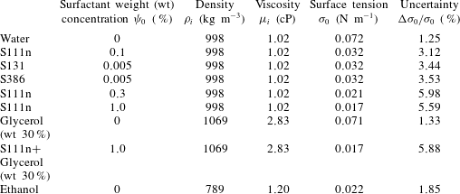
Three primary categories of surfactants have been tested in the experiments (Pan & Chen Reference Pan and Chen2012), i.e. anionic (S111n), amphoteric (S131) and non-ionic (S386), which are all soluble in water. The density and viscosity of the aqueous solutions are essentially identical, but the surface tension (
 ${\it\sigma}_{0}$
) changes significantly, as shown in figure 4, with the variation of initial surfactant concentration,
 ${\it\psi}_{0}$
. It is seen that
 ${\it\sigma}_{0}$
attains a minimum at the critical micelle concentration (CMC) limit, which designates the saturation level of surfactant on the liquid interface. These surfactants belong to a series of Surflon surfactants, produced by AGC Seimi Chemical Co., LTD. The surfactant, with a purity of
 $30\,\%$
, is a fluorochemical surface acting agent composed of perfluoroalkyl betaine. This product possesses excellent attributes that are not possible for hydrocarbon-based surfactants, such as a significant reduction in the surface tension with a small quantity added. While its viscosity is
 $8.8$
cP (
 $10^{-3}~\text{Pa}~\text{s}$
), the addition of a small amount does not substantially change the viscosity of its water solution. The properties of fluids tested in the study are listed in table 1. It is seen that, while surface tension is reduced ostensibly, viscosity is almost invariant after the surfactant is added to water. In contrast, when glycerol is added, the viscosity increases prominently while the surface tension stays essentially the same and density increases slightly.
In passing we note that, due to more data available for S111n in the broader range of transition before reaching the CMC limit, and hence more precise control of surface tension with addition of surfactant, as seen in the measurement in figure 4, most of the results presented are based on the surfactant S111n. While the ions on the droplet interfaces might induce certain effects, such a factor is shown to be insignificant for the key phenomena to be discussed in the following.
Variation of measured surface tension with surfactant concentration. The CMC limit of S111n is defined as
 ${\it\psi}_{0}\sim 0.35\,\%$
.

Properties of the tested fluids.

3 Mathematical model and numerical method
Numerical simulations are performed for multiphase fluid dynamics based on the immersed-boundary (IB) method (Peskin Reference Peskin1977). With conservation of specific mathematical and physical quantities, the surface forces are smeared to surrounding fluid grid points, so the computation can be carried out in a unified domain. This is generally known as an Eulerian–Lagrangian approach (Kuan, Pan & Shyy Reference Kuan, Pan and Shyy2014) for moving-boundary problems. In addition, the dynamics of soluble surfactant is calculated along with the conservation equations of fluid momentum and mass.
3.1 Governing equations
In this subsection, the mathematical model for head-on collision of two equal sized droplets with soluble surfactant in a three-dimensional (3-D) axisymmetric immersed-boundary formulation is described. We assume that, in the computational domain
 ${\it\Omega}=\{(r,z)|r\in (0,L_{r}),z\in (0,L_{z})\}$
, the two droplets are placed symmetrically with respect to
 $z=0$
(
 $r$
axis) so that the collision direction is along the
 $z$
axis. The fluid domain
 ${\it\Omega}$
consists of the droplet phase
 ${\it\Omega}_{i}$
and the surrounding fluid
 ${\it\Omega}_{o}$
(gas, throughout the report), and so in between there is an interface
 ${\it\Sigma}$
separating them. Mathematically, this interface is the boundary of
 ${\it\Omega}_{i}$
, i.e.
 ${\it\Sigma}=\partial {\it\Omega}_{i}$
. In this work, for insoluble surfactant, we mean that the surfactant exists only on the interface
 ${\it\Sigma}$
. For the present soluble case, however, the surfactant exists in the droplet domain
 ${\it\Omega}_{i}$
as well as the interface
 ${\it\Sigma}$
; thus we need to define two different concentrations (bulk concentration denoted by
 $C(\boldsymbol{x},t)$
and interfacial concentration denoted by
 ${\it\phi}(\boldsymbol{x},t)$
) as described later. The fluid interface
 ${\it\Sigma}$
separating the droplet and gas can be tracked in a Lagrangian manner
 $\boldsymbol{X}({\it\alpha},t)=(R({\it\alpha},t),Z({\it\alpha},t))$
with the parameter
 ${\it\alpha}$
ranging in
 $[0,1]$
. The unit tangent vector along the droplet interface is defined as
 ${\bf\tau}=({\it\tau}_{1},{\it\tau}_{2})=\boldsymbol{X}_{{\it\alpha}}/|\boldsymbol{X}_{{\it\alpha}}|$
with
 $|\boldsymbol{X}_{{\it\alpha}}|=\sqrt{R_{{\it\alpha}}^{2}+Z_{{\it\alpha}}^{2}}$
, where the subscript
 ${\it\alpha}$
indicates the partial derivative with respect to
 ${\it\alpha}$
. Therefore, the unit outward normal vector directing from the droplet
 ${\it\Omega}_{i}$
into the gas
 ${\it\Omega}_{o}$
can also be defined as
 $\boldsymbol{n}=({\it\tau}_{2},-{\it\tau}_{1})$
.
The immersed-boundary method (Peskin Reference Peskin2002) is a smoothing interface method that formulates the two-fluid problem into a unified one-fluid system by exploiting the indicator function Unverdi & Tryggvason (Reference Unverdi and Tryggvason1992) (or Heaviside function):
 $$\begin{eqnarray}\displaystyle H(\boldsymbol{x},t)=\int _{{\it\Omega}_{i}}{\it\delta}(\boldsymbol{x}-\boldsymbol{x}^{\prime })\,\text{d}\boldsymbol{x}^{\prime }. & & \displaystyle\end{eqnarray}$$
Here,
 $H=1$
represents the droplet phase (with the viscosity
 ${\it\mu}_{i}$
and density
 ${\it\rho}_{i}$
), while
 $H=0$
represents the gas phase (with
 ${\it\mu}_{o}$
and
 ${\it\rho}_{o}$
). Thus, this one-fluid system has viscosity and density defined by
 ${\it\mu}={\it\mu}_{i}H+{\it\mu}_{o}(1-H)$
and
 ${\it\rho}={\it\rho}_{i}H+{\it\rho}_{o}(1-H)$
, respectively. Another advantage of using the indicator function is to simplify the numerical procedure for solving the bulk surfactant concentration. In the present flow with soluble surfactant, the bulk concentration
 $C$
is defined only in the droplet phase
 ${\it\Omega}_{i}$
but not in
 ${\it\Omega}_{o}$
. One can redefine the bulk concentration by
 $HC$
so that the convection–diffusion equation for the bulk concentration is solved in the regular computational domain
 ${\it\Omega}$
rather than in the irregular non-stationary droplet domain
 ${\it\Omega}_{i}$
. Thus, we can regard
 $HC$
as the effective bulk surfactant concentration. The surfactant absorption and desorption between the bulk and interface can be termed as a singular delta source along the interface in our immersed-boundary framework. The above formulation for two-phase flow with soluble surfactant in two dimensions (2-D) can be found in detail in the recent work of Chen & Lai (Reference Chen and Lai2014). In the next section, we describe the governing equations for interfacial flow with soluble surfactant in a 3-D axisymmetric formulation.
Before we proceed, we introduce the mathematical definitions for the gradient, divergence and Laplace operators in axisymmetric cylindrical coordinates:
 $$\begin{eqnarray}\displaystyle \boldsymbol{{\rm\nabla}}=\left(\frac{\partial }{\partial r},\frac{\partial }{\partial z}\right),\quad \boldsymbol{{\rm\nabla}}\boldsymbol{\cdot }=\left(\frac{1}{r}\frac{\partial }{\partial r}r,\frac{\partial }{\partial z}\right),\quad {\it\Delta}=\boldsymbol{{\rm\nabla}}\boldsymbol{\cdot }\boldsymbol{{\rm\nabla}}=\frac{1}{r}\frac{\partial }{\partial r}\left(r\frac{\partial }{\partial r}\right)+\frac{\partial ^{2}}{\partial z^{2}}.\quad \qquad & & \displaystyle\end{eqnarray}$$
To compute the indicator function, one can first take the gradient operator for (3.1) and then apply the divergence operator to the resultant equation; so we obtain the following Poisson equation
 $$\begin{eqnarray}\displaystyle {\rm\Delta}H(\boldsymbol{x},t)=-\boldsymbol{{\rm\nabla}}\boldsymbol{\cdot }\int _{{\it\Sigma}}\boldsymbol{n}{\it\delta}(\boldsymbol{x}-\boldsymbol{X})\,\text{d}{\it\Sigma}. & & \displaystyle\end{eqnarray}$$
The non-dimensional Navier–Stokes flow with soluble surfactant in the usual immersed-boundary formulation can be written as
 $$\begin{eqnarray}\displaystyle & \displaystyle {\it\rho}\left(\frac{\partial \boldsymbol{u}}{\partial t}+(\boldsymbol{u}\boldsymbol{\cdot }\boldsymbol{{\rm\nabla}})\boldsymbol{u}\right)+\boldsymbol{{\rm\nabla}}p=\frac{1}{Re}\left(\boldsymbol{{\rm\nabla}}\boldsymbol{\cdot }{\it\mu}(\boldsymbol{{\rm\nabla}}\boldsymbol{u}+\boldsymbol{{\rm\nabla}}\boldsymbol{u}^{T})-\frac{{\it\mu}}{r^{2}}\boldsymbol{u}^{\ast }\right)+\frac{\boldsymbol{f}}{We}+\frac{{\it\rho}\boldsymbol{g}}{Fr^{2}}, & \displaystyle\end{eqnarray}$$
 $$\begin{eqnarray}\displaystyle & \displaystyle \boldsymbol{{\rm\nabla}}\boldsymbol{\cdot }\boldsymbol{u}=0, & \displaystyle\end{eqnarray}$$
 $$\begin{eqnarray}\displaystyle & \displaystyle \boldsymbol{f}=\int _{0}^{1}\boldsymbol{F}({\it\alpha},t){\it\delta}(\boldsymbol{x}-\boldsymbol{X}({\it\alpha},t))\,\text{d}{\it\alpha}, & \displaystyle\end{eqnarray}$$
 $$\begin{eqnarray}\displaystyle & \displaystyle \boldsymbol{F}({\it\alpha},t)=\frac{\partial }{\partial {\it\alpha}}({\it\sigma}({\it\phi}){\bf\tau}({\it\alpha},t))-{\it\sigma}({\it\phi})\frac{Z_{{\it\alpha}}}{R}\boldsymbol{n}({\it\alpha},t), & \displaystyle\end{eqnarray}$$
 $$\begin{eqnarray}\displaystyle & \displaystyle \frac{\partial \boldsymbol{X}({\it\alpha},t)}{\partial t}=\boldsymbol{U}({\it\alpha},t)=\int _{{\it\Omega}}\boldsymbol{u}(\boldsymbol{x},t){\it\delta}(\boldsymbol{x}-\boldsymbol{X}({\it\alpha},t))\,\text{d}\boldsymbol{x}, & \displaystyle\end{eqnarray}$$
 $$\begin{eqnarray}\displaystyle & \displaystyle \frac{\partial {\it\phi}}{\partial t}+(\boldsymbol{{\rm\nabla}}_{s}\boldsymbol{\cdot }\boldsymbol{u}){\it\phi}=\frac{1}{Pe_{s}}\frac{1}{R|\boldsymbol{X}_{{\it\alpha}}|}\frac{\partial }{\partial {\it\alpha}}\left(\frac{R}{|\boldsymbol{X}_{{\it\alpha}}|}\frac{\partial {\it\phi}}{\partial {\it\alpha}}\right)+{\it\Phi}({\it\alpha},t), & \displaystyle\end{eqnarray}$$
 $$\begin{eqnarray}\displaystyle & \displaystyle \frac{\partial (HC)}{\partial t}+\boldsymbol{{\rm\nabla}}\boldsymbol{\cdot }(\boldsymbol{u}HC)=\frac{1}{Pe}\boldsymbol{{\rm\nabla}}\boldsymbol{\cdot }(H\boldsymbol{{\rm\nabla}}C)-\int _{0}^{1}{\it\Phi}({\it\alpha},t){\it\delta}(\boldsymbol{x}-\boldsymbol{X}({\it\alpha},t))\,\text{d}{\it\alpha}. & \displaystyle\end{eqnarray}$$
 $\boldsymbol{u}=(u,w)$
defined on the domain
 ${\it\Omega}$
has the radial
 $u$
and axial component
 $w$
. In (3.4), an additional term in terms of
 $\boldsymbol{u}^{\ast }=(u,0)$
is introduced into the radial momentum equation, which arises from the cylindrical coordinate system. Equation (3.7) describes the immersed-boundary force arising from the surface tension
 ${\it\sigma}$
which depends on the interfacial surfactant concentration
 ${\it\phi}$
. A well-known model, the Langmuir equation of state (Eastoe & Dalton Reference Eastoe and Dalton2000; Ceniceros Reference Ceniceros2003; Lin et al.
Reference Lin, Lee, Yang and Liu2003), has been used extensively as the constitutive law to specify the relationship between surface tension
 ${\it\sigma}$
and surfactant concentration
 ${\it\phi}$
. However, the Langmuir model is not adequate for certain types of surfactant and can barely be used for low interfacial concentration. In this work, we shall use the data fitting to the experimental measurements for the particular surfactant S111n to obtain the constitutive function
 ${\it\sigma}({\it\phi})$
. The fluid interface,
 ${\it\Sigma}$
, simply moves with the local fluid velocity as shown in (3.8). The interaction between the Eulerian and Lagrangian variables is rendered by the Dirac delta function
 ${\it\delta}(\boldsymbol{x})={\it\delta}(r){\it\delta}(z)$
. The dimensionless numbers in the fluid equations are the Reynolds number (
 $Re={\it\rho}_{i}R_{0}U_{\infty }/{\it\mu}_{i}$
), the Weber number and the Froude number (
 $Fr=U_{\infty }/\sqrt{g_{\infty }R_{0}}$
). Here we define the characteristic scales by
 $R_{0}$
the radius of droplet at rest,
 $U_{\infty }$
the relative impact speed,
 ${\it\sigma}_{0}$
the clean surface tension and
 $g_{\infty }$
the gravitational constant.
Equations (3.9), (3.10) are the coupled convection–diffusion equations for the interfacial and bulk surfactant concentrations. In (3.9),
 $\partial /\partial t$
represents the material derivative since the interfacial surfactant
 ${\it\phi}({\it\alpha},t)$
is defined in the Lagrangian coordinate
 ${\it\alpha}$
. The surface gradient operator is defined as
 $\boldsymbol{{\rm\nabla}}_{s}=(\boldsymbol{I}-\boldsymbol{n}\boldsymbol{n})\boldsymbol{{\rm\nabla}}$
. Here, the coupled term
 ${\it\Phi}=S_{a}C_{{\it\Sigma}}(1-{\it\phi})-S_{d}{\it\phi}$
describes the absorption and desorption mechanisms between the interfacial and the bulk surfactant (Eggleton & Stebe Reference Eggleton and Stebe1998; Eastoe & Dalton Reference Eastoe and Dalton2000; Tabor, Eastoe & Dowding Reference Tabor, Eastoe and Dowding2009). This coupling ensures that the total surfactant mass is conserved mathematically. Here,
 $S_{a}$
and
 $S_{d}$
are the adsorption and desorption constants, respectively, and
 $C_{{\it\Sigma}}$
is the bulk surfactant concentration evaluated adjacent to the interface. To set the bulk surfactant concentration as zero in the gas, we take advantage of the indicator function so that
 $C_{{\it\Sigma}}$
can be simply evaluated by
 $$\begin{eqnarray}\displaystyle C_{{\it\Sigma}}({\it\alpha},t)=\int _{{\it\Omega}}HC{\it\delta}(\boldsymbol{x}-\boldsymbol{X}({\it\alpha},t))\,\text{d}\boldsymbol{x}. & & \displaystyle\end{eqnarray}$$
The dimensionless numbers for the surfactant equations are the bulk Peclet number
 $Pe=U_{\infty }R_{0}/D_{b}$
and surface Peclet number
 $Pe_{s}=U_{\infty }R_{0}/D_{s}$
, where
 $D_{b}$
and
 $D_{s}$
are the diffusivities of the bulk and interfacial surfactants, respectively. To make the present model well posed, we need proper boundary conditions for the velocity
 $\boldsymbol{u}$
and bulk concentration
 $C$
on
 $\partial {\it\Omega}$
, and initial conditions for
 $\boldsymbol{u}(\boldsymbol{x},0)$
,
 $C(\boldsymbol{x},0)$
,
 ${\it\phi}({\it\alpha},0)$
and the interface configuration
 $\boldsymbol{X}({\it\alpha},0)$
.
The short-range forces are formulated based on the well-known DLVO theory (Israelachvili Reference Israelachvili2011), named after Derjaguin, Landau, Verwey and Overbeek, which accounts for the combined effects of van der Waals (vdW) attractive force and EDL repulsive force. The classical description of such intermolecular forces (Zhang et al.
Reference Zhang, Xu, Jiang and Liu2010; Conlisk et al.
Reference Conlisk, Zambrano, Li, Kazoe and Yoda2012) arises from the Poisson–Boltzmann equation. By treating the thin film between the surfaces of two colliding droplets as a layer separating two identical charged, parallel planes, specifically around the annular rim where there is the smallest thickness of air gap and the curvature is relatively small (Pan et al.
Reference Pan, Law and Zhou2008), one can express the intermolecular forces per unit volume as the gradient of the corresponding disjoining pressure and insert it simply as a source term in the IB formulation, which is a function of the distance between the two planes. An approximation of the disjoining pressure,
 $p_{dj}=p_{vdw}+p_{edl}$
, is a combination of vdW effect,
 $p_{vdw}$
, and EDL effect,
 $p_{edl}$
, which are given in dimensional forms as
 $$\begin{eqnarray}\displaystyle p_{vdw}=-\frac{A_{0}}{6{\rm\pi}h_{g}^{3}},\quad p_{edl}=E_{0}\exp (-{\it\kappa}_{0}h_{g}),\quad E_{0}=64nkT\tanh ^{2}\left(\frac{z_{0}e{\it\varphi}}{4kT}\right),\quad & & \displaystyle\end{eqnarray}$$
where
 $h_{g}(r)$
is the width of the gap at
 $r$
,
 $A_{0}$
is the Hamaker constant (typically
 $10^{-21}$
to
 $10^{-19}$
J for water),
 $E_{0}$
is the Debye constant,
 ${\it\kappa}_{0}^{-1}$
is the Debye length (
 $960$
nm for water in liquid, which is approximately eight times smaller in air),
 $k$
is the Boltzmann constant,
 $T$
is the absolute temperature,
 $z_{0}$
is the charge number,
 $e$
is the elementary electron charge,
 $n$
is the ion concentration and
 ${\it\varphi}$
is the surface potential (Zhang et al.
Reference Zhang, Xu, Jiang and Liu2010). These two intermolecular factors affect the fluid-flow system through a volumetric force field in the dimensionless form as
 $$\begin{eqnarray}\displaystyle f_{molecule}=\frac{\partial p_{dj}}{\partial r}=\left(\frac{A}{{{\hat{h}}_{g}}^{4}}-E{\it\kappa}\exp (-{\it\kappa}{\hat{h}}_{g})\right)\frac{\partial {\hat{h}}_{g}}{\partial r}. & & \displaystyle\end{eqnarray}$$
Here the dimensionless Hamaker constant is
 $A=A_{0}/(2{\rm\pi}{\it\rho}_{i}R_{0}^{3}U_{\infty }^{2})$
and the Debye constant is
 $E=E_{0}/({\it\rho}_{i}U_{\infty }^{2})$
.
 ${\it\kappa}$
and
 ${\hat{h}}_{g}$
are normalized variables.
3.2 Numerical algorithm
In the numerical processes, all the fluid variables are defined at the cell centre labelled as
 $\boldsymbol{x}_{ij}=(r_{i-1/2},z_{j-1/2})=((i-1/2)h,c+(j-1/2)h)$
in
 ${\it\Omega}$
with the uniform mesh width
 $h$
in the
 $r$
and
 $z$
directions. It is noted that the uniform spatial grid used here is just for presentation purposes and it can be extended to a stretching grid without great difficulty in practice. For the immersed interface, we use a collection of discrete Lagrangian markers
 $\boldsymbol{X}_{k}=\boldsymbol{X}({\it\alpha}_{k})=(R_{k},Z_{k})$
to track the interface where
 ${\it\alpha}_{k}=k{\rm\Delta}{\it\alpha},k=0,1,\ldots ,M$
are the parametric points. Typically, the size of
 ${\rm\Delta}{\it\alpha}$
is chosen as
 ${\rm\Delta}{\it\alpha}\approx h/2$
. The discrete value
 $f_{k}$
denotes an approximation evaluated at
 ${\it\alpha}_{k}$
, while
 $f_{k+1/2}$
denotes the approximation evaluated at
 ${\it\alpha}_{k+1/2}=(k+1/2){\rm\Delta}{\it\alpha}$
. Using the standard centred-difference approximation, the unit tangent
 ${\bf\tau}_{k+1/2}$
, the unit normal
 $\boldsymbol{n}_{k+1/2}$
and the stretching factor
 $|\boldsymbol{X}_{{\it\alpha}}|_{k+1/2}$
are all evaluated at the half-integer index points. In addition, we also define the interfacial surfactant concentration
 ${\it\phi}_{k+1/2}$
and the surface tension
 ${\it\sigma}_{k+1/2}$
at those points with half-integer indices.
Let
 ${\rm\Delta}t$
be the size of the time step, and the superscript
 $n$
be the index. At the beginning of each time step, e.g. step
 $n$
, the interface configuration
 $\boldsymbol{X}_{k}^{n}$
, the fluid velocity
 $\boldsymbol{u}_{ij}^{n}$
, the interfacial surfactant concentration
 ${\it\phi}_{k+1/2}^{n}$
and the bulk concentration
 $C_{ij}^{n}$
must be given. Hence the complete numerical algorithm for solving (3.4)–(3.10) to advance one time step can be summarized as follows.
-
(1) Compute the surface tension
 ${\it\sigma}_{k+1/2}^{n}$
and unit tangent
${\bf\tau}_{k+1/2}^{n}$
, and then calculate the interface force
$\boldsymbol{F}_{k}^{n}$
as in (3.7).
-
(2) Distribute the interfacial force from the Lagrangian markers into the fluid as in (3.6) to obtain
$\boldsymbol{f}_{ij}^{n}$
. -
(3) Solve the Navier–Stokes equations (3.4), (3.5) by the projection method to update the new fluid velocity
$\boldsymbol{u}_{ij}^{n+1}$
. -
(4) Interpolate the new velocity on the fluid lattice points onto the marker point and move the marker point to update interface position
$\boldsymbol{X}_{k}^{n+1}$
as shown in (3.8). -
(5) Solve the equation (3.3) to obtain the new indicator function
$H_{ij}^{n+1}$
. -
(6) Solve the equation of interfacial surfactant concentration (3.9) to update
${\it\phi}_{k+1/2}^{n+1}$
. -
(7) Solve the bulk concentration equation (3.10) to update
$C_{ij}^{n+1}$
.


The above steps (1–4) are the conventional numerical procedures for the immersed-boundary method, for which the details are not reiterated. Readers who are interested in the numerical implementation in 2-D and 3-D axisymmetric Navier–Stokes flows with insoluble surfactant can find details in Lai et al. (Reference Lai, Tseng and Huang2008), Lai, Huang & Huang (Reference Lai, Huang and Huang2011). Here, we focus on the numerical steps (5–6) since the treatment of soluble surfactant is the main numerical topic of this paper.
In step (5), the indicator function can be discretized via the Poisson equation (3.3) directly using the centred-difference scheme by
 $$\begin{eqnarray}\displaystyle {\it\Delta}_{h}H_{ij}^{n+1}=-\boldsymbol{{\rm\nabla}}_{h}\boldsymbol{\cdot }\left(\mathop{\sum }_{k}\boldsymbol{n}_{k}^{n+1}{\it\delta}_{h}(\boldsymbol{x}_{ij}-\boldsymbol{X}_{k}^{n+1})|\boldsymbol{X}_{{\it\alpha}}|_{k}^{n+1}{\rm\Delta}{\it\alpha}\right), & & \displaystyle\end{eqnarray}$$
where
 ${\it\Delta}_{h}$
and
 $\boldsymbol{{\rm\nabla}}_{h}\boldsymbol{\cdot }$
are the standard centred-difference approximations for the Laplace and the divergence operators in axisymmetric cylindrical coordinates, respectively. The discrete delta function
 ${\it\delta}_{h}$
is adopted as the smoother one to avoid the oscillation of immersed force calculations, as introduced in Yang et al. (Reference Yang, Zhang, Li and He2009). The normal vector and the stretching factor evaluated at the marker
 $\boldsymbol{X}_{k}$
can be simply averaged by
 $\boldsymbol{n}_{k}=(\boldsymbol{n}_{k+1/2}+\boldsymbol{n}_{k-1/2})/2$
and
 $|\boldsymbol{X}_{{\it\alpha}}|_{k}=(|\boldsymbol{X}_{{\it\alpha}}|_{k+1/2}+|\boldsymbol{X}_{{\it\alpha}}|_{k-1/2})/2$
, respectively. The accuracy of the above numerical computation for the indicator function is well investigated in Chen et al. (Reference Chen, Feng, Kim and Lai2011).
To update the interfacial surfactant in step (6), we first rewrite the interfacial surfactant equation by multiplying the surface stretching factor
 $R|\boldsymbol{X}_{{\it\alpha}}|$
on both sides of (3.9). We then substitute the surface differential relation
 $\partial /\partial t(R|\boldsymbol{X}_{{\it\alpha}}|)=(\boldsymbol{{\rm\nabla}}_{s}\boldsymbol{\cdot }\boldsymbol{u})R|\boldsymbol{X}_{{\it\alpha}}|$
Lai et al. (Reference Lai, Huang and Huang2011) into the resultant equation to obtain
 $$\begin{eqnarray}\displaystyle \frac{\partial {\it\phi}}{\partial t}R|\boldsymbol{X}_{{\it\alpha}}|+\frac{\partial (R|\boldsymbol{X}_{{\it\alpha}}|)}{\partial t}{\it\phi}=\frac{1}{Pe_{s}}\frac{\partial }{\partial {\it\alpha}}\left(\frac{R}{|\boldsymbol{X}_{{\it\alpha}}|}\frac{\partial {\it\phi}}{\partial {\it\alpha}}\right)+{\it\Phi}({\it\alpha},t)R|\boldsymbol{X}_{{\it\alpha}}|. & & \displaystyle\end{eqnarray}$$
By applying the implicit Euler method for the time integration and using the centred-difference scheme for the spatial discretization, we have
 $$\begin{eqnarray}\displaystyle & & \displaystyle \frac{({\it\phi}R|\boldsymbol{X}_{{\it\alpha}}|)_{k+1/2}^{n+1}-({\it\phi}R|\boldsymbol{X}_{{\it\alpha}}|)_{k+1/2}^{n}}{{\rm\Delta}t}-{\it\Phi}_{k+1/2}^{n+1}(R|\boldsymbol{X}_{{\it\alpha}}|)_{k+1/2}^{n+1}\nonumber\\ \displaystyle & & \displaystyle \quad =\frac{1}{Pe_{s}{\rm\Delta}{\it\alpha}}\left(\frac{R_{k+1}^{n+1}}{|\boldsymbol{X}_{{\it\alpha}}|_{k+1}^{n+1}}\frac{{\it\phi}_{k+3/2}^{n+1}-{\it\phi}_{k+1/2}^{n+1}}{{\rm\Delta}{\it\alpha}}-\frac{R_{k}^{n+1}}{|\boldsymbol{X}_{{\it\alpha}}|_{k}^{n+1}}\frac{{\it\phi}_{k+1/2}^{n+1}-{\it\phi}_{k-1/2}^{n+1}}{{\rm\Delta}{\it\alpha}}\right),\end{eqnarray}$$
 $$\begin{eqnarray}\displaystyle & \displaystyle {\it\Phi}_{k+1/2}^{n+1}=S_{a}C_{k+1/2}^{\ast }(1-{\it\phi}_{k+1/2}^{n+1})-S_{d}{\it\phi}_{k+1/2}^{n+1}, & \displaystyle\end{eqnarray}$$
 $$\begin{eqnarray}\displaystyle & \displaystyle C_{k+1/2}^{\ast }=\mathop{\sum }_{ij}H_{ij}^{n+1}C_{ij}^{n}{\it\delta}_{h}(\boldsymbol{x}_{ij}-\boldsymbol{X}_{k+1/2}^{n+1})h^{2}. & \displaystyle\end{eqnarray}$$
 ${\it\phi}_{k+1/2}^{n+1}$
which can be solved very easily.
As for solving the bulk surfactant in step (7), we discretize (3.10) in a similar manner (implicit Euler method in time and centred-difference method in space) as in step (6) to obtain
 $$\begin{eqnarray}\displaystyle & \displaystyle \frac{(HC)_{ij}^{n+1}-(HC)_{ij}^{n}}{{\rm\Delta}t}+\boldsymbol{{\rm\nabla}}_{h}\boldsymbol{\cdot }(\boldsymbol{u}HC)_{ij}^{n}=\frac{1}{Pe}\boldsymbol{{\rm\nabla}}_{h}\boldsymbol{\cdot }(H\boldsymbol{{\rm\nabla}}_{h}C)_{ij}^{n+1}-\tilde{C}_{ij}^{n+1}, & \displaystyle\end{eqnarray}$$
 $$\begin{eqnarray}\displaystyle & \displaystyle \tilde{C}_{ij}^{n+1}=\mathop{\sum }_{k}{\it\Phi}_{k+1/2}^{n+1}{\it\delta}_{h}(\boldsymbol{x}_{ij}-\boldsymbol{X}_{k+1/2}^{n+1}){\rm\Delta}{\it\alpha}. & \displaystyle\end{eqnarray}$$
 ${\it\Phi}_{k+1/2}^{n+1}$
for all
 $k$
are already known from step (6), the above discretization involves solving a variable diffusion equation for the bulk concentration
 $C_{ij}^{n+1}$
. It is noted that, in practical numerical implementation, we need to regularize the diffusion coefficient (indicator function
 $H$
) by using
 $\sqrt{H^{2}+{\it\epsilon}^{2}}$
instead of
 $H$
simply because
 $H$
equals to zero in the gas phase
 ${\it\Omega}_{o}$
. Here,
 ${\it\epsilon}$
is chosen to be approximately
 $10^{-6}$
as suggested in Chen & Lai (Reference Chen and Lai2014).
3.3 Validation
The simulation is based on the similar methodology, i.e. the immersed-boundary method and front tracking, which has been applied in our previous studies for droplet related problems (Pan & Law Reference Pan and Law2007; Pan et al. Reference Pan, Law and Zhou2008). Substantial agreement regarding the evolution of deformed surfaces between the experiment and numerical simulation has been demonstrated, as also shown in the appendix A. Moreover, the advanced algorithm including surfactant dynamics is included in Chen & Lai (Reference Chen and Lai2014), in which a reasonable procedure of validation is performed. In addition, a convergence test along with the conservation of soluble surfactant is to be provided in § 5.2 with more discussion.
4 Experimental observation on impact outcome with addition of surfactant
The typical scenarios of droplet collision are shown in figure 2. Here the droplets of water generally merge at low/moderate Weber numbers and impact parameters (figure 2
a,b). Bouncing can only occur when the colliding path is significantly off centred, as shown in figure 2(c). At higher
 $We$
, after merging, separation of the coalesced droplets is created in order to balance the excess energy that cannot be contained in a single droplet. Stretching and reflexive (near head-on) forms of separation are observed in large (figure 2
d) and small
 $B$
(figure 2
e), respectively. With addition of surfactant, however, bouncing is generated even in head-on collision.
Figure 5 shows the regime diagram of droplet impacts. It is noted that, in the experiments, dimensional values such as surface tension are recorded. They will however be transformed to dimensionless quantities in order to be compared with computational results as discussed later. For pure water (figure 5
a), merging is the typical outcome right after collision, whether it is permanent at low
 $We$
or temporary coalescence at high
 $We$
, followed by separation of the merged droplet and further generation of satellite droplets. Bouncing of the impinging drops occurs only when
 $B$
is so large that the gas film remains in between and may act as a buffer to rebound the droplets. This regime was generally overlooked in early studies (Brazier-Smith et al.
Reference Brazier-Smith, Jennings and Latham1972; Ashgriz & Poo Reference Ashgriz and Poo1990; Jiang et al.
Reference Jiang, Umemura and Law1992), but was delineated in the study of Qian & Law (Reference Qian and Law1997). While nitrogen was used as the environmental gas, the regime reported therein was similar to the present one for which air was adopted, whose properties deviates little from that of nitrogen.
The regime diagram of impact on
 $(We,B)$
for (a) pure water with
 ${\it\sigma}_{0}=0.072$
 $\text{N}~\text{m}^{-1}$
; (b)
 ${\it\psi}_{0}=0.1\,\%$
surfactant S111n with
 ${\it\sigma}_{0}=0.032$
 $\text{N}~\text{m}^{-1}$
; (c)
 ${\it\psi}_{0}=0.3\,\%$
with
 ${\it\sigma}_{0}=0.021$
 $\text{N}~\text{m}^{-1}$
; (d)
 ${\it\psi}_{0}=1.0\,\%$
with
 ${\it\sigma}_{0}=0.017$
 $\text{N}~\text{m}^{-1}$
. The diameter of droplets was fixed at
 ${\sim}300~{\rm\mu}\text{m}$
except for pure water, which ranged from
 $280$
to
 $440~{\rm\mu}\text{m}$
. The impact velocity varied from
 $0.2$
to
 $2.6~\text{m}~\text{s}^{-1}$
. The symbols in the diagrams refer to the regimes as indicated in figure 1; here open circles indicate coalescence, stars bouncing and crosses separation. In (a), since the coalescence regimes at low
 $B$
are not intervened by the bouncing regime (II) created only at high
 $B$
, they are designated together by I/III.

By adding a small amount of surfactant, approximately
 $0.1\,\%$
(the initial mass fraction in a droplet, designated by
 ${\it\psi}_{0}$
), however, the bouncing regime (II) is substantially enlarged, as shown in figure 5(b). In particular, even in head-on collisions with
 $B=0$
, the droplets rebound after impact, which has never been observed for water. When more surfactant is added, as shown in figure 5(c) for a
 $0.3\,\%$
concentration of S111n, which is slightly below the CMC limit (see figure 4
a), the bouncing regime shows significant expansion. For a concentration far beyond the CMC limit, nevertheless, this regime is ostensibly shrunk, as shown in figure 5(d) for
 $1\,\%$
S111n.
Although the reduction in surface tension may play a role in such variations, as observed for other natural liquids such as hydrocarbons (Jiang et al.
Reference Jiang, Umemura and Law1992), it is not the major cause for the present cases with a surfactant. For demonstration, we have also adopted different surfactants (S131 and S386) while keeping surface tension fixed, so the mixture of water includes much less surfactant, i.e.
 $0.005\,\%$
, as shown in figure 6(a) for S386 that is non-ionic. In contrast to figure 5(b) for S111n, the bouncing regime is not enlarged much with the addition of these surfactants. However, when more surfactant is added (figure 6
b), specifically when approaching the CMC limit, remarkable expansion of the bouncing regime is again observed.
The experimental results reveal a predominant influence of the surfactant concentration, in addition to surface tension and the type of surfactant, which is related to the molecular structure of the chemical formulation and the effectiveness in reduction of surface energy. Such enhancement of rebounding between two aqueous droplets with surfactant can be understood by using numerical simulation for the correlations between the dynamics of the gas gap and the motions of fluids and surfactant.
The regime diagram of impact on
 $(We,B)$
for (a)
 ${\it\psi}_{0}=0.005\,\%$
surfactant S386 with
 ${\it\sigma}_{0}=0.032~\text{N}~\text{m}^{-1}$
; and (b)
 ${\it\psi}_{0}=1.0\,\%$
with
 ${\it\sigma}_{0}=0.021~\text{N}~\text{m}^{-1}$
. The diameter of droplets was fixed at
 ${\sim}300~{\rm\mu}\text{m}$
. The impact velocity varied from
 $0.2$
to
 $2.6~\text{m}~\text{s}^{-1}$
. The symbols in the diagrams refer to the regimes as indicated in figure 1.

Convergence test and the effect of surfactant solubility:
 $Re=213.6$
,
 $A=1.4255\times 10^{-11}$
,
 $We=8.9566$
and
 $Pe_{s}=100$
. The simulations with soluble surfactant consider additional parameters,
 $Pe=100$
 $S_{a}=2.32$
and
 $S_{d}=20$
. (a) Illustration of the deformed surfaces during impact, showing an exaggerated view of the gap between the droplets. (b) Grid refinement test based on the geometry and width of the gap at
 $t=1.0$
. (c) Evolution of
 $d_{r}$
for insoluble surfactant and soluble surfactant. (d) Evolution of surfactant mass. Here
 $M_{b}$
indicates the mass in the bulk fluid,
 $M_{s}$
is that on the surface and
 $M_{t}=M_{b}+M_{s}$
is the total mass in the system. (e) Distribution of interfacial surfactant concentration,
 ${\it\phi}$
, for insoluble (dash line) and soluble (solid line) cases at
 $t=0.5$
. (f) Distribution of Marangoni stress for insoluble (dash line) and soluble (solid line) cases at
 $t=0.5$
.

5 Computational analyses and discussion of observed results
Figure 7(a) illustrates the geometry of the collision between two droplets (one from the top and the other from the bottom), where
 $d_{c}$
and
 $d_{r}$
are indicated in a blow-up of the impact region. They are used to show the geometrical evolution of the gap expressed by the separation distance between the impinging surfaces (near the central plane which has a symmetric condition in the computation domain) of the two droplets at the centre and at the rim. It is noted that
 $d_{r}$
is measured at the radius where the minimum gap occurs, which is time dependent and is not measured at a fixed radius. As interpreted in Pan et al. (Reference Pan, Law and Zhou2008), the surfaces become indented when the droplets approach each other and pressure increases in the gap. The impedance due to the gap pressure is critical for the occurrence of bouncing, which is strongly related to the drainage of the trapped gas, and merging can happen only if the distance between the interfaces is reduced to such an extent that short-range factors are effective. Therefore, the smallest width of the gap computed based on the Navier–Stokes continuum mechanics could be identified as an index of tendency toward bouncing. In particular, if the minimum gap width that can be attained during the collision period, typically at the rim (and hence the smallest
 $d_{r}$
, as designated by
 $d_{r,min}$
), is much larger than the scale below which intermolecular attractive forces or other short-range mechanisms become dominant, the repulsive pressure yields rebounding of the droplets. The minimum gap width is changed by the addition of surfactant, which may induce the effects of reduced surface tension, non-uniform distributions of surfactant and repulsive EDL forces. They are investigated herein computationally based on the numerical simulation.
In this section, numerical parameters are selected from the experimental conditions. Instead of using dimensional quantities recorded for fluid properties in the experiments, the variables are non-dimensionalized in the presentation of computational results. First of all, a convergence test and a study of the capability of the numerical method in capturing the essential dynamics of surfactant-laden fluids are performed. Secondly, the concentration of surfactant is varied to identify the trend and the cause that prevents droplets from merging in collisions as observed in the experiments. A series of numerical tests related to the experimental situations of head-on collisions between droplets are conducted, including an investigation of the difference in using insoluble and soluble surfactants, which has been rare in the literature, and clarification of the surface tension effect. By means of such an a posteriori discussion, it is shown clearly that the key mechanism can be related to the Marangoni stress. Furthermore, consideration of a wide range in surfactant amount shows that the enhancement of the bouncing tendency has a limitation owing to the CMC limit of surfactant concentration. In addition, to understand the role of the other properties of the liquid played in such variations, specifically of viscosity, water droplets are mixed with glycerol to contrast the factor and show whether the observed bouncing regime due to the presence of surfactant is affected by viscosity.
5.1 Numerical set-up
The conditions of numerical tests are based on those of the experiments, where the radius of a spherical water droplet is
 $R_{0}=147.5~{\rm\mu}\text{m}$
and the impact speed is accelerated from zero by the gravitational field up to
 $U_{\infty }=1.48~\text{m}~\text{s}^{-1}$
. The density and viscosity of the droplets, respectively, are
 ${\it\rho}_{i}=998~\text{kg}~\text{m}^{-3}$
and
 ${\it\mu}_{i}=1020~{\rm\mu}\text{Pa}~\text{s}$
. The surface tension
 ${\it\sigma}_{0}$
of pure water in
 $1$
-atm regular air is approximately
 $0.072~\text{N}~\text{m}^{-1}$
, and the density and viscosity of air are respectively,
 ${\it\rho}_{o}=1.2~\text{kg}~\text{m}^{-3}$
and
 ${\it\mu}_{o}=18.6~{\rm\mu}\text{Pa}~\text{s}$
. Accordingly, the surface area, volume and mass of a droplet are
 $A_{d}=2.7340\times 10^{-7}~\text{m}^{2}$
,
 $V_{d}=1.3442\times 10^{-11}~\text{m}^{3}$
and
 $M_{d}=1.3415\times 10^{-8}$
kg, respectively.
These physical quantities are selected as the characteristic scales for normalization of the governing equations, and the relevant dimensionless numbers are
 $Re=213.6$
,
 $We=8.9566$
and
 $A=1.4255\times 10^{-11}$
. As discussed in Stebe, Lin & Maldarelli (Reference Stebe, Lin and Maldarelli1991), since the usual circumstance of mass transfer in liquids is characterized by high Peclet numbers, here we choose
 $Pe=Pe_{s}=100$
just for simplicity, as in Eggleton & Stebe (Reference Eggleton and Stebe1998) and Valkovska & Danov (Reference Valkovska and Danov2000). In addition, the selection of
 $S_{a}=2.32$
and
 $S_{d}=20$
are within the range of consideration in Zhang, Eckmann & Ayyaswamy (Reference Zhang, Eckmann and Ayyaswamy2006). Throughout this section, a computational domain
 ${\it\Omega}=[0,3]\times [0,3]$
is used in all numerical tests.
The experimental data of surface tension versus surfactant concentration were illustrated earlier in figure 4. Table 2 lists the variation of surface tension with surfactant (S111n) concentration in a static droplet. The amount of surfactant
 ${\it\psi}_{0}$
is measured as the percentage of its mass,
 $M_{d}$
, initially contained in a droplet. Figure 8 depicts the relation of the dimensionless surface tension
 ${\it\sigma}$
and interfacial concentration
 ${\it\phi}$
(for S111n) in terms of a polynomial fitting curve. It is seen that surface tension decreases dramatically in the beginning and then tends to level off after
 ${\it\psi}_{\infty }=0.35\,\%$
(see figure 4) which we name it as the maximum surfactant package. In this way, the dimensionless interfacial concentration of surfactant
 ${\it\phi}={\it\psi}_{0}/{\it\psi}_{\infty }$
is used for a given
 ${\it\psi}_{0}$
in the numerical processes and it is normalized to unity when CMC is attained. For instance, the mass concentration
 ${\it\psi}_{0}=0.1\,\%$
gives the value of
 ${\it\phi}=0.286$
.
According to table 2, the constitutive equation of
 ${\it\sigma}$
-
 ${\it\phi}$
can be approximated by a monotonic exponential model (dimensionless formulation):
 $$\begin{eqnarray}\displaystyle {\it\sigma}({\it\phi})=\left\{\begin{array}{@{}ll@{}}0.754e^{-3.45{\it\phi}}+0.246, & {\it\phi}<1\\ 0.270, & {\it\phi}\geqslant 1.\end{array}\right. & & \displaystyle\end{eqnarray}$$
Curve fitting for the experimental data of S111n in figure 4. The solid line is formulated by a monotonic exponential model and the diamond markers indicate the non-dimensionalized data of S111n.

Since the data in table 2 were measured at steady state, we simply assume that all the surfactant already attached to the interface when
 ${\it\psi}_{0}<{\it\psi}_{\infty }$
, and the corresponding
 ${\it\phi}$
is simply
 ${\it\psi}_{0}/{\it\psi}_{\infty }$
. If
 ${\it\psi}_{0}>{\it\psi}_{\infty }$
, the surface has reached the maximum package filled with surfactant and the remainder are dissolved into the droplet. For instance, if we add
 $0.5\,\%$
surfactant into the droplet, then
 ${\it\phi}_{0.5\,\%}=1$
and
 $C_{0.5\,\%}=3/7$
.
Experimental measurement of surface tension
 ${\it\sigma}_{0}$
(
 $\text{mN}~\text{m}^{-1}$
) versus S111n surfactant fraction (
 ${\it\psi}_{0}$
, mass percentage of
 $M_{d}$
). The relative error of the monotonic exponential fitting according to (5.1),
 $|e_{{\it\sigma}}|$
, is also shown. Here
 $|e_{{\it\sigma}}|$
is defined as
 $({\it\sigma}_{exp}-{\it\sigma}_{fit})/{\it\sigma}_{exp}$
, where
 ${\it\sigma}_{exp}$
is the dimensionless surface tension obtained from the experiment while
 ${\it\sigma}_{fit}$
is that from the monotonic exponential model.
 ${\it\sigma}_{fit}$
is fixed at
 $0.754e^{-3.45}+0.246$
as
 ${\it\psi}_{0}>0.35\,\%$
.

5.2 Convergence test, solubility and mass conservation
To understand evolution of the intervening gap during droplet collision, we define two characteristic distances; namely,
 $d_{c}$
(gap at the centre) and
 $d_{r}$
(gap at the rim), which are used to present the gap dynamics. Figure 7(a) shows the impact diagram of two droplets. The code is validated through a mesh refinement process, and the convergence of the numerical method is explained by the profile of droplet surface at
 $t=1.0$
which is approximately the time when the minimum gap is attained. Figure 7(b) shows three profiles of the deforming gap with minimum mesh sizes
 $4h$
,
 $2h$
and
 $h$
, respectively, where a linear convergence is observed. It is noted that, with variation of the gap size,
 $d_{r}$
, at least two cells are always kept in between two interfaces, particularly at the rim, such that the IB calculation is valid.
To gain an insight into the effect of surfactant solubility on the dynamics of droplet collision we consider two cases, both having
 ${\it\psi}_{0}=0.1\,\%$
(so
 ${\it\phi}=0.286$
) surfactant inserted but one is soluble and the other is insoluble. Figure 7(c) shows the gap dynamics before
 $t=3.0$
. The dashed line represents the evolution of
 $d_{r}$
in the insoluble case and the solid line represents the result of the soluble case. Obviously, the insoluble case has a bigger gap size at the rim, as compared to that of the soluble case. A reasonable explanation is that the insoluble case keeps all surfactant on the interface such that a stronger Marangoni stress (compared to the soluble case) due to non-uniform distribution of surfactant concentration suppresses more the air drainage during the collision (to be interpreted further in the next section). The corresponding distributions of surfactant concentration and Marangoni stress at
 $t=0.5$
are shown in figure 7(e,f), respectively. It is seen that large amplitudes appear in both cases outside the rims of the deformed droplet surfaces, which are indicated by circular markers. Specifically, the negative stresses closer to the rims indicate the inward direction of surfactant induced forces that would prevent the air flow in the gap from draining out, as will be further demonstrated.
To further test the numerical accuracy and solubility of surfactant, we have examined the natural oscillation of a droplet for cases with insoluble and soluble surfactant. The oscillation period is predicted for a clean droplet as
 $T_{0}=2{\rm\pi}(\!{\it\rho}_{i}R_{0}^{3}/8{\it\sigma}_{0}\!)^{1/2}$
(Lamb Reference Lamb1932), based on an inviscid condition with small oscillation amplitude. With surface tension set identically to
 $0.032~\text{N}~\text{m}^{-1}$
at the beginning, when surfactant is uniformly distributed in the droplet for both cases, the oscillation periods are the same, i.e.
 $T_{0}\sim 7.0277\times 10^{-4}$
s. As time passes however, the soluble case exhibits a shorter duration,
 $T_{0}=5.9797\times 10^{-4}$
s. This can be reasonably explained by the reduction of interfacial concentration, hence increase of surface tension, due to the solubility of surfactant.
Figure 7(d) shows the evolutions of
 $M_{b}$
(the surfactant mass in the bulk fluid),
 $M_{s}$
(the surfactant mass on the interface) and the total mass
 $M_{t}$
of the system. Due to the solubility of surfactant, the mass on the interface
 $M_{s}$
(dashed line) decreases with time while the mass in the bulk fluid
 $M_{b}$
(dotted line) increases. Since the mass-preserving numerical scheme guarantees perfect conservation of surfactant mass with minimum roundoff error in a discrete sense through summation by parts, the total mass
 $M_{t}$
remains invariant for both soluble and insoluble cases, and the two curves of evolution overlap.
5.3 Marangoni effect due to surfactant
In order to clarify the key factors that cause the water droplets to bounce off instead of coalescence in the presence of surfactant, we first focus on the magnitude of dimensionless surface tension,
 ${\it\sigma}$
. Variation of surface tension along the droplet interfaces may induce effects of both capillary stress and Marangoni stress. To identify these using computational analysis, we test two cases for clean droplets (no surfactant), i.e. one with
 ${\it\sigma}=1$
and the other with
 ${\it\sigma}=0.41$
. The effects can be demonstrated via the variations in the neighbourhood of the thin air film between the deformed surfaces, which is closely related to the drainage of fluid in between. The measurements of the minimum distance at the rim
 $d_{r}$
and the distance at the centre
 $d_{c}$
can provide such crucial information as to reveal the possibility of the draining out of sufficient air in a timely manner and to encourage further approaching of the surfaces. In the present simulation for droplet collision, however, due to the domain boundary condition and finite grid resolution, coalescence of the interfaces will not happen spontaneously without inclusion of any short-range mechanisms such as the vdW attractive force. Therefore, an artificial vdW effect is considered in this section, which yields the possibility to evaluate droplet merging based on the separation distance.
Simulations of droplet impact dynamics with varied surface tension (
 ${\it\sigma}=1,0.41$
) in the absence of surfactant (
 ${\it\phi}=0$
), showing evolution of (a)
 $d_{c}$
and (b)
 $d_{r}$
. Simulations of droplet impact dynamics involving fixed surface tension (
 ${\it\sigma}=0.41$
) but with (
 ${\it\phi}=0.286$
) or without surfactant (
 ${\it\phi}=0$
), showing evolution of (c)
 $d_{c}$
and (d)
 $d_{r}$
.

Figure 9(a,b) shows the evolution of two separation distances between the droplets during the impact in terms of the dimensionless variables. The solid line is for the water droplet with
 ${\it\sigma}=1$
, and the dash line is for the droplet with
 ${\it\sigma}=0.41$
. The latter case has smaller surface tension, which means a smaller capillary force, so that the corresponding interface is softer and easier to deform. The maximum pressure occurs at the central position, and hence
 $d_{c}$
is always larger than
 $d_{r}$
, indicating that the impinging surface of the droplet is indented by the pressure built up in the gas gap. This indentation is manifested, as indicated by lower
 $d_{r}$
and higher
 $d_{c}$
(due to incompressibility of liquid), when the dimensionless surface tension is reduced to
 ${\it\sigma}=0.41$
, as compared to
 ${\it\sigma}=1$
for pure water. As a consequence, the separation distance between the rims of the impinging surfaces becomes smaller; therefore, the case is more subject to short-range attraction and merging. This demonstrates that the decrease in surface tension, though resulting in greater deformation of the droplet surface, should not be a key factor for the enhancement of bouncing when a surfactant is added. A similar effect is seen in Purvis & Smith (Reference Purvis and Smith2004) regarding a droplet impacting a surface, which reports that inclusion of surface tension can increase the gap separation and delay touchdown. While not being exactly identical to the present discussion considering the gap deformation, it indicates a consistent tendency of enhanced bouncing with increased surface tension as demonstrated herein.
Next, to examine the effect of adding surfactant, we rewrite (3.7) as
 $$\begin{eqnarray}\displaystyle \boldsymbol{F}({\it\alpha},t)=\frac{\partial {\it\sigma}({\it\phi}({\it\alpha},t))}{\partial {\it\alpha}}{\bf\tau}({\it\alpha},t)+{\it\sigma}\left(|\boldsymbol{X}_{{\it\alpha}}|{\it\kappa}-\frac{Z_{{\it\alpha}}}{R}\right)\boldsymbol{n}({\it\alpha},t), & & \displaystyle\end{eqnarray}$$
which is the combination of tangential stress and normal stress, as indicated by the first and second terms, respectively. Injecting surfactant into the droplets renders not only a reduction of surface tension (normal stress) but also a non-uniform distribution of surface tension (tangential stress). In this case, the water droplet contains
 ${\it\phi}=0.286$
surfactant, hence with a concentration lower than the maximum allowed on the surface. Since the surfactant attaches uniformly to the droplet surface in the beginning, the resulting surface tension is
 ${\it\sigma}=0.41$
. By keeping identical surface tension in a clean droplet without surfactant, we can isolate the influence of capillary stress and identify the variation due to non-uniform surfactant distribution. Consequently, as demonstrated in figure 9(c,d), substantial increases in both
 $d_{r}$
and
 $d_{c}$
are observed when soluble surfactant is included. Such an increase in the gap width leads to a higher tendency to rebound, as shown for the case of
 ${\it\phi}=0.286$
, which then completes the cycle after exhibiting a converging of
 $d_{r}$
and
 $d_{c}$
due to the ‘buckling’ of the indented surface at a later stage. As discussed in Pan et al. (Reference Pan, Law and Zhou2008), the indented surface recovers rapidly to a nearly prolate shape when the droplet bounces off and so the location with minimum separation distance switches back to the centre of the impinging surface, as observed at the beginning of the impact. The non-uniform distribution of surfactant concentration shows an aggregation of surfactant outside the rim, see figure 7(e). This causes smaller surface tension and consequently a sharp positive gradient of surfactant concentration accompanied by a sharp negative gradient of surface tension which yields a Marangoni stress acting in the tangential direction from outside of the rim into the gap. In contrast to the Marangoni flow frequently observed, such a mechanism leads to suppression of outward fluid motion in the draining process of droplet impact. Consequently, more air is trapped in the gap and the separation distance between the interfaces becomes larger; this discourages merging of the droplets and hence may result in bouncing, as observed in the experiments. To further understand and demonstrate the role of the Marangoni effect, various factors are investigated computationally.
In the following, the effects of intermolecular forces (Jiang & James Reference Jiang and James2007) on the film dynamics at small scale are considered, including the attractive vdW force and repulsive EDL force that could be incurred by the anionic surfactant S111n. Instead of measuring or calculating the value of
 $E$
directly, which is usually unattainable due to inherent complications, we assume that the EDL effect and vdW effect are comparable within a small range of separation distance,
 ${\hat{h}}_{g}$
, while the former is generically weaker than the latter unless
 $h_{g}$
is very small, usually less than O(
 $10$
nm). From (3.13), we rewrite
 $E$
as a function of
 ${\hat{h}}_{g}$
such that the dimensionless Debye constant is approximated by
 $E\sim A/({\it\kappa}{{\hat{h}}_{g}}^{4}\exp (-{\it\kappa}{\hat{h}}_{g}))<0.0295$
. Here
 ${\hat{h}}_{g}>2h_{min}$
and
 ${\it\kappa}=1.23\times 10^{3}$
. It is noted that the lower bound
 $h_{min}$
is the finest mesh size in the
 $z-$
direction in the numerical tests. Since the gap between two droplets never reaches
 $2h_{min}$
in the cases of bouncing and
 ${\it\kappa}^{-1}\approx 8\times 10^{-4}>2h_{min}$
, we can approximate
 $E$
by using figure 10(a).
Simulations of gap evolution with intermolecular effects. (a) Variation of dimensionless Debye constant
 $E$
versus gap size. Evolutions of
 $d_{r}$
showing (b) comparison of gap width with the Marangoni effect (solid line) and with an unrealistic repulsive EDL effect (dashed line); (c) variation of gap width at constant
 ${\it\phi}=0.286$
(
 ${\it\psi}_{0}=0.1\,\%$
) with varied Debye constant rendering attractive EDL effect; (d) variation of gap width at constant
 ${\it\phi}=0.286$
with varied Hamaker constant rendering attractive vdW effect.

Considering first the case including the attractive vdW effect only, it is confirmed in figure 10(d) that, unless the vdW force is unrealistically large, the repulsion due to the Marangoni effect can never be overcome and the droplets always rebound. It is observed that the results for
 $A=10^{-11}$
and
 $A=10^{-7}$
are basically the same as those with
 $A=0$
(hence not shown). Since the dimensionless Hamaker constant of water (
 $A$
) is up to
 $10^{-11}$
, the attractive force requires an augmentation of approximately five orders of magnitude (
 $10^{-6}$
) to yield a continual decrease in
 $d_{r}$
and, thus, high preference for coalescence. Therefore, with a gap width computed based on Navier–Stokes continuum flow dynamics, the pressure shall resist further approaching of the droplet surfaces before the short-range attraction becomes effective at a much smaller distance. This is caused solely by the dynamic distribution of surfactant around the surface, which yields non-uniform concentrations of surfactant and, hence, Marangoni stresses due to the gradients of surface tension. Upon impact, the convective flow created inside the droplet drives surfactant outward along the impinging surface, leading to decreasing concentration and increasing surface tension around the centre region of the film. As shown in figure 7(f) for
 ${\it\phi}=0.286$
, a negative Marangoni stress is then generated near the rim of the droplet surface, where a larger curvature is created and the liquid flow convected from the centre is about to turn upward; consequently, the inward force suppresses the drainage of gas out of the gap. This yields a wider gap between the colliding surfaces of droplets and discourages coalescence. The draining rate of the gas flux, which is similar to a plug flow, correlated with these factors is demonstrated later.
The effect and significance of EDL forces are demonstrated in figure 10(b,c). In figure 10(b), we compare the processes of interface separation, eventually leading to bouncing, due to the Marangoni effect and repulsive EDL effect. The solid line designates the case with surfactant concentration
 ${\it\phi}=0.286$
in the absence of the EDL effect (
 $E=0$
). Without surfactant, the other case indicated by the dashed line is concerned merely with the EDL effect on the tendency leading to bouncing of impact droplets. It shows that, without exhibition of any surfactant effect, even with an augmented Debye constant
 $E$
as large as
 $100$
, which is much larger than the typical value,
 $E\sim 0.0295$
, which has been somewhat overestimated, the minimum gap width yielded by the repulsive EDL force alone is still smaller than that caused by the Marangoni effect, as
 ${\it\phi}=0.286$
. No visible deviation is observed for cases with
 $E<10$
. It is observed that the repulsive EDL effect may enhance the bouncing tendency when
 $E$
is approximately
 $100$
, but is still weaker than the Marangoni effect and not strong enough to noticeably cause rebounding.
To further demonstrate the significance of the EDL effect as compared to the surfactant effect that encourages bouncing, the EDL force is inverted and so becomes ‘attractive’, and the droplet is subjected simultaneously to the Marangoni stress with
 ${\it\phi}=0.286$
. In the case with attractive EDL force, negative Debye constants are considered in droplet collision with surfactant, as shown in figure 10(c). It is seen that the minimum distances at the rim (
 $d_{r}$
) and at the centre (
 $d_{c}$
, not shown) are only slightly displaced even with
 $E$
as high as
 $100$
. The Debye constant must increase exaggeratedly to
 $1000$
so that the EDL force can dominate over the Marangoni effect, thereby the separation distance between the interfaces continues to decrease and coalescence may occur; this is unlikely to be created in reality since the magnitude is approximately five orders larger than the typical value.
These results indicate that only unrealistic Debye constants will render a pronounced effect on droplet rebounding in the present problem and, therefore, the EDL effect is not responsible for the enlargement of the bouncing regime as observed experimentally. At the length scale of the gas gap reached during the impinging and before the droplets can overcome the repulsion due to the Marangoni effect and the pressure built up in the gap such that the surfaces can approach each other further, therefore, the intermolecular forces are not effective enough to change the inclination to bouncing.
5.4 Influence of surfactant concentration
The effect of surfactant concentration is studied for different values of
 ${\it\psi}_{0}$
(and also
 ${\it\phi}$
, whereas it remains constant over CMC). We increase the amount of surfactant from less than the CMC limit to that over the CMC limit and examine the variation of gap dynamics accordingly with varied Marangoni stress as well as the distribution of interfacial concentration.
Variations of interfacial properties with increasing surfactant concentration from below to above the CMC limit (
 ${\it\psi}_{0}\sim 0.35\,\%$
). Evolution of
 $d_{r}$
with surfactant concentration (a) below the CMC limit:
 ${\it\phi}=0.286$
(
 ${\it\psi}_{0}=0.1\,\%$
, dashed line) and
 ${\it\phi}=1$
(
 ${\it\psi}_{0}=0.35\,\%$
, solid line); (b) above the CMC limit:
 ${\it\phi}=1$
(
 ${\it\psi}_{0}=0.35\,\%$
, solid line) and
 ${\it\phi}=1$
(
 ${\it\psi}_{0}=1\,\%$
, dash-dot line). The insets show the evolutions of
 $d_{c}$
. (c) Distribution of interfacial concentration,
 ${\it\phi}$
, versus arclength, at
 $t=0.5$
. (d) Distribution of tangential stress along the arclength at
 $t=0.5$
. The circular marker indicates the position of the rim in terms of arclength, where the separation distance is smallest.

As shown in figure 11(a), with surfactant concentration lower than the CMC limit (e.g. for
 ${\it\phi}=0.286$
and
 ${\it\phi}=1$
), the separation distance between the impinging surfaces of droplets is enlarged with increasing amount of surfactant, as indicated both by
 $d_{r}$
and
 $d_{c}$
. When surfactant concentration is higher than the CMC limit (here both
 ${\it\phi}=1$
but
 ${\it\psi}_{0}=0.35\,\%$
and
 $1.0\,\%$
), however, the separation distance is reduced with increasing amount of surfactant, as seen in figure 11(b). In these cases, surfactant is carried mainly by the convected flow within the droplet toward the area outside the rim of the thin film, as indicated by the peak of high concentration in figure 11(c). Such a mechanism subsequently yields large gradients of surfactant concentration along the droplet surface. In the meantime, part of the surfactant on the surface is dissolved in the bulk fluid of the droplet. As a consequence, surface tension is changed along the interface and tangential stress, specifically of negative sign which indicates a force toward the centre, is generated conspicuously on the impinging droplet surface due to the Marangoni effect, as shown in figure 11(d). We also note that, since addition of more surfactant leads to higher concentration and lower surface tension, the surface becomes softer and larger deformation results; consequently, the draining and rebounding processes last longer, as shown by the tails in figure 11(a,b).
The variation of Marangoni stress with increasing surfactant concentration is further demonstrated in figure 12, at an early instant when substantial deformation of the droplet surface is formed and a thin gas film is created. Here, the distribution of tangential stress is manifested as superimposed on the contour of the droplet surface in the three-dimensional plots. It is seen that with an increase of
 ${\it\phi}$
, when it is below the CMC limit, a larger Marangoni stress is formed due to the higher concentration of surfactant on the interface. When the interfacial concentration of surfactant is over the CMC limit (
 ${\it\phi}=1$
), the inward Marangoni stress decreases with increasing
 ${\it\psi}_{0}$
(while still
 ${\it\phi}=1$
). This is because the interface is already saturated with surfactant at the beginning when the droplet is spherical and even as
 ${\it\phi}$
becomes lower than one locally on the droplet surface when it is deformed later, particularly near the rim, more surfactant from the bulk fluid can refill the deficit and reduce the difference of surfactant concentration along the surface. In contrast, for the cases below the CMC limit with
 ${\it\phi}<1$
, since not much surfactant is dissolved in the bulk fluid, the concentration difference along the interface can be readily yielded by the non-uniform distribution due to the dynamics of convection and diffusion. In this case, the interfacial gradient of surface tension is not compromised much by the surfactant within the droplet.
Three-dimensional plots showing the distributions of Marangoni stresses (the gradient of surface tension) along the droplet surface at selected instants for surfactant concentrations below and around the CMC limit (
 ${\it\psi}_{0}\sim 0.35\,\%$
, solid line) at
 $t=0.4$
(b), and those near the CMC limit and above, at
 $t=0.375$
(c). Only the right half of the upper droplet is plotted (cf. the configuration shown in (a), as marked by the rectangles), as expressed by the half-ellipse (blue dotted line) on the
 $r$
–
 $z$
plane of the 3-D plot. It is seen that negative peaks are created on the impinging (lower) surface near the annular rim of the gas gap.

Formation of the Marangoni stress subsequently results in the variation of flow dynamics around the gas gap between the droplets and drainage of the interstitial gas which plays a key role in the propensity of droplet rebounding. To demonstrate the draining rate of flow in the gas gap, we calculate the evolution of outward volumetric flux by
 $$\begin{eqnarray}\displaystyle {\it\zeta}(t)=\int _{0}^{Z_{m}(t)}u(r_{m}(t),z)r_{m}(t)\,\text{d}z, & & \displaystyle\end{eqnarray}$$
where
 $r_{m}$
is the closest
 $r$
-coordinate at which the minimum gap is established, and
 $(R_{m}(t),Z_{m}(t))$
are the Lagrangian coordinates of the corresponding interfacial point. As seen in figure 13 for the evolution of
 ${\it\zeta}$
, at the early stage of droplet impact (before
 $t=0.4$
), since the minimum gap occurs at the centre of the impinging droplet surface (
 $r=0$
), there is not much difference for various surfactant concentrations,
 ${\it\psi}_{0}$
. While the flow convection in the droplet yields a slight difference in surfactant concentration near
 $r=0$
, such a small deviation does not yield a significant difference in the draining flow rate with variation of surfactant amount in the droplet.
Evolution of outward volumetric flux at the rim of the gas gap with various surfactant concentrations (
 ${\it\psi}_{0}$
). The corresponding evolutions of
 $d_{r}$
are also shown in the inset for comparison.

When the minimum gap switches from the centre to the rim (
 $t\sim 0.4$
) due to the growth of pressure and hence dimpling at the centre, the flow drainage is affected substantially by the non-uniform distribution of surfactant that is particularly manifest near the opening of the gap where the width is minimum. Within the small gap between the colliding interfaces, the flow is essentially a plug flow (Nobari, Jan & Tryggvason Reference Nobari, Jan and Tryggvason1996) and no complex flow structure, such as recirculated flow, is observed in the simulation. As demonstrated in figures 11 and 12, the change of surfactant concentration produces a local minimum of surface tension, rendering a Marangoni stress whose orientation is opposite to that of flow draining. Such a mechanism would not reverse the direction of fluid drainage but serve as a resistance for reducing the draining efficiency; this is demonstrated by a lower flux when the Marangoni stress becomes stronger with increasing
 ${\it\psi}_{0}$
, as shown in figure 13. The trend, however, is reversed as
 ${\it\psi}_{0}$
is over the CMC limit and further increased, for which the supply of surfactant from the bulk fluid mitigates the non-uniformity on the droplet surface and hence reduces the effect of Marangoni stress. These variations of flow draining rate after an annular rim is formed (
 $t>0.4$
, but before
 $t\sim 0.6$
when the droplets rebound) thus lead to the changes of minimum gap width with varied
 ${\it\psi}_{0}$
and justify the physical mechanisms of Marangoni effects on causing these trends as discussed.
These results can hence be used to interpret the phenomena observed in the experiments as illustrated in figure 5, showing broadening of the bouncing regime with increase of initial surfactant amount below the CMC limit and shrinking of this regime above the CMC limit. In addition, clearer elucidation is thus provided for the occurrence of larger gap size in the insoluble case compared to the result of soluble surfactant, as discussed for figure 7.
The impact regime diagram
 $(We,B)$
for water droplets mixed with (a)
 $30\,\%$
glycerol (
 ${\it\sigma}_{0}=0.072~\text{N}~\text{m}^{-1}$
), and (b)
 $30\,\%$
glycerol plus surfactant S111n with
 ${\it\psi}_{0}=1.0\,\%$
(
 ${\it\sigma}_{0}=0.017~\text{N}~\text{m}^{-1}$
). The diameter of droplets was
 ${\sim}440~{\rm\mu}\text{m}$
. The impact velocity varied from
 $0.2$
to
 $2.6~\text{m}~\text{s}^{-1}$
. The symbols in the diagrams refer to the regimes as indicated in figure 1.

The present illustration of the experimental and computational results on binary droplet collision showing variation of non-uniform distribution of surfactant and induced forces with embedded concentration is in accordance with the appearance of a remobilization regime discussed in Stebe et al. (Reference Stebe, Lin and Maldarelli1991). In the latter study, experimental evidence was presented in terms of a capillary train flow of alternating aqueous and gas slugs moving over a fluorocarbon wetting layer, which indicated that the interfaces of moving fluid particles can remain unhindered in the presence of a single adsorbed surfactant if it has fast desorption kinetics relative to surface convection and is present in sufficiently high bulk concentration. Under such circumstance, loss of mobility of the interface due to retarding forces caused by impurity of surfactant on the surface may degenerate and the local flow can regain mobility when the concentration gradients are reduced. With increase of surfactant concentration, specifically over the CMC, the droplet surface could be remobilized and behave like one without a Marangoni effect but only with reduced surface tension. We have experimentally increased surfactant concentration to even higher level, i.e. to
 $2\,\%$
and
 $5\,\%$
, and found that the bouncing regime indeed appeared to shrink as discussed. Nonetheless, when much more surfactant was added, e.g.
 $9.8\,\%$
, the system became unstable and difficult to analyse, possibly due to the sophisticated rheological effects of largely increased micelles and deterioration of the surfactant stored for a long duration. The issue may appear complicated and would be another topic of study for which we have been conducting related research regarding concentration and category.
5.5 Variation of droplet rebounding due to viscous effect
To further investigate the effects of other fluid properties on the transition boundaries, we have performed experiments with varied viscosity by adding glycerol. As indicated by the measured data in table 1, adding
 $30\,\%$
glycerol to the water droplets yields a pronounced increase of viscosity, which is almost tripled, while surface tension remains invariant. It is however shown in figure 14(a) that substantial increase of viscosity does not change much the bouncing regime, though its influence is reflected in the somewhat lowered impact parameter due to reduced mobility of the droplet surfaces and hence less effective draining of the intervening gas. If surfactant is added, as shown in figure 14(b), this regime is prominently expanded, as observed in the cases without glycerol. This again demonstrates the significant effect of surfactant on rebounding of droplets. Such an effect could not be simply characterized by the known dimensionless numbers such as the Ohnesorge number (
 ${\sim}{\it\mu}_{i}/\sqrt{{\it\rho}_{i}{\it\sigma}_{0}D_{0}}$
) or capillary number. The large increase of viscosity due to glycerol has changed substantially the Ohnesorge number whereas the regime boundary of bouncing is almost invariant, in contrast to the sensitive variation caused by addition of surfactant. While the latter lowers surface tension as well, the consequence is not the main cause for enhancement of the rebounding as demonstrated computationally in § 5.3. This is further justified by the experiment using ethanol droplets. It is shown in figure 15 that, even with surface tension as low as that given by the CMC limit, regime II of ethanol is not extended much so as to intersect the axis of
 $B=0$
and create bouncing in the head-on condition as observed when using surfactant solution. While the viscosity is somewhat higher than that of water and its mixture with surfactant, its influence should be relatively weak as discussed for glycerol. The effect of lower density of liquid is not fully understood at this moment and would be another topic of further study. Regarding the smaller extent of difference and resulting variation in bouncing tendency, however, its dominance should not outweigh the effects of non-uniform surfactant distribution and relatively larger reduction of surface tension.
The impact regime diagram
 $(We,B)$
for ethanol droplets (
 ${\it\sigma}_{0}=0.022~\text{N}~\text{m}^{-1}$
). The diameter of droplets was
 ${\sim}450~{\rm\mu}\text{m}$
.

These variations are investigated via computational analyses as well. Figure 16(c) shows evolutions of the air gap between impact droplets made of pure water and water solution with
 $30\,\%$
glycerol, respectively. We note that coalescence cannot occur spontaneously in this range of Weber number when the transformation to non-coalescence is not determined exclusively by hydrodynamics as that at higher
 $We$
. Bouncing is always created in the computation due to the lack of continuous approach between interfaces at a scale of length of approximately the mean free path, which is caused by rarefaction, and further attraction at an even smaller length scale caused by intermolecular forces such as the vdW force (Pan et al.
Reference Pan, Law and Zhou2008). It is demonstrated in the plot that the mixture rendered a wider gap than that of pure water. From the perspective of energy conservation, this is because more viscous fluid yields a higher dissipation rate of energy, which in turn consumes more kinetic energy of the impact droplet. On the other hand, the increase of gap width can be viewed as a consequence of reduced mobility of liquid flow inside the droplet caused by larger viscosity and hence suppression of gas drainage. Such an effect, however, is much smaller than that due to addition of surfactant. As shown in figure 16(d), when only surfactant is added (
 ${\it\psi}_{0}=0.35\,\%$
, dashed line) to water, the gap width is much larger than that with addition of glycerol, which is approximately four to five times larger than that shown in figure 16(c). Therefore, as compared to the variation of collision outcomes by adding surfactant in the experiment (figure 5), adding glycerol yields a much weaker effect on the bouncing regime, as shown in figure 14(a). On the other hand, regarding the addition of glycerol in the mixture of surfactant and water (
 ${\it\psi}_{0}=0.35\,\%$
) as illustrated in figure 16(d), little difference or a slight decrease is observed in the separation distance of the gas gap at the rim. This could be due to the consequence of somewhat suppressed convection by higher viscosity when glycerol is added, which in turn compromises the favourable effect of surfactant, i.e. Marangoni stress caused by non-uniform distribution of surfactant on the interface which is driven by convection, in the enhancement of droplet bouncing. With inclusion of glycerol, the effect of surfactant concentration is still ostensibly presented as shown in figure 16(a,b). It is seen that increasing
 ${\it\psi}_{0}$
enlarges the gap width both at the rim and the centre, before the concentration reaches the CMC limit (
 ${\it\psi}_{0}\sim 0.35\,\%$
). The trend is inverted when surfactant concentration is over the CMC limit. These results are in agreement with those discussed in § 5.4 when variation of viscosity was not considered, showing encouragement of bouncing with surfactant concentration.
Evolution of gap width with various surfactant concentrations in water added with
 $30\,\%$
glycerol showing variations (a) at the centre,
 $d_{c}$
, and (b) at the rim,
 $d_{r}$
. The surfactant concentration
 ${\it\psi}_{0}$
is changed across the CMC limit, from
 $0.1\,\%$
(dashed line), to
 $0.35\,\%$
(solid line) and to
 $1.0\,\%$
(dash-dot line). (c) Evolution of
 $d_{r}$
for droplets of pure water and its solution mixed with
 $30\,\%$
glycerol (without vdW effect). (d) Evolution of
 $d_{r}$
for droplets of water
 $+$
 $0.35\,\%$
S111n and water
 $+$
 $30\,\%$
glycerol
 $+$
 $0.35\,\%$
S111n.

6 Concluding remarks
Experimental evidence of surfactant effects on the impact of aqueous drops in air is presented, exhibiting a substantial hindrance against coalescence. Though similar consequences have been reported for liquid–liquid systems, this is the first report regarding a gas–liquid situation, as far as we know. In contrast to a liquid film intervening between two droplets, a gas gap formed between the impinging droplets in the present condition involves less complication caused by short-range mechanisms of molecules, such as electrolytes and ions, for which the analysis is facilitated. The underlying mechanisms can thus be elucidated by using full-field numerical simulation, including the dynamic distribution of a soluble surfactant and the effects of intermolecular forces. By using an indicator function, the effective bulk surfactant concentration
 $HC$
is readily extended and solved in the whole computational domain, and the total mass of surfactant can be conserved numerically. Furthermore, the intermolecular forces, including vdW and EDL forces, and the surfactant flux across the interface due to adsorption and desorption processes can be treated as singular sources in the equations and smeared onto the Eulerian grids surrounding the interface via an immersed-boundary method. A series of tests have demonstrated the dominance of fluid convection and surfactant diffusion, particularly via the convective flow generated during the collision, in the distribution of surfactant along the droplet surface.
In contrast to the simulations for insoluble surfactant, for which most studies are reported in the literature, we have incorporated the effect of solubility of surfactant on the thin film dynamics that is more relevant to the present problem. Through a parametric study based on the experimental conditions, the results demonstrate the mechanistic functions of surfactant in preventing coalescence, specifically due to the non-uniform distribution of its concentration that leads to Marangoni stresses and subsequent suppression of gas drainage between the approaching droplets. In particular, when the surfactant concentration is lower than the CMC limit, the Marangoni stress becomes stronger with addition of more surfactant, due to a larger gradient of concentration. As a consequence, the minimum gap width is increased and bouncing is enhanced. When the concentration is raised beyond the CMC limit, however, surfactant can be supplemented from the bulk fluid and compensate for the deficit on the interface, and/or there being smaller loss of surfactant mass out of the interface due to a lower difference in concentration between the surface and bulk fluid, thereby leading to a smaller gradient of interfacial concentration. This results in weaker Marangoni stresses and reduces the minimum gap width; the bouncing tendency is thus decreased. Surprisingly, another consequence of adding surfactant, i.e. the reduction in surface tension, may not yield much positive effect toward rebounding as would be expected, but rather plays a somewhat negative role in the process due to larger deformation of droplet surfaces and hence further narrowing of the interstitial gap around the rim. While liquid viscosity may also change the bouncing tendency, the dominance is relatively weak as compared to the Marangoni effect on the droplet surface.
Comparisons of numerical simulations (a,c) and experimental observations reported in Pan et al. (Reference Pan, Law and Zhou2008) (b,d) for collisions of tetradecane droplets in one atm. air, with (a,b)
 $We=2.27$
and (c,d)
 $We=9.33$
.

To directly measure the evolution and dynamics of the gas gap intervening between two droplets moving with substantial inertia toward each other in a gas is extremely challenging. Although similar structure of a gas film underneath a drop impacting a solid surface has been resolved recently using modern techniques such as high-speed interference imaging (Driscoll & Nageland Reference Driscoll and Nageland2011; De Ruiter et al.
Reference De Ruiter, Oh, Ende and Mugele2012), it is relatively more difficult to perform similar experimental measurements in the present configuration where two droplets as small as
 $300~{\rm\mu}\text{m}$
in diameter impinge each other in air at a desired angle and position. Therefore, numerical simulation, as developed in this work, is critical to illustrate the evolution of droplet structure and flow conditions, which are useful for elucidation of surfactant effects on the remarkable enhancement of rebounding as found in the experiments. While the parametric conditions may not be exactly identical to those of experiment due to unattainable details of measurement such as Peclet number and absorption/desorption constants, the qualitative trends are clearly produced, showing high consistency with that of experimental results. We have thus demonstrated the effects of surfactant on the bouncing regime based on its redistribution through the collision process. This peculiar function can be used to manipulate the impact outcomes between droplets or interfaces over a wide range of situations. Comprehension of the factors would be helpful for development of various subjects, such as medical treatment or clinical therapy using a surfactant in the human body, e.g. replacement of pulmonary surfactant for respiratory distress syndrome (Lipp et al.
Reference Lipp, Lee, Zasadzinski and Waring1996; Perkins et al.
Reference Perkins, Dause, Parente, Minchey, Neuman, Gruner, Taraschi and Janofft1996), spraying of micro-droplets for fire fighting and combustion processes and controlling the size of raindrops for prevention of merging.
Acknowledgements
The study was supported by National Science Council of Republic of China, Taiwan. Project numbers for K.L.: NSC 98-2221-E-002-122-MY2 and 102-2221-E-002-064-MY3, and for M.C.: 98-2115-M-009-014-MY3. The work was also supported by National Taiwan University with project numbers 102R7766 and 103R7766. We thank P. C. Chou and X. X. Yang for assistance on the experiments. We also thank the provision of Seimi Chemical Co., LTD, for the surfactant samples.
Appendix. Comparison of simulations and experimental observations
The simulation results are compared with the experimental observations for binary droplet collision which are presented in Pan et al. (Reference Pan, Law and Zhou2008). As shown in figure 17(a,b), at a low Weber number (
 $We=2.27$
) with small deformation of impinging surfaces, the computed evolution of droplet shape during the collision matches well the observed scenario in experiment, both in the variations of phase and contour. Satisfactory agreement is also obtained for the case of higher Weber number (
 $We=9.33$
), as shown in figure 17(c,d).