2.1 0D ACE performance simulation method

This paper focuses on the three-stream ACE, as shown in Fig. 1. The adaptive fan, HPC, combustor, HPT, LPT, rear variable area bypass injector (RVABI), afterburner, core nozzle and bypass nozzle are the major components. The adaptive fan consists of two parts, the front fan (FFan) and the rear fan (RFan). The variable inlet guide vane (IGV) is adopted in the FFan, RFan, HPC and LPT. The RVABI bypass area, the core nozzle throat area and the bypass nozzle throat area are adjustable.

Figure 1.

Three-stream ACE configuration diagram.

The 0D thermodynamic model of the ACE is constructed using the Toolbox for the Modelling and Analysis of Thermodynamic Systems (T-MATS), an open-source Simulink-based toolbox developed by NASA Glenn Research Center [Reference Chapman, Lavelle, May, Litt and Guo16]. The reliability and validity of the 0D modelling and simulation methodologies on the multi-stream and mixed-flow engines were demonstrated in the previous works [Reference Zou, Zheng, Liu, Lai and Wang15, Reference Wei, Zou, Song, Wang, Li and Zheng17]. In this study, T-MATS serves as the foundational framework for building the engine system configuration and implementing the overall thermodynamic cycle calculation. The ACE model is constructed by utilising the T-MATS library of generic, physics-based component blocks (e.g. compressor, turbine, burner, duct, nozzle). Significant custom modifications are necessary to model the unique features of the ACE, particularly for the adaptive fan and variable geometry turbine. Therefore, while T-MATS provides a robust and flexible platform, the final model is a highly customised implementation tailored for the ACE analysis.

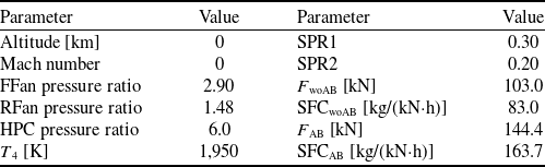
The design point parameters of the ACE are shown in Table 1. T ₄ denotes the turbine inlet temperature. First bypass split ratio (SPR1) and second bypass split ratio (SPR2) represent the split ratio of the first and the second bypass, respectively. F denotes the thrust. SFC denotes the specific fuel consumption. The subscripts woAB and AB denote the afterburner on and off, respectively. The total excess air coefficient $\alpha$ is set to 1.1 when the afterburner is in operation.

Table 1.

ACE design point parameters

Table 1 Long description

A table with two columns labeled Parameter and Value, and six rows each. Row 1: Altitude, 0 kilometers; Mach number, 0. Row 2: FFan pressure ratio, 2.90; RFan pressure ratio, 1.48. Row 3: HPC pressure ratio, 6.0; T 4, 1,950 Kelvin. Row 4: SPR1, 0.30; SPR2, 0.20. Row 5: F woAB, 103.0 kilonewtons; SFCwoAB, 83.0 kilograms per kilonewton-hour. Row 6: F AB, 144.4 kilonewtons; SFCAB, 163.7 kilograms per kilonewton-hour.

The operating point of each component and the engine performance are calculated by the Newton–Raphson iterative method. The low-pressure shaft physical speed N _L is chosen as the engine’s main control variable.

To represent the variable geometry turbomachinery characteristics, multi-angle characteristic maps are adopted for the FFan, RFan, HPT and LPT. These maps are derived from the simulation data of variable geometry turbomachinery in the NASA Technical Reports [Reference Converse18–Reference Converse20], which are widely used in the ACE 0D simulation. The empirical relations to predict the maps with a changed IGV angle are used for the HPC [Reference Grönstedt14]. The constant-area mixer model [Reference Mattingly, Heiser and Pratt21] is used for the RVABI. Its variable geometry is realised by adjusting the bypass area while maintaining a constant total area for the core and bypass. The installation effect simulation is also incorporated with the 0D ACE model, which mainly considers the external flow losses of the inlet and nozzle [Reference Simmons7, Reference Plencner and Snyder22, Reference Kowalski23].

2.2 1D turbomachinery mean-line simulation method

As an efficient and physics-based method, the 1D performance simulation method is very suitable for the rapid design, analysis and optimisation of the turbomachinery, and also suitable for coupling with the engine performance simulation, to quickly analyse the effects of the design parameters, variable geometry, inter-stage bleeding and blade cooling on the component and engine performance under the whole engine environment.

The 1D method adopted in this paper is the mean-line method, which has been experimentally validated in Refs [Reference Zou, Zheng, Liu, Lai and Wang15, Reference Song, Wang, Fan, Zheng and Feng24, Reference Wang, Song, Zou, Yang, Wen, Zhou, Feng and Zheng25] and demonstrated good predictive accuracy over a wide range of operating conditions. The 1D mean-line method is based on the assumptions of steady state, inviscid and adiabatic conditions, and does not consider the changes of aerodynamic parameters along the circumferential and radial directions. Instead, it characterises the blade row by the aerodynamic parameters along the mean streamline. The empirical models of the incidence angle, the deviation angle and the flow losses, derived from a large amount of cascade tests and high-fidelity simulations, are employed to account for the actual flow effects on the turbomachinery performance.

The 1D methods for the adaptive fan and LPT both consist of two parts: the inverse design module (design point mode) and the direct analysis module (off-design point mode). By combining the inverse design module with the direct analysis module, the mean-line geometry, meridional flow path geometry, as well as the characteristic maps at different speeds can be predicted reasonably and rapidly, as shown in Fig. 2.

Figure 2.

Calculation flowchart of the 1D mean-line method.

Figure 2 Long description

The flowchart illustrates the calculation process of the 1D mean-line method. It is divided into two main modules: the Inverse design module and the Direct analysis module. The process starts with inputting inlet boundary conditions and design specifications. In the Inverse design module, 1D design parameters are set, and empirical models for the angle, loss, etc., are selected. The 1D inverse design code is then run, outputting aerodynamic and geometric parameters. A decision point checks if the performance meets requirements. If not, parameters are updated and the process returns to setting 1D design parameters. If yes, the process moves to the Direct analysis module. In the Direct analysis module, inlet boundary conditions, inverse design output, N subscript L, and variable geometry are inputted. 1D analysis parameters are set, and empirical models for the angle, loss, etc., are selected. The 1D direct analysis code is run, outputting characteristic maps. Another decision point checks if the performance meets requirements. If not, parameters are updated and transferred back to the Inverse design module. If yes, the process ends.

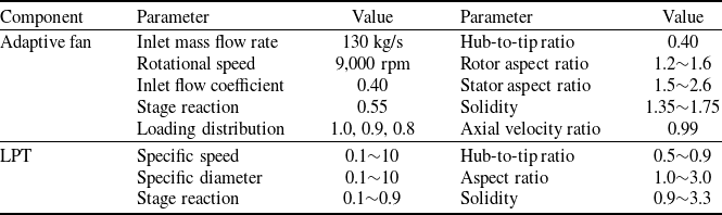
Table 2 presents the main design parameters of the adaptive fan and the LPT in the 1D simulation. The adaptive fan adopts a two-stage FFan and a single-stage RFan. A single-stage design is selected for the LPT. The selection of the adaptive fan parameters refers to the design parameters of the NASA highly loaded fan [Reference Messenger and Keenan26] and GE high-speed variable-geometry fan used in the variable cycle engine [Reference Sullivan and Parker19]. Besides, since an optimisation process is adopted in the 1D LPT inverse design, the ranges of optimisation variables and constraints are given in Table 2. The selection of the LPT parameters is based on the typical parameters used in the preliminary design and optimisation of axial-flow turbines, as described in Ref. [Reference Agromayor and Nord27].

2.3 0D–1D coupled ACE performance simulation method

To achieve the integration of the 0D engine model and the 1D component models, the iterative coupled approach was adopted. The iterative coupled approach progressively corrects the scaling factors of component characteristic maps in the 0D engine model based on discrepancies between the 0D engine model and 1D component models. This process iterates until the convergence criteria are satisfied, yielding consistent performance parameters for both components and the engine.

In this section, a 0D-1D iterative coupled simulation method is proposed by coupling the 1D mean-line models of the adaptive fan and the LPT with the 0D ACE model. The data is transferred bi-directionally between the 1D models and the 0D model through an iterative process. When the iteration is completed, all parameters at the engine level and the component level converge.

Table 2.

Design parameters of adaptive fan and LPT in 1D simulation

Table 2 Long description

A table comparing design parameters of adaptive fan and LPT in 1D simulation. The table has two main components: Adaptive fan and LPT, each with multiple parameters and their respective values. The Adaptive fan section includes parameters such as Inlet mass flow rate, Rotational speed, Inlet flow coefficient, Stage reaction, Loading distribution, Hub-to-tip ratio, Rotor aspect ratio, Stator aspect ratio, and Solidity. The LPT section includes parameters such as Specific speed, Specific diameter, Stage reaction, Hub-to-tip ratio, Aspect ratio, and Solidity. Each parameter has a corresponding value or range of values. For example, the Inlet mass flow rate for the Adaptive fan is 130 kilograms per second, and the Rotational speed is 9000 revolutions per minute. The LPT parameters are given in ranges, such as Specific speed from 0.1 to 10, and Specific diameter from 0.1 to 10.

Figure 3.

0D-1D coupled ACE simulation schematic diagram.

Figure 3 shows the schematic diagram of the 0D-1D coupled simulation, which mainly includes the following steps:

1. (i) Run the 0D ACE model to obtain the 0D component performance, engine performance and the boundary conditions of the adaptive fan and LPT.

For the adaptive fan, the boundary conditions include the inlet total pressure P _tin, and total temperature T _tin, N _L, IGV angle variation dVIGV1 (for FFan) and dVIGV2 (for RFan) and SPR2. During the coupled simulation, the pressure ratio (PR) from the 0D simulation is equal to that from the 1D simulation, to uniquely determine the adaptive fan operating point in the 1D simulation.

For the LPT, the boundary conditions include P _tin, T _tin, N _L, stator angle variation dVG, fuel-air ratio (FAR) and cooling parameters. The expansion ratio (ER) from the 0D simulation is equal to that from the 1D simulation, to uniquely determine the LPT operating point in the 1D simulation.

1. (ii) Run the 1D models of the adaptive fan and LPT to obtain the 1D component performance.

2. (iii) Generate the residuals (Res) of the corrected mass flow rate (Wc) and the isentropic efficiency (η), based on the differences between the 0D and 1D component performance, as shown in Equation (1).

   (1) \begin{align} {\mathop{\rm Re}\nolimits} {{\rm{s}}_p} = {{\left| {{p_{{\rm{1D}}}} - {p_{{\rm{0D}}}}} \right|}/{{p_{{\rm{0D}}}}}}\end{align}
   where the subscripts 0D and 1D denote the parameters calculated by the 0D model and 1D models, respectively. p denotes W _c or $\eta$ .

3. (iv) Update the scaling factors f for the generic characteristic maps of the FFan, RFan and LPT in the 0D model, which can be calculated by Equation (2).

   (2) \begin{align} {f_{p,i}} = \left[ {\left( {{{{p_{{\rm{1D}}}}} \over {{p_{{\rm{0D}}}}}} - 1} \right) \cdot \delta + 1} \right] \cdot {f_{p,i - 1}}\end{align}
   where i-1 and i represent the previous and the current iteration steps, respectively. $\delta$ indicates the relaxing factor. The relaxing factor governs the rate of change from the old value to the newly calculated one. A value closer to 1 implies faster updates and potentially quicker convergence, but may risk instability or oscillation. A smaller value (closer to 0) promotes stability by dampening changes but slows down convergence.

4. (v) Repeat the abovementioned steps until the convergence criterion is met.

5. (vi) Output the component performance and engine performance.

The residuals of different performance parameters govern the convergence of the 0D-1D coupled iteration. When the convergence residual changed from 1 × 10⁻³ to 1 × 10⁻⁴, the maximum performance variation was less than 0.03%. Therefore, a convergence residual of 1 × 10⁻³ was selected to balance the simulation accuracy with the computational cost. The relaxing factor for updating the component performance parameters between iterations is set to 0.8. This value was selected based on a sensitivity analysis conducted during the preliminary model development stage, where values ranging from 0.4 to 1.0 were tested. A factor of 0.8 was found to provide the best compromise between stability (avoiding oscillation) and convergence speed. Besides, through sufficient computational practices, it was found that the iteration number would not exceed 10. To allow for some margin, the maximum number of iterations was set to 20. These settings have been validated by confirming that the final converged solution is independent of the initial guesses within a practical range.

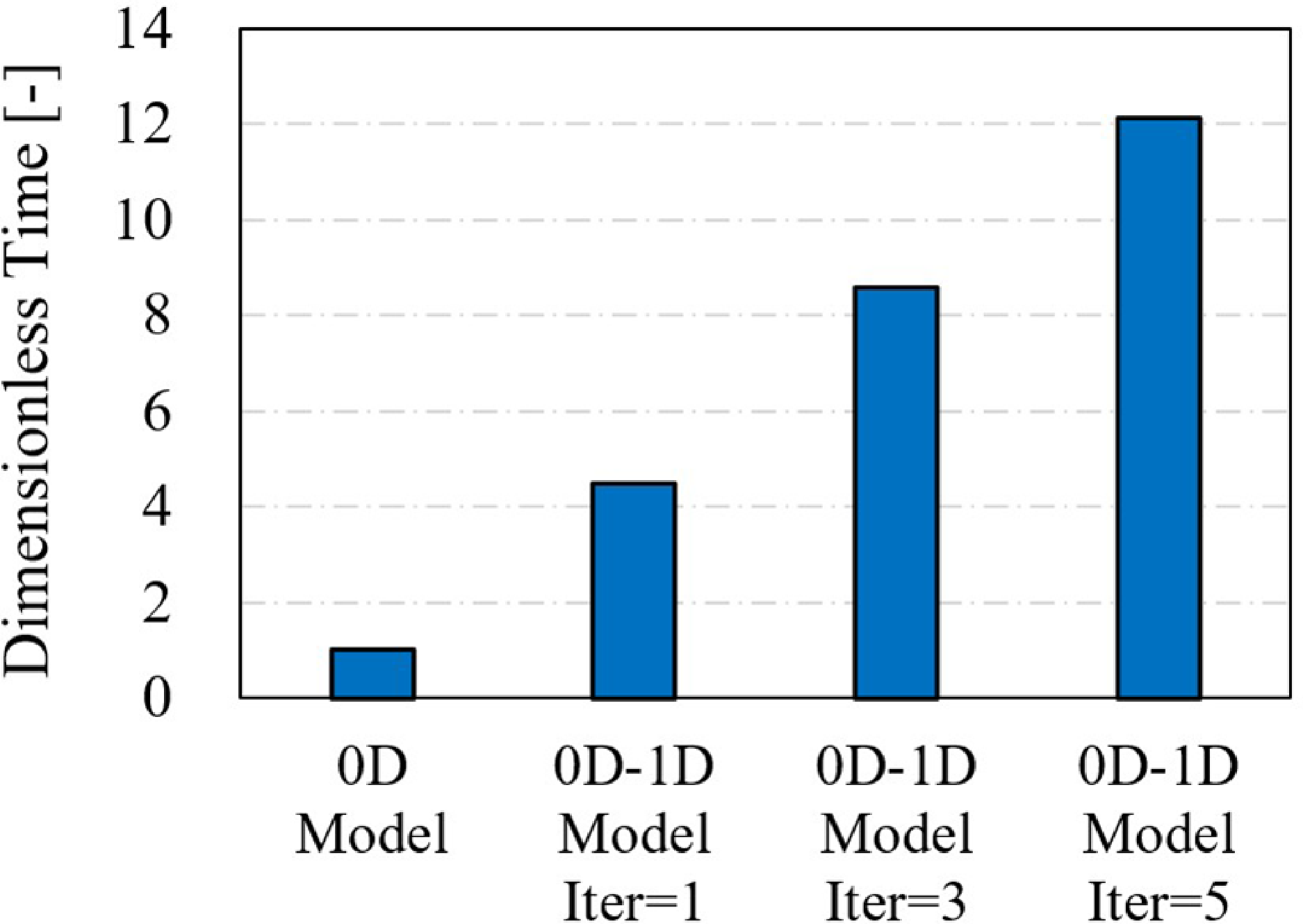
The comparison of computing time between the 0D-1D model and the 0D model is shown in Fig. 4. Iter indicates the iteration number in the 0D-1D coupled simulation. Compared with the 0D model, the 0D-1D model takes more computing time due to the run of the 1D model and the iterative process. Considering that the maximum number of iterations for a single point with the 0D-1D model does not exceed 10 in practice, the corresponding computing time is less than 1.5 min, which is acceptable during the conceptual design and preliminary design stages.

Figure 4.

Comparison of computing time between 0D-1D model and 0D model.

2.4 Optimisation method

Although ACE alleviates the performance compromise under different operating conditions by the operating mode adjustment, it is inevitable to adopt the optimisation methods to explore the ACE performance potential due to its more complex engine configuration, design space and control variables.

The ACE performance under different operating conditions is not only affected by the variable geometry parameters but also closely related to the design parameters. Therefore, the design parameters, the variable geometry parameters and the N _L are all selected as optimisation variables.

For the 0D model optimisation, the optimisation variables at design point include T ₄, SPR1, SPR2, the FFan pressure ratio PR_FFan, the RFan pressure ratio PR_RFan and the HPC pressure ratio PR_HPC. For the 0D-1D model optimisation, the optimisation variables at design point include T ₄, SPR1, SPR2, the adaptive fan pressure ratio PR_Fan, the stage load variation dPSI1 and dPSI2 and PR_HPC. dPSI1 and dPSI2 denote the stage load variation of the FFan second stage and the RFan relative to the previous stage, respectively. Different dPSI1 and dPSI2 indicate different distributions of pressure ratio between the FFan and RFan.

In both the 0D model and 0D-1D model optimisation, the variable geometry optimisation variables include the inlet guide vane angle (dVG) of the FFan, RFan, HPC and LPT, the RVABI bypass area variation dA _VABI, the variation of the core nozzle throat area dA8 and the variation of the bypass nozzle throat area dA18. The above parameters, together with N _L, are the optimisation variables at off-design point.

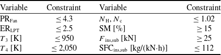
The optimisation constraints that consider the engine design requirements and engineering feasibility are shown in Table 3. At design point, the PR_Fan and the LPT expansion ratio ER_LPT do not exceed 4.3 and 2.5, respectively, to satisfy the performance requirements of the three-stage design and the single-stage design. Within the engine operating envelope, overtemperature, overspeed and surge must be avoided. T ₃ denotes the HPC outlet total temperature. N _H denotes the high-pressure shaft physical speed. N _c denotes the relative corrected speed. SM denotes the stall margin. The subscripts sub and ins denote the subsonic cruise condition and the installed performance, respectively.

Table 3.

Optimisation constraint

Table 3 Long description

The table has six rows and four columns. The columns are labeled Variable, Constraint, Variable, and Constraint. The rows list the following data: Row 1: PRFan, 4.3, N H, N c, 1.02. Row 2: ERLPT, 2.5, SM [%], 15. Row 3: T 3 [K], 950, F ins,sub [kN], 25. Row 4: T 4 [K], 2,050, SFCins,sub [kg/(kNh)], 112.

At take-off condition, the engine is required to provide the maximum thrust to take off as soon as possible, so maximising the thrust is set as the optimisation objective. At the cruise condition, the engine is required to reduce the SFC as much as possible to improve the fuel efficiency while achieving the minimum thrust, so minimising the installed SFC is taken as the optimisation objective.

NSGA-II uses the fast non-dominated sorting algorithm, elitist strategy and crowding distance parameter, which is a widely used multi-objective optimisation algorithm today. Based on the multi-objective optimisation platform PlatEMO [Reference Tian, Cheng, Zhang and Jin28], the NSGA-II algorithm [Reference Deb, Pratap, Agarwal and Meyarivan29] is adopted for the ACE performance optimisation to obtain the Pareto-optimal solutions. In this paper, the population size is set to 150. The maximum number of generations is set to 100. The crossover probability and mutation probability are set to 0.9 and 1/n, respectively (where n is the number of optimisation variables).

Surrogate modelling has attracted increased attention from researchers in various fields of engineering, which statistically relates input data to output data in complicated and computationally expensive system simulations. The common surrogate models involve the Kriging model, response surface model and neural network model. The main idea of the surrogate-based optimisation (SBO) is to obtain the samples based on the original physical model or high-fidelity model at first, and then build a surrogate model with high accuracy to replace the original model to carry out the optimisation [Reference Sun and Wang30, Reference Tao, Wang, Ye, Wang, Luo and Cui31]. SBO can avoid repeated calls to the physical model or high-fidelity model during the optimisation. Besides, the changes in the optimisation variables, constraints, objectives and algorithms can be flexibly considered without a large increase in computing cost and time, which significantly improves the optimisation efficiency. Considering the multiple input variables and strong nonlinear characteristics of the ACE optimisation, a BPNN-based optimisation strategy is proposed for the ACE optimisation. Figure 5 shows the BPNN-based optimisation flowchart.

Figure 5.

BPNN-based optimisation flowchart.

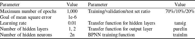
The ACE performance samples are obtained by the Latin hypercube sampling (LHS). The BPNN models are established based on the Neural Network Toolbox in MATLAB. The BPNN model accuracy is judged by the coefficient of determination R ². The BPNN model setting is shown in Table 4.

3.1 Parametric study at design point

At the take-off condition (design point), the effects of the design parameters on the ACE performance with and without afterburner operation are presented in Figs. 6 and 7, respectively. In Fig. 6, PR_t denotes the total pressure ratio. The arrow direction indicates the direction of parameter increase. In Fig. 7, the variations of the design parameters are as follows: T ₄ from 1950 K to 1750 K, SPR1 from 0.3 to 0.2, SPR2 from 0.2 to 0.3, PR_FFan from 2.9 to 3.2, PR_RFan from 1.5 to 1.7 and PR_HPC from 6.0 to 7.0.

Table 4.

BPNN model setting

Table 4 Long description

A table with two columns and eight rows, listing parameters and their values for a BPNN model. The first column lists the parameters: Maximum number of epochs, Goal of mean square error, Learning rate, Number of hidden layers, Number of hidden neurons, Training/validation/test set ratio, Transfer function for hidden layers, Transfer function for output layer, and BPNN training function. The second column lists the corresponding values: 1,000, 1e-6, 0.01, 1, 2, 70 percent/10 percent/20 percent, tansig, purelin, and trailm.

Figure 6.

Effects of design parameters on performance without afterburner operation (a) effects of PR_t and T₄ (b) effects of SPR1 and SPR2 (c) effects of PR_FFan and PR_RFan.

Figure 7.

Effects of design parameters on performance with afterburner operation (a) F_AB variation (b) SFC_AB variation (c) η variation.

When T ₄ decreases, F _woAB, F _AB and SFC_woAB decrease. However, with the afterburner operation, the temperature rises, and the fuel consumption in the afterburner increases, due to the constant $\alpha$ . The energy conversion rate in the afterburner is lower than that of the core combustor, increasing the SFC_AB.

When SPR1 decreases, more flow enters the core, leading to an increase in F _woAB and F _AB. Because the total bypass ratio BPR_t decreases, SFC_woAB increases. However, with the afterburner operation, SFC_AB decreases due to the constant αt and increased F _AB. When SPR2 increases, BPR_t increases, F _woAB, F _AB and SFC_woAB decrease. Because the total mass flow into the afterburner decreases, the total fuel flow decreases for the constant $\alpha$ , resulting in the decrease of SFC_AB.

When PR_FFan and PR_RFan increase, the PR_t increases, resulting in the decrease of SFC_woAB and SFC_AB and the increase of F _AB, but F _woAB changes a little. Increasing PR_HPC has a similar effect.

At design point, the main distinction between the 0D model and the 0D-1D model lies in whether the component efficiency changes with the pressure ratio or expansion ratio. Using the design parameters shown in Table 1, when the efficiency of FFan, RFan and LPT increases by 1.0%, F _woAB increases by 0.33, 0.12 and 0.22%, respectively, while SFC_woAB decreases by 0.15, 0.05 and 0.22%, respectively. As shown in Fig. 7, although the 0D model adopts the constant component efficiency while the 0D-1D model accounts for efficiency variations, the effect laws and magnitude of the design parameters from the two models are basically the same.

3.2 Parametric study at off-design point

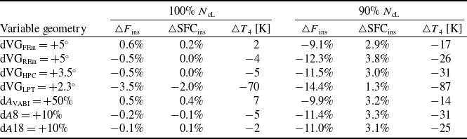
At the subsonic cruise condition, the effects of the variable parameters when the low-pressure corrected speed N _cL = 100% and N _cL = 90% are presented in Figs. 8 and 9, respectively. The effects of the variable geometry parameters on the component maps and operating points (OP) are shown in Fig. 10. The installed performance deviations after geometry variation are shown in Table 5. The positive dVG indicates the closing of the guide vane. Two models adopt the same empirical relation for the HPC variable geometry.

Figure 8.

Effects of variable geometry parameters on performance at 100% N_cL (a) F_woAB variation (b) SFC_woAB variation (c) T₄ variation.

Figure 9.

Effects of variable geometry parameters on performance at 90% N_cL (a) F_woAB variation (b) SFC_woAB variation (c) T₄ variation.

Figure 10.

Effects of variable geometry parameters on component maps and performance (a) effects of dVG_FFan (b) effects of dVG_RFan (c) effects of dVG_LPT.

The effects of the dVGFFan, dVGRFan and dVGLPT are highlighted below.

Turning down the FFan guide vane, the FFan mass flow rate and pressure ratio decrease, while the power consumption decreases, resulting in an increasing trend in N _L. To keep N _L constant, T ₄ decreases, and N _H also decreases. As a result, the core flow capacity decreases, and BPR_t increases. Finally, both F and SFC decrease. As the FFan guide vane closes, the pressure ratio characteristic shifts to the lower left, and the efficiency characteristic shifts to the left for both the 0D FFan map and the 1D FFan map. However, when N _L is reduced from 100 to 90%, the mass flow rate and pressure ratio in the 1D FFan map decrease more than those of the 0D map. Besides, the maximum efficiency of the 1D map tends to decrease, while the maximum efficiency of the 0D map tends to increase. This results in a significant increase in the performance deviation at N _cL = 90%, as shown in Table 5.

Turning down the RFan guide vane, the power consumption of RFan decreases. To keep N _L constant, T ₄ and N _H decrease. Due to the decreased flow capacity of the RFan and the core, BPR_t increases, and F and SFC decrease. Turning down the RFan guide vane has basically the same effect on the 0D RFan map and 1D RFan map. However, the RFan efficiency of the 0D model is about 2% higher than the 0D-1D model at N _cL = 90%.

Turning down the LPT guide vane, the HPT expansion ratio PR_HPT and the output work P _HPT decrease, and N _H decreases, decreasing the core flow capacity W _core, then increasing the BPR_t. It also has multiple and contradictory effects on the T ₄.

Table 5.

Performance deviations between 0D model and 0D-1D model after geometry variation

Table 5 Long description

A table with seven rows and six columns comparing performance deviations between 0D model and 0D-1D model after geometry variation. The columns are labeled as Variable geometry, ΔF_ins, ΔSFC_ins, ΔT4 [K] for 100% N_cL and 90% N_cL. The rows are labeled as dVG_FFan = +5°, dVG_RFan = +5°, dVG_HPC = +3.5°, dVG_LPT = +2.3°, dA_VAB1 = +50%, dA8 = +10%, dA18 = +10%. The values in the table are as follows: Row 1: dVG_FFan = +5°, 0.6 percent, 0.2 percent, 2 K, -9.1 percent, 2.9 percent, -17 K. Row 2: dVG_RFan = +5°, -0.5 percent, 0.0 percent, -4 K, -12.3 percent, 3.8 percent, -26 K. Row 3: dVG_HPC = +3.5°, -0.5 percent, 0.0 percent, -5 K, -11.5 percent, 3.0 percent, -31 K. Row 4: dVG_LPT = +2.3°, -3.5 percent, -2.0 percent, -70 K, -14.4 percent, 1.3 percent, -87 K. Row 5: dA_VAB1 = +50%, 0.5 percent, 0.4 percent, 7 K, -9.9 percent, 3.2 percent, -14 K. Row 6: dA8 = +10%, -0.2 percent, -0.1 percent, -5 K, -11.4 percent, 3.3 percent, -31 K. Row 7: dA18 = +10%, -0.1 percent, 0.1 percent, -2 K, -11.0 percent, 3.1 percent, -25 K.

The LPT expansion ratio PR_LPT increases, resulting in an increasing trend of N _L. To keep N _L constant, the fuel mass flow rate W _f should be reduced, resulting in a decreasing trend of T ₄.

The core flow capacity W _core decreases, resulting in a decreasing trend of the LPT output work P _LPT and N _L. To keep N _L constant, the fuel mass flow rate W _f should be increased, resulting in an increasing trend of T ₄.

Because W _core decreases, the back pressure of the FFan and RFan (Pb _FFan and Pb _RFan) increases, and the pressure ratio (PR_FFan and PR_RFan) and power consumption (P _FFan and P _RFan) increase, resulting in a decreasing trend of N _L. To keep N _L constant, T ₄ increases.

Besides, turning down the LPT guide vane will also affect the component efficiency. The increase (or decrease) in the component efficiency will result in an increasing (or decreasing) trend of N _L and a decreasing (or increasing) trend of T ₄.

Under the comprehensive influence of the above factors, T ₄ increases to keep N _L constant. The variations of F and SFC mainly depend on the combined effects of BPR_t and T ₄.

To further analyse the effects of LPT variable geometry, the effects of the LPT efficiency variation △ $\eta$ _LPT and the mass flow variation △W _cLPT on the ACE performance variation are shown in Fig. 12, which presents the possible variations of the LPT characteristic after turning down the LPT guide vane.

Figure 11.

Effects of increased dVG_LPT on N_L and T₄.

Figure 12.

Effects of increased dVG_LPT on performance (a) F_woAB variation (b) SFC_woAB variation (c) T₄ variation (d) BPR_t variation.

The variations of F and SFC are linear with △ $\eta$ _LPT, but are nonlinear with △W _cLPT. When different LPT variable geometry characteristics are adopted, the variations of F and SFC may be positive or negative, which means F and SFC may increase or decrease. When the △W _cLPT is small, the variation trends of F and SFC mainly depend on the △ $\eta$ _LPT. If the $\eta$ _LPT decreases, F and SFC increase due to higher T ₄ and lower BPR_t, corresponding to the 0D model results in Figs. 8 and 9. If the $\eta$ _LPT changes slightly or increases, F and SFC decrease, the former corresponding to the 0D-1D model results in Figs. 8 and 9. When the △W _cLPT is large, both F and SFC increase over a large range of △ $\eta$ _LPT.

With the constant N _L as the control law, studies in the literature [Reference Lyu, Tang and Chen32–Reference Xu, Tang and Chen34] showed that turning down the LPT guide vane would reduce T ₄, F and SFC, while the literature [Reference Zheng, Chen and Tang13, Reference Chen, Zhang and Tang35] drew an opposite conclusion. As shown in Figs. 8 and 9, turning down the LPT guide vane, T ₄, F and SFC obtained from the 0D model are increased. However, T ₄ from the 0D-1D model increases, but the increasing amplitude is significantly less than that from the 0D model, contributing to the decrease of F and SFC. The main reason is: after turning down the LPT guide vane, the LPT efficiency from the 0D-1D model is significantly higher (3.5∼4.5% higher). Besides, the LPT mass flow rate is also larger, which means the larger HPT expansion ratio (about 4.5% higher), the larger N _H and the larger core flow capacity from the 0D-1D model. The above factors result in a lower T ₄ compared with the 0D model. Under such circumstances, F and SFC decrease in the 0D-1D model as a result of the lower T ₄ and higher BPR_t.

In summary, the differences in the component characteristics with variable geometry between the two models make an important impact on the ACE performance, especially when the operating point deviates from the design condition. Particularly, accurate prediction of the mass flow and efficiency characteristics of the variable geometry LPT is critical to the ACE performance prediction. When the variable geometry LPT characteristics deviate significantly from the true values, the performance trends predicted by the 0D model may be opposite to reality.

4.1 Determination of optimisation variable range

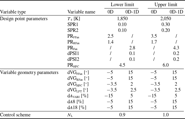
The optimisation variable ranges are shown in Table 6. The design point parameters are specified based on the available literature data and engineering experience. Since the variable geometry parameters work only at the subsonic cruise condition in the optimisation, the adjustment direction of the variable geometry parameters is mainly determined according to the decreasing direction of the SFC. As shown in Fig. 8, the guide vane of FFan and RFan should be turned down (increased dVG), the HPC guide vane should be opened (decreased dVG), the dA _VABI should be decreased and dA8 should be increased. The dVG_HPC ranges from −3.5° to 2°, which corresponds to the range of the mass flow factor from 115 to 95% [Reference Grönstedt14]. As described in Section 3.2, the effects of variable geometry LPT on engine performance are multifaceted, and its impact on the SFC is not monotonous, which is highly correlated with the mass flow variation of the LPT. Therefore, in this paper, the range of dVG_LPT is determined based on the requirements of the mass flow variation. For variable geometry LPT, a typical range of the mass flow variation is from 110 to 90%, corresponding to a dVG_LPT range of approximately −3.5° to 2.5° [Reference Converse20].

Table 6.

Optimisation variable ranges

Table 6 Long description

The table has three main sections: Design point parameters, Variable geometry parameters, and Control scheme. Each section lists variable names, lower limits, and upper limits for 0D and 0D-1D. Design point parameters include variables like T4 [K], SPR1, SPR2, PRFFan, PRRFan, PRFan, dPSI1, dPSI2, and PRHPC. Variable geometry parameters include dVGFFan, dVGRFan, dVGHPC, dVGLPT, dAVABI, dA8, and dA18. The Control scheme section lists NL. Each variable has specified lower and upper limits for 0D and 0D-1D. The table provides a detailed comparison of these ranges.

4.2 BPNN prediction model establishment

According to the optimisation variable ranges in Table 6, the LHS is adopted to obtain the ACE performance samples, and then the BPNN model for every engine performance parameter can be established based on the samples. The selection of BPNN hyperparameters, including the sample size (SZ), the number of hidden layers (HLN) and the number of hidden layer neurons (HLNN), is guided by the parametric study.

The effects of the BPNN hyperparameters on the R ² of the SFC_sub in the 0D-1D model are presented in Fig. 13. The model accuracy metrics tend to stabilise when the training set SZ approaches approximately 4,000, indicating that further increasing the samples will not result in a significant improvement in accuracy. Therefore, SZ = 4,000 is selected to ensure the surrogate model accuracy while maintaining a manageable computational cost for data generation. As the HLNN increases, the R ² on the training set increases when HLN = 1, while it increases first and then decreases when HLN = 2. Besides, the complex network architecture weakens the generalisation ability of the BPNN model. Therefore, with the increase of HLNN, the R ² on the test set tends to increase first and then decrease. Based on the parametric study results on the BPNN hyperparameters, SZ = 4,000, HLN = 2 and HLNN = 16 are ultimately selected, as they provide an optimal balance between high accuracy (both for training set and test set) and model robustness against overfitting.

Figure 13.

Effects of BPNN model hyperparameters on R² of SFC_sub in 0D-1D model (a) HLN = 1 (b) HLN = 2.

With the above setup, the performance comparisons between the 0D-1D model and the BPNN model in the test set are shown in Fig. 14. The R ² and mean absolute error (MAE) of each performance parameter in the test set are shown in Table 7. The R ² of F, SFC and T ₄ are larger than 0.997, 0.972 and 0.970, respectively, indicating that the established BPNN models have sufficient prediction accuracy for the ACE performance.

Figure 14.

Performance comparisons between the 0D-1D model and BPNN model in the test set (a) F_TO (b) W_f,TO (c) F_sub (d) W_f,sub.

4.3 Optimisation results and analysis

BPNN-based multi-objective performance optimisation is carried out towards two critical operating conditions, which can be described as follows:

1. 1) Optimisation objectives: the take-off thrust F _TO is maximised and the subsonic cruise specific fuel consumption SFC_sub is minimised, simultaneously.

2. 2) Optimisation variables: the design parameters X _des and the off-design parameters X _offdes are selected (the latter include the variable geometry parameters and control scheme), as detailed in Table 6.

3. 3) Optimisation constraints: the optimisation is subject to the engine performance and operational limits specified in Table 3, including the temperature limit, rotational speed limit, surge margin requirement and other key parameters.

The optimisation problem is defined in Equation (3).

(3) \begin{align} & \left\{\begin{array}{l} \textrm{max}\;F_{\textrm{To}} = f_{\textrm{TO}}(X_{\textrm{des}}) \\\textrm{min}\;\textrm{SFC}_{\textrm{sub}} = f_{\textrm{sub}}(X_{\textrm{des}},X_{\textrm{offdes}}) \end{array} \right. \nonumber \\& s.t. \quad X_{\textrm{des,low}} \leq X_{\textrm{des}} \leq X_{\textrm{des,up}},X_{\textrm{offdes,low}} \leq X_{\textrm{offdes}} \leq X_{\textrm{offdes,up}}\nonumber \\&\qquad \{PR_{\textrm{Fan}},ER_{\textrm{LPT}},T_{3},T_{4},N_{\textrm{H}},N_{\textrm{c,FFan}},N_{\textrm{c,RFan}},N_{\textrm{c,HPC}},SFC_{\textrm{sub}}\} \leq C_{\textrm{up}}\nonumber \\&\qquad \{SM_{\textrm{FFan}},SM_{\textrm{RFan}},SM_{\textrm{HPC}},F_{\textrm{TO}},F_{\textrm{sub}}\}\geq C_{\textrm{low}} \end{align}

where f _TO denotes the mapping relation between the optimisation variables at the design point X _des and F _TO established by the BPNN model. f _sub denotes the mapping relation between the X _des, the optimisation variables at off-design point X _offdes and SFC_sub. C denotes the optimisation constraints. The subscripts low and up indicate the lower limit and upper limit, respectively.

Table 7.

R² and MAE in the test set

Table 7 Long description

A table comparing performance metrics of different models. The table has 2 rows and 10 columns. The columns are labeled as Model Type, F_TO R^2, F_TO MAE, SFC_TO R^2, SFC_TO MAE, F_sub R^2, F_sub MAE, SFC_sub R^2, SFC_sub MAE, and T_4_sub R^2, T_4_sub MAE. The row labels are 0D and 0D-1D. Row 1: 0D, 0.998, 0.207, 0.995, 0.237, 0.997, 0.254, 0.987, 0.419, 0.991, 12.76. Row 2: 0D-1D, 0.999, 0.159, 0.999, 0.185, 0.997, 0.344, 0.972, 0.647, 0.970, 22.33.

Figure 15.

Comparison of Pareto front from multi-objective optimisation.

The Pareto fronts obtained by the optimisation are shown in Fig. 15. The optimal solutions of both models exhibit a typical trade-off relationship. On the Pareto front, the greater the sea-level thrust F _TO, the higher the subsonic cruise fuel consumption SFC_sub. The Pareto front from the 0D-1D model is located at the lower right side of that from the 0D model, which indicates that the engine performance from the 0D-1D model is superior. Moreover, in the region of the smaller F _TO and the lower SFC_sub, the difference between the Pareto fronts of the two models is even larger.

The comparisons of F _sub, SFC_sub and T _4,sub during multi-objective optimisation are shown in Fig. 16. The Pareto solutions are also illustrated in the figure. The F _sub is overall positively correlated with T _4,sub. The dispersion is mainly due to the differences in the bypass ratio and the component characteristics. The SFC_sub and F _sub in Pareto solutions also show a generally positive correlation. The performance dispersion of the 0D-1D Pareto solutions is greater than that of the 0D Pareto solutions, mainly because the component characteristics of the 0D-1D model change more significantly than those of the 0D model during the optimisation. The 0D model employs constant component efficiency at design point and multi-angle generic maps to represent the component characteristics. By contrast, the 0D-1D model adopts the physics-based 1D models to predict component characteristics, which enables a more accurate evaluation of the influence of design parameters and variable geometry parameters on the component characteristics. Consequently, at each optimisation point, the 0D-1D model exhibits greater variation in component characteristics compared to the 0D model.

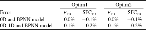
The solutions Optim1 (F _TO = 150 kN) and Optim2 (F _TO = 159 kN) in Fig. 15 are selected for comparison. The performance errors between the 0D/0D-1D model and the BPNN model in Optim1 and Optim2 are shown in Table 8. The errors of both F _TO and SFC_sub are within 0.2%, which demonstrates the sufficient accuracy of the BPNN model and the BPNN-based optimisation method.

Figure 16.

Comparison of engine performance during multi-objective optimisation (a) scatter plot of F_sub and T_4,sub (b) scatter plot of F_sub and SFC_sub.

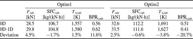
The comparisons of the subsonic performance between the two models under the solution Optim1 and Optim2 are shown in Table 9. The SFC_sub from the 0D-1D model is 1.7 and 0.6% lower than that from the 0D model in the solution Optim1 and Optim2, respectively, while the F _sub from the 0D-1D model is 4.5 and 2.5% higher, respectively.

The comparisons of the optimisation variables and the component efficiency between the two models are shown in Figs. 17 and 18, respectively.

For Optim1, to achieve lower SFC_sub, both models adopt lower T ₄, higher SPR1, and higher total pressure ratio at design point, as shown in Fig. 17(a). Meanwhile, to balance the F _TO, a lower SPR2 design value is adopted, so that the BPR_t design value is not too large. High PR_FFan and low PR_RFan are adopted, and the design value of the adaptive fan pressure ratio reaches the upper limit of 4.3. Under subsonic cruise condition, both models turn down the RFan guide vane, decrease the dA_VABI, and increase the A8, to reduce the T ₄ and increase the BPR_t, thereby reducing the SFC_sub. The inlet guide vane angle of the HPC and the LPT is basically unadjusted in the 0D model, but turned down in the 0D-1D model. The FFan guide vane angle and A18 are adjusted in the opposite direction for both models. The above variable geometry scheme makes the BPR_t of the 0D-1D model higher. In addition, under subsonic cruise condition, the efficiency of the RFan, HPT and LPT from the 0D-1D model is higher, but the FFan efficiency is lower than that of the 0D model. The lower SFC_sub is achieved by the higher rotational speed, wider range of the variable geometry parameters and higher component efficiency for the 0D-1D model, while it is achieved by the lower rotational speed and the smaller geometry variation for the 0D model. Finally, the 0D-1D model obtains a lower SFC_sub than the 0D model, due to a higher T _4,sub (indicating a higher thermal efficiency) and higher BPR_t,sub (indicating a higher propulsive efficiency), as shown in Table 9.

Table 8.

Performance errors between 0D or 0D-1D model and BPNN model

Table 8 Long description

A table comparing performance errors between 0D or 0D-1D model and BPNN model. The table has two columns labeled Optim1 and Optim2, each with sub-columns F_TO and SFC_TO. There are two rows labeled 0D and BPNN model, and 0D-1D and BPNN model. Row 1: Optim1 F_TO, 0.0 percent; Optim1 SFC_TO, minus 0.1 percent; Optim2 F_TO, 0.0 percent; Optim2 SFC_TO, minus 0.1 percent. Row 2: Optim1 F_TO, minus 0.1 percent; Optim1 SFC_TO, minus 0.2 percent; Optim2 F_TO, minus 0.1 percent; Optim2 SFC_TO, minus 0.2 percent.

Table 9.

Performance comparisons between 0D model and 0D-1D model under subsonic cruise condition

Table 9 Long description

The table compares performance metrics between 0D and 0D-1D models under subsonic cruise conditions for two optimization solutions, Optim1 and Optim2. It has two main sections, one for each optimization solution, each containing four columns: F_sub in kilonewtons (kN), SFC_sub in kilograms per kilonewton-hour (kg/(kN-h)), T_4sub in kelvins (K), and BPR_sub. Each section also includes a row for deviations. Panel A: For Optim1, the 0D model has F_sub of 28.5 kN, SFC_sub of 106.7 kg/(kN-h), T_4sub of 1,557 K, and BPR_sub of 0.56. The 0D-1D model has F_sub of 29.8 kN, SFC_sub of 104.8 kg/(kN-h), T_4sub of 1,580 K, and BPR_sub of 0.62. The deviations are 4.5 percent for F_sub, -1.7 percent for SFC_sub, 1.5 percent for T_4sub, and 11.6 percent for BPR_sub. Panel B: For Optim2, the 0D model has F_sub of 32.6 kN, SFC_sub of 112.2 kg/(kN-h), T_4sub of 1,691 K, and BPR_sub of 0.51. The 0D-1D model has F_sub of 33.5 kN, SFC_sub of 111.6 kg/(kN-h), T_4sub of 1,627 K, and BPR_sub of 0.41. The deviations are 2.5 percent for F_sub, -0.6 percent for SFC_sub, -3.8 percent for T_4sub, and -20.7 percent for BPR_sub.

Figure 17.

Comparison of optimisation variables between 0D model and 0D-1D model (a) Optim1 (b) Optim2.

For Optim2, although the difference in the SFC_sub and F _TO between the two models is not as large as that of Optim1, the difference in the optimisation variables between the two models is much larger, as shown in Fig. 17(b). In terms of the design parameters, the adaptive fan pressure ratio, HPC pressure ratio and SPR2 are essentially the same for both models. However, the 0D model achieves large F _TO through a design combination of high T ₄ and high SPR1, while the 0D-1D model adopts a design with lower T ₄ and lower SPR1. Moreover, since the design value of the T ₄ in the 0D-1D model has not yet reached the limit, the 0D-1D model can realise greater F _TO without the limitation of the SFC_sub. Under subsonic cruise condition, the analysis results of the variable geometry parameters are similar to Optim1. Due to the RFan guide vane being closed by 15° in the 0D model, the RFan efficiency in the 0D model is much lower than that of the 0D-1D model. Besides, the efficiency of the HPT and LPT from the 0D-1D model is higher, but the FFan efficiency is lower. Finally, the 0D-1D model also obtains a lower SFC_sub than the 0D model, as shown in Table 9.

Figure 18.

Comparison of component efficiency between 0D model and 0D-1D model under subsonic cruise condition (a) Optim1 (b) Optim2.

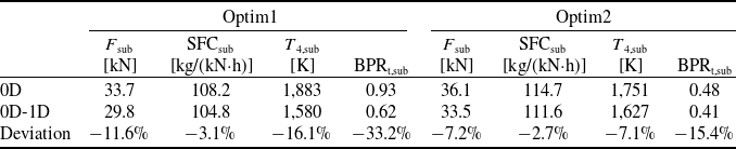
The comparisons of the subsonic performance between the 0D-1D model and the 0D model with the same optimisation variables are shown in Table 10. The 0D model adopts the same optimisation variables as the 0D-1D model in Optim1 or Optim2. The performance deviations between the two models are significantly larger than those in Table 9. By comparing Tables 10 and 9, it can be seen that for both Optim1 and Optim2, the T _4,sub of the 0D model increases significantly. This is mainly due to the increase in N _L under subsonic cruise condition (increasing from 0.907 to 0.964 for Optim1, and from 0.90 to 0.95 for Optim2). The increase in T _4,sub leads to an increase in F _sub and SFC_sub, thereby widening the performance gap between the 0D model and the 0D-1D model. The SFC_sub from the 0D-1D model is 3.1% and 2.7% lower than that from the 0D model in Optim1 and Optim2, respectively, and the F _sub from the 0D-1D model is 11.6% and 7.2% lower, respectively.