1 Introduction
The motion of particles in turbulence requires attention throughout disparate fields of engineering and the sciences. Some examples include transport of pollutant microplastics in ocean environments (Barboza & Gimenez Reference Barboza and Gimenez2015; Galloway, Cole & Lewis Reference Galloway, Cole and Lewis2017), pollen dispersion in atmospheric boundary layers (Hamaoui-Laguel et al. Reference Hamaoui-Laguel, Vautard, Liu, Solmon, Viovy, Khvorosthyanov, Essl, Chuine, Colette and Semenov2015), droplet and icy-crystal formation in clouds (Shaw Reference Shaw2003; Devenish et al. Reference Devenish, Bartello, Brenguier, Collins, Grabowski, Ijzermans, Malinowski, Reeks, Vassilicos and Wang2012), dispersion and deposition of firebrands (Anand, Shotorban & Mahalingam Reference Anand, Shotorban and Mahalingam2018) and potential jet engine failure caused by volcanic ash particles in the upper troposphere (Prata & Tupper Reference Prata and Tupper2009). The typical particles encountered in these examples of environmental concern are non-spherical and substantially smaller than the representative length scale of the flow field.
1.1 Background
Early work showed the motion of particles in turbulence in certain limiting cases, such as tracers (with no particle inertia) and small-but-massive highly inertial particles (Wang & Maxey Reference Wang and Maxey1993; Shin & Koch Reference Shin and Koch2005). Recent advances have shown the behaviour of particles in dynamical regimes between these limits. Some of the most intriguing results have focused on particles with non-spherical shape (Voth & Soldati Reference Voth and Soldati2017). Such shapes arise commonly in natural and engineering processes, including the examples mentioned above. Studies in homogeneous isotropic turbulence (HIT) have shown the important ways in which these non-spherical and moderately inertial particles vary relative to passive tracers (Parsa et al. Reference Parsa, Calzavarini, Toschi and Voth2012; Sabban, Cohen & van Hout Reference Sabban, Cohen and van Hout2017). A single elastic fibre was found to be slaved to the fluctuating velocity field in HIT (Rosti et al. Reference Rosti, Banaei, Brandt and Mazzino2018), thereby serving as a potential means to measure two-point statistics. These results represent a special case, however, because the lack of mean shear separates HIT from most of the turbulent flows found in practice. Herein, we approach the case of moderately inertial non-spherical particles in a turbulent channel flow.
Einarsson, Angilella & Mehlig (Reference Einarsson, Angilella and Mehlig2014) and Einarsson et al. (Reference Einarsson, Candelier, Lundell, Angilella and Mehlig2015) considered the effect of fluid and particle inertia on particles in simple shear. They showed that Jeffery orbits decay over time to the extreme cases of pure tumble or pure spin (also called ‘log rolling’). Subramanian & Koch (Reference Subramanian and Koch2005) provided a complementary study that considered the effect of stochastic perturbations (Brownian noise). Herein, we examine the case where perturbations are not random, but rather are those motions generated in a turbulent shear flow. We consider only particle inertia, and can justify this by studying the work of Lundell & Carlsson (Reference Lundell and Carlsson2010).
The turbulent channel flow presents an interesting case for particle motion because the flow changes between qualitatively different states with increasing distance from the channel wall. In the centre of the channel, the flow is essentially isotropic turbulence (Andersson, Zhao & Variano Reference Andersson, Zhao and Variano2015). Approaching the channel wall, mean shear breaks the isotropy. The effect of mean shear increases with proximity to the wall, until very close to the wall the flow is nearly the same as laminar simple shear. Laminar simple shear and isotropic turbulence cause very different types of particle motion (Lundell & Carlsson Reference Lundell and Carlsson2010; Parsa et al. Reference Parsa, Calzavarini, Toschi and Voth2012; Byron et al. Reference Byron, Einarsson, Gustavsson, Voth, Mehlig and Variano2015). For example, the magnitude of particle angular velocity is shape independent for isotropic turbulence but sensitive to shape for laminar simple shear. Another example is that inertial rod-shaped particles tend to rotate about their longest axis (‘spinning’) in isotropic turbulence, while shear flow causes them to rotate about their shortest axis (‘tumbling’). Such changes in particle behaviour are due to the fact that particle orientation and vorticity are orthogonal in simple shear flow and closely aligned in isotropic turbulence.
According to earlier findings in turbulent channel flow by Zhao et al. (Reference Zhao, Challabotla, Andersson and Variano2015), rods preferentially spin and disks tumble, just as in HIT, and particle inertia weakens this preference of rotation in the central region. Close to the channel walls, where the mean shear is dominant, both tumbling and spinning of tracers are suppressed with increasing asphericity. With increasing particle inertia, both disks and rods tend to rotate in the velocity-gradient plane, i.e. disks spin but rods tumble. The existence of two such qualitatively different modes of particle rotation, namely the ‘centre mode’ and the ‘wall mode’, has been documented in our recent studies (Zhao et al. Reference Zhao, Challabotla, Andersson and Variano2015; Zhao & Andersson Reference Zhao and Andersson2016; Yang, Zhao & Andersson Reference Yang, Zhao and Andersson2018). However, the fluid dynamical features of a turbulent channel flow vary considerably from the buffer region where the ‘wall mode’ prevails, to the channel centre, which resembles HIT, and where the ‘centre mode’ rotation is found. We aim to explore if another particle rotation mode exists in the relatively wide logarithmic layer. We also wish to demarcate the places where changes in particle rotation modes occur.
1.2 Eulerian–Lagrangian direct numerical simulations
Eulerian direct numerical simulation (DNS) coupled with a Lagrangian particle tracking approach has emerged as an effective tool for the study of particles in turbulence. In such Eulerian–Lagrangian (E-L) approaches, the carrying fluid flow field is treated as a continuum and solved on an Eulerian mesh whereas the solid particles are treated individually and subjected to Newton’s laws of motion. Different E-L methodologies can broadly be classified as point-particle direct numerical simulations (PP-DNSs) in which the particle mass centres are tracked in the fluid flow field and particle-resolved direct numerical simulations (PR-DNSs) in which the governing Navier–Stokes equations are solved with boundary conditions imposed on the surface of each finite-sized particle. A review of a broad variety of different simulation methods for suspensions of rigid particles was provided by Maxey (Reference Maxey2017).
1.2.1 PR-DNS
Particle-resolved DNSs involve computing of hydrodynamic forces and torques on the surface of each resolved particle, from which the particle’s velocity and position are advanced forward in time. The various methodologies use either body-fitted meshes for the integration of the Eulerian flow field to facilitate imposition of boundary conditions at the particle’s surface, or an immersed boundary (IB) method on a Cartesian mesh, as discussed in the review article by Tenneti & Subramaniam (Reference Tenneti and Subramaniam2014). The vast majority of particle-resolved DNSs, for instance those by Uhlmann (Reference Uhlmann2008) and Lucci, Ferrante & Elghobashi (Reference Lucci, Ferrante and Elghobashi2010), were concerned with finite-sized spherical particles typically of the order of the Taylor length scale
 $\unicode[STIX]{x1D6EC}$
. More recently, PR-DNSs were performed by Rosén, Lundell & Aidun (Reference Rosén, Lundell and Aidun2014), Do-Quang et al. (Reference Do-Quang, Amberg, Brethouwer and Johansson2014), Eshghinejadfard, Hosseini & Thévenin (Reference Eshghinejadfard, Hosseini and Thévenin2017) and Eshghinejadfard, Zhao & Thévenin (Reference Eshghinejadfard, Zhao and Thévenin2018) using lattice-Boltzmann methods (LBMs), whereas Ardekani et al. (Reference Ardekani, Costa, Breugem, Picano and Brandt2017a
) employed an IB method to simulate motion of non-spherical particles in viscous fluid flow. Rosén et al. (Reference Rosén, Lundell and Aidun2014), for instance, explored the competition between fluid inertia and particle inertia on the rotational dynamics of a single neutrally buoyant prolate spheroid in a laminar shear flow. Ardekani et al. (Reference Ardekani, Costa, Breugem, Picano and Brandt2017a
) were able to show that finite-sized oblate spheroids with aspect ratio
 $1:3$
could lead to drag reduction in turbulent channel flow.
Although the PR-DNS formalism is valid for particles of any size
 $\unicode[STIX]{x1D6FF}$
, conventional PR-DNS approaches are not feasible for particle sizes
 $\unicode[STIX]{x1D6FF}\ll \unicode[STIX]{x1D6EC}$
due to excessive computational demands. Unfortunately, many particles encountered in important applications are below this small-size limit, often with size
 $\unicode[STIX]{x1D6FF}$
comparable with the Kolmogorov length scale
 $\unicode[STIX]{x1D702}$
, i.e.
 $\unicode[STIX]{x1D6FF}\approx \unicode[STIX]{x1D702}$
. Motivated by this fact, Schneiders, Meinke & Schröder (Reference Schneiders, Meinke and Schröder2017a
,Reference Schneiders, Meinke and Schröder
b
) developed a novel approach to facilitate direct particle–fluid simulations (DPFS) of Kolmogorov-sized particles to extend the applicability of PR-DNS to smaller particles than usually studied by means of PR-DNS. The flow field over each particle is fully resolved by means of DNS of the momentum conservation equations, whereas the particle surfaces are discretely resolved using a Cartesian cut-cell method. Results from PR-DNSs of 45 000 spherical particles and prolate spheroids were reported by Schneiders et al. (Reference Schneiders, Meinke and Schröder2017a
) and Schneiders et al. (Reference Schneiders, Meinke and Schröder2017b
), respectively.
One decade ago Eaton (Reference Eaton2009) argued that computation of flow around hundreds of thousands of particles is beyond hope. Since all PR-DNS approaches require additional computational efforts compared to PP-DNSs, particle-resolved simulations are still limited to the order of 10 000 particles and becomes computationally too demanding for
 $\unicode[STIX]{x1D6FF}\lesssim \unicode[STIX]{x1D702}$
.
1.2.2 PP-DNS
Early point-particle simulations emerged several decades ago. Direct numerical simulations coupled with a Lagrangian point-particle tracking approach have proved to be an effective tool for the study of particles in turbulence; see for instance surveys by Eaton (Reference Eaton2009), Balachandar (Reference Balachandar2009), Balachandar & Eaton (Reference Balachandar and Eaton2010), Kuerten (Reference Kuerten2016) and Marchioli (Reference Marchioli, Minier and Pozorski2017). The point-particle approach requires the user to specify approximate equations for coupling the fluid and particle phases. This is in contrast to particle-resolved approaches that automatically include the volume occupied by the particles as well as the forces and torques coupling the two phases. Because of the need to specify simple equations to describe fluid–particle coupling, PP-DNSs cannot be justified for particles
 $\unicode[STIX]{x1D6FF}\geqslant \unicode[STIX]{x1D702}$
.
In one-way coupled PP-DNS only forces and torques from the fluid onto the individual point particles are considered, whereas the back reaction from the particles to the continuum phase is neglected. Marchioli & Soldati (Reference Marchioli and Soldati2002) and Sardina et al. (Reference Sardina, Schlatter, Brandt, Picano and Casciola2012) explored turbulence-induced wall accumulation of particles dispersed in wall turbulence (turbophoresis) as well as small-scale clustering in the form of local segregation that affects the particle distribution in the presence of fine-scale turbulence by means of one-way coupled PP-DNS. Sinking and sedimentation of phytoplankton in HIT, modelled as inertialess point spheroids, were investigated by Ardekani et al. (Reference Ardekani, Sardina, Brandt, Karp-Boss, Bearon and Variano2017b ).
When the back reaction from the particles on the fluid is accounted for (in two-way coupled simulations) modulation of the flow field by the particles can be studied. A straightforward point-force coupling was implemented by Rouson & Eaton (Reference Rouson and Eaton2001), but their computed results showed only negligible changes to the turbulence. The turbulence modulation depends intuitively on the particle loading and the two-way coupled PP-DNS by Zhao, Andersson & Gillissen (Reference Zhao, Andersson and Gillissen2010) showed that spherical particles suspended in a turbulent channel flow gave rise to drag reduction. An interesting assessment of the PP-DNS approach to non-spherical particles in decaying turbulence by comparison with PR-DNS results was presented by Frölich et al. (Reference Frölich, Schneiders, Meinke and Schröder2018).
A frequently overlooked fact is that the back reaction in the form of forces and possibly torques from the point particles utilize formulas, like those in equations (2.3) and (2.4), which involve information from the undisturbed flow field at the particle location. In two-way coupled simulations, the fluid velocity and velocity gradients are interpolated from a modulated flow field to the particle location since the undisturbed flow field is not available. Correction schemes to enable the undisturbed flow field to be deduced from the modulated flow field have recently been provided by Horwitz & Mani (Reference Horwitz and Mani2016), Ireland & Desjardins (Reference Ireland and Desjardins2017) and Balachandar, Liu & Lakhote (Reference Balachandar, Liu and Lakhote2019). The correction scheme proposed by Horwitz & Mani (Reference Horwitz and Mani2016) was validated by Horwitz & Mani (Reference Horwitz and Mani2018) and results obtained in decaying isotropic turbulence compared well with PR-DNS by Mehrabadi et al. (Reference Mehrabadi, Horwitz, Subramaniam and Mani2018). In one-way coupled PP-DNSs, such as the one presented herein, this challenge is not an issue since the only available flow field is the undisturbed flow field.
PP-DNSs were for a long time performed only for spherical particles. The first pioneering investigation of tiny prolate spheroids in directly simulated turbulent channel flow by an Eulerian–Lagrangian approach was conducted by Zhang et al. (Reference Zhang, Ahmadi, Fan and McLaughlin2001). The same approach was adopted by Mortensen et al. (Reference Mortensen, Andersson, Gillissen and Boersma2008a ), Marchioli, Fantoni & Soldati (Reference Marchioli, Fantoni and Soldati2010) and Zhao, Marchioli & Andersson (Reference Zhao, Marchioli and Andersson2014) focusing on effects of particle inertia and shape on particle concentrations, transport and rotation. Challabotla, Zhao & Andersson (Reference Challabotla, Zhao and Andersson2015b ,Reference Challabotla, Zhao and Andersson c , Reference Challabotla, Zhao and Andersson2016) carried out simulations of oblate spheroids and tracer tri-axial ellipsoidal particles in turbulent channel flow. Particle inertia drives oblate spheroids to orient in the flow-gradient plane in near-wall turbulence, similar to particle behaviour in simple shear flow (Challabotla, Nilsen & Andersson Reference Challabotla, Nilsen and Andersson2015a ). Zhao et al. (Reference Zhao, Challabotla, Andersson and Variano2015) took a first look into the rotational dynamics of prolate and oblate spheroids in two qualitatively different parts of the channel, i.e. in the centre and in the near-wall buffer layer. In these two regions of turbulent channel flow the particles behave with distinctly different rotation modes due to the presence or absence of wall shear; particle inertia adds complexity to the behaviour by changing the particle response time.
It is widely accepted that one-way coupled PP-DNS in the limits of (i) small particles and (ii) small volume fractions has a firm theoretical basis. Results from one-way coupled PP-DNS by Zhao et al. (Reference Zhao, Challabotla, Andersson and Variano2015) showed that inertia-free rods and disks in the core region of a turbulent channel flow were tumbling at the same rotation rates as measured in HIT by Parsa et al. (Reference Parsa, Calzavarini, Toschi and Voth2012) and Marcus et al. (Reference Marcus, Parsa, Kramel, Ni and Voth2014), respectively. The simulated tumbling rate was reduced by introduction of particle inertia (Zhao et al. Reference Zhao, Challabotla, Andersson and Variano2015) and this trend was confirmed by measurements reported by Sabban et al. (Reference Sabban, Cohen and van Hout2017) in their figure 18.
The present paper represents a sequel to the recent letter by Zhao et al. (Reference Zhao, Challabotla, Andersson and Variano2015), in which results were shown only in the buffer region and in the almost-isotropic channel centre. We now aim at a complete coverage of the particle dynamics across the entire channel, considering a wide range of particle shapes as well as a variety of different particle inertias. We explore the complete map of rotational behaviour, observing how behaviour transitions from outer to inner flow, i.e. from ‘centre mode’ to ‘wall mode’ rotation. We examine whether the qualitative regimes of particle behaviour change at locations that are already known to demarcate changes in qualitative fluid behaviour. We also examine how wide the region over which the rotation mode transitions is. We also examine interaction between outer and inner flow; for example, does the outer flow cause tracer particles to preferentially follow a subset of the infinite number of Jeffery orbits in the near-wall region? Finally, the answers to these questions can be compared for the cases of inertialess and inertial spheroids.
2 Mathematical modelling and methodology
The translational and rotational motion of rigid spheroidal particles in turbulent fluid flow is modelled in an Eulerian–Lagrangian approach, following the way paved by Zhang et al. (Reference Zhang, Ahmadi, Fan and McLaughlin2001), Mortensen et al. (Reference Mortensen, Andersson, Gillissen and Boersma2008a
,Reference Mortensen, Andersson, Gillissen and Boersma
b
), Marchioli et al. (Reference Marchioli, Fantoni and Soldati2010) and Zhao et al. (Reference Zhao, Marchioli and Andersson2014) for prolate spheroids and more recently by Challabotla et al. (Reference Challabotla, Zhao and Andersson2015c
) and Yuan et al. (Reference Yuan, Andersson, Zhao, Challabotla and Deng2017) for oblate spheroids. The inertial spheroids are considered as individual point particles obeying the laws of classical, i.e. Newtonian, mechanics. Multiple particles are suspended in a turbulent flow between two parallel walls, for which the turbulent flow field is obtained by means of a direct numerical simulation. The flow field is fully developed in space and statistically steady in time, validated by the observation that the mean velocity vector
 $\langle \boldsymbol{u}\rangle$
is aligned with the channel walls and all turbulence statistics are independent of the streamwise and cross-stream directions. The particle–fluid suspension is sufficiently dilute to justify one-way coupled simulations.
2.1 Lagrangian particle modelling
A spheroidal particle is characterized by three semi-axes
 $a=b\neq c$
. The aspect ratio
 $\unicode[STIX]{x1D706}=c/a$
distinguishes between prolate (
 $\unicode[STIX]{x1D706}>1$
) and oblate (
 $\unicode[STIX]{x1D706}<1$
) spheroids, whereas
 $\unicode[STIX]{x1D706}=1$
corresponds to an isotropic particle, i.e. a sphere. The motion of a spheroidal particle is described by using three different Cartesian coordinate systems: an inertial frame, a particle frame and a co-moving frame. The inertial frame,
 $\boldsymbol{x}=\langle x,y,z\rangle$
, spans the computational domain in which the fluid flow field is obtained by means of DNS. The particle frame,
 $\boldsymbol{x}^{\prime }=\langle x^{\prime },y^{\prime },z^{\prime }\rangle$
, is attached to the particle with its origin at the particle mass centre and the coordinate axes are aligned with the principal directions of particle inertia. The co-moving frame,
 $\boldsymbol{x}^{\prime \prime }=\langle x^{\prime \prime },y^{\prime \prime },z^{\prime \prime }\rangle$
, is also attached to the particle with its origin at the particle mass centre, but with the coordinate axes parallel to those of the inertial frame. The orientation of the particle’s axes relative to the co-moving frame is given by nine direction cosines (Goldstein Reference Goldstein1980), which relate the same vector in two different coordinate systems through the linear transformation
 $\boldsymbol{x}^{\prime }=\unicode[STIX]{x1D63C}\,\boldsymbol{x}^{\prime \prime }$
.
The translational and rotational motions of a single inertial spheroid with mass
 $m$
and moment of inertia
 $\unicode[STIX]{x1D644}$
obey
 $$\begin{eqnarray}\displaystyle \frac{\text{d}x_{i}}{\text{d}t}=v_{i};\quad m\frac{\text{d}v_{i}}{\text{d}t}=F_{i};\quad \unicode[STIX]{x1D610}_{ij}^{\prime }\frac{\text{d}\unicode[STIX]{x1D714}_{j}^{\prime }}{\text{d}t}+\unicode[STIX]{x1D716}_{ijk}\unicode[STIX]{x1D714}_{j}^{\prime }\unicode[STIX]{x1D610}_{kl}^{\prime }\unicode[STIX]{x1D714}_{l}^{\prime }=N_{i}^{\prime }, & & \displaystyle\end{eqnarray}$$
where
 $v_{i}$
denotes the translational particle velocity in the inertial frame, whereas
 $\unicode[STIX]{x1D714}_{i}^{\prime }$
is the angular velocity of the spheroid in the particle frame and
 $\unicode[STIX]{x1D716}_{ijk}$
is the Levi-Civita alternating tensor. It is particularly noteworthy that the translational motion of the spheroid is governed by Newton’s 2nd law of motion (2.1b
) expressed in the inertial reference frame, while the rotational motion is governed by Euler’s equation (2.1c
) formulated in the particle frame. The mass
 $m$
of a spheroidal particle with density
 $\unicode[STIX]{x1D70C}_{p}$
, i.e. an axisymmetric ellipsoid, and the diagonal elements of the moment of the inertia tensor
 $\unicode[STIX]{x1D610}_{ij}^{\prime }$
are
 $$\begin{eqnarray}\displaystyle m=\unicode[STIX]{x1D70C}_{p}\frac{4}{3}a^{3}\unicode[STIX]{x1D706};\quad \unicode[STIX]{x1D610}_{xx}^{\prime }=\unicode[STIX]{x1D610}_{yy}^{\prime }=\frac{(1+\unicode[STIX]{x1D706}^{2})ma^{2}}{5};\quad \unicode[STIX]{x1D610}_{zz}^{\prime }=\frac{2ma^{2}}{5}, & & \displaystyle\end{eqnarray}$$
whereas the off-diagonal elements of
 $\unicode[STIX]{x1D610}_{ij}^{\prime }$
are identically zero for spheroidal particles.
We assume that the spheroids are sufficiently small and that the neighbouring flow field can be considered as Stokesian. According to Brenner (Reference Brenner1964), the Stokesian hydrodynamic force
 $F_{i}$
acting on a spheroid from the surrounding fluid can be expressed as
 $$\begin{eqnarray}\displaystyle F_{i}=\unicode[STIX]{x03C0}a\unicode[STIX]{x1D707}\unicode[STIX]{x1D612}_{ij}(u_{j,p}-v_{j}). & & \displaystyle\end{eqnarray}$$
Here,
 $\unicode[STIX]{x1D707}$
is the dynamic viscosity of the fluid and the parenthetical term
 $\unicode[STIX]{x0394}u_{j}=u_{j,p}-v_{j}$
is the relative or slip velocity, i.e. the difference between the fluid velocity
 $u_{j,p}$
at the particle location and the particle velocity
 $v_{j}$
. The resistance tensor
 $\unicode[STIX]{x1D612}_{ij}$
in the inertial frame can be related to the constant and diagonal resistance tensor
 $\unicode[STIX]{x1D612}_{ij}^{\prime }$
in the particle frame through the transformation
 $\unicode[STIX]{x1D612}_{ij}=\unicode[STIX]{x1D608}_{ik}^{t}\unicode[STIX]{x1D612}_{kl}^{\prime }\unicode[STIX]{x1D608}_{lj}$
. Here,
 $\unicode[STIX]{x1D608}_{lj}$
are elements of the matrix
 $\unicode[STIX]{x1D63C}$
which transforms a vector from the co-moving frame to the particle frame. Analytical formulas for the diagonal elements of the resistance tensor
 $\unicode[STIX]{x1D612}_{ij}^{\prime }$
are provided in table 1.
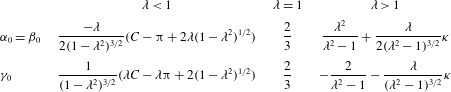
Elements of the diagonal resistance tensor
 $\unicode[STIX]{x1D612}_{ij}^{\prime }$
in the particle frame of reference for a spheroid with the
 $z^{\prime }$
-direction along the symmetry axis. The off-diagonal elements are all zero. The tensor elements for oblate and prolate spheroids are taken from Challabotla et al. (Reference Challabotla, Zhao and Andersson2015c
) and Gallily & Cohen (Reference Gallily and Cohen1979), respectively.
 $C=2\tan ^{-1}(\unicode[STIX]{x1D706}(1-\unicode[STIX]{x1D706}^{2})^{-1/2})$
is a shape-dependent constant.

The torque components
 $N_{i}^{\prime }$
acting on a three-axial ellipsoidal particle immersed in a creeping shear flow were originally derived by Jeffery (Reference Jeffery1922). For an axisymmetric particle with
 $z^{\prime }$
aligned with the particle’s symmetry axis, the expressions for the torque components become
 $$\begin{eqnarray}\displaystyle \left.\begin{array}{@{}l@{}}\displaystyle N_{x}^{\prime }=\frac{16\unicode[STIX]{x03C0}\unicode[STIX]{x1D707}a^{3}\unicode[STIX]{x1D706}}{3(\unicode[STIX]{x1D6FD}_{0}+\unicode[STIX]{x1D706}^{2}\unicode[STIX]{x1D6FE}_{0})}[(1-\unicode[STIX]{x1D706}^{2})\unicode[STIX]{x1D61A}_{yz}^{\prime }+(1+\unicode[STIX]{x1D706}^{2})(\unicode[STIX]{x1D6FA}_{x}^{\prime }-\unicode[STIX]{x1D714}_{x}^{\prime })]\\ \displaystyle N_{y}^{\prime }=\frac{16\unicode[STIX]{x03C0}\unicode[STIX]{x1D707}a^{3}\unicode[STIX]{x1D706}}{3(\unicode[STIX]{x1D6FC}_{0}+\unicode[STIX]{x1D706}^{2}\unicode[STIX]{x1D6FE}_{0})}[(\unicode[STIX]{x1D706}^{2}-1)\unicode[STIX]{x1D61A}_{xz}^{\prime }+(1+\unicode[STIX]{x1D706}^{2})(\unicode[STIX]{x1D6FA}_{y}^{\prime }-\unicode[STIX]{x1D714}_{y}^{\prime })]\\ \displaystyle N_{z}^{\prime }=\frac{32\unicode[STIX]{x03C0}\unicode[STIX]{x1D707}a^{3}\unicode[STIX]{x1D706}}{3(\unicode[STIX]{x1D6FC}_{0}+\unicode[STIX]{x1D6FD}_{0})}(\unicode[STIX]{x1D6FA}_{z}^{\prime }-\unicode[STIX]{x1D714}_{z}^{\prime }).\end{array}\right\} & & \displaystyle\end{eqnarray}$$
Here,
 $\unicode[STIX]{x1D61A}_{ij}^{\prime }$
and
 $\unicode[STIX]{x1D6FA}_{i}^{\prime }$
denote components of the local fluid rate-of-strain tensor and rate-of-rotation vector, respectively.
Dimensionless shape factors
 $\unicode[STIX]{x1D6FC}_{0}$
,
 $\unicode[STIX]{x1D6FD}_{0}$
and
 $\unicode[STIX]{x1D6FE}_{0}$
for spheroidal particles with aspect ratio
 $\unicode[STIX]{x1D706}$
. These analytical expressions for oblate and prolate spheroids were derived by Siewert et al. (Reference Siewert, Kunnen, Meinke and Schröder2014) and Gallily & Cohen (Reference Gallily and Cohen1979), respectively. The shape-dependent constants are defined as
 $C=2\tan ^{-1}(\unicode[STIX]{x1D706}(1-\unicode[STIX]{x1D706}^{2})^{-1/2})$
and
 $\unicode[STIX]{x1D705}=\ln [1-2(\unicode[STIX]{x1D706}^{2}-1)^{1/2}/(\unicode[STIX]{x1D706}+(\unicode[STIX]{x1D706}^{2}-1)^{1/2})]$
.

The expressions for the torque components in equation (2.4) are valid for any aspect ratio
 $\unicode[STIX]{x1D706}$
as long as the dimensionless shape factors
 $\unicode[STIX]{x1D6FC}_{0}$
,
 $\unicode[STIX]{x1D6FD}_{0}$
and
 $\unicode[STIX]{x1D6FE}_{0}$
are defined as semi-infinite integrals. Analytical expressions for the shape factors are provided in table 2 and have already been used to deduce the explicit expressions for the non-zero elements of the resistance tensor in table 1.
Finally, the time rate of change of the four Euler parameters is related to the particle angular velocity components in the following way:
 $$\begin{eqnarray}\displaystyle \left(\begin{array}{@{}c@{}}{\dot{e}}_{0}\\ {\dot{e}}_{1}\\ {\dot{e}}_{2}\\ {\dot{e}}_{3}\end{array}\right)=\frac{1}{2}\left(\begin{array}{@{}cccc@{}}e_{0} & -e_{1} & -e_{2} & -e_{3}\\ e_{1} & e_{0} & -e_{3} & e_{2}\\ e_{2} & e_{3} & e_{0} & -e_{1}\\ e_{3} & -e_{2} & e_{1} & e_{0}\end{array}\right)\left(\begin{array}{@{}c@{}}0\\ \unicode[STIX]{x1D714}_{x}^{\prime }\\ \unicode[STIX]{x1D714}_{y}^{\prime }\\ \unicode[STIX]{x1D714}_{z}^{\prime }\end{array}\right), & & \displaystyle\end{eqnarray}$$
where the dot denotes differentiation with respect to time. In addition, the time integration of the Euler parameters is subjected to the constraint
 $e_{0}^{2}+e_{1}^{2}+e_{2}^{2}+e_{3}^{2}=1$
.
The time evolution of a single inertial spheroid is governed by altogether eleven ordinary differential equations. The particle translational and rotational equations of motion (2.1b,c
) are discretized by means of a mixed differencing procedure (Fan & Ahmadi Reference Fan and Ahmadi1995) while equations (2.1a
) and (2.5) are solved by a second-order Adams–Bashforth scheme. A second-order quadratic interpolation scheme is used for interpolation of the flow variables at the particle positions, as required in equations (2.3) and (2.4). The numerical solution of these eleven particle equations is marched forward in time with the same time step
 $\unicode[STIX]{x0394}t$
as that used for the integration of the Navier–Stokes equations (see § 2.2).
The mechanical force
 $F_{i}$
and torque
 $N_{i}^{\prime }$
account for the impact from the viscous fluid in which the inertial spheroids are embedded. In the special case of the absence of inertia, however, an inertialess spheroid translates passively along with the fluid flow, i.e. the slip velocity
 $\unicode[STIX]{x0394}u_{j}=u_{j,p}-v_{j}=0$
. Equation (2.1b
) is no longer needed and we obtain the particle position from equation (2.1a
) with
 $v_{i}$
replaced by
 $u_{i,p}$
. Nevertheless, an inertialess spheroid exhibits a rotational motion different from the fluid rotation as long as
 $\unicode[STIX]{x1D706}\neq 1$
. Particle rotation in this limiting case is obtained by equating the Jeffery torque components
 $N_{i}^{\prime }$
to zero. Rotation of inertialess spheroids in wall turbulence has recently been explored by Challabotla et al. (Reference Challabotla, Zhao and Andersson2015b
), Zhao & Andersson (Reference Zhao and Andersson2016) and Yang et al. (Reference Yang, Zhao and Andersson2018). Herein, however, we focus on both inertial and tracer particles.
The particle suspensions considered are sufficiently dilute so that particle–particle collisions are rare and therefore of negligible importance. A particle is said to collide with the wall whenever the distance of the mass centre from the wall is smaller than the semi-axis
 $a$
. Particle–wall collisions are fully elastic so that a spheroid maintains its linear momentum in the wall-parallel plane as well as its angular momentum after a collision.
The point-particle approach can be justified as long as the size of the spheroids does not exceed the size of the smallest turbulent eddies, estimated by the Kolmogorov length scale
 $\unicode[STIX]{x1D702}$
. Similarly, Kolmogorov’s microscale for time
 $\unicode[STIX]{x1D70F}_{\unicode[STIX]{x1D702}}$
characterizes the motion of the very smallest turbulent eddies. The longest rods considered here have major axis
 $2c$
of the same order of magnitude as
 $\unicode[STIX]{x1D702}$
at all regions in the flow. Ravnik, Marchioli & Soldati (Reference Ravnik, Marchioli and Soldati2018) demonstrated that the Jeffery torques (2.4) nevertheless give a good representation of the torques acting on elongated particles. The assumption of Stokes flow in the immediate vicinity of a particle, on which the expressions for the force and torque components in (2.3) and (2.4) are based, can be justified provided that the particle Reynolds number based on the magnitude of the slip velocity
 $\unicode[STIX]{x0394}u_{i}$
is below 1. We check that this condition is satisfied during calculations. Corrections to the Stokesian equations may be needed, but these are generally not yet known for spheroids and are therefore omitted.
The ability of an inertial particle to adjust to the ambient flow field can be estimated in terms of a particle response time
 $\unicode[STIX]{x1D70F}_{p}$
. By means of the tensor elements in table 1, Shapiro & Goldenberg (Reference Shapiro and Goldenberg1993) derived a translational relaxation time for an isotropically oriented prolate spheroid, while Challabotla et al. (Reference Challabotla, Zhao and Andersson2015c
) deduced a response time for an isotropically oriented oblate spheroid,
 $$\begin{eqnarray}\displaystyle \unicode[STIX]{x1D70F}_{oblate}=\frac{\unicode[STIX]{x1D706}(\unicode[STIX]{x03C0}-C)}{2(1-\unicode[STIX]{x1D706}^{2})^{1/2}}\frac{2Da^{2}}{9\unicode[STIX]{x1D708}};\quad \unicode[STIX]{x1D70F}_{prolate}=\frac{2Da^{2}}{9\unicode[STIX]{x1D708}}\frac{\ln (\unicode[STIX]{x1D706}+(\unicode[STIX]{x1D706}^{2}-1)^{1/2})\unicode[STIX]{x1D706}}{(\unicode[STIX]{x1D706}^{2}-1)^{1/2}}, & & \displaystyle\end{eqnarray}$$
where
 $D=\unicode[STIX]{x1D70C}_{p}/\unicode[STIX]{x1D70C}_{f}$
is the ratio between particle and fluid densities and the shape-dependent constants
 $C$
and
 $\unicode[STIX]{x1D705}$
are defined in the caption of table 2.
2.2 Fluid phase modelling
The motion of the continuous Newtonian fluid phase, in which the point spheroids are suspended, is governed by continuity and Navier–Stokes equations. For incompressible flow, these equations are non-dimensionalized as
 $$\begin{eqnarray}\displaystyle \frac{\unicode[STIX]{x2202}u_{i}}{\unicode[STIX]{x2202}x_{i}}=0,\quad \frac{\unicode[STIX]{x2202}u_{i}}{\unicode[STIX]{x2202}t}+u_{j}\frac{\unicode[STIX]{x2202}u_{i}}{\unicode[STIX]{x2202}x_{j}}=-\frac{\unicode[STIX]{x2202}p}{\unicode[STIX]{x2202}x_{i}}+\frac{1}{Re_{\unicode[STIX]{x1D70F}}}\frac{\unicode[STIX]{x2202}^{2}u_{i}}{\unicode[STIX]{x2202}x_{j}\unicode[STIX]{x2202}x_{j}}. & & \displaystyle\end{eqnarray}$$
Here,
 $u_{i}$
and
 $x_{i}$
are the
 $i$
th components of the velocity and position vectors, normalized by the velocity scale
 $u_{\unicode[STIX]{x1D70F}}$
and the length scale
 $h$
, respectively, and
 $Re_{\unicode[STIX]{x1D70F}}=u_{\unicode[STIX]{x1D70F}}h/\unicode[STIX]{x1D708}$
is the Reynolds number. Although the fluid phase is to be loaded with inertial particles, the resulting suspension is sufficiently dilute so that a one-way coupled simulation can be justified and no reaction force from the particles is included in equation (2.7b
).
We simulate a fully developed turbulent channel flow at Reynolds number
 $Re_{\unicode[STIX]{x1D70F}}=180$
. The DNS solver used to integrate the governing equations (2.7) is the same as that employed by Gillissen et al. (Reference Gillissen, Boersma, Mortensen and Andersson2007) and Mortensen et al. (Reference Mortensen, Andersson, Gillissen and Boersma2008a
,Reference Mortensen, Andersson, Gillissen and Boersma
b
). A constant mean pressure gradient
 $\text{d}P/\text{d}x<0$
is added to
 $-\unicode[STIX]{x2202}p/\unicode[STIX]{x2202}x_{i}$
in order to drive the viscous fluid through the channel in the positive
 $x$
-direction, i.e. between two parallel walls a distance
 $2h$
apart. The wall friction velocity
 $u_{\unicode[STIX]{x1D70F}}$
, which is adopted as the velocity scale, becomes
 $u_{\unicode[STIX]{x1D70F}}=\sqrt{h|\text{d}P/\text{d}x|/\unicode[STIX]{x1D70C}}$
. Periodic boundary conditions are used in the homogeneous streamwise (
 $x$
) and cross-stream (
 $y$
) directions, whereas no-slip and impermeability conditions are imposed at the two channel walls.
The size of the computational domain used is
 $12h\times 6h\times 2h$
and discretized with
 $192^{3}$
grid points. This gives the grid resolution
 $\unicode[STIX]{x0394}x^{+}=11.3$
and
 $\unicode[STIX]{x0394}y^{+}=5.6$
in the streamwise and cross-stream directions, respectively, where the superscript
 $+$
indicates normalization with viscous units. The grid in the wall-normal direction is refined near the walls such that
 $\unicode[STIX]{x0394}z^{+}$
varies between 0.9 and 2.86. The dimensionless time step used is
 $\unicode[STIX]{x0394}t^{+}=\unicode[STIX]{x0394}tu_{\unicode[STIX]{x1D70F}}^{2}/\unicode[STIX]{x1D708}=0.036$
.
2.3 Turbulent channel flow
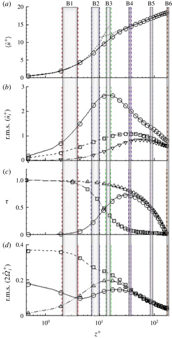
The most relevant flow statistics are presented in figure 1, which shows how the essential flow variables vary from the channel wall at
 $z^{+}=0$
to the channel mid-plane at
 $z^{+}=180$
. These statistics vary symmetrically about the channel centre, except the shear stresses in figure 1(c) which vary anti-symmetrically about the mid-plane. The perfect agreement with the DNS data of Moser, Kim & Mansour (Reference Moser, Kim and Mansour1999) obtained at
 $Re_{\unicode[STIX]{x1D70F}}=178$
serves to validate the present flow simulation. Depending on the distance
 $z^{+}$
from the wall, rather different flow conditions can be observed. In Zhao et al. (Reference Zhao, Challabotla, Andersson and Variano2015) we showed that particle behaviours at
 $z^{+}\approx 10$
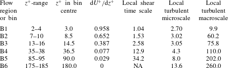
were qualitatively different from those at the channel centre. Now we aim to provide a complete coverage of the particle behaviour in different regions of the channel flow. We have therefore defined six different regions or bins in table 3 (shaded vertical bands in figure 1). The innermost bin B1 is centred around
 $z^{+}=3$
and is only two wall units
 $\unicode[STIX]{x1D708}/u_{\unicode[STIX]{x1D70F}}$
thick, whereas the central bin B6 is
 $10\unicode[STIX]{x1D708}/u_{\unicode[STIX]{x1D70F}}$
thick.
Variation of flow statistics across the turbulent channel flow at
 $Re_{\unicode[STIX]{x1D70F}}=180$
. (a) Streamwise mean velocity
 $\langle u^{+}\rangle$
(continuous line), the dotted lines represent linear and logarithmic variations; (b) root-mean-square of velocity fluctuations in the streamwise (solid line), wall-normal (dashed-dotted line) and cross-stream (dotted line) directions; (c) turbulent shear stress
 $-\langle \hat{u} ^{+}{\hat{w}}^{+}\rangle$
(solid line), viscous shear stress
 $\text{d}U^{+}/\text{d}z^{+}$
(dashed-dotted line) and total shear stress
 $-\langle \hat{u} ^{+}{\hat{w}}^{+}\rangle +\text{d}U^{+}/\text{d}z^{+}$
(dotted line); (d) root-mean-square of vorticity fluctuations in the three coordinate directions (same legend as in b). The symbols are DNS data at
 $Re_{\unicode[STIX]{x1D70F}}=178$
from Moser et al. (Reference Moser, Kim and Mansour1999) which closely reproduce the Kim, Moin & Moser (Reference Kim, Moin and Moser1987) simulation. Six bins B
 $i$
(
 $i=1,6$
) are indicated as shaded areas; see also table 3. The thicknesses of the bins increase towards the centre although the logarithmic
 $z^{+}$
-axis gives the false impression that B1 is the thickest bin.

The first bin B1 is located in the viscous sublayer where the mean velocity
 $U^{+}$
increases linearly with
 $z^{+}$
(see panel a) and the Reynolds shear stress
 $-\langle \hat{u} ^{+}{\hat{w}}^{+}\rangle$
in panel (c) is negligible in comparison with the viscous shear stress
 $\text{d}U^{+}/\text{d}z^{+}$
. Here, instantaneous velocity and vorticity components have been decomposed into mean and fluctuating parts, e.g.
 $u=\langle u\rangle +\hat{u}$
and
 $2\unicode[STIX]{x1D6FA}_{x}=\langle 2\unicode[STIX]{x1D6FA}_{x}\rangle +2\hat{\unicode[STIX]{x1D6FA}}_{x}$
, where angular brackets denote mean values and a circumflex (or ‘hat’) indicates the deviation from the mean, i.e. a fluctuation. Recall that the fluid vorticity is two times the rate of rotation
 $\unicode[STIX]{x1D734}$
in equation (2.4). The fluctuating velocity and vorticity fields are both approaching their respective two-component wall limits. Bins B2 and B3 are both in the buffer layer where
 $U^{+}<z^{+}$
and the velocity and vorticity fluctuations are distinctly anisotropic with
 $\langle \hat{u} ^{2}\rangle >\langle \hat{v}^{2}\rangle >\langle {\hat{w}}^{2}\rangle$
and
 $\langle (2\hat{\unicode[STIX]{x1D6FA}}_{y})^{2}\rangle >\langle (2\hat{\unicode[STIX]{x1D6FA}}_{z})^{2}\rangle >\langle (2\hat{\unicode[STIX]{x1D6FA}}_{x})^{2}\rangle$
. According to figure 1(c), however, the Reynolds shear stress
 $-\langle \hat{u} ^{+}{\hat{w}}^{+}\rangle$
is smaller than the viscous shear stress
 $\text{d}U^{+}/\text{d}z^{+}$
in B2, whereas
 $-\langle \hat{u} ^{+}{\hat{w}}^{+}\rangle$
exceeds
 $\text{d}U^{+}/\text{d}z^{+}$
in B3.
In bins B4 and B5 the mean velocity
 $U^{+}$
exhibits a logarithmic variation and the viscous shear stress is of negligible importance. The typical anisotropy of the velocity fluctuations persists, while the vorticity fluctuations almost exhibit isotropy; as discussed e.g. in Antonia, Kim & Browne (Reference Antonia, Kim and Browne1991) and Andersson et al. (Reference Andersson, Zhao and Variano2015). The velocity anisotropy remains all the way to the channel centre (B6) where the turbulent
 $-\langle \hat{u} ^{+}{\hat{w}}^{+}\rangle$
and viscous
 $\text{d}U^{+}/\text{d}z^{+}$
shear stresses both are zero for symmetry reasons.
The intricate way in which inertial particles interact with the viscous fluid depends not only on one or more particle time scales, e.g. those defined in equation (2.6), but also on relevant time scales of the fluid motion. The viscous or inner time scale
 $\unicode[STIX]{x1D70F}_{visc}=\unicode[STIX]{x1D708}/u_{\unicode[STIX]{x1D70F}}^{2}$
is representative of near-wall turbulence. The inverse of the mean shear rate, i.e.
 $\unicode[STIX]{x1D70F}_{shear}=(\text{d}U/\text{d}z)^{-1}$
, increases monotonically from the wall (where
 $\unicode[STIX]{x1D70F}_{shear}=\unicode[STIX]{x1D70F}_{visc}$
) to the channel centre. Notice that
 $\unicode[STIX]{x1D70F}_{shear}/\unicode[STIX]{x1D70F}_{visc}=(\text{d}U^{+}/\text{d}z^{+})^{-1}$
. Representative measures of the turbulence are the micro- and macroscales
 $\unicode[STIX]{x1D70F}_{\unicode[STIX]{x1D702}}$
and
 $\unicode[STIX]{x1D70F}_{\ell }$
, respectively, both of which are reported in table 3. The turbulent macroscale
 $\unicode[STIX]{x1D70F}_{\ell }$
is taken as the eddy turnover time
 $\langle \hat{u} _{i}\hat{u} _{i}\rangle /\unicode[STIX]{x1D700}$
(see Lee, Kim & Moin Reference Lee, Kim and Moin1990), where
 $\langle \hat{u} _{i}\hat{u} _{i}\rangle$
is twice the mean turbulent kinetic energy and
 $\unicode[STIX]{x1D700}$
is the energy dissipation rate. One can readily observe from the data compiled in table 3 that all the different time scales increase monotonically from the wall towards the channel centre. However, while the Kolmogorov microscale
 $\unicode[STIX]{x1D70F}_{\unicode[STIX]{x1D702}}$
is five times larger in the centre than in bin B1, other time scales vary even more. This is only one of the reasons for the qualitatively different behaviour of inertial particles in near-wall turbulence and in the almost isotropic channel centre, as discussed in Zhao et al. (Reference Zhao, Challabotla, Andersson and Variano2015).
Six representative flow regions Bi (
 $i=1$
, 6) with characteristic time scales calculated at the bin centres and scaled with
 $\unicode[STIX]{x1D70F}_{visc}$
.

The goal of the present work is to explore the modes of particle rotation all the way from the channel wall to the centre. Although we know that inertial spheroids behave qualitatively different in very-near-wall turbulence in the buffer region (bin B2) and at the centre (bin B6), not only the mean shear rate but also the fluctuating velocity and vorticity fields vary dramatically across the channel. A complete coverage of particle rotation behaviour will therefore be provided. In particular, we focus on the inner part of the logarithmic wall layer (bin B4), in which the fluid vorticity is nearly isotropic in spite of the dominance of the Reynolds shear stress over the viscous shear stress. This, in combination with the distinctly different time scales of the fluid motions, cf. table 3, makes it likely that spheroids in bin B4 rotate differently not only from those in the buffer region (wall mode) but also from those in the almost isotropic centre (centre mode).
3 Results
Simulations are performed for spheroids with five different aspect ratios
 $\unicode[STIX]{x1D706}=0.1$
, 0.33, 1, 3 and 10 and three different Stokes numbers
 $St=0$
, 1 and 30. The Stokes number
 $St$
is defined as the ratio between the particle response time
 $\unicode[STIX]{x1D70F}_{p}$
given in equation (2.6) and the viscous time scale
 $\unicode[STIX]{x1D70F}_{visc}=\unicode[STIX]{x1D708}/u_{\unicode[STIX]{x1D70F}}^{2}$
defined in § 2.3. This definition of the Stokes number serves primarily for bookkeeping in order to distinguish between spheroids with different inertia. Since the time scales of the fluid flow vary from the channel wall to the channel centre (see table 3), an effective Stokes number based on a local time scale of the flow field should be used to enable sound physical interpretations. Since these local scales (seen in table 3) are always greater than
 $\unicode[STIX]{x1D70F}_{visc}$
, the effective Stokes numbers represent maximum possible values. For a given aspect ratio
 $\unicode[STIX]{x1D706}$
, the Stokes number is altered by varying the density ratio
 $D$
. The simulations for
 $\unicode[STIX]{x1D706}=1$
are performed for
 $\unicode[STIX]{x1D706}=1.001$
to avoid the singularities of the tensor elements in table 1 and the shape factors in table 2.
For each of the fifteen particle parameter combinations, 500 000 spheroids with semi-axis
 $a^{+}=0.36$
are introduced randomly into the same fully developed turbulence field at
 $t=0$
. Orientational and rotational particle statistics are computed by averaging instantaneous data over the time window from
 $5400\unicode[STIX]{x1D70F}_{visc}$
to
 $10\,800\unicode[STIX]{x1D70F}_{visc}$
as well as in the homogeneous (streamwise and cross-stream) directions. We use the unit vector
 $\boldsymbol{p}$
aligned with the particle symmetry axis (
 $z^{\prime }$
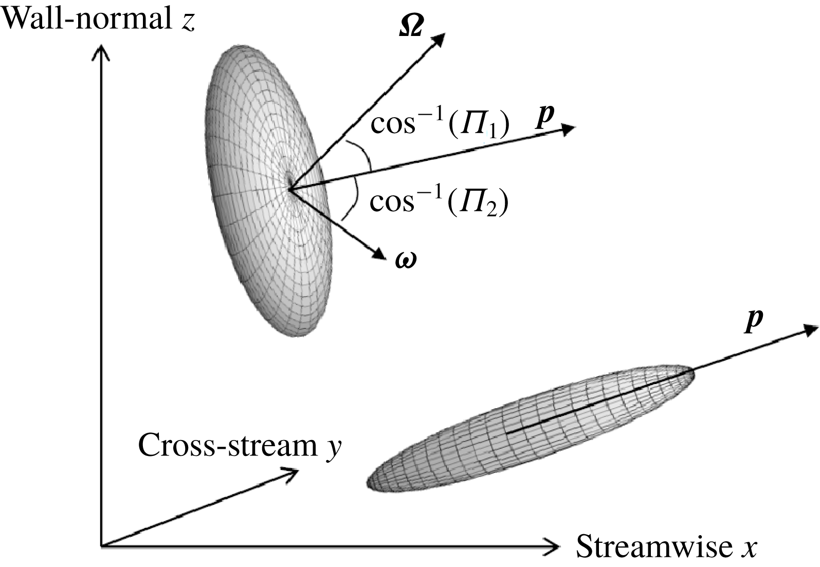
-axis) to identify particle orientations, see figure 2. The particle orientation parameters
 $\unicode[STIX]{x1D6F1}_{1}$
and
 $\unicode[STIX]{x1D6F1}_{2}$
measure the alignment of
 $\boldsymbol{p}$
with fluid rotation
 $\unicode[STIX]{x1D734}$
and particle rotation
 $\unicode[STIX]{x1D74E}$
, respectively.
Definition sketch of the particle orientation parameters
 $\unicode[STIX]{x1D6F1}_{1}$
and
 $\unicode[STIX]{x1D6F1}_{2}$
.
 $\unicode[STIX]{x1D6F1}_{1}=\boldsymbol{p}\boldsymbol{\cdot }\unicode[STIX]{x1D734}/|\boldsymbol{p}|\,|\unicode[STIX]{x1D734}|$
is a measure of the alignment of the orientation unit vector
 $\boldsymbol{p}$
with the fluid angular velocity
 $\unicode[STIX]{x1D734}$
. Similarly,
 $\unicode[STIX]{x1D6F1}_{2}=\boldsymbol{p}\boldsymbol{\cdot }\unicode[STIX]{x1D74E}/|\boldsymbol{p}|\,|\unicode[STIX]{x1D74E}|$
is a measure of the alignment of
 $\boldsymbol{p}$
with the particle angular velocity
 $\unicode[STIX]{x1D74E}$
. Laboratory coordinates
 $x$
,
 $y$
and
 $z$
are shown as well.

Ratio between mean particle angular velocity
 $\langle \unicode[STIX]{x1D714}_{i}\rangle \langle \unicode[STIX]{x1D714}_{i}\rangle$
and fluctuating particle angular velocities
 $\langle \hat{\unicode[STIX]{x1D714}}_{i}\hat{\unicode[STIX]{x1D714}}_{i}\rangle$
across the channel for
 $St=0$
(a);
 $St=1$
(b); and
 $St=30$
(c). Ratios below 0.5 indicate that fluctuating motions account for the majority of the mechanical energy associated with the particle rotation. Note that
 $\langle \unicode[STIX]{x1D714}_{j}\rangle \langle \unicode[STIX]{x1D714}_{j}\rangle =\langle \unicode[STIX]{x1D714}_{y}\rangle ^{2}$
due to the symmetry of the plane channel flow.

3.1 Eulerian particle orientation and rotation statistics
A particle’s angular velocity vector
 $\unicode[STIX]{x1D74E}$
can be decomposed into mean and fluctuating parts in order to distinguish between particle rotation caused by the mean shear rate
 $\text{d}U/\text{d}z$
and the turbulent flow field. The kinetic energy
 $\frac{1}{2}\langle \unicode[STIX]{x1D714}_{i}\rangle \langle \unicode[STIX]{x1D714}_{i}\rangle =\frac{1}{2}\langle \unicode[STIX]{x1D714}_{y}\rangle ^{2}$
associated with the mean particle rotation
 $\langle \unicode[STIX]{x1D714}_{i}\rangle$
stems entirely from rotation in the
 $x-z$
plane, whereas rotational fluctuations
 $\hat{\unicode[STIX]{x1D714}}_{i}$
in all three directions contribute to the kinetic energy
 $\frac{1}{2}\langle \hat{\unicode[STIX]{x1D714}}_{i}\hat{\unicode[STIX]{x1D714}}_{i}\rangle$
of the particle’s angular velocity fluctuations. Such results were presented by Challabotla et al. (Reference Challabotla, Zhao and Andersson2015c
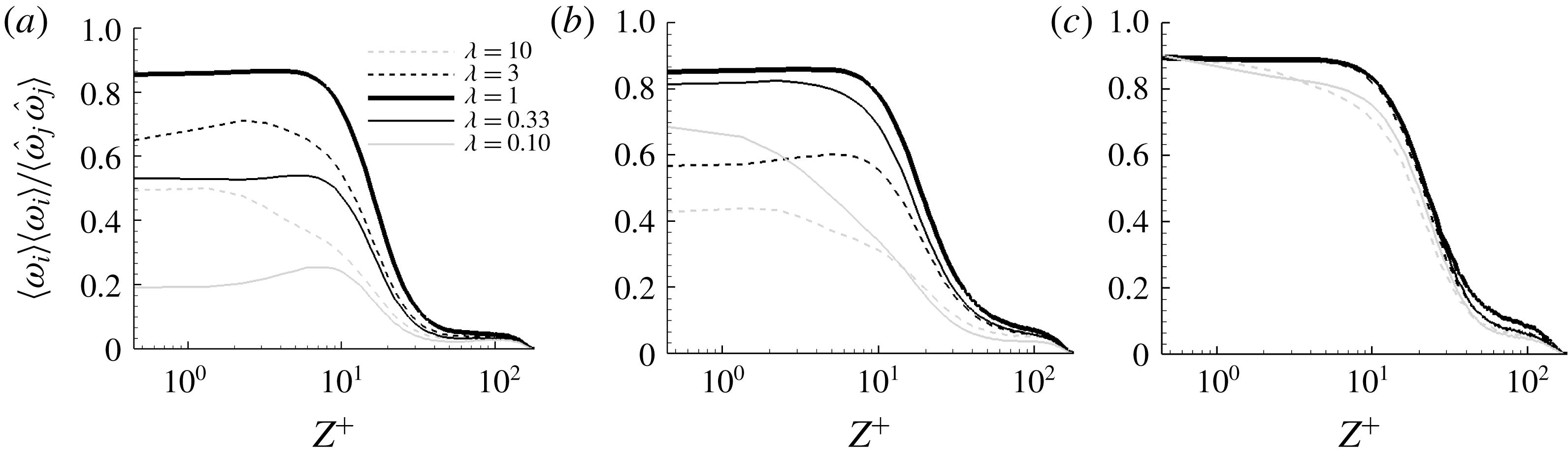
) and Marchioli & Soldati (Reference Marchioli and Soldati2013) for oblate and prolate inertial spheroids, respectively. Here, however, figure 3 shows the ratio between the kinetic energies associated with mean and fluctuating particle rotation. For the most inertial spheroids in figure 3(c), mean rotation dominates near the wall, whereas fluctuating rotation dominates in the central part of the channel. The transition between mean rotation and fluctuating rotation dominance, identified by the location at which
 $\langle \unicode[STIX]{x1D714}_{y}\rangle ^{2}$
drops below
 $\frac{1}{2}\langle \hat{\unicode[STIX]{x1D714}}_{i}\hat{\unicode[STIX]{x1D714}}_{i}\rangle$
, occurs over a fairly narrow region from
 $z^{+}\approx 10$
to 40. The effect of particle shape
 $\unicode[STIX]{x1D706}$
is modest and leads to a broadening of the transition zone for the most aspherical particles. The near-wall plateau up to
 $z^{+}\approx 10$
in figure 3(c) shows that the mean particle rotation in the cross-stream direction is dominant. This reflects the importance of mean shear in the near-wall region.
The near-wall dominance of mean shear on inertia-free particles in figure 3(a) is, however, present only for near-spherical particles. The longest rods and the flattest disks are mostly affected by fluctuating rotation even in the near-wall region. The transition zone between mean rotation and fluctuating rotation dominance is gradually shifted away from the wall with increasing particle inertia. We, therefore, infer that particle angular velocity fluctuations dominate over the mean angular velocity over a fairly wide central part of the channel. Particle inertia somewhat reduces this effect since inertial particles are able to partially withstand turbulent fluctuations whose time scale is short.
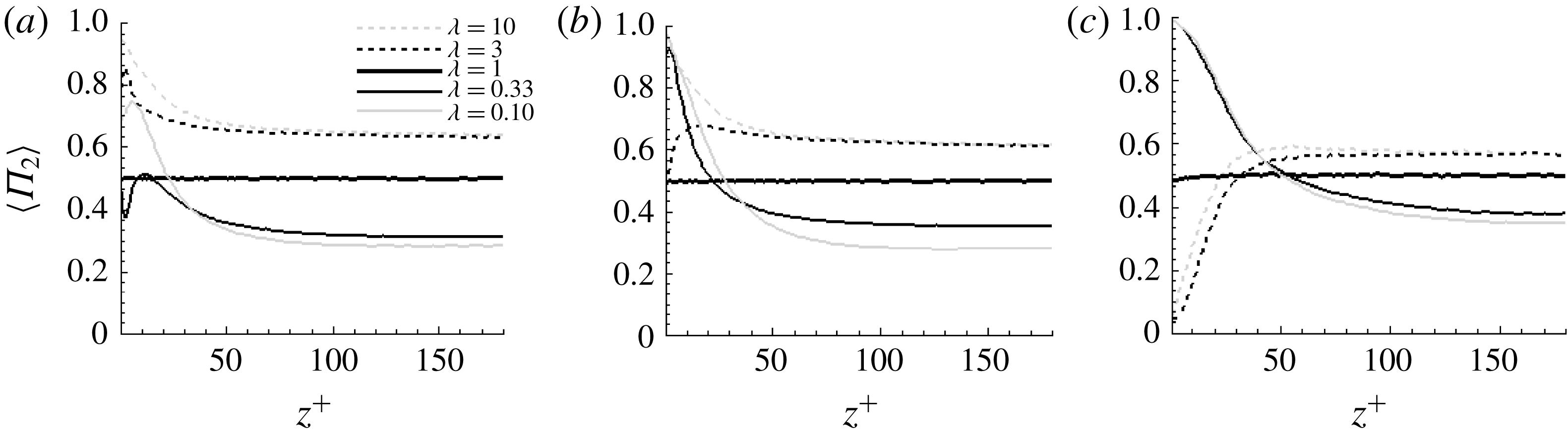
Figure 4 shows the mean alignment between a particle’s direction
 $\boldsymbol{p}$
and its angular velocity vector
 $\unicode[STIX]{x1D74E}$
, as quantified by the orientation parameter
 $\langle \unicode[STIX]{x1D6F1}_{2}\rangle$
defined in figure 2. Perfect alignment between a particle and its angular velocity vector, i.e.
 $\langle \unicode[STIX]{x1D6F1}_{2}\rangle =1.0$
, suggests spinning motion, whereas particle alignment orthogonal to
 $\unicode[STIX]{x1D74E}$
, i.e.
 $\langle \unicode[STIX]{x1D6F1}_{2}\rangle =0$
, suggests tumbling motion. In the near-wall region, say
 $z^{+}<30$
, inertialess rod-like particles (
 $St=0$
) preferentially align with their angular velocity vectors (
 $\langle \unicode[STIX]{x1D6F1}_{2}\rangle >0.5$
), but this tendency becomes weaker with increasing inertia until the most inertial rods (
 $St=30$
) align almost perpendicularly to their angular velocity vector (
 $\langle \unicode[STIX]{x1D6F1}_{2}\rangle \approx 0$
). We can, therefore, infer that prolate spheroids in the wall vicinity exhibit a transition from dominant spinning motion to tumbling motion as particle inertia increases. In contrast, the flattest oblate spheroids align with their rotation vector in the near-wall region. This alignment increases with inertia and suggests that oblate spheroids are spinning rather than tumbling in the mean-shear-dominated wall region.
Across the central half of the channel, the orientation parameter
 $\langle \unicode[STIX]{x1D6F1}_{2}\rangle$
is almost constant and above and below 0.5 for prolate and oblate spheroids, respectively. This suggests preferential spinning of rods and tumbling of disks. This finding is consistent with observations by Parsa et al. (Reference Parsa, Calzavarini, Toschi and Voth2012) and Byron et al. (Reference Byron, Einarsson, Gustavsson, Voth, Mehlig and Variano2015) in HIT and supports their explanation that particle rotation results from the alignment of vorticity and extensional strain in HIT. The vorticity field in the channel centre is almost isotropic (Andersson et al.
Reference Andersson, Zhao and Variano2015) and this isotropy persists from the centre and all the way to
 $z^{+}\approx 36$
, i.e. bin B4 in figure 1(d). This is likely to explain why the orientation parameter
 $\langle \unicode[STIX]{x1D6F1}_{2}\rangle$
remains approximately constant over a major portion of the turbulent channel, especially for the inertialess particles in figure 4(a).
Investigations of rotation of inertial particles in simple shear flow by Lundell & Carlsson (Reference Lundell and Carlsson2010) and Einarsson et al. (Reference Einarsson, Angilella and Mehlig2014) showed that the stable attractor for inertial rods is tumbling in the velocity-gradient plane. Prolate spheroids (
 $\unicode[STIX]{x1D706}=3$
, 10) with
 $St=30$
show this behaviour, as well as a linear transition from nearly pure tumbling close to the wall (bin B1) to a value
 $\langle \unicode[STIX]{x1D6F1}_{2}\rangle \approx 0.55$
in bin B4 that remains constant all through bins B5 and B6. This transition closely mirrors the behaviour of the mean viscous shear stress, i.e. large in B1 and constant from B4–B6. Oblate spheroids (
 $\unicode[STIX]{x1D706}=0.33$
, 0.1) with
 $St=30$
show a similar transition in alignment statistics, moving from nearly pure spinning near the wall (bin B1) to a value
 $\langle \unicode[STIX]{x1D6F1}_{2}\rangle \approx 0.4$
that remains nearly constant from bin B4 to B6. Lower inertia leads to smaller changes and a larger variety in behaviour.
To understand why spheroidal particles behave this way, an in-depth analysis of the co-variances between particle orientation
 $\boldsymbol{p}$
, particle rotation
 $\unicode[STIX]{x1D74E}$
and fluid rotation
 $\unicode[STIX]{x1D734}$
is required. In order to uncover the subtle dynamics of non-spherical particles, we take a closer look into the particle behaviour in B2 (near wall), B4 (transition) and B6 (channel centre). The qualitatively different flow characteristics in these bins have already been described in § 2.3.
Alignment between a particle’s symmetry axis
 $\boldsymbol{p}$
and its angular velocity vector
 $\unicode[STIX]{x1D74E}$
across the channel for
 $St=0$
(a),
 $St=1$
(b) and
 $St=30$
(c). The normalized measure
 $\unicode[STIX]{x1D6F1}_{2}$
is defined in the caption to figure 2. Values on the vertical axis less than 0.5 indicate that tumbling motions are responsible for most of a particle’s angular velocity.

3.2 Co-variances of particle orientation, particle rotation and fluid vorticity
Co-variances between particle orientation
 $\boldsymbol{p}$
, particle rotation
 $\unicode[STIX]{x1D74E}$
and local fluid rotation
 $\unicode[STIX]{x1D734}$
are explored in this sub-section. We first analyse the instantaneous alignment of a spheroidal particle with respect to particle and fluid angular velocity vectors in figures 5–7. We thereafter examine co-variances of
 $\boldsymbol{p}$
,
 $\unicode[STIX]{x1D74E}$
and
 $\unicode[STIX]{x1D734}$
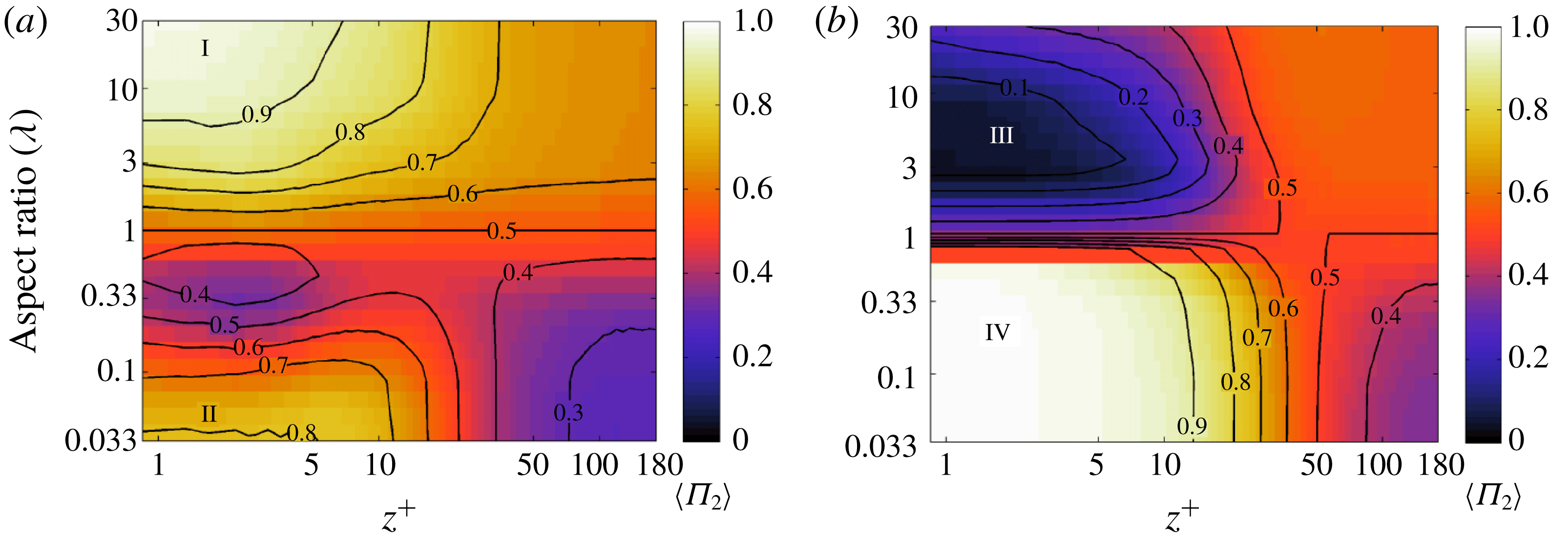
by means of ternary scatter plots in figures 8–11. Such in-depth examinations are provided for particles in three of the six bins defined in § 2.3. Finally, a continuous mapping of the particles’ rotation modes all the way from the wall to the channel centre is provided in figure 12 in § 3.3.
The particle’s alignment with its rotation vector is measured by means of the particle orientation parameter
 $\unicode[STIX]{x1D6F1}_{2}$
and shown already in figure 4. Now the covariances between the particle’s alignment with its rotation (measured by
 $\unicode[STIX]{x1D6F1}_{2}$
) and particle alignment with the fluid rotation (measured by
 $\unicode[STIX]{x1D6F1}_{1}$
) are considered. Recall that when a particle is aligned with its angular velocity vector (
 $\unicode[STIX]{x1D6F1}_{2}=1$
on the vertical axis in figure 5), this indicates spinning motion; when a particle is aligned orthogonally to its angular velocity vector (
 $\unicode[STIX]{x1D6F1}_{2}=0$
on the vertical axis), this indicates tumbling motion. The
 $\unicode[STIX]{x1D6F1}_{2}=\unicode[STIX]{x1D6F1}_{1}$
line may indicate that particle’s angular velocity is aligned with the fluid vorticity. In particular, whenever
 $\unicode[STIX]{x1D6F1}_{2}=\unicode[STIX]{x1D6F1}_{1}=1$
, i.e. in the upper right corner of the scatter plots,
 $\unicode[STIX]{x1D74E}$
is parallel with
 $\unicode[STIX]{x1D734}$
. Histograms on each axis show the likelihood of finding a particle in a given alignment. Weighting the histograms by the angular velocity magnitude (i.e. moving from green curves to red curves) causes no significant change in histogram shape. The first moment of the vertical axis histogram is extracted and used later in the summary of particle behaviour in figure 12.
Scatter plots of
 $\unicode[STIX]{x1D6F1}_{1}$
versus
 $\unicode[STIX]{x1D6F1}_{2}$
, i.e. alignment of particle orientation
 $\boldsymbol{p}$
relative to the fluid vorticity
 $2\unicode[STIX]{x1D734}$
and relative to particle angular velocity
 $\unicode[STIX]{x1D74E}$
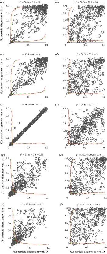
. All plots show data from the channel centre (bin B6). The size of each point in the scatter plot represents the magnitude of particle angular velocity for that sample. In each panel the two green curves show the probability distribution of alignment (i.e. the sum of scatter data over one dimension) and the two red curves show the same distribution, but weighted by the magnitudes of each sample (i.e. accounting for the size of each dot in the scatter data). From top to bottom the particle shape varies from
 $\unicode[STIX]{x1D706}=10$
(a,b), 3 (c,d), 1 (e,f), 0.33 (g,h) and 0.1 (i,j). Left column represents cases with
 $St=0$
and right column is for
 $St=30$
.

Clustering of samples indicates preferential alignment of spheroids relative to the vectors of fluid rotation and particle rotation. First of all, we observe that the samples in the channel centre (bin B6) for inertialess rods are clustered at the right top corner in figure 5(a,c) where both
 $\unicode[STIX]{x1D6F1}_{1}$
and
 $\unicode[STIX]{x1D6F1}_{2}\approx 1$
. This is an important (and straightforward) location in parameter space. It tells us that rods align with fluid vorticity and spin. Inertialess disks (figure 5
g,i) occupy the other important and straightforward location in parameter space, namely
 $\unicode[STIX]{x1D6F1}_{1}\approx \unicode[STIX]{x1D6F1}_{2}\approx 0$
. This shows that disks align normal to fluid vorticity and tumble. This information was already seen in figure 4, but the scatter plot shows additional information. The distribution of points in parameter space is unimodal, i.e. there is one basin of attraction and noise that spreads the particles away from this. Such a case is substantially different than a hypothetical case in which there are multiple points of clustering that would indicate multiple preferred modes of rotation.
Observed shape effects on the preferential alignments and rotations of tracer spheroids (
 $St=0$
) at the channel centre are consistent with the earlier findings in homogenous isotropic turbulence (Parsa et al.
Reference Parsa, Calzavarini, Toschi and Voth2012; Marcus et al.
Reference Marcus, Parsa, Kramel, Ni and Voth2014; Byron et al.
Reference Byron, Einarsson, Gustavsson, Voth, Mehlig and Variano2015). The rotation mode of inertialess spheroids is determined by the alignment of the particles relative to fluid rotation. Zhao & Andersson (Reference Zhao and Andersson2016) showed that at the channel centre inertialess rods (alternatively disks) align parallel to (alternatively normal to) the direction of Lagrangian fluid stretching. Fluid rotation also tends to orient in the Lagrangian stretching direction. Therefore, a rod-like particle rotates in the direction of fluid rotation (spinning), but a disk-like particle rotates normal to the fluid rotation (tumbling). The mechanism that causes this rotation mode is the same in the channel centre as in HIT. Additionally, as one could expect, spheres due to their isotropic shape align randomly relative to both fluid and particle rotations, as seen from the histograms in figure 5(e).
By comparing the panels in the right column of figure 5 for inertial spheroids (
 $St=30$
) with those in the left column for inertialess particles, we observe weakened preferential clustering (more scatter) for the inertial particles. This reveals that particle inertia damps the preferential alignment relative to both fluid and particle rotations. Unsurprisingly, the preferential spinning and tumbling motions are attenuated, but no new preferences arise relative to the tracer spheroids. This finding of the inertial effect on particle preferential rotation is consistent with the study by Zhao et al. (Reference Zhao, Challabotla, Andersson and Variano2015) and measurements in HIT by Sabban et al. (Reference Sabban, Cohen and van Hout2017). Particle inertia filters the influence of short time scale turbulence fluctuations. Inertial particles thus respond only to fluid motions with relatively larger time scales. This attenuates not only the preferential alignment relative to the fluid rotation, but also any preferred rotation mode, i.e. spinning or tumbling. Chen, Jin & Zhang (Reference Chen, Jin and Zhang2016) performed a large-eddy simulation (LES) study of dynamics of tracer ellipsoids in isotropic turbulence and observed that a lack of subgrid-scale (SGS) turbulence weakens the preferential alignment between particle and vorticity. This, in turn, resulted in a more isotropic rotational behaviour regardless of particle shape. Here, we find that increasing particle inertia has a similar effect on particle alignment as discarding SGS fluctuations in LES. This finding can help design SGS closures aimed at LES of turbulent flows laden with inertial particles. The local scales of the fluid motion are moreover essential in micro-particle dynamics. Since the Kolmogorov time scale
 $\unicode[STIX]{x1D70F}_{\unicode[STIX]{x1D702}}$
in the channel centre increases with the Reynolds number, the effective Stokes number
 $\unicode[STIX]{x1D70F}_{p}/\unicode[STIX]{x1D70F}_{\unicode[STIX]{x1D702}}$
decreases with increasing
 $Re$
. This reduction of the effective Stokes number with increasing
 $Re$
makes us conclude that the influence of inertia weakens at higher
 $Re$
.
The rotational behaviour of spheroidal particles in the centre of the channel flow, as seen in figure 5, closely resembles particle rotation in HIT. Two conditions for this close similarity are met: (i) the vorticity fluctuations are almost isotropic, as shown by Andersson et al. (Reference Andersson, Zhao and Variano2015), and (ii) the mean shear rate
 $\text{d}U/\text{d}z$
(and thus the mean vorticity) is zero since the mean velocity
 $U(z)$
is symmetric about the channel centre. The innermost part of the logarithmic region, e.g. bin B4, is characterized by presence of mean shear and highly anisotropic velocity fluctuations. The vorticity fluctuations, however, still remain almost isotropic, contrary to in the buffer region which is to be explored later. We observe from the left column in figure 6 that tracer spheroids in bin B4 behave similarly to those at the centre of the channel. In general, rod-like tracers tend to align in the direction of local fluid rotation, which leads to spinning motion, while disk-like particles orient preferentially normal to the fluid rotation resulting in tumbling motion. Although the rotation modes of tracers remain the same in bin B4 as in bin B6, the magnitude of the rotation
 $|\unicode[STIX]{x1D74E}|$
is augmented due to the presence of mean shear in the logarithmic layer.
Scatter plots of
 $\unicode[STIX]{x1D6F1}_{1}$
versus
 $\unicode[STIX]{x1D6F1}_{2}$
, i.e. alignment
 $\boldsymbol{p}$
of particle relative to the fluid vorticity
 $2\unicode[STIX]{x1D734}$
and relative to particle angular velocity
 $\unicode[STIX]{x1D74E}$
. All plots show data from bin B4. The size of each point in the scatter plot represents the magnitude of particle angular velocity for that sample. In each panel the two green curves show the probability distribution of alignment (i.e. the sum of scatter data over one dimension) and the two red curves show the same distribution, but weighted by the magnitudes of each sample (i.e. accounting for the size of each dot in the scatter data). From top to bottom the particle shape varies from
 $\unicode[STIX]{x1D706}=10$
(a,b), 3 (c,d), 1 (e,f), 0.33 (g,h) and 0.1 (i,j). Left column represents the cases with
 $St=0$
and right column is for
 $St=30$
.

Scatter plots of
 $\unicode[STIX]{x1D6F1}_{1}$
versus
 $\unicode[STIX]{x1D6F1}_{2}$
, i.e. alignment
 $\boldsymbol{p}$
of the particle relative to the fluid vorticity
 $2\unicode[STIX]{x1D734}$
and relative to particle angular velocity
 $\unicode[STIX]{x1D74E}$
in the buffer layer (bin B2). The size of each point in the scatter plot represents the magnitude of the particle angular velocity for that sample. In each panel the two green curves show the probability distribution of alignment (i.e. the sum of scatter data over one dimension) and the two red curves show the same distribution, but weighted by the magnitudes of each sample (i.e. accounting for the size of each dot in the scatter data). From top to bottom the particle shape varies from
 $\unicode[STIX]{x1D706}=10$
(a,b), 3 (c,d), 1 (e,f), 0.33 (g,h) and 0.1 (i,j). Left column represents the cases with
 $St=0$
and right column is for
 $St=30$
.

Inertia causes spheroids to rotate qualitatively different in the logarithmic region. The scatters are more evenly distributed in the plots to the right in figure 6, thereby reflecting a weakened alignment of
 $\boldsymbol{p}$
with both fluid and particle rotation vectors. This, in turn, reduces the dependence of particle alignment on particle shape. The two different rotation modes observed in the channel centre and in the buffer region by Zhao et al. (Reference Zhao, Challabotla, Andersson and Variano2015) are outcomes of two fundamentally different mechanisms, one which has already been discussed in conjunction with figure 5, and the other one which will be addressed when scatters from bin B2 are to be considered in figure 7. The almost negligible alignments found in the log layer is therefore likely to be the outcome of a delicate balance between these two mechanisms, in combination with the scrambling caused by vigorous velocity and vorticity fluctuations.
The reduced alignments of inertial spheroids explain why the preferences towards either spinning (of rods) or tumbling (of disks) observed in the channel centre are almost absent in the log layer. Inspection of the histograms in figure 6(h,j) shows that disk-like particles orient randomly with respect to the fluid rotation
 $\unicode[STIX]{x1D734}$
, but modestly align with their rotation vector
 $\unicode[STIX]{x1D74E}$
. This tendency of disks towards spinning rather than tumbling is contradictory to the behaviour in the channel centre, see figure 5(h,j).
The alignment of particles relative to the fluid vorticity
 $2\unicode[STIX]{x1D734}$
(horizontal axis) and particle rotational vector
 $\unicode[STIX]{x1D74E}$
(vertical axis) in the buffer layer at
 $z^{+}\approx 8$
is examined in the scatter plots shown in figure 7. The size of each scatter, which represents the magnitude of particle angular velocity
 $\unicode[STIX]{x1D74E}$
, is substantially larger than those in figures 5 and 6. The high particle rotation rate is caused by a more than 8-fold increase in mean shear rate
 $\text{d}U/\text{d}z$
in bin B2 than in bin B4; see the relevant entries in table 3.
Inertialess rods exhibit a stronger preferential alignment with the particle angular velocity
 $\unicode[STIX]{x1D74E}$
(since the scatters are clustered along the top of figure 7(a,c) where
 $\unicode[STIX]{x1D6F1}_{2}\approx 1$
), thereby indicating stronger spinning dominance than in the channel centre. The preferential particle alignment with the direction of the fluid rotation is, however, reduced from bin B6 to bin B2. Similarly to tracer rods, flat inertialess disks tend to align parallel to their rotation (
 $\unicode[STIX]{x1D6F1}_{2}\approx 1$
) and thus preferentially spin, but preferentially align normal to the direction of the fluid angular velocity (
 $\unicode[STIX]{x1D6F1}_{1}\approx 0$
). The smaller-sized scatters in the upper-left part of the plot suggest that disks rotate more slowly when
 $\unicode[STIX]{x1D6F1}_{1}$
is small, i.e. when disks primarily rotate with their symmetry axis perpendicular to the fluid vorticity.
Samples from spherical-shaped particles lie everywhere along the
 $\unicode[STIX]{x1D6F1}_{2}=\unicode[STIX]{x1D6F1}_{1}$
line in figure 7(e) and the distinction between spinning and tumbling rotation becomes irrelevant. The size of the scatters are substantially larger than in bins B4 and B6, simply because spheres rotate faster in the vicinity of the wall due to the monotonically increasing mean shear rate as the wall is approached. Tight clustering on the
 $\unicode[STIX]{x1D6F1}_{2}=\unicode[STIX]{x1D6F1}_{1}$
line indicates that particle angular velocity is very well aligned with fluid vorticity and no ‘angular slip velocity’
 $\unicode[STIX]{x1D74E}-\unicode[STIX]{x1D734}$
exists for inertialess spheres. This is indeed consistent with equating the Jeffery torque
 $\boldsymbol{N}$
in equation (2.4) to zero. An angular slip velocity does exist, however, for inertial spheres and spheroids, as discussed by Mortensen et al. (Reference Mortensen, Andersson, Gillissen and Boersma2007) and Marchioli, Zhao & Andersson (Reference Marchioli, Zhao and Andersson2016), respectively.
Two notable departures from the
 $\unicode[STIX]{x1D6F1}_{2}=\unicode[STIX]{x1D6F1}_{1}$
line can be seen in figure 7. First, asphericity pulls particles off the diagonal, showing that hybrids of spinning and tumbling are dynamically unfavourable. Second, inertia introduces angular slip – particles (even spheres) do not immediately reach equilibrium with the local flow. The first departure from the
 $\unicode[STIX]{x1D6F1}_{2}=\unicode[STIX]{x1D6F1}_{1}$
line is asymmetric, such that both rods and disks tend towards spinning behaviour. The samples that appear in the upper-left corner indicate motions that we did not expect to see. Specifically, spheroids spin about their symmetry axes orthogonal to the fluid vorticity, which makes disks move like a frisbee thrown along the channel’s streamwise axis and makes rods move like a drill while translating and spinning in the streamwise direction. This behaviour is unexpected because it seems to ignore the presence of fluid mean vorticity in the cross-stream direction. We explain it as follows: the spinning modes (drill or frisbee for rod and disk, respectively) appear if the particle is (i) spinning as it tumbles and (ii) pauses in the tumble cycle when the long axis is aligned in the streamwise direction. Condition (i) is met because the outer core-region flow perturbs particles away from any preferential spinning or tumbling, and condition (ii) is met because of streamwise alignment of the long axis due to preferential orientation of Lagrangian fluid stretching and compression in near-wall turbulence (Zhao & Andersson Reference Zhao and Andersson2016). This latter phenomenon is also known from Jeffery orbits in simple shear flows, which certainly hinders tumbling rotation with alignment in the streamwise direction. The half of parameter space which is nearly empty represents a tumbling mode with symmetry axis directed along the fluid vorticity axis. Such a state would not last long, as the tumbling would take the symmetry axis out of alignment, except at two instants of the tumbling cycle – most samples from such a cycle would appear at
 $\unicode[STIX]{x1D6F1}_{2}\approx \unicode[STIX]{x1D6F1}_{1}\approx 0$
.
The stronger clustering of scatters in the right column of figure 7 shows that particle inertia strengthens preferential alignment. This is opposite to the effect of inertia at the channel centre, where inertia leads to weaker clustering of scatters (i.e. a broader distribution). The opposite effect of inertia is due to the presence of mean shear in the log layer. Inertial rod-like particles align normal to both fluid and particle angular velocity vectors (scatters are around the lower-left corner in figure 7
b,d), implying strong tumbling motion compared with tracer rods in figure 7(a). Inertial disks align parallel both with
 $\unicode[STIX]{x1D734}$
and
 $\unicode[STIX]{x1D74E}$
(scatters are around top-right corner in figure 7
h,j), showing dominant spinning motion, in accordance with earlier observations by Challabotla et al. (Reference Challabotla, Zhao and Andersson2015c
). Both inertial rods and disks tend to rotate and align their major axes in the velocity-gradient plane (
 $x$
–
 $z$
plane), i.e. perpendicular to the direction of mean fluid rotation
 $\unicode[STIX]{x1D6FA}_{y}$
. This preferential alignment is probably caused by joint effects of particle inertia and mean shear and is seen to promote tumbling of rods and spinning of disks. As we already discussed, the influence of small-scale fluid motions is filtered by particle inertia so that mean shear becomes dominant. We accordingly assume that the particle dynamics in the vicinity of a wall is similar to the behaviour in a simple shear flow, in which inertia was found to drive a particle to align in the velocity-gradient plane (Lundell & Carlsson Reference Lundell and Carlsson2010; Challabotla et al.
Reference Challabotla, Nilsen and Andersson2015a
).
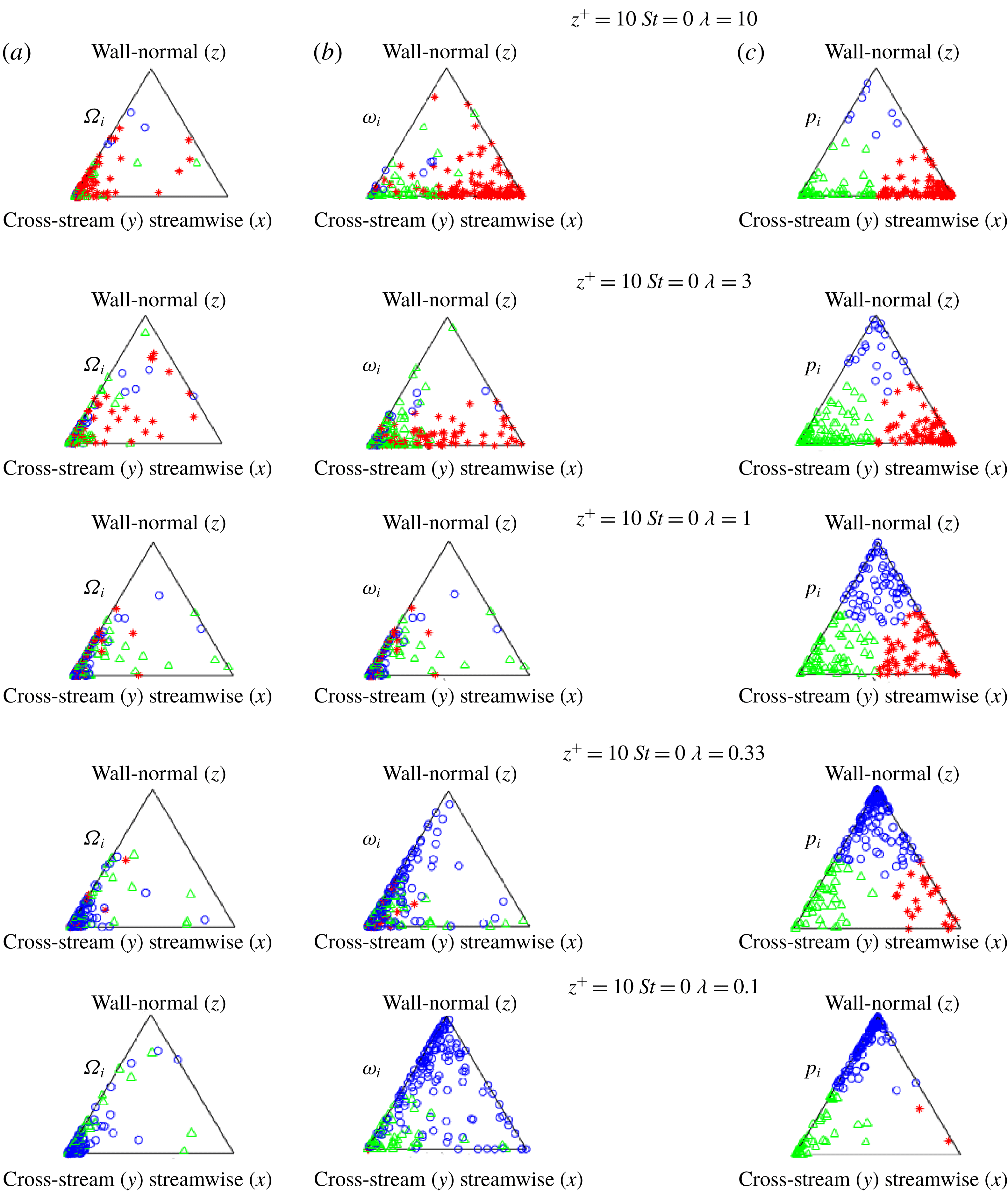
Near-wall orientation triangles for inertialess (
 $St=0$
) spheroids in the buffer layer (bin B2). Fluid rotation vector
 $\unicode[STIX]{x1D734}$
at a particle location (a), the particle angular velocity vector
 $\unicode[STIX]{x1D74E}$
(b) and particle orientation vector
 $\boldsymbol{p}$
(c). The aspect ratio
 $\unicode[STIX]{x1D706}$
decreases from 10 to 0.1 (rods on top, disks at the bottom). Each triangle shows 150 randomly selected instantaneous samples colour coded by the dominant direction of the particle orientation vector
 $\boldsymbol{p}$
. Red stars, green triangles and blue circles represent spheroids with preferential orientation in the streamwise, cross-stream (i.e. spanwise) and wall-normal directions, respectively.

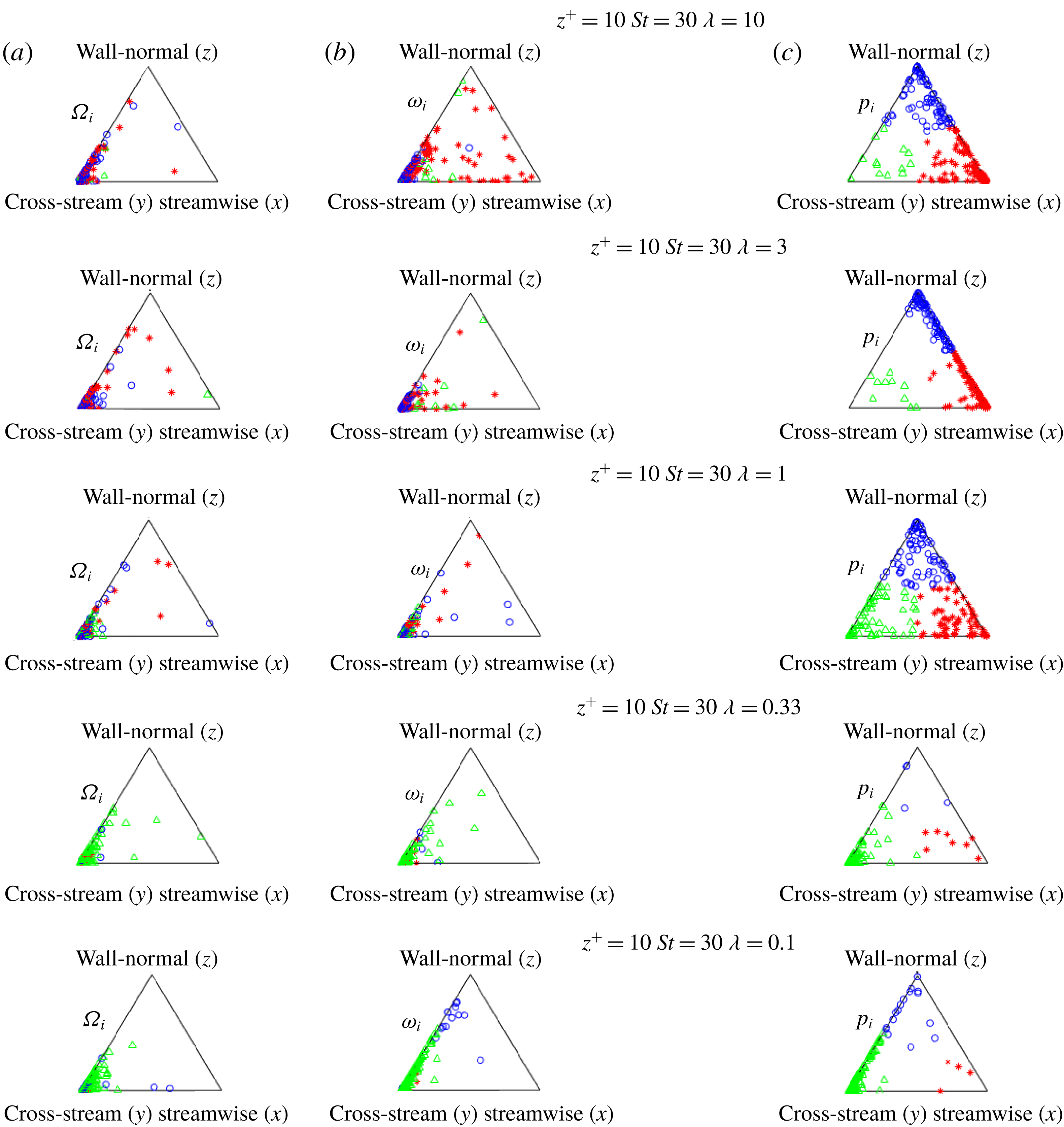
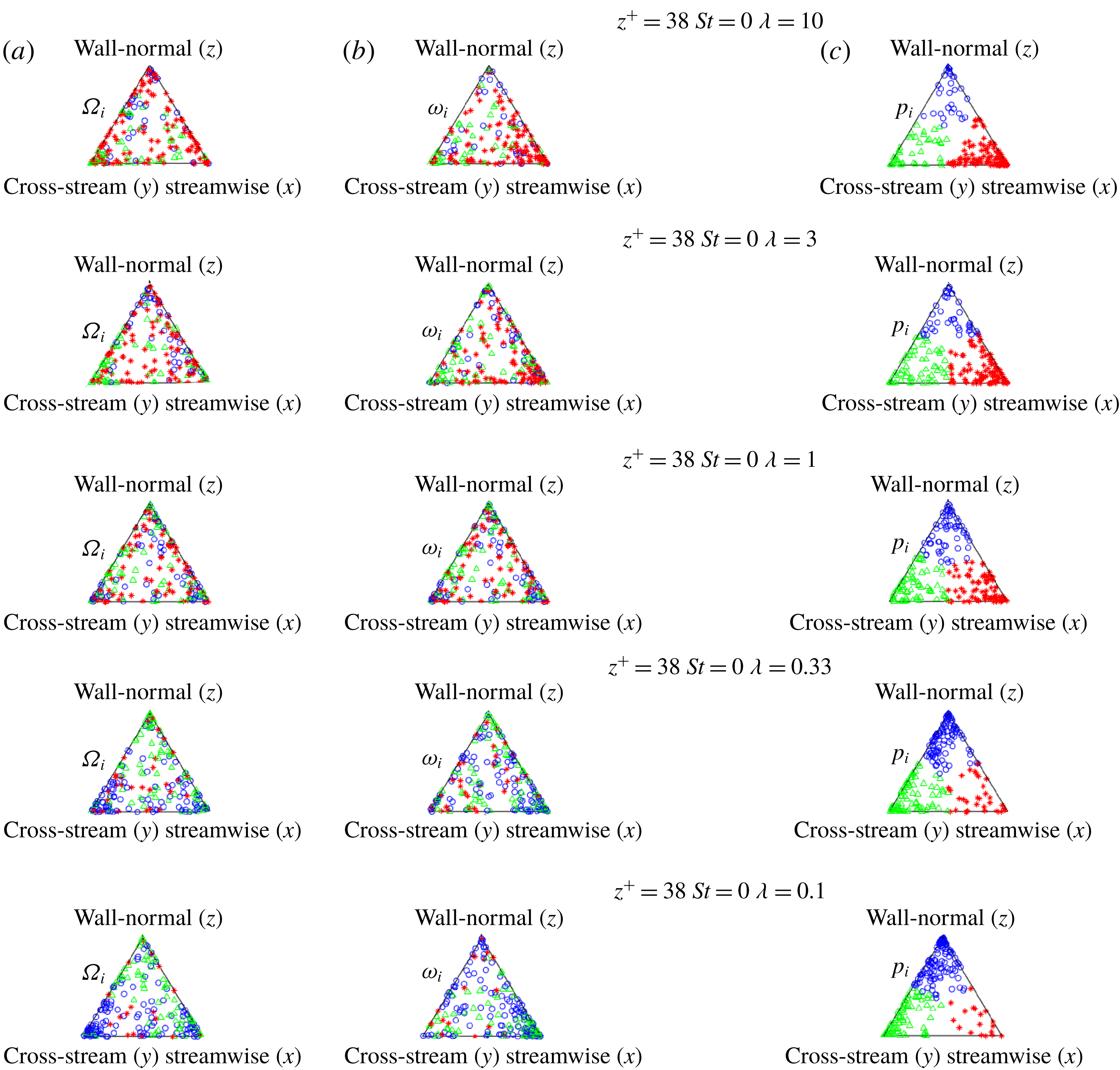
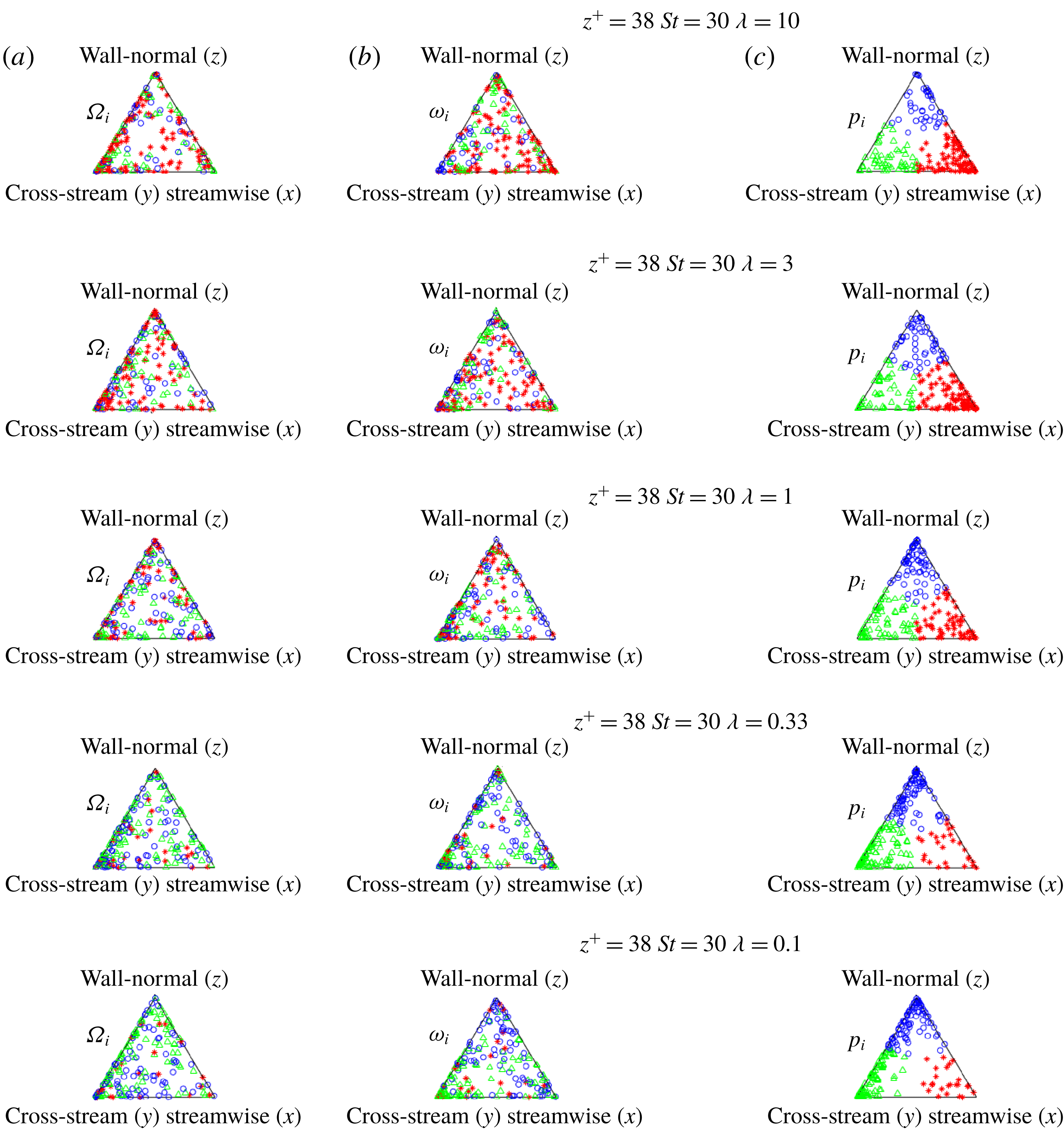
To further explore the observed complexity of particle orientation and rotation in detail, we examine the ternary scatter plots of fluid rotation (
 $\unicode[STIX]{x1D734}$
: left), particle rotation (
 $\unicode[STIX]{x1D74E}$
: centre) and particle orientation (
 $\boldsymbol{p}$
: right), in figures 8–11. This presentation helps to identify how spheroids are orientated relative to the laboratory coordinate axes (
 $x$
: streamwise,
 $y$
: cross-stream and
 $z$
: wall normal), information which is not uncovered when conventional particle alignment statistics, i.e.
 $\boldsymbol{p}\boldsymbol{\cdot }\unicode[STIX]{x1D74E}$
are shown, e.g. in figure 4. This presentation also helps in distinguishing different modes of spinning and tumbling relative to the three laboratory coordinate axes. The dominant mode of rotation is identified by comparing the last two columns: the same coloured scatters clustered at the same corner of the two columns indicate spinning mode, and different coloured scatters clustered at the same corner indicate tumbling mode. Examining corners with scatters tells us which type of tumbling or spinning is occurring. For instance, in the top triangles of figure 8 that describe tracer rods with
 $\unicode[STIX]{x1D706}=10$
, there are two co-existing spinning modes: one in the cross-stream direction (standard ‘log-rolling’ spinning) and one in the streamwise direction (a ‘drill-type’ spinning).
Near-wall orientation triangles for inertial (
 $St=30$
) spheroids in the buffer layer (bin B2). Fluid rotation vector
 $\unicode[STIX]{x1D734}$
at a particle location (a), particle angular velocity vector
 $\unicode[STIX]{x1D74E}$
(b) and particle orientation vector
 $\boldsymbol{p}$
(c). The aspect ratio
 $\unicode[STIX]{x1D706}$
decreases from 10 to 0.1 (rods on top, disks at the bottom). Each triangle shows 150 randomly selected instantaneous samples colour coded by the dominant direction of the particle orientation vector
 $\boldsymbol{p}$
. Red stars, green triangles and blue circles represent spheroids with preferential orientation in the streamwise, cross-stream (i.e. spanwise) and wall-normal directions, respectively.

Orientation triangles for inertialess (
 $St=0$
) spheroids in the logarithmic layer (bin B4). Fluid rotation vector
 $\unicode[STIX]{x1D734}$
at a particle location (a), particle angular velocity vector
 $\unicode[STIX]{x1D74E}$
(b) and particle orientation vector
 $\boldsymbol{p}$
(c). The aspect ratio
 $\unicode[STIX]{x1D706}$
decreases from 10 to 0.1 (rods on top, disks at the bottom). Each triangle shows 150 randomly selected instantaneous samples colour coded by the dominant direction of the particle orientation vector
 $\boldsymbol{p}$
. Red stars, green triangles and blue circles represent spheroids with preferential orientation in the streamwise, cross-stream (i.e. spanwise) and wall-normal directions, respectively.

Orientation triangles for inertialess (
 $St=30$
) spheroids in the B4. Fluid rotation vector
 $\unicode[STIX]{x1D734}$
at a particle location (a), the particle angular velocity vector
 $\unicode[STIX]{x1D74E}$
(b) and particle orientation vector
 $\boldsymbol{p}$
(c). The aspect ratio
 $\unicode[STIX]{x1D706}$
decreases from 10 to 0.1 (rods on top, disks at the bottom). Each triangle shows 150 randomly selected instantaneous samples colour coded by the dominant direction of the particle orientation vector
 $\boldsymbol{p}$
. Red stars, green triangles and blue circles represent spheroids with preferential orientation in the streamwise, cross-stream (i.e. spanwise) and wall-normal directions, respectively.

Contour plots of the orientation parameter
 $\langle \unicode[STIX]{x1D6F1}_{2}\rangle$
of (a) inertialess spheroids
 $St=0$
and (b) inertial spheroids
 $St=30$
.
 $\unicode[STIX]{x1D6F1}_{2}$
defined in figure 2 represents particle orientation
 $\boldsymbol{p}$
relative to particle rotation
 $\unicode[STIX]{x1D74E}$
. Therefore,
 $\unicode[STIX]{x1D6F1}_{2}\approx 1$
indicates spinning mode and
 $\unicode[STIX]{x1D6F1}_{2}\approx 0$
indicates tumbling mode. These plots were based on simulation results for ten different values of particle aspect ratio
 $\unicode[STIX]{x1D706}$
in the range from 0.01 to 50.

The preferential fluid rotation in the cross-stream direction caused by the dominant wall shear is captured via the clustering of
 $\unicode[STIX]{x1D734}$
at the left corner (see figures 8 and 9). When the shape of the spheroid is close to spherical (such as
 $\unicode[STIX]{x1D706}=0.33$
and 3), the inertialess spheroids mainly rotate in the cross-stream direction following the fluid rotation. Long rods rotate either in the streamwise or in the cross-stream direction, whereas flat disks rotate either in the cross-stream or in the wall-normal direction. Similar to earlier findings by Challabotla et al. (Reference Challabotla, Zhao and Andersson2015b
), the triangles in figure 8(c) show that rod-like tracers preferentially orient in the streamwise direction while the oblate tracers align in the wall-normal direction. The scatters in the triangle plots furthermore reveal that both rods and disks also align in the cross-stream direction. The correspondence between the blue scatters in the upper vertex, as well as the green scatters in the left vertex, suggests two different spinning modes of disk-like particles, a ‘frisbee-type’ and a ‘wheel-type’ spinning.
In the case of inertial spheroids, the first striking observation is that they all rotate preferentially in the cross-stream direction, irrespective of aspect ratio (see figure 9). This being the direction perpendicular to the plane of mean shear
 $\text{d}U/\text{d}z$
, the rotation of spheroids can easily be accelerated by the mean fluid rotation. This explains the larger total enstrophy of inertial spheroids observed at the wall region (Zhao et al.
Reference Zhao, Challabotla, Andersson and Variano2015). The decomposition of rotation modes in figure 9 shows that inertial rods rarely align in the cross-stream direction, but preferentially tumble while oriented in the velocity-gradient plane. On the contrary, inertial disks show the opposite behaviour; they preferentially align in the cross-stream direction and show only the ‘spinning-wheel’ mode. These results indicate that inertia enhances the shape dependency of the rotational dynamics of spheroids.
The scatter plots in figures 5 and 6 suggested interesting differences between preferential particle orientations in the buffer layer (bin B2) and in the logarithmic layer (bin B4). The consequences for the particle rotation can now be deduced from the ternary scatter plots for tracers in figure 10 and inertial spheroids in figure 11. The clusters to the right in figure 10 reflect a fairly isotropic orientation of inertialess rods relative to the inertial coordinate frame. We ascribe the reduced anisotropy to the diminished steering caused by mean shear in bin B4 as compared with that of the substantially higher shear rate in bin B2 (cf. table 3). Nevertheless, the rod-like tracers, in particular those with the highest aspect ratio
 $\unicode[STIX]{x1D706}=10$
, still tend to partially rotate around their major axis, in either of the two spinning modes described in conjunction with figure 8. This tendency is substantially attenuated, however, because of the vigorous stirring caused by the vorticity fluctuations, which are now dominating over the mean vorticity, as shown in figure 3(a). The dominance of the almost isotropic vorticity fluctuations in bin B4 explains why the inertia-free spheroids seem to align randomly relative to the fluid rotation (left column). Inertialess disk-like particles show a weak preferential orientation in both wall-normal and cross-stream directions, similarly to bin B2 (figure 8). However, disks oriented with their symmetry axis in the cross-stream direction seem to preferentially rotate in the streamwise direction. This tumbling motion is different from the tumbling at the channel centre, where disks tumble arbitrarily about their two perpendicularly oriented major axes. According to the above observations, we conclude that tracers located in bin B4 are influenced by both mean shear and turbulent fluid vorticity. This leads to a complex behaviour which depends on particle shape. A general observation is that preferential alignment of tracers relative to both fluid and particle rotation is greatly attenuated as compared to bin B2.
The behaviour of inertial spheroids in bin B4 becomes even more complicated since the effect of particle inertia adds to the influence of weak mean shear and turbulent vorticity. Figure 11 shows that the preferential alignments relative to both fluid and particle rotation vectors are reduced in comparison with the inertia-free spheroids in figure 10. The more random alignments, in turn, cause a more random rotation. Statistically, inertial spheroids in the logarithmic layer neither exhibit preferential tumbling nor spinning. Similarly as for the tracer spheroids, however, a modest preferential orientation of inertial disks in either wall-normal or cross-stream direction can be seen as a result of weak mean shear and particle inertia.
Ternary scatter plots (not shown herein) in the channel centre (bin B6) showed that inertialess disks align normal to their rotation vector and tumble, whereas tracer rods align along
 $\unicode[STIX]{x1D74E}$
and primarily spin. Inertia (
 $St=30$
) weakens the tendency of disks to preferentially tumble and rods to preferentially spin. This is because inertial spheroids do not respond promptly to fluid velocity gradients and are therefore (i) neither aligning properly with the flow field (ii) nor spun up by the fluid vorticity.
3.3 Wall-to-wall mapping of spheroids’ rotation modes
A complete mapping of rotation modes of spheroids in turbulent channel flow is provided in figure 12 where
 $\unicode[STIX]{x1D6F1}_{2}\approx 1$
(light yellow colour) represents spinning motion and
 $\unicode[STIX]{x1D6F1}_{2}\approx 0$
(dark blue) reflects tumbling motion. Figure 12(a) shows results for inertialess spheroids (
 $St=0$
). At the channel centre (
 $z^{+}\approx 180$
), a smooth monotonic change from spinning of long rods to tumbling of thin disks takes place as the aspect ratio
 $\unicode[STIX]{x1D706}$
varies from 30 to 0.033. The particle shape plays a more complex role in the near-wall region (
 $z^{+}<10$
), in which rotation varies non-monotonically from spinning of rods to tumbling of moderately flat disks and eventually to spinning of thin disks with aspect ratio below 0.1. The strongest tumbling motion of tracer disks occurs in the viscous sublayer at aspect ratios
 $\unicode[STIX]{x1D706}$
about 0.33. Such qualitatively different behaviours in the wall vicinity and the centre were reported by Zhao et al. (Reference Zhao, Challabotla, Andersson and Variano2015).
With inertia, the stable limit cycles are log rolling (spinning) for disks and tumbling for rods (Einarsson et al. Reference Einarsson, Candelier, Lundell, Angilella and Mehlig2015). Without inertia, the particles will follow whichever of the infinite (i.e. degenerate) Jeffery orbits upon which the outer flow sets them. Such ‘seeding’ by the outer flow can also energize the tumbling mode of disks and the spinning mode of rods (which are not seen near the wall when inertia is present). As disks become flatter, the tumbling modes with which disks are likely to be seeded by the outer flow appear to persist for a shorter amount of time, allowing the inertial-favoured spinning motion to dominate. The ability of slightly oblate zero-inertia disks to maintain a tumbling mode (once seeded) explains the distinct ‘island’ in figure 12(a).
The rotation map for inertial spheroids in figure 12(b) is completely different from that for inertialess spheroids. A much stronger shape dependence is observed near the wall, where inertial disks are spinning and rods are tumbling. An abrupt changeover from spinning to tumbling occurs over a narrow aspect ratio range around
 $\unicode[STIX]{x1D706}\approx 1$
. In the channel centre, however, inertial spheroids tumble irrespective of their shape, but disk-like particles tumble more vigorously than rods. Another interesting observation is that
 $\unicode[STIX]{x1D6F1}_{2}\approx 0.5$
in bin B4, apparently independent of particle shape
 $\unicode[STIX]{x1D706}$
. This suggests that bin B4 is in the transition region between the wall rotation and the centre rotation modes.
We are now in the position to pin-point how and at which location the particle dynamics changes from wall mode to centre mode rotation. The typical near-wall behaviour persists all the way up to
 $z^{+}\approx 15$
(bin B3) in figure 12(a), beyond which no obvious preference of spinning or tumbling motion is observed until
 $z^{+}\approx 35$
(bin B4). Thereafter, all the way from bin B4 to bin B6 (
 $35<z+<180$
), where the mean streamwise velocity
 $U^{+}$
exhibits a logarithmic variation and the viscous shear stress is of negligible importance, inertialess rods are preferentially spinning and disks are tumbling. The transition between the characteristic wall rotation and the centre rotation modes takes place in the tiny interval
 $15<z^{+}<35$
, in which both velocity and vorticity fluctuations reach their maxima, as seen in figure 1(b,d). The observed transition occurs when the time scale imposed by the mean shear
 $\unicode[STIX]{x1D70F}_{shear}$
becomes longer than the Kolmogorov time scale
 $\unicode[STIX]{x1D70F}_{\unicode[STIX]{x1D702}}$
representative of the small-scale turbulence; see the data in table 3. In the narrow transition interval where
 $\unicode[STIX]{x1D70F}_{shear}\approx \unicode[STIX]{x1D70F}_{\unicode[STIX]{x1D702}}$
, we suspect particle alignment to be alternatingly affected by mean shear and turbulent vorticity, thereby resulting in a randomized rotation mode, i.e. neither spinning nor tumbling. Whenever
 $\unicode[STIX]{x1D70F}_{shear}>\unicode[STIX]{x1D70F}_{\unicode[STIX]{x1D702}}$
, the particle orientation is dominated by turbulence with only negligible influence of mean shear. This explains why the centre rotation mode, which resembles HIT, exists even deep into the logarithmic region.
At a first glance, the effect of particle inertia observed in figure 12(b) is to promote preferential tumbling and spinning and at the same time make the topology of the orientation map qualitatively different from that for inertialess spheroids. The trend of spinning and tumbling in the channel centre remains similar to that of the tracer spheroids. However, the modulations due to inertia in the near-wall region are quite striking. We observe that (i) inertia makes rods tumble and disks spin and (ii) tumbling and spinning are shape sensitive around
 $\unicode[STIX]{x1D706}=1$
(notice the dense contour lines, which reflect an abrupt change of rotation mode). (iii) Strongest tumbling motion happens for rods with aspect ratio
 $\unicode[STIX]{x1D706}$
between 3 and 10, whereas the tumbling is attenuated for even longer rods. (iv) In the presence of inertia, the changeover from the wall rotation to the centre rotation mode takes place in an interval between
 $z^{+}=40$
and 80, i.e. further away from the wall than the corresponding transition reported for inertialess spheroids in figure 12(a). Here, from bin B4 and beyond, the viscous shear stress is negligibly small in comparison with the turbulent shear stress according to figure 1(c) and
 $\unicode[STIX]{x1D6F1}_{2}\approx 0.5$
suggests that the spheroids, irrespective of shape, rotate more randomly.
We ascribe the transition from wall mode to centre mode rotation of inertialess spheroids to the changeover between the time scales associated with mean shear and small-scale turbulence. In presence of inertia, the particle time scale introduced in equation (2.6) becomes important. The Stokes number
 $St$
introduced for book-keeping purposes is defined as the ratio between the particle time scale in equation (2.6) and the viscous time scale
 $\unicode[STIX]{x1D70F}_{visc}=\unicode[STIX]{x1D708}/u_{\unicode[STIX]{x1D70F}}^{2}$
. The high nominal value
 $St=30$
might lead to the incorrect conclusion that inertial spheroids respond far too slowly to alterations in the flow field. However, one should first recall that the rotational response time of an inertial particle is different from the translation response time of the same particle on which the nominal Stokes number is based. For spherical particles, for instance, Mortensen et al. (Reference Mortensen, Andersson, Gillissen and Boersma2007) showed that the rotational response time is only
 $3/10$
of the translational response time. Secondly, the relevant time scale of the fluid motion is the Kolmogorov time scale
 $\unicode[STIX]{x1D70F}_{\unicode[STIX]{x1D702}}$
, which increases monotonically with the distance from the wall (see table 3) and such that
 $\unicode[STIX]{x1D70F}_{\unicode[STIX]{x1D702}}^{+}=8$
in bin B5 (
 $z^{+}\approx 90$
). An effective Stokes number therefore becomes
 $St_{eff}\approx 30\cdot (3/10)/8\approx 1.1$
. We can therefore conclude that the observed transition from the wall rotation to the centre rotation mode for inertial spheroids takes place at a wall distance where the Kolmogorov time scale has increased sufficiently to match the time scale of the particle rotation.
4 Concluding remarks
A complete mapping of the different rotation modes of inertial and inertialess spheroids in turbulent channel flow has been provided, broadening and deepening the scope of our preceding paper (Zhao et al. Reference Zhao, Challabotla, Andersson and Variano2015). Lagrangian point particles were tracked in a directly simulated flow field. The spheroidal particles in the one-way coupled Eulerian–Lagrangian simulations will, by definition, not affect the flow field and their volume fraction is therefore irrelevant. The 500 000 particles of each category, parameterized by their aspect ratio and Stokes number, used in our simulations can simply be regarded as an ensemble over which statistics are computed. The statistical results would have been the same if we instead simulated only 50 particles but over a 10 000 times longer time window. A major advantage of one-way coupled point-particle simulations, besides the substantial savings in computational effort, is that the different particle classes all are suspended in exactly the same turbulent flow field. In this way, the direct effects of particle inertia and shape can be analysed since any indirect effects caused by the turbulence modulations are absent. The results of the present computation should anyhow be interpreted in view of the modelling assumptions made, as described in § 2.1 for the point particles and in § 2.2 for the fluid phase.
Since we are concerned only with tiny sub-Kolmogorov-scale particles, the feedback from the particles becomes vanishingly small in the limit of very dilute suspensions. Elghobashi’s flow regime maps (Elghobashi Reference Elghobashi1994, Reference Elghobashi, Balachandar and Prosperetti2006) are consistent with this view and suggest that the flow field is practically unaffected by the particles for volume fractions below
 $10^{-6}$
. This view is also supported of by early two-way coupled point-particle simulations by e.g. Rouson & Eaton (Reference Rouson and Eaton2001) and Picciotto et al. (Reference Picciotto, Giusti, Marchioli, Soldati, Balachandar and Prosperetti2006) which showed that the turbulence field was almost unaffected by the particles in cases with low particle loading. These results were confirmed by two-way coupled simulations by Zhao, Andersson & Gillissen (Reference Zhao, Andersson and Gillissen2013), which moreover showed that the modulation of the turbulence field increased nonlinearly with particle loading. It should be recalled, however, that even though the initial particle distribution is in the dilute regime, inertial particles segregate in preferred areas, especially in the near-wall region (Marchioli et al.
Reference Marchioli, Fantoni and Soldati2010; Challabotla et al.
Reference Challabotla, Zhao and Andersson2015c
). The dilute assumption is therefore likely to fail locally. The absence of feedback from the inertial spheroids onto the fluid phase makes the validity of conclusions drawn from observations in clustered areas diminish with increasing particle concentration. Conclusions herein are predicated on the argument that particles are small and dilute, so that one-way coupling in our simulations sufficiently approximates the true physics.
The hydrodynamic force
 $F_{i}$
in equation (2.3) is the only force included in the present study. Other forces are assumed to be of negligible importance in the present parameter range. The hydrodynamic force
 $F_{i}$
gives rise to a drag force
 $F_{D}$
when the spheroid is aligned with the flow and both to drag (
 $F_{D}$
) and lift
 $(F_{L})$
forces when the particle is at an angle
 $\unicode[STIX]{x1D703}$
with the flow direction. The ratio between the drag and lift components depends on the orientation of the particle in the flow field
 $$\begin{eqnarray}\displaystyle \frac{F_{D}}{F_{L}}=\frac{(\unicode[STIX]{x1D612}_{zz}-\unicode[STIX]{x1D612}_{xx})\cos ^{2}\unicode[STIX]{x1D703}+\unicode[STIX]{x1D612}_{xx}}{(\unicode[STIX]{x1D612}_{zz}-\unicode[STIX]{x1D612}_{xx})\sin \unicode[STIX]{x1D703}\cos \unicode[STIX]{x1D703}}, & & \displaystyle\end{eqnarray}$$
see e.g. Andersson & Jiang (Reference Andersson and Jiang2019). Other forces that might possibly be of some relevance, for instance the Saffman lift, are omitted also because their modelling for non-spherical particles remains uncertain. A shear-induced lift force on an ellipsoidal particle can be deduced as a straightforward extension of the Saffman force acting on a sphere. Unfortunately, however, Ravnik et al. (Reference Ravnik, Marchioli, Hribersek, Soldati, Psihoyios, Simons and Tsitouras2013) demonstrated that usage of a generalized Saffman force resulted in an unphysical transfer flux of fibres (modelled as prolate spheroids) away from the channel wall. In the most recent work by Cui et al. (Reference Cui, Ravnik, Hribersek and Steinmann2018), a more promising modelling has been provided. The analysis in the present study focused on the rotational dynamics of non-spherical particles and how particle orientation controls the particle rotation. The neglect of other forces than the hydrodynamic force (2.3) will primarily show up in the translational particle velocity
 $v_{i}$
, which is of no major interest in the present work.
We explored how different orientation modes lead to different rotation modes all the way from the highly anisotropic near-wall turbulence to the practically isotropic core region. In order to understand the underlying dynamics, the co-variances between particle orientation
 $\boldsymbol{p}$
, particle rotation
 $\unicode[STIX]{x1D74E}$
and fluid rotation
 $\unicode[STIX]{x1D734}$
were examined by means of orientation triangles. While the co-variance between
 $\boldsymbol{p}$
and
 $\unicode[STIX]{x1D74E}$
tends to explain the mode of rotation, e.g. spinning versus tumbling, the co-variance between
 $\boldsymbol{p}$
and
 $\unicode[STIX]{x1D734}$
primarily contributes to the rotation rate. Particle rotation modes all across the channel have now been studied in order to bridge the knowledge gap between the ‘wall mode’ and ‘centre mode’ rotation observed at
 $z^{+}\approx 10$
and
 $z^{+}\approx 180$
, respectively (Zhao et al.
Reference Zhao, Challabotla, Andersson and Variano2015). Spheroids in the inner part of the logarithmic layer (
 $z^{+}\approx 35$
) experienced a lower shear rate than those in the immediate vicinity of the wall. Their rotational dynamics was affected not only by the weak mean shear, but also by particle inertia and turbulent vorticity. While inertial disks exhibited modest preferential orientation in either wall-normal or cross-stream direction, inertial rods showed neither preferential tumbling nor spinning in the log layer.
The narrow transition zone between ‘wall mode’ rotation and ‘centre mode’ rotation of inertialess spheroids was found to be in the outer part of the buffer layer, i.e.
 $15<z^{+}<35$
, where the viscous shear stress still plays a role alongside with the turbulent Reynolds shear stress. In the presence of inertia, however, the transition between the ‘wall mode’ and the ‘centre mode’ rotation occurred in the inner part of the logarithmic layer, i.e.
 $z^{+}\geqslant 40$
, where viscous shear is negligibly small and the characteristic near-wall anisotropy of the fluctuating part of the vorticity field has vanished. The Kolmogorov time scale
 $\unicode[STIX]{x1D70F}_{\unicode[STIX]{x1D702}}$
increases monotonically with the distance from the wall. The transition between ‘wall mode’ and ‘centre mode’ rotation was found to occur when
 $\unicode[STIX]{x1D70F}_{\unicode[STIX]{x1D702}}$
became comparable with the time scale for particle rotation, i.e. when an effective Stokes number was of order unity.
Acknowledgements
The research work reported herein has been supported by The Research Council of Norway through research grants nos 213917 and 250744 and computational resources through grant no. NN2694K. L.Z. is grateful for support from Natural Science Foundation of China through grants nos 11702158, 91752205 and 11490551, and the support from Microsabbatical of NTNU Digital. E.A.V. is grateful to support from the Sather Family Foundation at U.C. Berkeley. All authors appreciate Z. Cui’s help in data postprocessing.