


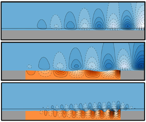

1. Introduction
Taking inspiration initially from the surprising ability of swimming animals to move fast without spending too much energy (Gray Reference Gray1936; Kramer Reference Kramer1961), passive devices have been proposed to postpone the laminar–turbulent transition of boundary layers, based on compliant viscoelastic patches. This paper is motivated by their potentially favourable interaction with the dynamics of laminar boundary-layer flows, which may eventually offer opportunities to decrease the overall drag.
The physics of the flow over compliant walls is rather complex. This paper focuses on the study of low-level disturbances in a boundary layer over a flat plate without adverse pressure gradient, and more specifically on the case where the early stages of the transition to turbulence occur through amplification of the so-called Tollmien–Schlichting waves. At higher disturbance level, this path to turbulence can be bypassed and other mechanisms can be dominant (see Kachanov Reference Kachanov1994), such as the transient growth and breakdown of three-dimensional streak-like structures that can appear in the flow. Within the considered low-disturbance setting, the early stages of the laminar–turbulent transition can be understood by means of the amplification of external small-amplitude perturbations such as acoustic noise, free-stream gusts, etc. Waves generated close to the leading edge are advected by the flow, up to a critical point where an exponential amplification sets in. This exponential growth is well described by the hydrodynamic linear stability theory.
Under the hypothesis of local disturbances, it is possible to study the propagation of travelling waves of type  $A(y)\exp \mathbf {i}(\omega t- kx)$ (where k is the spatial wavenumber) using temporal stability analyses (Tollmien Reference Tollmien1929; Schlichting Reference Schlichting1933) that show that, when the frequency
 $\omega \in \mathbb {R}$ is varied, the boundary layer amplifies waves (
 $k\in \mathbb {C},\ {\rm Im}(k)>0$) in some frequency range; when the Reynolds number based on the displacement thickness is greater than 520. The streamwise position in the flow where the perturbations are amplified also depends on the frequency of the excitation. It is possible to trace the region in the Reynolds number–frequency space where these perturbations are amplified; the line that limits this region – and for which a not-growing and not-decaying perturbation is observed – is called the neutral curve or, very informally, the ‘banana curve’, because of its shape. At some point, it may happen that the linear amplification grows too large in amplitude and triggers nonlinear wave interactions, that eventually result in a fully turbulent flow (Kachanov Reference Kachanov1994). Experiments (Schubauer & Skramstad Reference Schubauer and Skramstad1947) confirmed the existence of these unstable, mainly two-dimensional Tollmien–Schlichting waves.
New effects emerge when the solid wall is deformable with its own elasticity – it is then referred to as an elastic patch/panel, compliant wall or compliant coating. The Tollmien–Schlichting waves (TSW) are affected by the compliance of the wall, and the possibility for waves to travel in the solid favours the emergence of a new class of instabilities, in particular the so-called travelling-wave flutter (TWF).
Thanks to pioneering works by notably Benjamin (Reference Benjamin1960) and Landahl (Reference Landahl1962), it is by now well known that laminar boundary layers over flexible surfaces are susceptible to at least three main types of instabilities. A vast literature is devoted to the study of linear disturbances evolving on a parallel (local analysis), weakly non-parallel or fully streamwise-evolving flow (global analysis) coupled with an infinite or finite-length compliant coating. When the medium is supposed to be of infinite extent in the  $x$ direction, it is convenient to study the propagation of local travelling waves, that allow us in particular to determine the dispersion relation of the coupled solid–fluid problem. However, no account is taken for the ends of the coating in that case. Although some studies have been conducted in three dimensions (Yeo Reference Yeo1992; Lucey & Carpenter Reference Lucey and Carpenter1993), the majority of the approaches deal with two-dimensional geometries, since the instability mechanisms at play at low-amplitude noise level are essentially two-dimensional (Schlichting Reference Schlichting1979). The well-documented series of papers by Carpenter & Garrad (Reference Carpenter and Garrad1985, Reference Carpenter and Garrad1986) and review papers from Gad-El-Hak (Reference Gad-El-Hak1996) and Carpenter, Lucey & Davies (Reference Carpenter, Lucey and Davies2001) cover most of the field between the 1960s and early 2000s.
Travelling-wave analyses coupling one-dimensional wall model with the Orr–Sommerfeld equation (Benjamin Reference Benjamin1960; Landahl Reference Landahl1962; Carpenter & Garrad Reference Carpenter and Garrad1985) characterised the fluid-elastic TSW instability as a slowly convective, downstream-travelling wave in the solid, associated with modified TSW in the fluid. These waves are found to be stabilised by the flexibility of the coating, but destabilised by viscoelastic damping in the solid. Using a more complex model of the solid – the two-dimensional elastic Navier equations – Yeo (Reference Yeo1988) arrived at the same conclusions. Using a weakly non-parallel approximation, Yeo, Khoo & Chong (Reference Yeo, Khoo and Chong1994) also observed that the effects of the boundary-layer growth have only a mild influence on TSW, that increases as the Reynolds number is decreased.
If TSW exist in the rigid case, TWF appears only when the wall is flexible. However, flexibility and damping play a reversed role: decreasing the stiffness of the coating destabilises the TWF, and an increase of damping has a stabilising effect (Benjamin Reference Benjamin1963). TWF is observed as downstream-travelling waves with a velocity close to those of the free-surface waves. As noted by Carpenter & Garrad (Reference Carpenter and Garrad1986), the stabilising effect of damping on TWF is more marked than its destabilising effect on TSW. These are ‘dangerous’ instabilities: as noted by Gad-El-Hak (Reference Gad-El-Hak1996), although the frequency band where the instability occurs is narrower than for the TSW, it extends indefinitely as the Reynolds number increases downstream. It is actually believed that TWF was the main route to transition in the experiments by Gaster (Reference Gaster1988), as reported by Lucey & Carpenter (Reference Lucey and Carpenter1995). The TWF instability is also found to be more sensitive to non-parallel effects than TSW: Yeo et al. (Reference Yeo, Khoo and Chong1994) showed that strong destabilisation can occur due to boundary-layer growth in some TWF regimes.
A third type of instability appears when the pressure fluctuation amplitude outweighs the restoring force due to the stiffness of the coating. Due to this negative added stiffness mechanism, the instability has been identified as a static divergence (SD) instability, well known in aeroelasticity (Dowell Reference Dowell1971). This instability has been observed in water-channel experiments by Gad-El-Hak, Blackwelder & Riley (Reference Gad-El-Hak, Blackwelder and Riley1984) on the form very slow two-dimensional waves normal to the flow, and also on the skin of dolphins and fast human swimmers (Aleyev Reference Aleyev1977). Yeo, Khoo & Zhao (Reference Yeo, Khoo and Zhao1996) showed that the SD appears when the coating is sufficiently soft, but can be suppressed by decreasing the thickness of the coating, hence limiting the effective compliance. TWF and standing wave analyses of the SD instability in infinite panels arrived at the somewhat surprising conclusion that viscoelastic damping is necessary so as to trigger the instability (Landahl Reference Landahl1962; Carpenter & Garrad Reference Carpenter and Garrad1986; Yeo et al. Reference Yeo, Khoo and Zhao1996). The role of damping in finite-length coatings has been studied by Lucey & Carpenter (Reference Lucey and Carpenter1992) using a potential flow approach. They showed in that case that damping is not necessary anymore for triggering the instability. According to them, in infinite-length panels, the energy transfer that leads to divergence is favoured by the slight wave propagation slowdown caused by damping. For finite-length panels, this role is essentially played by edge boundary conditions. In that case, viscoelastic damping only acts as its more classical role of attenuating the growth of the instability. This shows that infinite-length coatings may have a considerably different behaviour than more realistic finite-length coatings – where waves are reflected when they reach the end of the coating.
Another class of instability, referred to as the transitional instability, occurs as a coalescence of TWF and TSW waves. This instability has been documented in particular by Sen & Arora (Reference Sen and Arora1988). In the work by Wiplier & Ehrenstein (Reference Wiplier and Ehrenstein2001), transitional instabilities are also found as a coalescence between an evanescent wave and a Tollmien–Schlichting wave.
Previous theoretical studies have addressed the problem either by assuming an infinite-length coating (Duncan, Waxman & Tulin Reference Duncan, Waxman and Tulin1985; Duncan Reference Duncan1988), or a finite-length coating having a very simple behaviour (spring-backed solid) coupled with inviscid flows (Lucey & Carpenter Reference Lucey and Carpenter1992, Reference Lucey and Carpenter1993) or linearised Navier–Stokes flows (Davies & Carpenter Reference Davies and Carpenter1997; Stewart, Waters & Jensen Reference Stewart, Waters and Jensen2009; Tsigklifis & Lucey Reference Tsigklifis and Lucey2017). On the other hand, the ability of compliant coatings to effectively delay transition in a practically interesting way is still debated (see Luhar, Sharma & McKeon (Reference Luhar, Sharma and McKeon2015) for a review of some of the most recent advances). In particular, it may happen that complex compliant materials (e.g. having a sandwich structure, strong heterogeneities, etc.) would be requested to obtain improved results. These special materials can only be partially modelled using the above-mentioned approaches. For that reason, it is desirable to have at our disposal a framework that can manage a viscous flow as well as a fully elastic, finite-length solid. Such approach may for instance open the way for an advanced optimisation of the structural properties of the coating.
For this reason, we propose here a linearised analysis extended to the case where the coating is modelled as a two-dimensional, finite-length viscoelastic patch. In some sense, this approach is therefore a direct extension of global stability analyses, developed for pure hydrodynamic configurations (Sipp et al. Reference Sipp, Marquet, Meliga and Barbagallo2010; Sipp & Marquet Reference Sipp and Marquet2013a), to the fluid-elastic coupled case.
Due to the special nature of the physical phenomenon at play here (noise-amplifier boundary-layer flow and mode-vibrating solid), two complementary analyses are gainfully employed. The modal analysis allows us to capture self-sustained oscillating phenomenon like TWF. On the other hand, TSW are more naturally analysed in terms of energy amplification of external disturbances. This dual approach was for instance adopted recently by Tsigklifis & Lucey (Reference Tsigklifis and Lucey2017), who performed modal and transient growth analyses for the case of a viscous boundary-layer flow interacting with a finite-length coating modelled by a spring/damper-backed plate equation. In the same spirit, we consider here both modal, eigenvalue fluid-elastic analyses, such as that presented in Pfister, Marquet & Carini (Reference Pfister, Marquet and Carini2019), and an energy-amplification-based approach relying on the resolvent analysis. This second type of approach has been proposed for the case of a pure hydrodynamic laminar boundary-layer flow by Sipp & Marquet (Reference Sipp and Marquet2013a). Within the resolvent framework, introducing a general admittance boundary condition to model a deformable wall, Luhar et al. (Reference Luhar, Sharma and McKeon2015); Luhar, Sharma & McKeon (Reference Luhar, Sharma and McKeon2016) also investigated the means of controlling a turbulent boundary layer through wall viscoelasticity. The basic idea of these approaches is to treat the physical system as a transfer function in frequency space that, given some input forcing, returns an output whose energy can be measured. The mapping between the input and the output is done through the so-called resolvent operator, whose singular value decomposition allows us to identify which forcing causes the most important amplification, and to monitor how the level of amplification varies as a function of the forcing frequency. Similarly to what was done for the modal analysis, we also introduce in this work a fully coupled fluid-elastic resolvent analysis, which will be used in complement to the modal analysis to investigate the problem.
After having introduced the physical modelling in § 2, the decoupled dynamics of the viscoelastic patch and fluid is first analysed in § 3.1, making it possible to identify which vibration modes are likely to interact with the flow. The fluid–solid coupled modes are then determined for different patch stiffness and viscoelastic damping parameters in § 3.2. In the case of sufficient viscoelastic damping, all the modes are stable. The resolvent analysis is then presented and applied in § 4. We first consider the classical rigid-wall case in § 4.1. The fluid-elastic response to an optimal rigid-wall forcing is then calculated and analysed in § 4.2, and finally a fully coupled resolvent analysis is presented in § 4.3. A parametric study is eventually presented in § 4.4. Finally, we investigate in more details the mechanism of TSW attenuation and TWF amplification in § 5.
2. Fluid–solid configuration and equations
2.1. Non-dimensional parameters
The system under study consists in a flat plate in which a rectangular elastic patch of thickness  $H_c^*$ and length
 $L_c^*$ is embedded at a distance
 $L_s^* + L_{w_1}^*$ from the leading edge. The problem is made non-dimensional with respect to the fluid variables, namely the far-field velocity
 $U_\infty ^*$ and the boundary-layer displacement thickness
 $\delta ^*_i$ at the inlet of the computational domain. Non-dimensional variables are noted without the
 $*$ superscript (e.g.
 $H_c = H_c^*/\delta _i^*$, etc.). A sketch of the configuration is reported in figure 1 where non-dimensional lengths have been specified. The incompressible, viscoelastic solid is characterised by its homogeneous density
 $\rho _{s}^*$, Young's modulus
 $E_{s}^*$ (because of the incompressibility constraint, the Poisson ratio is exactly 0.5) and viscoelastic damping coefficient
 $\eta _{s}^*$. The fluid is considered incompressible with a uniform density
 $\rho _{f}^*$ and a dynamic viscosity
 $\nu _f^*$. For a water flow the density is
 $\rho _{f}^*=1000$ kg m
 $^{-3}$ and the dynamic viscosity is approximately
 $\eta _{f}^*=1.00\times 10^{-3}$ Pa s. Four non-dimensional parameters govern the physical properties of the system, namely
 \begin{equation} E_{s} = \frac{E_{s}^*}{\rho_{f}^*\,U^{*2}_\infty},\quad D_{s} = \frac{\eta_{s}^*}{\rho_{f}^*U^{*}_\infty\delta_i^*},\quad M_{s} = \frac{\rho_{s}^*}{\rho_{f}^*}\quad \text{and} \quad Re = \frac{\delta^*_i U_\infty^*}{\nu_f^*} \end{equation}
for the non-dimensional Young's modulus and damping coefficient, solid-to-fluid density ratio and (inlet) Reynolds number respectively. In addition, three geometrical parameters also govern the response of the system, namely
 \begin{equation} L_c = \frac{L_c^*}{\delta_i^*},\quad H_c = \frac{H_c^*}{\delta_i^*},\quad \text{and} \quad L_0 = \frac{L_0^*}{\delta_i^*}=\frac{L_s^*+L_{w_1}^*}{\delta_i^*} \end{equation}
for the non-dimensional length and thickness of the patch, and the position of the patch relative to the leading edge. Physically, the distance  $L_0$ fixes the value of the Reynolds number at the most upstream point of the patch.
Boundary-layer flow over a finite-length compliant coating. Non-dimensional lengths are indicated, the reference length being the boundary-layer displacement thickness at the inflow position. The solid domain  $\Omega _{s}$ is represented in orange colour and the computational fluid domain
 $\Omega _{f}$ in blue colour.

The value of the parameters used for the nominal case are detailed hereafter. For the solid, we consider a stiffness value  $E_{s}=1$, a damping coefficient
 $D_{s}=0.2$ and a density ratio
 $M_{s}=1$. The inlet Reynolds number is fixed to
 $Re=3000$. For this value, TSW developing on the steady boundary-layer flow are found to be convectively unstable (Schmid & Henningson Reference Schmid and Henningson2012; Sipp & Marquet Reference Sipp and Marquet2013b). The non-dimensional length of the patch is set to
 $L_c=100$ and its thickness to
 $H_c = 5$. The choice of the (inlet) Reynolds number fixes the distance
 $L_s=1014$ between the leading edge and the inlet, but we are still free to choose the distance
 $L_{w_1}$, which is fixed to
 $L_{w_1}=25$, which gives
 $L_0 = 1039$. Then, the local Reynolds number based on the boundary-layer thickness evolves over the patch between 3036 and 3179.
Parameters have been chosen so as to be, as much as possible, representative of experimental data. Some dimensional values corresponding to the aforementioned non-dimensional parameters are reported in table 1. They are in the range reported by experiments. For instance, in the experiments by Gad-El-Hak et al. (Reference Gad-El-Hak, Blackwelder and Riley1984) on a laminar boundary layer of inflow velocity 0.2–1.4 m s $^{-1}$, materials having an estimated Young's modulus between 15 and 37 500 Pa have been used. The materials used in Gaster's experiments are found in the same range (Gaster Reference Gaster1988; Lucey & Carpenter Reference Lucey and Carpenter1995). Realistic values of the solid damping coefficient are much harder to determine a priori. For instance, low-stiffness, high damping viscoelastic plastisol gels have damping properties that depend strongly on the temperature or the frequency at which the solid can be loaded (Nakajima, Isner & Harrell Reference Nakajima, Isner and Harrell1981; Nakajima & Harrell Reference Nakajima and Harrell2001). For simplicity, a constant damping coefficient is considered here.
Example of dimensional quantities corresponding to the set of non-dimensional parameters  $E_s=1$,
 $M_s=1$
 $D_s=0.2$,
 $Re=3000$,
 $L_c=100$,
 $H_c=5$ and
 $L_0=1039$.

2.2. Steady Navier–Stokes flow over the rigid configuration
For the range of elastic coefficient  $E_{s}$ explored in this paper, preliminary coupled fluid–solid computations have shown that the steady flow solution comes with only very small-amplitude static deformations of the compliant patch. For instance, for
 $E_s=0.1$ we observed a maximal
 $x$ displacement of
 $1.223\times 10^{-2}$ and a maximal
 $y$ displacement of
 $6.620\times 10^{-7}$ (expressed in non-dimensional units, i.e. relative to
 $\delta _i^*$). Therefore, they will be neglected in the following, and the steady solution of the fluid–solid problem is approximated by a steady boundary-layer flow developing over a rigid wall. It is then described by the steady velocity field
 $\boldsymbol {U}(\boldsymbol {x})$ and pressure field
 $P(\boldsymbol {x})$, that satisfy the incompressible Navier–Stokes equations
 \begin{equation} (\boldsymbol{\nabla}\boldsymbol{U})\boldsymbol{U} - \boldsymbol{\nabla}\boldsymbol{\cdot}\boldsymbol{\sigma}(\boldsymbol{U},P) = 0,\quad \boldsymbol{\nabla}\boldsymbol{\cdot}\boldsymbol{U} = 0 \quad \text{in}\ \Omega_{f}, \end{equation}
where the fluid Cauchy stress tensor is classically defined as  $\boldsymbol {\sigma }(\boldsymbol {U},P) = -P\boldsymbol {I} + 2/Re(\boldsymbol {\nabla }\boldsymbol {U} + {\boldsymbol {\nabla }\boldsymbol {U}}^{\operatorname {T}})$. In these notations,
 $\boldsymbol {\nabla }\boldsymbol {U}$ is the gradient operator that reads
 $\partial U_i/\partial x_j$ in index notation – the advection term
 $(\boldsymbol {\nabla }\boldsymbol {U})\boldsymbol {U}$ thus reads
 $\partial U_i/\partial x_jU_j$ – and
 $\boldsymbol {\nabla }\boldsymbol {\cdot }\boldsymbol {U}$ is the divergence operator. As mentioned before, the computational domain
 $\Omega _{f}$ starts at a non-dimensional distance
 $L_s=L_s^*/\delta _i^*=1014$ from the leading edge of the plate, in such a way that the Reynolds number based on the displacement thickness is
 $3000$ at the inlet, where the flow is modelled by a Blasius profile
 $\boldsymbol {U}_{Blasius}$. This method is relatively common in the literature and comes with very small deviations from a true Navier–Stokes solution over the complete plate (Brandt et al. Reference Brandt, Sipp, Pralits and Marquet2011). As said before, the coating is placed at a non-dimensional distance
 $L_{w_1}=25$ from the inlet. This ensures that the inflow velocity is not influenced by the presence of the coating. The distance between the end of the coating and the outlet is fixed to
 $L_{w_2}=25$. The no-slip velocity condition
 $\boldsymbol {U}=\boldsymbol {0}$ is applied at the undeformed fluid–solid interface
 $\Gamma$. On the top boundary (
 $y=30$), the streamwise velocity is fixed to that of the Blasius flow (the transverse component being left free), while at the outflow boundary (
 $x=L_{w_1}+L_c+L_{w_2}$) the transverse velocity is set to that of the Blasius flow, the streamwise component being left free.
A few features extracted from the solution  $\boldsymbol {Q} = [\boldsymbol {U},P]^{\operatorname {T}}$ to (2.3a,b) are shown in figure 2 as a function of
 $x$. The streamwise-varying displacement thickness
 $\delta ^*(x)$ is represented, as well as the shape factor
 $H$, which allows us to validate the solution with respect to the Blasius theory for a laminar boundary-layer flow: the value slightly oscillates around the theoretical value of
 $2.59$, being fairly stable in the region of interest, i.e. over the viscoelastic patch.
Base solution for the linear analysis. The evolution of the displacement thickness ( $\delta ^*$, solid line (—–)) and the shape factor (
 $H$, dashed line - - -) are reported. The ticks on the
 $x$-axis at the top show the Reynolds number
 $Re_x$ based on the distance from the leading edge.

The computational domain for the fluid region  $\Omega _{f}$ is discretised with a structured mesh made of 72 324 triangles and 36 686 vertices. At the fluid–solid interface, that conforms with the solid mesh, the grid resolution in the streamwise direction is
 ${\rm \Delta} x=0.15$ while the transverse resolution is
 ${\rm \Delta} y^{min}=0.03$. The transverse grid resolution is smoothly decreased in the
 $y>0$ direction using a sine law and reaches
 ${\rm \Delta} y^{max} = 0.3$ close to the upper boundary. The spatial discretisation of the Navier–Stokes equation (2.3a,b) is performed using finite elements and implemented within the software FreeFem++ (Hecht Reference Hecht2012). Lagrange elements
 $P_2$ are considered for the velocity and displacement unknowns, while
 $P_1$ elements are taken to represent the pressure and the interface stress variable. The nonlinear computation of the steady boundary-layer flow from (2.3a,b) is achieved using a Newton method.
2.3. Unsteady linearised arbitrary Lagrangian Eulerian equations governing the fluid–solid perturbations
We are interested in capturing the coupled dynamics of infinitesimal fluid-elastic perturbations developing over the steady pure hydrodynamic flow solution described previously. The unsteady fluid is thus modelled with the viscous linearised Navier–Stokes equations – linearised about the steady boundary-layer flow field. Compliant coatings are often made of rubber or polymer materials (Carpenter & Garrad Reference Carpenter and Garrad1986). The solid is therefore described with an incompressible neo-Hookean viscoelastic model, with a stress–strain relationship taken as being a simple generalisation of the differential Kelvin–Voigt model (Christensen Reference Christensen2012).
The description of the coupled problem can be treated using the formalism presented by Pfister et al. (Reference Pfister, Marquet and Carini2019) and Pfister (Reference Pfister2019). We therefore rely on this approach, which we shall present briefly in the following, and refer the reader to the aforementioned references for a more detailed presentation of the approach, as well as validation studies. The starting point is a formulation of the governing equations using the arbitrary Lagrangian Eulerian (ALE) framework (Hughes, Liu & Zimmermann Reference Hughes, Liu and Zimmermann1981; Donea et al. Reference Donea, Huerta, Ponthot and Rodrigez-Ferran2004). Specifically, the Eulerian fluid equations, naturally expressed in the deformed (by the unsteady fluid–solid deformations) fluid domain are recast in a fixed reference domain  $\Omega _{f}$ by means of a so-called extension operator, introduced so as to propagate the solid interface deformation onto the whole fluid domain. The particular form of this operator is arbitrary, provided that sufficient smoothness is guaranteed – a Laplace equation is used here. On the other hand, the Lagrangian solid equations are kept in their natural form. Once recast in a fixed domain, displacement, velocity and stress interface conditions are easily enforced, and linearisation about a steady flow is straightforward, although quite tedious.
For conciseness of the notations, the fluid-elastic perturbations are split into two groups of variables. The first group  $\boldsymbol {q}_{s}'$ regroups the elastic solid displacement field (extended to the fluid domain because of the ALE formulation), a displacement velocity variable used to formulate the elasticity equation first order in time and the solid pressure (introduced because the neo-Hookean solid model is incompressible). The second group of variables
 $\boldsymbol {q}_{f}'$ regroups the Eulerian fluid velocity recast in the fixed domain, the fluid pressure and a Lagrange multiplier variable that represents the interface stress. The governing equations then take the block-operator form
 \begin{equation} \begin{pmatrix} \boldsymbol{\mathsf{B}}_{s} & \boldsymbol{\mathsf{0}} \\ \boldsymbol{\mathsf{0}} & \boldsymbol{\mathsf{B}}_{f} \end{pmatrix} \frac{\partial}{\partial t} \begin{pmatrix} \boldsymbol{q}_{s}' \\ \boldsymbol{q}_{f}' \end{pmatrix}- \begin{pmatrix} \boldsymbol{\mathsf{A}}_{s} & \boldsymbol{\mathsf{C}}_{sf} \\ \boldsymbol{\mathsf{C}}_{fs} & \boldsymbol{\mathsf{A}}_{f}(\boldsymbol{Q}) \end{pmatrix} \begin{pmatrix} \boldsymbol{q}_{s}' \\ \boldsymbol{q}_{f}' \end{pmatrix} = \begin{pmatrix} \boldsymbol{0} \\ \boldsymbol{\mathsf{P}}_{f}\boldsymbol{f}' \end{pmatrix}. \end{equation}
In this notation,  $(\boldsymbol{\mathsf{B}}_{s},\boldsymbol{\mathsf{A}}_{s})$ represent the linearised solid-extension operators that only depend on the material parameters
 $D_{s}$,
 $M_{s}$ and
 $E_{s}$. The fluid operators
 $(\boldsymbol{\mathsf{B}}_{f},\boldsymbol{\mathsf{A}}_{f})$ regroup the linearised Navier–Stokes equations, that depend on the pure hydrodynamic steady flow
 $\boldsymbol {Q} = [\boldsymbol {U},P]^{\operatorname {T}}$ and on the Reynolds number. The off-diagonal operators
 $\boldsymbol{\mathsf{C}}_{sf}$ and
 $\boldsymbol{\mathsf{C}}_{fs}$ are the coupling operators, which take into account how the infinitesimal deformation of the fluid–solid interface affects the flow, and vice versa. These terms reflect the chosen two-way coupling approach. Finally, the right-hand side term accounts for an external distributed forcing in the fluid momentum equation, the operator
 $\boldsymbol{\mathsf{P}}_{f}$ being introduced to adjust the dimension of the vector, i.e.
 $\boldsymbol{\mathsf{P}}_{f}\boldsymbol {f}' = [\boldsymbol {f}',\boldsymbol {0},\boldsymbol {0}]^{\operatorname {T}}$. The elasticity problem can again be decomposed between the solid and extension variables in the following way:
 \begin{equation} \boldsymbol{\mathsf{A}}_{s} = \begin{pmatrix} \boldsymbol{\mathsf{A}}_{ss} & \boldsymbol{0} \\ \boldsymbol{\mathsf{C}}_{es} & \boldsymbol{\mathsf{A}}_{ee} \end{pmatrix} \quad \text{and} \quad \boldsymbol{\mathsf{B}}_{s} = \begin{pmatrix} \boldsymbol{\mathsf{B}}_{ss} & \boldsymbol{0} \\ \boldsymbol{0} & \boldsymbol{0} \end{pmatrix}. \end{equation}
The operator  $\boldsymbol{\mathsf{A}}_{ss}$ corresponds to the elasticity problem, while
 $\boldsymbol{\mathsf{A}}_{ee}$ corresponds to the extension problem – the block-triangular structure of
 $\boldsymbol{\mathsf{A}}_{s}$ reflects the fact that the extension problem is entirely subordinated to the solid problem. Detailed equations are reported in Appendix A.
The different fluid–solid operators involved in (2.4) are also modelled via finite elements and implemented within the software FreeFem++ (Hecht Reference Hecht2012). The extension region is made as a layer (of non-dimensional width of  $5$) of cells around the compliant patch. The computational domain of the solid region is discretised with a structured mesh made with 17 982 triangles and 9352 vertices. The eigenvalue and resolvent computations are handled with the eigenvalue library ARPACK (Lehoucq, Sorensen & Yang Reference Lehoucq, Sorensen and Yang1997) which is based upon an algorithmic variant of the Arnoldi process called the implicitly restarted Arnoldi method. The use of a shift-and-invert strategy enables eigenvalues to be obtained in the vicinity of a given complex shift. The numerical computation of the singular values in the global resolvent analysis (§ 4) is based on the reformulation of the singular value problem as an eigenvalue problem (Sipp & Marquet Reference Sipp and Marquet2013b). The direct sparse lower–upper (LU) solver multifrontal massively parallel sparse direct solver (MUMPS) (Amestoy et al. Reference Amestoy, Buttari, Guermouche, L'Excellent and Ucar2013) is used for all matrix inverse operations needed by the algorithms.
3. Eigenvalue analysis
We investigate in this section the long-term stability of the boundary-layer flow interacting with the compliant patch. The eigenvalue analyses of the decoupled fluid and solid problems are first performed in § 3.1. The computation of the solid modes in absence of fluid – in vacuo modes – allows for an estimation of the characteristic frequencies of the isolated patch, and by comparison with the purely fluid spectrum, the identification of a range of stiffness values that are likely to result in a strong interaction between the patch and the fluid. The eigenvalue analysis of the coupled fluid–solid problem is then presented in § 3.2.
3.1. Decoupled eigenvalue analysis
The purely fluid eigenvalue problem is obtained by considering only the fluid operator in (2.4). Modes are sought on the form
 \begin{equation} \boldsymbol{q}_{f}'(\boldsymbol{x},t)=\boldsymbol{q}_{{f}}^\circ(\boldsymbol{x})\exp\left((\lambda^r + \mathbf{i}\lambda^i)t\right) \end{equation}
with damping  $\lambda ^r$ and circular frequency
 $\lambda ^i$, resulting in the eigenvalue problem
 \begin{equation} \left\{(\lambda^r + \mathbf{i}\lambda^i)\boldsymbol{\mathsf{B}}_{f}-\boldsymbol{\mathsf{A}}_{f}(\boldsymbol{Q})\right\}\boldsymbol{q}_{{f}}^\circ{=}\boldsymbol{0}, \end{equation}
where  $\boldsymbol {Q} = [\boldsymbol {U},P]^{\operatorname {T}}$ is the fluid steady flow (cf. § 2.2). For the steady flow as well as for the perturbation problem, no-slip boundary conditions are considered at the wall (patch included). The obtained fluid spectrum is reported by the open diamonds in figure 3; it reveals the branch of modes responsible for the TSW (Ehrenstein & Gallaire Reference Ehrenstein and Gallaire2005; Åkervik et al. Reference Åkervik, Ehrenstein, Gallaire and Henningson2008) and, hence, the frequencies of interest of the fluid instability, ranging between
 $0.02$ and
 $0.1$.
Decoupled eigenvalue analysis. Two in vacuo spectra are reported for the solid: a case without ( $D_{s}=0$, orange circles
 $\circ$, orange) and a case with viscoelastic damping (
 $D_{s}=0.2$, orange squares
 $\square$, orange). The fluid spectrum (blue diamonds
 $\lozenge$, blue) is also reported as a reference. The insets at the bottom represent the
 $y$ displacement component of eight representative solid in vacuo modes, highlighted in black and marked
 $1,2,\ldots,8$ in the figure on top. Dashed contours indicate negative values.

Similarly, in vacuo solid modes are obtained by considering only the solid operator. Looking for modes on the form  $\boldsymbol {q}_{s}'(\boldsymbol {x},t) = \boldsymbol {q}_{s}^\circ (\boldsymbol {x})\exp ((\lambda ^r + \mathbf {i}\lambda ^i)t)$ in (2.4), we obtain the solid eigenvalue problem
 \begin{equation} \left\{(\lambda^r + \mathbf{i}\lambda^i)\boldsymbol{\mathsf{B}}_{s}-\boldsymbol{\mathsf{A}}_{s}(E_{s},D_{s})\right\}\boldsymbol{q}_{s}^\circ{=}\boldsymbol{0}. \end{equation}
This problem is a combined elastic–extension vibration problem, that is strictly equivalent to an elastic-only problem, since the extension problem is entirely subordinated to the elastic one. The only component of interest in  $\boldsymbol {q}_{s}^\circ$ is thus the solid displacement
 ${\boldsymbol {\xi }^\circ }$. A zero-displacement boundary condition is prescribed at the bottom and side edges of the viscoelastic patch, while – in the absence of the surrounding fluid – a stress-free condition is applied on the upper side of the patch.
Spectrum and mode shapes solution to (3.3) for  $E_{s}=1$ and
 $D_{s}=0$, and the nominal geometry for which
 $L_c=100$ and
 $H_c=5$, are reported by the open circles in figure 3. As there is no damping or coupling with the fluid, no temporal growth or decay process is involved: all modes are neutrally stable (
 $\lambda ^r=0$). The free-vibration eigenvalues for a non-zero damping coefficient are also reported by the open squares in figure 3. In presence of damping, the eigenvalues are no longer imaginary as is the case when
 $D_{s}=0$ but present a negative growth rate, i.e. they are akin to damped oscillations. The higher the frequency, the more negative the growth rate is, as is traditionally observed for damped linear oscillators. The decay of the growth rate can be for instance evaluated as
 $\lambda ^r = -3D_{s}/(2E_{s})(\lambda ^i_0)^2$, where
 $\lambda ^i_0$ is the frequency of the modes without damping. Interestingly, note that all modes are located above a threshold frequency of approximately
 $\lambda ^i=0.18$. In the bottom part of figure 3, eight modes shapes are represented in increasing order in terms of their frequency. The
 $y$ displacement is shown together with the interface deformation for a better visualisation. This zoology of modes shows the great variety of modal behaviours that can be found. Because the length of the coating is finite, the admissible streamwise wavelengths are actually
 $L_c^*$,
 $L_c^*/2, \ldots, L_c^*/n$, …, with
 $n \in \mathbb {N}$, which results in a great variety of patterns.
To better understand what is the physical origin of the solid modes, and also explain the presence of a low-frequency cutoff, it is useful to relate these modes to those that can be calculated for a patch of infinite length. In this latter case, results have been obtained with a travelling-wave analysis notably by Duncan et al. (Reference Duncan, Waxman and Tulin1985) and Gad-El-Hak et al. (Reference Gad-El-Hak, Blackwelder and Riley1984), by looking in the linearised Navier elasticity equation for waves that travel freely in the horizontal  $x$ direction – there are no side edges anymore in this case. We then consider the same elasticity equation as before, but now discard the side edges boundary condition, and search for travelling waves in the form of a streamfunction
 $\phi (x,y,t) = \hat {\phi }(y)\exp (\lambda t - \mathbf {i} k x)$, such that
 \begin{equation} [\boldsymbol{\xi'}_\infty]_x= \frac{\partial \phi}{\partial y} = \underbrace{\left(\frac{\mathrm{d}\hat{\phi}}{\mathrm{d} y}{\rm e}^{-\mathbf{i} k x}\right)}_{[\boldsymbol{\xi}_\infty^\circ]_x} {\rm e}^{\lambda t}\quad \text{and}\quad [\boldsymbol{\xi'}_\infty]_y={-}\frac{\partial\phi}{\partial x} = \underbrace{\left(\mathbf{i} k \hat{\phi}(y)\,{\rm e}^{-\mathbf{i} k x}\right)}_{[\boldsymbol{\xi}_\infty^\circ]_y}{\rm e}^{\lambda t}, \end{equation}
where again  $\lambda = \lambda ^r + \mathbf {i}\lambda ^i$, and the displacement is noted
 $\boldsymbol {\xi }_\infty$ to mark the difference from the finite-length case. Note also that, for consistency with the rest of the paper, the original non-dimensionalisation is kept, even if it is not the most appropriate for a solid-based analysis. Based on this decomposition, it can be shown that, for each value of
 $k\in \mathbb {R}$, solving an eigenvalue problem gives the corresponding values of
 $\lambda \in \mathbb {C}$, which eventually allows us to reconstruct the dispersion relation in the
 $(k,\lambda )$ plane but also to compute mode shapes. The reader is referred to Appendix C for the technical details, including the precise form of the obtained equations.
For the case  $E_s=M_s=1$ and
 $D_s=0$, the dispersion relation is reported in figure 4(a) with black curves. We observe that it is composed of several branches of increasing frequency, and each branch is marked with a frequency cutoff at low wavenumbers (i.e. large spatial wavelengths in the
 $x$ direction). In this limit, everything happens as if the coating was experiencing a bulk displacement over its whole length, and the frequency limit of each branch thus corresponds to the different natural frequencies for this transverse movement. The material is strongly dispersive for small
 $k$: waves having different wavenumbers can share almost the same frequency. On the other hand, at larger values of
 $k$ (i.e. smaller spatial wavelengths in the
 $x$ direction) the lowest-frequency branch asymptotically reaches the non-dispersive dispersion relation established by Rayleigh (Reference Rayleigh1885) for a semi-infinite medium (represented by the red dashed line). Note that, because the material is incompressible, there is only one finite characteristic wave speed associated with the problem (that of shear waves). In the case of a compressible material, one would also have a characteristic velocity associated with dilatational waves (its velocity scales with
 $1/\sqrt {1-2\nu )}$ where
 $\nu$ is the Poisson coefficient of the material) which would modify the distribution of the solid eigenfrequencies and also introduce new type of modes. This case is not considered in this study, but would certainly deserve further investigation. Mode shapes are reported in figure 4(b), for each branch
 $a$,
 $b$ and
 $c$ and two values of
 $k$. We observe that the number of transverse vibration nodes of the mode shape increases when we go from branch
 $a$ to branch
 $b$ then
 $c$. The wavenumber
 $k$ has also a noticeable influence on the form of the modes, especially for those located on branch
 $b$.
Infinite-length patch for the case  $E_s=M_s=1$ and
 $D_s=0$. (a) Dispersion relation (black lines), Rayleigh's dispersion relation for a semi-infinite (red dashed line) and modes of the finite-length patch (colour circles and black crosses to mark the representative modes displayed in figure 3). The three lowest frequency branches are labelled
 $a,b,c$. (b) Real part of the
 $y$ displacement of the mode shapes for
 $k=0.1$ (black solid line) and
 $k=2$ (dashed line), for modes located on branches
 $a$ (left),
 $b$ (middle) and
 $c$ (right).

The infinite-length mode shapes  $\boldsymbol {\xi }_\infty ^\circ$ can be used as a projection basis to evaluate what is the ‘infinite-length content’ of the finite-length modes
 ${\boldsymbol {\xi }^\circ }$. Specifically, we introduce a modal assurance criterion
 \begin{equation} \text{MAC}({\boldsymbol{\xi}^\circ};k,\alpha) = \frac{|\left\langle\boldsymbol{\xi}_{\infty,\alpha}^{{\circ}}(k), {\boldsymbol{\xi}^\circ}\right\rangle|}{\|\boldsymbol{\xi}_{\infty,\alpha}^\circ(k)\|\,\|{\boldsymbol{\xi}^\circ}\|}\quad |\alpha\in\{a,b,c\}, \end{equation}
where  $\langle \cdot,\cdot \rangle$ is the standard scalar product on the finite-length solid displacement space and
 $\|\cdot \|$ the associated norm. For a given mode
 ${\boldsymbol {\xi }^\circ }$, calculating
 $\operatorname {argmin}_{k,\alpha } \text {MAC}({\boldsymbol {\xi }^\circ };k,\alpha )$ allows us to evaluate to which infinite-length branch of modes
 $\alpha$, and to which wavenumber
 $k$ this mode is most closely related. This exercise has been done for the in vacuo modes presented in figure 3. This then allows each mode – whose best
 $k$ and
 $\alpha$ values have been calculated – to be superimposed on the dispersion relation: the frequency (as obtained from (3.3)) gives the
 $y$-ordinate and the estimated
 $k$ value gives the
 $x$-ordinate. Points with
 $\alpha =a$ are represented in red colour, those with
 $\alpha =b$ in green colour and those
 $\alpha =c$ in blue colour. As can be seen in figure 4(a), an excellent match is found : finite-length modes are essentially infinite-length modes of type
 $a$,
 $b$ or
 $c$ ‘truncated’ at some value of
 $k$ compatible with the boundary conditions. In particular, the representative modes
 $(1),\ldots,(8)$ shown in figure 3 have been highlighted on the graph, showing that modes
 $(1)$,
 $(2)$ and
 $(4)$ are mostly related to branch
 $a$, modes
 $(3)$ and
 $(5)$ to branch
 $b$ and modes
 $(6)$,
 $(7)$ and
 $(8)$ to branch
 $c$.
The solid vibration frequencies can be tuned mainly by changing the Young's modulus and/or the density of the material, since the frequency scales as  $\sqrt {E_s/M_s}$. Apart from the material constants, the geometry also influences the vibration frequencies. Especially, the effect of changing the length of the patch is represented in figure 5, where the patch vibration frequencies
 $\lambda ^i$ are reported as a function of
 $L_c$ (for the case
 $H_c=5$ and
 $D_s=0$). For a given value of
 $L_c$, each point in the graph corresponds to a modal vibration frequency. As the geometry is modified, we observe that these frequencies also evolve on branches. As exposed above, these branches are related to the branches observed in the infinite-length coating: adding side boundary conditions essentially amounts to constraining the admissible values for the spatial wavenumber in the
 $x$ direction. In order to facilitate the reading of the figure, each point on the graph is also coloured according to the branch of infinite modes on which its projection is the largest. We observe that lowest-frequency modes are related to infinite-length branch
 $a$, then branch
 $b$ and branch
 $c$. The region where these different mode types are found overlap, meaning that at a given frequency several modes of different type can be found. For the sake of comparison, the three lowest frequencies (in the limit of a zero longitudinal wavenumber, i.e.
 $k \to 0$) computed with the travelling-wave analysis are reported with a dashed line (see figure 4). Now the influence of the length of the patch can be assessed: for low aspect ratios, the cutoff frequency tends to move higher. For instance, for the extreme case where
 $L_c=1$ the lowest frequency is found slightly below
 $0.75$. However, as
 $L_c$ increases the lowest frequency quickly reaches its absolute minimum, meaning that the length of the patch as only a mild influence on the lowest frequency it can carry as long as
 $L_c/H_c\gtrsim 10$. Finally, the frequency of the modes is also related to the thickness
 $H_c$ of the coating: increasing the thickness decreases the vibration frequencies, which evolve as
 $1/H_c$.
Evolution of in vacuo solid vibration frequencies as a function of  $L_c/H_c$ (for
 $H_c=5$), for the case
 $E_s=1$ and
 $D_s=0$. Each point is coloured according to the branch of infinite modes on which its projection is the largest (red for branch
 $a$, green for branch
 $b$ and blue for branch
 $c$). The three lowest frequencies when
 $k \to 0$ computed with the travelling-wave analysis are represented with a dashed line (cf. figure 4a).

3.2. Coupled eigenvalue analysis
Let us now move on the coupled analysis. For that purpose, the fluid and solid variables are decomposed on the form of a coupled fluid-elastic global mode, i.e.
 \begin{equation} \begin{pmatrix}\boldsymbol{q}_{s}' \\ \boldsymbol{q}_{f}' \end{pmatrix}(\boldsymbol{x},t) =\begin{pmatrix} \boldsymbol{q}_{s}^\circ \\ \boldsymbol{q}_{{f}}^\circ \end{pmatrix}\!\!(\boldsymbol{x}) \exp\left((\lambda^r + \mathbf{i}\lambda^i)t\right) \end{equation}
where again  $\lambda ^r$ is the growth rate and
 $\lambda ^i$ is the angular frequency. Injecting that ansatz in the linearised problem (2.4) – without any forcing term – gives the eigenvalue problem
 \begin{equation} \left\{(\lambda^r + \mathbf{i}\lambda^i) \begin{pmatrix} \boldsymbol{\mathsf{B}}_{s} & \boldsymbol{\mathsf{0}} \\ \boldsymbol{\mathsf{0}} & \boldsymbol{\mathsf{B}}_{f} \end{pmatrix}- \begin{pmatrix} \boldsymbol{\mathsf{A}}_{s}(E_{s},D_{s}) & \boldsymbol{\mathsf{C}}_{sf} \\ \boldsymbol{\mathsf{C}}_{fs} & \boldsymbol{\mathsf{A}}_{f}(\boldsymbol{Q}) \end{pmatrix} \right\} \begin{pmatrix} \boldsymbol{q}_{s}^\circ \\ \boldsymbol{q}_{{f}}^\circ \end{pmatrix}= \boldsymbol{0}. \end{equation}
First, we consider a case without viscoelastic damping ( $E_{s}=1$ and
 $D_{s}=0$). The eigenvalue spectrum of the fully coupled, linearised fluid–solid operators is displayed in figure 6, while a few representative eigenvectors are reported in figure 7. The spectrum is described in the following. Although resulting from a fully coupled analysis, one still finds the trace of the decoupled modes (solid and fluid) in this spectrum.
Coupled eigenvalue analysis. The spectra of the coupled fluid-structural system for a purely elastic wall ( $D_{s}=0$) are reported by open circles (
 $\circ$), and the ones for a viscoelastic wall (
 $D_{s}=0.2$) by open squares (
 $\square$). The elasticity coefficient is
 $E_{s}=1$ in both cases. The labelled modes highlighted in red are reported in figure 7.

Mode shapes corresponding the eigenvalues labelled (a–d) in figure 6. Dashed contours indicate negative values.

The stable ensemble of modes the closest to the real axis is clearly related to the TSW and it can also be found in the rigid-wall spectrum (cf. figure 3). The eigenvector corresponding to the most unstable of these modes is reported in figure 7(a). The exponential growth along the streamwise direction causes the localisation of the perturbation in the outflow region.
Although the individual two-dimensional modes are stable, an appropriate superposition of them may exhibit a transient growth (Ehrenstein & Gallaire Reference Ehrenstein and Gallaire2005); the dynamics of the TSW has indeed more to do with receptivity and energy-amplification mechanisms than modal behaviour (Schmid Reference Schmid2007). For that reason, a resolvent analysis is performed in § 4.
Unstable modes can be found in figure 6 at frequencies above  $0.35$; figure 7(b) reports the mode at lowest frequency related to this ‘branch’ of modes, and figure 7(c,d) the first (when the stiffness increases) and the most unstable ones. These modes are clearly related to the destabilisation of the free-vibration solid modes (cf. figure 3) via the interaction with the fluid. In the following, we refer to these modes as the TWF modes. Note that the frequency of the coupled modes is slightly shifted towards lower frequencies because of added mass effects, compared with in vacuo frequencies. This part of the spectrum is in qualitative agreement with what was observed in the global mode analysis by Tsigklifis & Lucey (Reference Tsigklifis and Lucey2017) in the case without damping: one branch of unstable modes was found in approximately the same frequency range. In the present case, more than one branch of structural modes is observed, as reported in figure 6: a second branch of structural modes is found at frequencies higher than approximately
 $0.5$, since our solid model enables to carry many more types of modes than the spring-backed solid considered by Tsigklifis & Lucey. We observe ‘discontinuities’ in the arrangement of modes as the frequency increases. These slope breaks are probably related to the transition from one type of solid mode to another (cf. figure 4), but quantitatively it is difficult to clearly associate the solid component of each coupled modes with one or the other branch of in vacuo solid modes (for instance using projection on the modal basis as was done in § 3.1), as the modes shapes are strongly impacted by the fluid–structure coupling.
It is well known that the eigenvalues related to the TSW are sensitive to the location and type of boundary conditions considered (Ehrenstein & Gallaire Reference Ehrenstein and Gallaire2005). We also observed this phenomenon by varying the distance between the end of the coating and the outflow. With the chosen dimensions for the domain, the region that drives the instability is indeed not completely covered by the computational grid. This is, however, not really an issue, because we are rather interested by the effect of variations of the material parameters than by the absolute values. On the other hand, the eigenvalues related to the solid-based instabilities are completely insensitive to the dimensions of the domain. In that case, the region that drives the instability is indeed located in the vicinity of the patch.
The presence of these unstable modes obviously excludes the possibility of controlling the flow with a purely elastic patch. As one can see from the eigenvalues reported for the case  $D_{s}=0.2$ in figure 6, conferring a viscous behaviour to the material adds sufficient damping so that the TWF modes are eventually stable. On the other hand, the TSW branch remains mostly unchanged.
Let us now investigate the effect of varying the parameters in a more general way. In particular, it is interesting to investigate what happens when the stiffness is decreased: in this case TWF modes are shifted towards lower frequencies, and our fully coupled approach would then allow us to capture (if any) a merging of TWF and TSW modes. Spectra for  $E_s=0.5$,
 $E_s=0.25$ and
 $E_s=0.1$, with and without damping, are reported in figure 8(a). It can be seen that the lowest TWF frequency decreases with
 $Es$, up to the point it reaches the TSW mode region. However, this does not lead to a destabilisation of the TWFs in this region: there is finally little interaction there. On the other hand, modes become very unstable at higher frequencies (between
 $0.2$ and
 $0.3$), and we observe in particular that damping has little effect on these modes. A quite similar behaviour can be observed when the thickness of the patch is increased, as reported in figure 8(b). There are some important differences, however. Specifically, the magnitude of
 $\lambda ^r$ does not increase with the increase in thickness, unlike the case of decreasing stiffness. Moreover, it seems that the frequency at which the TWF modes become unstable seems to decrease as
 $2/H_c$ when the patch is sufficiently thick. Finally, note that we do not observe any low- or zero-frequency unstable eigenvalues (divergence modes). Specifically, all zero-frequency modes visible in figure 8 have a negative growth rate. Using potential flow calculations and a travelling-wave analysis, Duncan et al. (Reference Duncan, Waxman and Tulin1985) could determine a (conservative) estimate for the threshold of divergence, which was found to occur for flow speeds
 $U_\infty ^* = 2.86C_T$, where
 $C_T = \sqrt {E_s^*/3\rho _s^*}$ is the velocity of elastic shear waves. Translated to the notations of the present study, this gives a threshold at
 $E_s=0.37$. Obviously, no such instability is observed in the range of stiffnesses covered in the study: divergence should happen at lower stiffness values and the estimate by Duncan et al. (Reference Duncan, Waxman and Tulin1985) can indeed be considered very conservative.
Effect of (a–f) decreasing the stiffness and (g–j) increasing the thickness of the patch on the fluid–solid coupled eigenmodes.

This effect of viscosity and stiffness on the stability properties of the coupled system is now investigated in a more systematic manner. By looking for the eigenvalues of largest real part for different values of the stiffness  $E_{s}$ and damping
 $D_{s}$, we can determine the region in this parameter space where the configuration is globally stable or unstable.
The influence of the stiffness  $E_{s}$ and the viscoelastic damping
 $D_{s}$ on the most unstable eigenvalues
 $\lambda _{cr}$ is reported in figure 9. From the real part of
 $\lambda _{cr}$ (figure 9a), one can identify the regions in the parameter space for which the system is unstable (red shade) and stable (blue shade). The dashed line indicates the border between these two regions, i.e. the critical boundary. The rigid-wall limit is recovered there, with the system becoming stable for large values of
 $E_{s}$: in this limit the patch does not interact with the fluid and the two systems behave as decoupled, with the solid modes being stable or neutrally stable depending on the viscosity term. The imaginary part of the most unstable eigenvalue is also reported in figure 9(b), scaled by the square root of Young's modulus
 $E_{s}$. Thanks to this scaling, it is possible to identify where in the TWF branch is located
 $\lambda _{cr}$: an orange shade indicates an eigenvalue of the type (d) in figure 7, while a green shade an eigenvalue of the type (a).
Influence of the viscoelastic damping  $D_{s}$ and stiffness
 $E_{s}$ on the fully coupled fluid–solid spectrum. (a) Reports the real part of the most unstable eigenvalue
 $\lambda _{cr}$, and (b) its rescaled imaginary part: the dashed lines separate the stable and unstable regions of the parameter space. The imaginary part has been scaled with the solid quantities, i.e. by the square root of Young's modulus
 $E_{s}$. The crosses indicate the combinations of
 $(E_{s}, D_{s})$ for which the spectrum has been computed.

The combined information given by the two figures tells us the stabilisation scenario is by the material's viscosity. Let us consider a fixed Young's modulus, e.g.  $E_{s}=1$: (i) without viscosity (
 $D_{s}=0$) the system is unstable (red shade in figure 9a), with the most growing mode of the type (d) (orange shade in figure 9b); (ii) increasing
 $D_{s}$, the system becomes neutrally stable (white contour in figure 9a), with the mode of type (d) still being the closest to the imaginary axis; (iii) further increasing the viscosity pushes the eigenvalues deeper in the stable region (blue shade in figure 9a), letting the mode of type (a) be the closest to the imaginary axis (green shade in figure 9b).
In the following, we consider a globally stable case ( $E_{s}=1$ and
 $D_{s}=0.2$), and consider the resolvent analysis.
4. Resolvent analysis
The development of the TSW in boundary-layer flows is conveniently analysed in terms of the receptivity of the flow to external perturbations (Schmid Reference Schmid2007). Even in linearly stable systems, strong energy amplifications may indeed occur because of the transient energy growth provoked by the non-normality of the linearised Navier–Stokes operator. We first apply a resolvent analysis in the rigid-wall configuration. This allows us to determine which perturbation in the flow leads to the strongest response of the flow, independently of any elasticity effect. Then, considering this optimal, rigid-wall perturbation, the response in the viscoelastic case is computed and analysed. Finally, the optimal forcings and their responses are computed for the coupled fluid–viscoelastic system. This two-stage approach allows us in particular to dissociate one-way coupling effects from two-way coupling effects in the fluid–solid dynamics. Unless otherwise stated, we consider here the globally stable case  $E_{s}=1$ and
 $D_{s}=0.2$ identified in § 3.
4.1. Resolvent analysis in the rigid-wall case
In our framework, the governing equations for the fluid velocity and pressure perturbation  $\boldsymbol {q}_{f}'$ developing about the boundary-layer flow past a rigid wall, and excited by some momentum forcing
 $\boldsymbol {f}'$, corresponds to the subproblem
 \begin{equation} \boldsymbol{\mathsf{B}}_{f}\frac{\partial \boldsymbol{q}_{f}'}{\partial t} - \boldsymbol{\mathsf{A}}_{f}\,\boldsymbol{q}_{f}' = \boldsymbol{\mathsf{P}}_{f}\,\boldsymbol{f}', \end{equation}
deduced from (2.4). In the linear framework, the response to a generic forcing akin to free-stream perturbations (gusts, etc.) can be computed as the sum of independent responses to each harmonic component of the original forcing, thanks to the superposition principle. Hence, we assume a harmonic forcing
 \begin{equation} \boldsymbol{f}'(\boldsymbol{x},t) = \boldsymbol{f}(\boldsymbol{x})\,{\rm e}^{\mathbf{i}\omega t} + \mbox{c.c.} \end{equation}
where c.c. stands for the complex conjugate. Because of the linearity of (4.1), this harmonic forcing leads to a harmonic fluid response
 \begin{equation} \boldsymbol{q}_{f}'(\boldsymbol{x},t) = \boldsymbol{\hat{q}}_{{f}}(\boldsymbol{x})\,{\rm e}^{\mathbf{i}\omega t} + \mbox{c.c.}, \end{equation}
where the state  $\boldsymbol {\hat {q}}_{{f}}(\boldsymbol {x})$ represents a fluid pressure–velocity mode. Introducing the fluid resolvent operator
 $\boldsymbol{\mathsf{R}}_{f}(\omega ) = (\mathbf {i}\omega \boldsymbol{\mathsf{B}}_{f}-\boldsymbol{\mathsf{A}}_{f})^{-1}$, the fluid response
 $\boldsymbol {\hat {q}}_{{f}}$ to a momentum forcing
 $\boldsymbol {f}(\boldsymbol {x})$ reads, in the rigid configuration, is
 \begin{equation} \boldsymbol{\hat{q}}_{{f}} = \boldsymbol{\mathsf{R}}_{f}(\omega)\boldsymbol{\mathsf{P}}_{f}\boldsymbol{f}. \end{equation}
The TSW developing in the rigid-wall configuration can be characterised by varying the frequency  $\omega$ and by looking for the spatial distribution of
 $\boldsymbol {f}(\boldsymbol {x})$ that gives the greatest amplification
 $G(\omega )$ of the fluid velocity perturbations
 $\boldsymbol {u}_{{f}}(\boldsymbol {x})$ – extracted from
 $\boldsymbol {\hat {q}}_{{f}}(\boldsymbol {x})$ – akin to these unstable waves (Sipp & Marquet Reference Sipp and Marquet2013b). Namely, we set
 \begin{equation} \left.\begin{gathered} \displaystyle \sigma^2_0(\omega) = \max_{\|\boldsymbol{f}\|^2=1}\|\boldsymbol{u}_{{f}}\|^2 \quad \text{with} \displaystyle \|\boldsymbol{f}\|^2 = \int_{\Omega_{f}}|\boldsymbol{f}|^2\,\mathrm{d}\varOmega = \left\langle\,\boldsymbol{f}, \boldsymbol{f}\right\rangle = \boldsymbol{f}^{{{\dagger}}}\boldsymbol{\mathsf{Q}}_f\boldsymbol{f},\\ \displaystyle \|\boldsymbol{u}_{{f}}\|^2 = \int_{\Omega_{f}}|\boldsymbol{u}_{{f}}|^2\,\mathrm{d}\varOmega = \left\langle\boldsymbol{\hat{q}}_{{f}}, \boldsymbol{\hat{q}}_{{f}}\right\rangle_u = \boldsymbol{\hat{q}}_{{f}}^{{{\dagger}}}\boldsymbol{\mathsf{Q}}_{{f}u}\boldsymbol{\hat{q}}_{{f}}, \end{gathered}\right\} \end{equation}
the perturbation kinetic energy measured over the whole fluid domain, normalised by the forcing energy. The matrices  $\boldsymbol{\mathsf{Q}}_f$ and
 $\boldsymbol{\mathsf{Q}}_{{f}u}$ correspond to the discrete operators used to compute the spatial norms over the fluid computational domain. Using (4.4) and the adjoint resolvent operator
 $\boldsymbol{\mathsf{R}}_{f}(\omega )^{\dagger}$ – which corresponds numerically to the Hermitian transpose of
 $\boldsymbol{\mathsf{R}}_{f}(\omega )$) – the solutions to this constrained optimisation problem can be obtained by solving the generalised eigenvalue problem (Brandt et al. Reference Brandt, Sipp, Pralits and Marquet2011)
 \begin{equation} \left(\boldsymbol{\mathsf{P}}_{f}^{\operatorname{T}}\boldsymbol{\mathsf{R}}_{f}(\omega)^{{{\dagger}}}\boldsymbol{\mathsf{Q}}_{{f}u}\boldsymbol{\mathsf{R}}_{f}(\omega)\boldsymbol{\mathsf{P}}_{f}\right)\boldsymbol{f} = \sigma^2\boldsymbol{\mathsf{Q}}_f\boldsymbol{f}. \end{equation}
The eigenvalues  $\sigma ^2_0>\sigma ^2_1>\cdots$ are positive since the left- and right-hand sides of this problem are Hermitian. In the present case, the explicit form of the adjoint resolvent operator does not need to be determined: the discrete adjoint approach is considered. Once the forcing field is determined, the velocity perturbation response can by computed using (4.4). The triplet
 $(\sigma _{0},{(\boldsymbol {f})}_0,{(\boldsymbol {\hat {q}}_{{f}})}_0)$ is called optimal (gain, forcing, response), because the momentum forcing field
 ${(\boldsymbol {f})}_0$ yields to the most amplified velocity perturbation
 ${(\boldsymbol {u}_{{f}})}_0$ – by a factor
 $\sigma _0$ according to the kinetic energy norm. The triplets
 $(\sigma _{i},{(\boldsymbol {f})}_i,{(\boldsymbol {\hat {q}}_{{f}})}_i)$ are called suboptimum of order
 $i>0$, and form less amplified couples of forcing and response, that can nevertheless still participate in the instability process if their amplification is not negligible compared with the optimal instability mode. Note that these fields are given for each value of the forcing frequency: both the gain, the forcing and the response field depend on
 $\omega$.
For values of the forcing frequency  $0\leq \omega \leq 0.8$, solving the eigenvalue problem (4.6) results in the gain curve displayed in figure 10. A peak of amplification at
 $\sigma _0(\omega =0.061)=3066=\sigma _{{f}}^{TSW}$ is observed, in the frequency range typical of that of the TSW instabilities. The optimal response curve largely dominates over the others: the suboptimal peak of amplification is found at
 $\sigma _1(\omega =0.095)=691$. From
 $\omega =0.2$ to the maximum frequency considered (
 $\omega =0.8$), a monotonic decrease of the gains is observed.
Optimal energetic amplification in the rigid-wall configuration. The optimal energetic gain ( $\sigma _0$, solid line —–) is reported as a function of the frequency
 $\omega$, as well as the first (
 $\sigma _1$, dot-dashed line –
 $\cdot$ –) and the second (
 $\sigma _2$, dotted line
 $\cdots \cdots$) suboptimals. The resolvent modes associated with the points
 $\circ$ (
 $\omega =0.061$) and
 $\lozenge$ (
 $\omega =0.095$) are displayed in figure 11.

The spatial structure of the forcing and response fields corresponding to the optimal and suboptimal gain peaks in figure 10 are reported in figure 11. They are similar to those shown and described by Sipp & Marquet (Reference Sipp and Marquet2013b) at lower Reynolds numbers  $0\leq x^*U_\infty ^*/\nu _{f}^*\leq 1490$, and we refer the reader to this paper for more details. The real parts for the forcing and response are displayed. The corresponding imaginary parts are similar but out of phase, thus describing a downstream convection of the perturbations (i.e. a left-to-right propagation). The response is also amplified in the downstream direction, which is in agreement with the fact that convectively unstable waves are found for the Reynolds number chosen. The forcing is made of elongated waves inclined against the flow stream, whose maximal amplitude is found upstream to the response. This structure of the forcing indicates that the Orr mechanism is at play (Åkervik et al. Reference Åkervik, Ehrenstein, Gallaire and Henningson2008). The same features are observed for the first suboptimal mode (figure 11c,d); however, in this case, two maxima of forcing/response are observed in the streamwise direction (before and after
 $x\simeq 100$ for the response and
 $x\simeq 50$ for the forcing).
Perturbation fields associated with the rigid case. The contours report the real part of the transverse velocity; (a,b) show the optimal response (a) and forcing (b) corresponding to the point  $\circ$ in figure 10, while (c,d) the first suboptimal ones (
 $\lozenge$ in figure 10). In each panel the displacement thickness is reported by the thick, grey line is a reference. Dashed contours indicate negative values.

4.2. Fluid-elastic response to an optimal rigid-wall forcing
We now investigate the effect of the viscoelastic properties of the patch on the response to the optimal fluid momentum forcing determined in the rigid case. The solid and fluid responses  $\boldsymbol {q}_{s}$ and
 $\boldsymbol {q}_{f}$ are determined using the coupled fluid–structure resolvent operator, by introducing the optimal forcing determined in (4.6) as the forcing term in (2.4),
 \begin{equation} \begin{pmatrix} \boldsymbol{q}_{s} \\ \boldsymbol{q}_{f} \end{pmatrix} = \left\{\mathbf{i}\omega \begin{pmatrix} \boldsymbol{\mathsf{B}}_{s} & 0 \\ 0 & \boldsymbol{\mathsf{B}}_{f} \end{pmatrix} - \begin{pmatrix} \boldsymbol{\mathsf{A}}_{s} & \boldsymbol{\mathsf{C}}_{sf} \\ \boldsymbol{\mathsf{C}}_{fs} & \boldsymbol{\mathsf{A}}_{f}(\boldsymbol{Q}) \end{pmatrix}\right\}^{{-}1} \begin{pmatrix} \boldsymbol{0} \\ \boldsymbol{\mathsf{P}}_{f}\boldsymbol{f}(\omega) \end{pmatrix}. \end{equation}
We introduce here the amplification gain  $G$, which measures (as in the rigid case) the kinetic energy of the fluid perturbation, i.e.
 \begin{equation} G(\omega) = \|\boldsymbol{u}_f\|, \end{equation}
where  $\boldsymbol {u}_f$ is the velocity component of
 $\boldsymbol {q}_{f}$. Although
 $G$ measures the same physical quantity as
 $\sigma$, a separate notation is introduced here to emphasise the fact that
 $G$ is a measure of the response to a known (possibly generic) forcing, whereas
 $\sigma$ is the result of an optimisation process between forcing and response. Specifically, for each value of the forcing frequency
 $\omega$, we compute here the viscoelastic response to the optimal forcing determined in § 4.1 for the rigid case. The gain curve computed from (4.8) is displayed in figure 12. Two distinct amplification ranges emerge: at low frequency, a strong response related to the TSW, while at higher frequencies, the amplification is clearly related to TWF. This distinction characterises the whole of the following analysis.
TSW attenuation by a compliant wall. The figure reports the energetic amplification ( $G$, dashed line - - -) of the coupled fluid-structural response (
 $E_{s}=1$,
 $D_{s}=0.2$) to the optimal forcing computed for the rigid-wall scenario. The optimal rigid-wall response (
 $\sigma$, solid line —–) is also reported as a reference. The coupled responses at
 $\omega =0.055$ (
 $\bullet$) and at
 $\omega =0.4$ (
 $\blacklozenge$) are reported in figure 13 and figure 14, respectively.

The low-frequency peak in figure 12 related to the TSW is attenuated with respect to the rigid case by approximately 25 %. This is in qualitative agreement to the early studies by e.g. Benjamin (Reference Benjamin1960) and Carpenter & Garrad (Reference Carpenter and Garrad1985) on the beneficial role of coating flexibility on the attenuation of this type of convective instability. Furthermore, the frequency range where the TSW amplification occurs is reduced.
The spatial structure of the responses corresponding to the TSW peak (black circle in figure 12) is depicted in figure 13(a). The transverse component of the real part of the velocity response  $\boldsymbol {u}_f$ is represented in the fluid and solid regions. For a better visualisation, the solid has been deformed according to the real part of the solid deformation field, scaled with an arbitrary amplitude. The fluid perturbation is similar to the one observed in the rigid case: however, its amplitude is reduced and its structure is shifted downstream. Two different scales have been used to represent the solid and fluid velocities, since the solid velocity perturbations are much smaller than those in the fluid. In particular, the solid velocity perturbation in the vicinity of the interface is very small compared with the fluid velocity perturbations, i.e. approximately 1 % of the maximal velocity fluctuations. The longitudinal wavelength of the solid deformation/velocity is the same as that of the surrounding TSW. The displacement – shown via the mesh deformation – is in phase quadrature with the velocity since
 ${\boldsymbol {u}}_{s}=\mathbf {i}\omega {\boldsymbol {\xi }}$, while the solid velocity is in phase opposition with respect to the fluid one.
Perturbation field for the coupled response to the rigid, harmonic, optimal forcing at the TSW amplification peak ( $\bullet$ in figure 12). The blue and orange shaded contours in (a) report respectively the real part of the transverse velocity for the fluid and solid media; dashed contours indicate negative values. (b,c) Report the pressure perturbation as a function of space and time; (b) shows the response in the fluid phase at
 $y=1$, and (c) in the solid phase at
 $y=-1$.

The space–time diagrams in figure 13(b,c) show the evolution in time of the response via the perturbation pressure in the fluid (b) and in the solid (c). The pressure in the solid is directly part of the solid response, because of the incompressibility constraint. The fluid wave propagation is not much altered by the presence of the solid – the presence of almost straight oblique stripes – between  $x=25$ and
 $x=125$. The graph related to the solid (c) shows how the edge of the patch alters the wave propagation in the solid. Contrary to what was shown in the modal analysis, the response to the rigid-wall forcing generates only a downstream-travelling wave in both media.
The amplification curve in figure 12 shows a second amplification peak around the forcing frequency  $\omega =0.4$. Unlike the TSW range, the amplification in this higher frequency range has no corresponding peak in the curve related to the rigid case. In fact, the amplification is due to the same fluid–structure mechanism responsible of the unstable modes identified in § 3.2, i.e. the TWF. The mode corresponding to the peak of the response in this frequency range (black diamond in figure 12) is displayed in figure 14(a). The mode takes the form of a downstream-travelling wave whose amplitude rapidly decays after the coating's end. As for the global modes, the perturbation has the same order of magnitude in the solid and in the fluid, where it is spatially amplified while travelling in the vicinity of the coating.
Perturbation field for the coupled response to the rigid, harmonic, optimal forcing at the TWF amplification peak ( $\blacklozenge$ in figure 12). The blue and orange shaded contours in (a) report respectively the real part of the transverse velocity for the fluid and solid media; dashed contours indicate negative values. (b,c) Report the pressure perturbation as a function of space and time; (b) shows the response in the fluid phase at
 $y=1$, and (c) in the solid phase at
 $y=-1$.

Another difference with respect to the TSW scenario is given by the space–time diagram in figure 14(b,c). The response presents a similar travelling-wave pattern that develops in the upstream region in both the fluid and the solid, however, the interaction in the vicinity of the downstream edge of the patch is much stronger and visible also in the fluid phase.
Even if the system is linearly stable, the mechanism of the TWF is able to amplify significantly the fluid–structure response. This behaviour is also present when considering the suboptimal forcings computed for the rigid-wall scenario, reported in figure 15. Both are able to trigger an amplification in the TWF frequency range, with the peak corresponding to the second suboptimal being higher than the one corresponding to the optimal rigid forcing. The responses corresponding to these peaks all share very similar features to the one reported in figure 14 for the optimal rigid forcing.
Coupled response ( $E_{s}=1$ and
 $D_{s}=0.2$) to the suboptimal rigid forcings. The energetic amplification (G) to the first and second suboptimals are reported by the dot-dashed (–
 $\cdot$ –) and dotted (
 $\cdots \cdots$) lines, respectively.

These observations push for determining the optimal perturbation in a fully elastic framework, that is, by taking into account the fluid–structure interaction when determining the optimal perturbation.
4.3. Fluid-elastic resolvent analysis
As seen in § 4.2, if the dynamics of the TSW interacting with the flexible coating is well described in terms of the response to a forcing determined in the rigid configuration, this is not so much the case for the TWF. We therefore extend here the resolvent analysis presented in § 4.1 to the coupled fluid-elastic system. Namely, we seek the optimal harmonic forcing
 \begin{equation} \boldsymbol{f}'(\boldsymbol{x},t) = \boldsymbol{f}(\boldsymbol{x})\,{\rm e}^{\mathbf{i}\omega t} + \mbox{c.c.} \end{equation}
of the fluid momentum equations, that produces in return a fluid-elastic response
 \begin{equation} \begin{pmatrix} \boldsymbol{q}_{s}'(\boldsymbol{x},t) \\ \boldsymbol{q}_{f}'(\boldsymbol{x},t) \end{pmatrix} =\begin{pmatrix} \boldsymbol{q}_{s}(\boldsymbol{x}) \\ \boldsymbol{q}_{f}(\boldsymbol{x}) \end{pmatrix} \exp(\mathbf{i}\omega t)+ \mbox{c.c.}. \end{equation}
As a measure of the response, we consider the fluid velocity as previously. This analysis gives the worst-case scenario for the development of instabilities in the fluid, since we allow the forcing to be distributed everywhere in the fluid, and measure the response everywhere in the fluid. We did not include the solid region in the forcing nor in the response norm, because we are primarily interested in the influence of the coating on the development of the instabilities in the fluid. Note that including a solid forcing could make sense if one aims at determining the effects of external solid vibrations on the development of the instabilities. By introducing this decomposition in the linearised problem (2.4), we obtain
 \begin{equation} \left\{\mathbf{i}\omega \begin{pmatrix} \boldsymbol{\mathsf{B}}_{s} & 0 \\ 0 & \boldsymbol{\mathsf{B}}_{f} \end{pmatrix}-\begin{pmatrix} \boldsymbol{\mathsf{A}}_{s} & \boldsymbol{\mathsf{C}}_{sf} \\ \boldsymbol{\mathsf{C}}_{fs} & \boldsymbol{\mathsf{A}}_{f}(\boldsymbol{Q}) \end{pmatrix}\right\} \begin{pmatrix} \boldsymbol{q}_{s} \\ \boldsymbol{q}_{f} \end{pmatrix}= \begin{pmatrix} \boldsymbol{0} \\ \boldsymbol{\mathsf{P}}_{f}\boldsymbol{f} \end{pmatrix} \end{equation}
which is very similar to (4.7), except that the forcing is now unknown and will be determined by an optimisation process. Introducing the fluid–solid resolvent operator
 \begin{equation} \boldsymbol{\mathsf{R}}_{fsi}(\omega) =\left\{\mathbf{i}\omega\begin{pmatrix} \boldsymbol{\mathsf{B}}_{s} & 0 \\ 0 & \boldsymbol{\mathsf{B}}_{f} \end{pmatrix}-\begin{pmatrix} \boldsymbol{\mathsf{A}}_{s} & \boldsymbol{\mathsf{C}}_{sf} \\ \boldsymbol{\mathsf{C}}_{fs} & \boldsymbol{\mathsf{A}}_{f}(\boldsymbol{Q}) \end{pmatrix}\right\}^{{-}1} \quad\text{and}\quad \boldsymbol{\mathsf{P}}_{fsi} =\begin{pmatrix} \boldsymbol{0} \\ \boldsymbol{\mathsf{P}}_{f} \end{pmatrix} \end{equation}
and following the same path as in § 4.1, the optimal forcing is now the solution of the eigenvalue problem
 \begin{equation} \left(\boldsymbol{\mathsf{P}}_{fsi}^{\operatorname{T}}\boldsymbol{\mathsf{R}}_{fsi}(\omega)^{{{\dagger}}}\boldsymbol{\mathsf{P}}_{fsi}\boldsymbol{\mathsf{Q}}_{{f}u} \boldsymbol{\mathsf{P}}_{fsi}^{\operatorname{T}}\boldsymbol{\mathsf{R}}_{fsi}(\omega)\boldsymbol{\mathsf{P}}_{fsi}\right)\boldsymbol{f} = \sigma^2\boldsymbol{\mathsf{Q}}_f\boldsymbol{f}. \end{equation}
Note that the values of  $\sigma$ shown here represent the optimal gain for the coupled fluid–solid system. In contrast, a pure hydrodynamic optimisation (fluid decoupled from the solid) was considered in § 4.1. Nevertheless, it is associated with the same measure, i.e. the perturbation energy limited only to the fluid phase.
For the viscoelastic case  $E_{s}=1$,
 $D_{s}=0.2$, the gain curve obtained by solving (4.13) is reported in figure 16. The solid line shows two large peaks of amplification for the coupled, optimal forcing, while the suboptimal gains reach only a very much lower amplitude. The instabilities in the TWF region are more amplified than the TSW. For the latter, the fully coupled optimal gain is almost equal to the one obtained with the rigid optimal forcing (cf. figure 12). In the TWF region, the fully coupled optimal gain has its peak centred around the different peaks previously obtained as a response to the rigid forcings, while no suboptimal peaks are here observed. The optimal gain curve as computed with the resolvent analysis essentially corresponds to a slice of the pseudospectrum (Trefethen & Embree Reference Trefethen and Embree2005). This establishes a link with the coupled fluid–solid eigenvalues. We observe that the peak at
 $\omega =0.40$ associated with TWF (cf. figure 16) matches quite well the frequency of the least stable TWF mode (cf. figure 6, case
 $D_s=0.2$) found in the region where these modes follow a ‘bump’ shape (frequencies around the locally least stable mode at
 $\lambda ^i=0.39$). However, at lower frequencies (
 $\lambda ^i < 0.2$), even if there are TWF eigenvalues that are even less stable, they are not associated with a significant resolvent response. This means that strong non-normal effects are at play when it comes to TWF modes, since it is not the eigenvalues closest to the imaginary axis that cause the largest resolvent amplification response (or stated differently, the pseudospectrum amplification levels in the complex plane are far from being circular). When it comes to Tollmien–Schlichting (TS) modes, the least stable unsteady eigenvalue has a frequency
 $\lambda ^i=0.037$ while the resolvent response has its peak at
 $\omega =0.056$.
Optimal energetic amplification in the viscoelastic configuration ( $E_{s}=1.0$ and
 $D_{s}=0.2$). The optimal energetic gain (
 $\sigma$, solid line —–) is reported as a function of the frequency
 $\omega$, as well as the first (
 $\sigma _1$, dot-dashed line –
 $\cdot$ –) and the second (
 $\sigma _2$, dotted line
 $\cdots \cdots$) suboptimals. The resolvent modes associated with the TSW (
 $\bullet$ at
 $\omega =0.056$) and TWF (
 $\blacksquare$ at
 $\omega =0.4$) are displayed in figure 17.

From figure 17(a), we observe that the coupled optimal response at the TSW peak shows similar features as the one shown in figure 13 for the rigid optimal forcing; moreover, the coupled optimal forcing (figure 17b) is very similar to the rigid one, reported in figure 11(b) for a slightly higher  $\omega$. Regarding the TWF, the fully coupled optimal response (figure 17c) shows also the same spatial structure as the response to the rigid case optimal. The main discrepancy between the two solutions is a larger space separation between the region having the largest forcing (located upstream, figure 17d) and the region having a large response (figure 17(c), located more downstream) in the fully coupled case.
Perturbation field for the fully coupled response to the fully coupled harmonic optimal forcing. The contours report the real part of the transverse velocity; (a) shows the response at the peak in the TSW frequency range ( $\bullet$ in figure 16), and (c) the one in the TWF range (
 $\blacksquare$ in figure 16). The optimal forcings resulting in (a,c) are shown in (b,d), respectively. In each panel the displacement thickness is reported by the thick, grey line as a reference. Dashed contours indicate negative values.

4.4. Influence on amplification of stiffness and viscous damping
Similarly to § 4.4, a parametric study on the viscoelastic properties of the patch – namely, Young's modulus  $E_{s}$ and the viscous coefficient
 $D_{s}$ – has been conducted. The optimal energetic gain G has been computed in the linearly stable region of the space of parameters: figure 18 reports the amplification maxima in the TSW frequency region (a) and in the TWF region (b). The values are normalised using the maximum amplification in the rigid-wall case: this allows us to easily identify the sets of parameters for which the coupled response is larger than the rigid one.
Influence of the material stiffness  $E_{s}$ and viscoelastic damping
 $D_{s}$ on the amplification of TSW (a) and TWF (b). The gains are normalised by the maximal TSW amplification in the rigid case. (a) Peak gain in the TSW frequency range. (b) Peak gain in the TWF frequency range.

The TSW peak is attenuated for all the explored parameters, see figure 18(a). A more flexible patch – i.e. with a smaller  $E_{s}$ – results in a greater attenuation of the fluid convective instability, confirming again early studies. Consistently, increasing values of
 $E_{s}$ leads to a TSW amplification equal to that of the rigid case. Notably, the viscous coefficient
 $D_{s}$ has almost no effect on the capability of the patch to attenuate TSWs: this is a further clue that the attenuation effect is due to the elastic response and not to an energy absorption by the patch of the perturbation energy in the fluid, as already suggested by Benjamin (Reference Benjamin1963).
Solid viscosity plays instead a more relevant role in the amplification of the TWF, see figure 18(b). In the TWF frequency range, the coupled system is capable of generating amplifications up to a factor of ten greater than in the rigid case, as indicated by the saturated magenta region. This result is of particular interest since it reduces the ‘allowed’ region of the parameter space, foreclosing those combinations with the largest TSW attenuation.
In the light of these considerations, the following section is dedicated to the physical analysis of the mechanisms of attenuation and amplification of disturbances by the viscoelastic patch.
5. Mechanisms of TSW attenuation and TWF amplification
We focus finally on the physical mechanisms by which the viscoelastic coating mitigates the growth of TSW and amplifies the TWF observed in the previous section. An analysis of the total energy budget is first proposed to investigate the global energy fluxes in and in between the fluid and the solid phases. A decomposition of the flow variables is then proposed to breakdown the fluid, solid and coupling contributions to energy and production and to identify the flow waves specifically resulting from the interaction between the two phases.
5.1. Energy budget
We analyse here the energy budget of the harmonic perturbation defined in (4.10). After time averaging over one period of oscillation  $2{\rm \pi} / \omega$, the kinetic energy of the fluid perturbation integrated over the domain
 $\varOmega$ is defined as
 \begin{equation} \mathcal{K}_f = \left\langle\boldsymbol{q}_{f},\boldsymbol{q}_{f}\right\rangle_u = \int_{\Omega_{f}}|\boldsymbol{u}_f|^2\,\mathrm{d}\varOmega, \end{equation}
where  $\boldsymbol {u}_f$ is the (complex) fluid velocity field. The fluid kinetic energy
 $\mathcal {K}_f$ of the optimal coupled response, as defined in § 4.3, is displayed by the solid curve in figure 19 as a function of
 $\omega$. It exhibits two peaks related to the amplification of TSW and TWF perturbations at low and high frequency, respectively; this is similar to the evolution of the optimal energetic amplification
 $\sigma$ already shown in figure 16, simply because
 $\mathcal {K}_f=\sigma ^2$. The dashed line reports instead the rigid-wall response to the same optimal coupled forcing. Similarly to figure 12, only the TSW peak is present.
Fluid energy. The solid line (—–) reports the perturbation energy  $\mathcal {K}_f$ for the optimal coupled response – as computed in § 4.3 – while the dashed line (
 $- - -$) shows the rigid response to the same forcing.

Clarification of the difference between the two responses – the one with the viscoelastic wall and the one with the rigid one – can be found in the energy budget of the fluid energy, as presented in Appendix B
 \begin{equation} \omega \mathcal{K}_f = {\rm Im}\left(\mathcal{P}_f + \mathcal{D}_f + \mathcal{W}_{s\rightarrow f} + \mathcal{W}_f\right) \end{equation}
where  $\mathcal {P}_f$ and
 $\mathcal {D}_f$ are the production and diffusion terms, respectively, while
 $W_{s\rightarrow f}$ and
 $\mathcal {W}_f$ are the powers transferred at the interface and produced by the forcing term, respectively. We also recall that
 $\textrm {Im}(\cdot )$ represents the imaginary part. When a rigid wall is considered, two terms are identically zero: the power transfer at the wall
 $W_{s\rightarrow f}$ (since the wall is not moving) and the imaginary part of diffusion term
 $\mathcal {D}_f$ (because of the symmetry of the operator). The latter is not generally true when a flexible wall is considered, because of the ALE terms that render the diffusion operator non-symmetric; however, in our scenario, the contribution of
 $\mathcal {D}_f$ remains very small with respect to the other terms, and it can be neglected for practical reasons. Moreover, the forcing term
 $\mathcal {W}_f$ is also found to be very small with respect to production: this is not surprising, since the forcing optimisation procedure promotes the energy harvest from the mean flow in order to minimise the forcing, i.e. maximise the response (Sipp & Marquet Reference Sipp and Marquet2013a). These considerations allow us to approximate (5.2) as
 \begin{equation} \left.\begin{gathered} \mbox{rigid wall:}\quad \omega \mathcal{K}_f \approx {\rm Im}\left(\mathcal{P}_f\right),\\ \mbox{compliant wall:}\quad\omega \mathcal{K}_f \approx {\rm Im}\left(\mathcal{P}_f + \mathcal{W}_{s\rightarrow f}\right). \end{gathered}\right\} \end{equation}
Figure 20 reports the imaginary part of the active terms in the energy budget, normalised by the forcing frequency  $\omega$ and the respective fluid kinetic energy
 $\mathcal {K}_f$ – the normalisation by the energy also allows us to compare directly responses with different amplifications by looking to a specific representation of each term. The dot-dashed line shows power transferred at the interface
 $\mathcal {W}_{s\rightarrow f}$: energy is transferred to the fluid both in the frequency range of the TSW and of the TWF, although an attenuation of energy is found for the former and an amplification in the latter, as shown in figure 19. This energy injection by the viscoelastic patch results in a reduction of the production term, according to the energy budget presented here: this is clearly shown by the solid and dashed lines in figure 20, reporting the production term
 $\mathcal {P}_f$ for the compliant and rigid walls, respectively. A reduction of the specific production is not only found in the frequency range where the TSW attenuation takes place, but also in the TWF range, where a large amplification is observed. To better clarify this mechanism, a decomposition of the system response is introduced in the following.
Energy budget. The dot-dashed line (–  $\cdot$ –) reports the imaginary part of the energy transfer term
 $\mathcal {W}_{s\rightarrow f}$ between the solid and the fluid via the flexible interface. The solid line (—–) and the dashed line (- - -) report respectively the production term
 $\mathcal {P}_f$ for the coupled optimal response and the rigid-wall response to the same forcing. All the terms are normalised by the forcing frequency
 $\omega$ and the fluid kinetic energy
 $\mathcal {K}_f$, according to (5.2).

5.2. Response decomposition
Recalling the fully coupled response in (4.11), the distributed forcing  $\boldsymbol {f}$ on the fluid momentum equation triggers the amplification of fluid waves. These waves excite the viscoelastic patch, and its vibration can in return modify the amplification of the fluid waves because of the off-diagonal coupling terms. To better distinguish the interaction of these effects, we decompose the fluid–solid response as
 \begin{equation} \begin{pmatrix} \boldsymbol{q}_{s} \\ \boldsymbol{q}_{f} \end{pmatrix}= \begin{pmatrix} \boldsymbol{0} \\ \boldsymbol{\hat{q}}_{{f}} \end{pmatrix}+ \begin{pmatrix} \boldsymbol{\hat{q}}_{{s}} \\ \boldsymbol{0} \end{pmatrix}+ \begin{pmatrix} \boldsymbol{r}_{s} \\ \boldsymbol{r}_{f} \end{pmatrix}, \end{equation}
where the first term  $\boldsymbol {\hat {q}}_{{f}}$ is the fluid response in the rigid-wall configuration, computed from (4.4). The second term
 $\boldsymbol {\hat {q}}_{{s}}$ is the solid state – deformation, velocity and pressure – induced by the fluid response, that we define as the solution of
 \begin{equation} \left(\mathbf{i}\omega\boldsymbol{\mathsf{B}}_{s}-\boldsymbol{\mathsf{A}}_{s}\right)\boldsymbol{\hat{q}}_{{s}} = \boldsymbol{\mathsf{C}}_{sf}\boldsymbol{\hat{q}}_{{f}}. \end{equation}
Finally, the third term in the above decomposition is the feedback fluid–solid response, solution of the forced problem
 \begin{equation} \left\{\mathbf{i}\omega\begin{pmatrix} \boldsymbol{\mathsf{B}}_{s} & 0 \\ 0 & \boldsymbol{\mathsf{B}}_{f} \end{pmatrix}- \begin{pmatrix} \boldsymbol{\mathsf{A}}_{s} & \boldsymbol{\mathsf{C}}_{sf} \\ \boldsymbol{\mathsf{C}}_{fs} & \boldsymbol{\mathsf{A}}_{f}(\boldsymbol{Q}) \end{pmatrix}\right\} \begin{pmatrix} \boldsymbol{r}_{s} \\ \boldsymbol{r}_{f} \end{pmatrix}= \begin{pmatrix} \boldsymbol{0} \\ \boldsymbol{\mathsf{C}}_{fs}\boldsymbol{\hat{q}}_{{s}} \end{pmatrix}. \end{equation}
This system is similar to (4.7) but the right-hand side forcing is given by the solid state induced by the fluid forcing instead of the fluid forcing itself.
Therefore, the fluid response is composed of two terms: the rigid-wall response  $\boldsymbol {\hat {q}}_{{f}}$ and the response
 $\boldsymbol {r}_{f}$ induced by the coupling with the coating dynamics. Similarly, the solid dynamics decomposes into the external excitation by the fluid waves on the rigid-wall configuration,
 $\boldsymbol {\hat {q}}_{{s}}$, and the self-excitation response
 $\boldsymbol {r}_{s}$ generated by the coupling with the fluid.
The contribution of each component to the production for coupled optimal response can be highlighted by injecting the decomposition in the definition of  $\mathcal {P}_f$,
 \begin{equation} \mathcal{P}_f = \left\langle \boldsymbol{q}_{f},\boldsymbol{q}_{f} \right\rangle_P = \left\langle \boldsymbol{\hat{q}}_{{f}},\boldsymbol{\hat{q}}_{{f}} \right\rangle_P + \left\langle \boldsymbol{r}_{f},\boldsymbol{r}_{f} \right\rangle_P + \left(\left\langle\boldsymbol{r}_{f},\boldsymbol{\hat{q}}_{{f}} \right\rangle_P + \left\langle \boldsymbol{\hat{q}}_{{f}},\boldsymbol{r}_{f} \right\rangle_P\right), \end{equation}
where  $\left \langle \cdot,\cdot \right \rangle _P$ is the internal product that defines the production term, see Appendix B. The term
 $\left \langle \boldsymbol {\hat {q}}_{{f}},\boldsymbol {\hat {q}}_{{f}} \right \rangle _P$ is the production as computed for the rigid-wall response. The term
 $\left \langle \boldsymbol {r}_{f},\boldsymbol {r}_{f} \right \rangle _u$ is the contribution of the coupled response
 $\boldsymbol {r}_{f}$, while the cross-term
 $\left \langle \boldsymbol {r}_{f},\boldsymbol {\hat {q}}_{{f}} \right \rangle _u + \textrm {c.c.}$ traces the interaction between the rigid and the coupled response. Figure 21 reports each contribution to the production decomposition. As already observed in § 5.1, the production is reduced in the presence of the compliant patch (solid line), with respect to the rigid-wall response (dashed line). Moreover, the contribution of the coupling (dot-dashed line) is found to be positive in all the investigated frequency range, with a very large contribution in the TWF range; this is a further sign that this kind of waves is characterised by a strong coupled interaction between the fluid and the solid. The only negative contribution to the decomposition is given by the cross-term (dotted line). This term is negative where we observe an attenuation of the energy amplification by the compliant wall – i.e. in the TSW range – and slightly positive where a large energy amplification is observed, dominated by the fluid-structural coupling – in the TWF range. This reveals that the reduction in the production term in the TSW is related to the interaction of the rigid response (
 $\boldsymbol {\hat {q}}_{{f}}$) with the one generated by the coupling with the solid (
 $\boldsymbol {r}_{f}$).
Production decomposition according to (5.7). The production term for the coupled optimal response ( $\left \langle \boldsymbol {q}_{f},\boldsymbol {q}_{f} \right \rangle _P$, solid line —–) is decomposed into the contributions of the rigid-wall response (
 $\left \langle \boldsymbol {\hat {q}}_{{f}},\boldsymbol {\hat {q}}_{{f}} \right \rangle _P$, dashed line - - -), the feedback fluid–solid response (
 $\left \langle \boldsymbol {r}_{f},\boldsymbol {r}_{f} \right \rangle _P$, dot-dashed line –
 $\cdot$ –) and the cross-product term (
 $\left \langle \boldsymbol {r}_{f},\boldsymbol {\hat {q}}_{{f}} \right \rangle _P + \textrm {c.c.}$, dotted line
 $\cdots \cdots$). The dashed grey vertical lines indicate the frequencies for which the decomposed responses are reported in figures 23 and 24.

A similar decomposition can be introduced also for the fluid kinetic energy  $\mathcal {K}_f$
 \begin{equation} \mathcal{K}_f = \left\langle \boldsymbol{q}_{f},\boldsymbol{q}_{f} \right\rangle_u = \left\langle \boldsymbol{\hat{q}}_{{f}},\boldsymbol{\hat{q}}_{{f}} \right\rangle_u + \left\langle \boldsymbol{r}_{f},\boldsymbol{r}_{f} \right\rangle_u + \left(\left\langle \boldsymbol{r}_{f},\boldsymbol{\hat{q}}_{{f}} \right\rangle_u + \left\langle \boldsymbol{\hat{q}}_{{f}},\boldsymbol{r}_{f} \right\rangle_u\right). \end{equation}
The rigid-wall term  $\left \langle \boldsymbol {\hat {q}}_{{f}},\boldsymbol {\hat {q}}_{{f}} \right \rangle _u$ and the coupling one
 $\left \langle \boldsymbol {r}_{f},\boldsymbol {r}_{f} \right \rangle _u$ are positive by definition and, hence, their sum cannot explain the attenuation of the energy of the coupled response
 $\left \langle \boldsymbol {q}_{f},\boldsymbol {q}_{f} \right \rangle _u$ observed in § 5.1 in the TSW frequency range. The only possible negative contribution is the cross-product term
 $\left \langle \boldsymbol {r}_{f},\boldsymbol {\hat {q}}_{{f}} \right \rangle _u + \textrm {c.c.}$; this is indeed the case, as reported in figure 22. The solid and the dashed lines show respectively the perturbation energy for the compliant and rigid-wall responses, as in figure 19, while the dot-dashed line reports the contribution of the coupling response
 $\boldsymbol {r}_{f}$. The cross-term, responsible for the energy reduction in the TSW range, is depicted by the dashed line; it is observed negative in the TSW range and it explains the energy attenuation for this type of perturbation. Note that the cross-product term traces the interaction between the rigid and the coupled responses and it is linked to a phase shift between the
 $\boldsymbol {\hat {q}}_{{f}}$ and
 $\boldsymbol {r}_{f}$; this opens to the interpretation of the attenuation mechanism as a wave cancellation operated by the compliant wall.
Energy decomposition according to (5.8). The coupled, optimal perturbation energy in the fluid ( $\left \langle \boldsymbol {q}_{f},\boldsymbol {q}_{f} \right \rangle _u=\sigma ^2$, solid line —–) is decomposed into the energy of the rigid-wall response (
 $\left \langle \boldsymbol {\hat {q}}_{{f}},\boldsymbol {\hat {q}}_{{f}} \right \rangle _u$, dashed line - - -), the energy of the feedback fluid–solid response (
 $\left \langle \boldsymbol {r}_{f},\boldsymbol {r}_{f} \right \rangle _u$, dot-dashed line –
 $\cdot$ –) and the cross-product term (
 $\left \langle \boldsymbol {r}_{f},\boldsymbol {\hat {q}}_{{f}} \right \rangle _u + \textrm {c.c.}$, dotted line
 $\cdots \cdots$). The dashed grey vertical lines indicate the frequencies for which the decomposed responses are reported in figures 23 and 24.

5.2.1. Wave-cancellation mechanism for the Tollmien–Schlichting instabilities
The different components of the decomposition introduced above are reported in figure 23 for a forcing frequency in the TSW range, i.e.  $\omega = 0.056$, left vertical dashed line in figures 21 and 22. The real part of the transverse velocity is displayed in the fluid and solid phase for all the different components. Figure 23(a) reports the rigid-wall response
 $\boldsymbol {\hat {q}}_{{f}}$: the TSW is excited by the optimal coupled forcing in figure 17(b) and develops downstream in the fluid domain. This induces the response
 $\boldsymbol {\hat {q}}_{{s}}$ in the solid, as depicted in figure 23(b); as can be seen with the help of the shaded vertical lines, the two responses are phase shifted by a half-wavelength from one another. This can be explained as follows: the forcing term
 $\boldsymbol{\mathsf{C}}_{sf}\boldsymbol {\hat {q}}_{{f}}$ in (5.5) corresponds to the pressure and viscous stresses applied to the solid interface; the transverse component is dominated by the pressure and, since this pressure excitation has a frequency that is away from the solid resonances, the resulting solid acceleration is in phase and the corresponding displacement is out of phase. This phase opposition with respect to the rigid response is retained also in the fluid part
 $\boldsymbol {r}_{f}$ of the coupling component, reported in figure 23(c). Hence, it is observed that a TSW
 $\boldsymbol {r}_{f}$ is induced by the solid in phase opposition to the incoming wave
 $\boldsymbol {\hat {q}}_{{f}}$; this explains the energy transfer from the solid to the fluid observed in figure 20, and the fact that the coupling response
 $\boldsymbol {r}_{f}$ has positive energy and production, as shown in figures 21 and 22. This phase delay, driven by the fluid–solid interaction, yields a wave-cancellation effect and the superposition of
 $\boldsymbol {\hat {q}}_{{f}}$,
 $\boldsymbol {\hat {q}}_{{s}}$ and
 $\boldsymbol {r}_{f}$ results indeed in the attenuated response reported
 $\boldsymbol {q}_{f}$ in figure 23d.
Decomposition of the coupled response in the TSW range. For a forcing frequency  $\omega =0.056$, the optimal, fluid-elastic response
 $(\boldsymbol {q}_{s},\boldsymbol {q}_{f})$ (d) is decomposed into its rigid
 $\boldsymbol {\hat {q}}_{{f}}$ (a), solid
 $\boldsymbol {\hat {q}}_{{s}}$ (b) and coupled
 $(\boldsymbol {r}_{s},\boldsymbol {r}_{f})$ (c) components, cf. (5.4). The real parts of the transverse velocity in the fluid and in the solid are reported by the contours; dashed lines indicate negative values.

5.2.2. Amplification mechanism for the TWF instabilities
The TWF, instead, is dominated by the coupling component  $[\boldsymbol {r}_{f}, \boldsymbol {r}_{s}]$. Figure 24 reports the decomposition for the TWF peak at
 $\omega =0.4$, i.e. the high-frequency vertical line in figures 21 and 22. The rigid-wall response
 $\boldsymbol {\hat {q}}_{{f}}$ to the optimal coupled forcing reported in figure 17(d) is reported in figure 24(a): the response presents a relatively small amplitude, similarly to the forced response in the solid
 $\boldsymbol {\hat {q}}_{{s}}$ displayed in figure 24(b). The coupling response
 $[\boldsymbol {r}_{f}, \boldsymbol {r}_{s}]$ – figure 24(c) – is largely dominant in amplitude with respect to the other two components; comparing them from an energetic point of view, the latter presents the larger energy and production (dot-dashed line in figures 22 and 21). The cross-energy product
 $\left \langle \boldsymbol {\hat {q}}_{{f}}, \boldsymbol {r}_{f}\right \rangle _u$ (dotted line in figure 22) is positive for the TWF, indicating that the rigid response
 $\boldsymbol {\hat {q}}_{{f}}$ and the coupling response
 $\boldsymbol {r}_{f}$; this is indeed the case, as can be visually verified with the help of the vertical lines in figure 24. Hence,
 $[\boldsymbol {r}_{f}, \boldsymbol {r}_{s}]$ provides the main contribution to the full response showed in figure 24(d), confirming that the TWF response is dominated by a strong fluid–structure coupling.
Decomposition of the coupled response in the TWF range. For a forcing frequency  $\omega =0.4$, the optimal, fluid-elastic response
 $(\boldsymbol {q}_{s},\boldsymbol {q}_{f})$ (d) is decomposed into rigid
 $\boldsymbol {\hat {q}}_{{f}}$ (a), solid
 $\boldsymbol {\hat {q}}_{{s}}$ (b) and coupled
 $(\boldsymbol {r}_{s},\boldsymbol {r}_{f})$ (c) components, cf. (5.4). The real parts of the transverse velocity in the fluid and in the solid are reported by the contours; dashed lines indicate negative values.

The energy exchange between the fluid and the compliant patch is dominated by the normal stresses at the wall – i.e. the pressure perturbation. This has been shown by Carpenter & Gajjar (Reference Carpenter and Gajjar1990) who extend the theory by Benjamin (Reference Benjamin1963); some energy is indeed transferred via the tangential viscous forces, but their contribution is a far lower magnitude with respect to the pressure contribution (see Tsigklifis & Lucey (Reference Tsigklifis and Lucey2017) for further examples for the boundary layer).
6. Conclusions
The physical coupling between a boundary-layer flow and a finite-length viscoelastic patch mounted on a wall has been studied by means of global stability and resolvent analyses. The combined use of these two methods is of a particular interest for the investigated system since, depending on the viscoelastic parameters of the patch, it becomes globally unstable or exhibits large forced responses.
The global eigenvalue analysis has shown that self-sustained TWF instabilities arise when the solid patch is very flexible. The viscous behaviour of the material can mitigate the rising of this fluid–structure instability, in accordance with the seminal studies (Benjamin Reference Benjamin1960; Landahl Reference Landahl1962) and many subsequent works. The stabilisation of TWF instabilities thanks to the material viscosity is a preliminary step when investigating the passive control of TSW via a compliant patch, since their attenuation relies on the elasticity property of the wall. The performance of a flexible insert in attenuating the TSW has been assessed by analysing the fluid–structure resolvent operator in two ways. First, the harmonic flow momentum forcing was optimised for a rigid-wall configuration (without an elastic patch) so as to determine the flow perturbation of largest kinetic energy, and in particular the amplification of TSW at low frequency. By computing the harmonic fluid–structure perturbation induced by this optimal forcing, we could assess the attenuation of this convective flow instability by the compliant patch. We have also characterised the amplification of TWF instabilities at higher frequency. In particular, we have shown that strong amplifications may also occur for suboptimal forcings and not necessarily in the expected ranking order. To overcome that deficiency, we have thus performed a fluid–structure resolvent analysis, which allows us to compute the optimal flow forcing in the compliant wall configuration. The attenuation of TSW at low frequency and the amplification of TWF are large frequency are then characterised only by the optimal resolvent modes.
Finally, we have investigated the physical mechanisms responsible for the attenuation of TSW and amplification of TWF instabilities. In agreement with previous studies, the energy budget of the harmonic response showed that the presence of the compliant patch reduces the specific production term in the fluid kinetic energy equations. A decomposition of the response is proposed to unravel the flow contributions due to the forcing (decoupled response) and to the interaction with the elastic patch (coupled response). In the high-frequency range, the TWF instability is dominated by the coupled fluid-structural response. It may be large even for weak forcing, due to the existence of weakly damped fluid–structure eigenmodes. In the low-frequency range, the cross-interaction of the decoupled and coupled responses is responsible for the attenuation of the TSW instability. The cross-energy term is found to be negative suggesting that the attenuation of this type of wave can be interpreted as a wave-cancellation process operated by the fluid-structural coupling. This is also confirmed by visualisations of the decomposed response, where it is clear that the fluid-structural coupling generates a counter-phase wave that, superimposed on the original one, reduces the overall perturbation amplitude.
As already evoked by Carpenter, Davies & Lucey (Reference Carpenter, Davies and Lucey2000), viscoelastic patches tailored for the local flow environment are a promising way of mitigating the development of boundary-layer instabilities. The approach presented in this paper enables the possibility of optimising the spatial distribution of elastic and viscous material properties, hence allowing us to design technologically practicable types of compliant patches in the future.
Acknowledgements
The authors would also like to thank the reviewers for their insightful comments, which greatly improved the quality of the paper.
Funding
This project has received funding from the European Research Council (ERC) under the European Union Horizon 2020 research and innovation program (grant agreement 638307).
Declaration of interests
The authors report no conflict of interest.
Appendix A. Details of the governing equations
We list here explicit equations corresponding to the problem (2.4), with the solid variable  $\boldsymbol {q}_{s}' = [\boldsymbol {\xi '},{\boldsymbol {u'}}_{\!\!\!s}=\partial _t\boldsymbol {\xi '},p_{s}',\boldsymbol {\xi }_{e}',\boldsymbol {u}'_{e}=\partial _t\boldsymbol {\xi }_{e}']^{\operatorname {T}}$ and fluid variable
 $\boldsymbol {q}_{f}' = [{\boldsymbol {u'}}_{\!\!\!f},p',\boldsymbol {\lambda '}]^{\operatorname {T}}$. Note that more details are available in Pfister et al. (Reference Pfister, Marquet and Carini2019); Pfister (Reference Pfister2019).
In the solid domain  $\Omega _{s}$ the infinitesimal solid displacement field
 $\boldsymbol {\xi '}(\boldsymbol {x},t)$ and velocity field
 ${\boldsymbol {u'}}_{\!\!\!s}(\boldsymbol {x},t) = \partial _t\boldsymbol {\xi '}$ satisfy the linearised elasticity equation
 \begin{equation} M_{s} \frac{\partial {\boldsymbol{u'}}_{\!\!\!s}}{\partial t} - \boldsymbol{\nabla}\boldsymbol{\cdot} \boldsymbol{\sigma}_{s}(\boldsymbol{\xi'},{\boldsymbol{u'}}_{\!\!\!s},p_{s}')=\boldsymbol{0},\quad \boldsymbol{\nabla}\boldsymbol{\cdot}\boldsymbol{\xi'} = 0 \quad \text{in}\ \Omega_{s}, \end{equation}
where the solid pressure  $p_{s}'$ is introduced so as to enforce the incompressibility constraint
 $\boldsymbol {\nabla }\boldsymbol {\cdot }\boldsymbol {\xi '} = 0$. The infinitesimal solid stress tensor reads
 \begin{equation} \boldsymbol{\sigma}_{s}(\boldsymbol{\xi'},{\boldsymbol{u'}}_{\!\!\!s},p_{s}') ={-}p_{s}'\boldsymbol{I}+\frac{E_{s}}{3}\left(\boldsymbol{\nabla}\boldsymbol{\xi'} + {\boldsymbol{\nabla}\boldsymbol{\xi'}}^{\operatorname{T}}\right) + \frac{D_{s}}{2} \left(\boldsymbol{\nabla}{\boldsymbol{u'}}_{\!\!\!s} + {\boldsymbol{\nabla}{\boldsymbol{u'}}_{\!\!\!s}}^{\operatorname{T}}\right). \end{equation}
In this expression, the second term models the linear elastic behaviour while the third term accounts for the viscous dissipation. The solid is assumed to be clamped ( $\boldsymbol {\xi '} = \boldsymbol {0}$) everywhere but on the fluid–solid interface
 $\Gamma = \Omega _{f}\cup \Omega _{s}$. Velocities and normal stresses are continuous across this interface, after linearisation of the ALE formulation, these coupling conditions read
 \begin{gather} {\boldsymbol{u'}}_{\!\!\!s} = {\boldsymbol{u'}}_{\!\!\!f} \quad \text{on}\ \Gamma, \end{gather}
 \begin{gather}\boldsymbol{\sigma}_{s}(\boldsymbol{\xi'},{\boldsymbol{u'}}_{\!\!\!s},p_{s}')\boldsymbol{n} = \left(\boldsymbol{\sigma}({\boldsymbol{u'}}_{\!\!\!f},p') + \boldsymbol{\sigma}'(\boldsymbol{U},P,\boldsymbol{\xi}_{e}')\right)\boldsymbol{n} \quad \text{on}\ \Gamma, \end{gather}
where  ${\boldsymbol {u'}}_{\!\!\!f}$ and
 $p'$ are the fluid velocity and pressure perturbations. In the second equation that expresses the continuity of stresses, the fluid stress is composed of the classical Cauchy stress (first term) and an additional term that depends on the extension displacement variable
 $\boldsymbol {\xi }_{e}'$. The fluid Lagrange multiplier variable also corresponds to
 $\boldsymbol {\sigma }_{s}(\boldsymbol {\xi '},{\boldsymbol {u'}}_{\!\!\!s},p_{s}')\boldsymbol {n}$. Defined in the fluid domain, it is the solution of the Laplace extension problem
 \begin{equation} \nabla^2\boldsymbol{\xi}_{e}' = 0\quad\text{in}\ \Omega_{f},\quad \boldsymbol{\xi}_{e}' = \boldsymbol{\xi'} \quad \text{on}\ \Gamma, \end{equation}
which smoothly extends the interface solid displacement onto the fluid domain. In the fluid domain  $\Omega _{f}$, fluid velocity and pressure perturbations satisfy the linearised Navier–Stokes equations rewritten within the ALE framework,
 \begin{align} & \frac{\partial {\boldsymbol{u'}}_{\!\!\!f}}{\partial t}+ (\boldsymbol{\nabla}\boldsymbol{U})\left({\boldsymbol{u'}}_{\!\!\!f} - \frac{\partial \boldsymbol{\xi}_{e}'}{\partial t}\right) + (\boldsymbol{\nabla}{\boldsymbol{u'}}_{\!\!\!f})\boldsymbol{U}- \boldsymbol{\nabla}\boldsymbol{\cdot}\boldsymbol{\sigma}({\boldsymbol{u'}}_{\!\!\!f},p')+ \cdots \nonumber\\ &\quad (\boldsymbol{\nabla}\boldsymbol{U})\boldsymbol{\Phi}\boldsymbol{'}(\boldsymbol{\xi}_{e}')\boldsymbol{U} - \boldsymbol{\nabla}\boldsymbol{\cdot}\boldsymbol{\sigma}'(\boldsymbol{U},P,\boldsymbol{\xi}_{e}') = \boldsymbol{f}' \quad \text{in}\ \Omega_{f}, \end{align}
 \begin{equation} \boldsymbol{\nabla}\boldsymbol{\cdot}{\boldsymbol{u'}}_{\!\!\!f} + \boldsymbol{\nabla}\boldsymbol{\cdot} \left(\boldsymbol{\Phi}\boldsymbol{'}(\boldsymbol{\xi}_{e}')\boldsymbol{U}\right) = 0 \quad \text{in}\ \Omega_{f}. \end{equation}
Additional terms – compared with the classical linearised Navier–Stokes equations – allow us to account for the deformation of the domain, via the extension displacement  $\boldsymbol {\xi }_{e}'$. For instance, in the linearised momentum equation (first equation above), the convection velocity of the fluid perturbation by the steady flow is modified by the extension velocity
 $\partial _t\boldsymbol {\xi }_{e}'$. The linearised fluid stress tensor, already present in (A4), reads
 \begin{equation} \boldsymbol{\sigma}'(\boldsymbol{U},P,\boldsymbol{\xi}_{e}')= \boldsymbol{\sigma}(\boldsymbol{U},P)\boldsymbol{\Phi}\boldsymbol{'}(\boldsymbol{\xi}_{e}') - 1/Re\left(\boldsymbol{\nabla}\boldsymbol{U}\boldsymbol{\nabla}\boldsymbol{\xi}_{e}' + (\boldsymbol{\nabla}\boldsymbol{U}\boldsymbol{\nabla}\boldsymbol{\xi}_{e}')^{\operatorname{T}}\right), \end{equation}
where  $\boldsymbol {\sigma }(\boldsymbol {U},P)$ is the usual Cauchy stress tensor and
 $\boldsymbol {\Phi }\boldsymbol {'}(\boldsymbol {\xi }_{e}') = (\boldsymbol {\nabla }\boldsymbol {\cdot }\boldsymbol {\xi }_{e}')\boldsymbol {I} - {\boldsymbol {\nabla }\boldsymbol {\xi }_{e}'}$ is a deformation operator. Zero-velocity conditions are taken at the inflow boundary, no-slip conditions are taken along the plate and stress-free conditions are considered elsewhere.
Appendix B. Derivation of the energy budget for harmonic perturbations
We establish here the energy budget for harmonic fluid and solid perturbations in the form
 \begin{equation} \boldsymbol{q}_{f}' = \boldsymbol{q}_{f} \,{\rm e}^{{\rm i}\omega t} + \mbox{c.c.} \quad \mbox{and}\quad \boldsymbol{q}_{s}' = \boldsymbol{q}_{s} \, {\rm e}^{{\rm i}\omega t} + \mbox{c.c.}. \end{equation}
The fluid and solid kinetic energies time averaged over one period of oscillation  $2{\rm \pi} / \omega$ and integrated over the domain
 $\varOmega$ are respectively defined as
 \begin{equation} \mathcal{K}_{f} = \left\langle\boldsymbol{q}_{f},\boldsymbol{q}_{f}\right\rangle_u = \int_{\Omega_{f}} \boldsymbol{u}_f^{*} \boldsymbol{\cdot} \boldsymbol{u}_f \quad \mbox{and}\quad \mathcal{K}_{s} = M_{s} \int_{\Omega_{s}} {\boldsymbol{u}}_{s}^{*} \boldsymbol{\cdot} {\boldsymbol{u}}_{s}, \end{equation}
where  $M_{s}$ is the non-dimensional mass and
 $(\cdot )^{*}$ denotes the complex-conjugate operation.
B.1. Fluid energy budget
To establish the equation governing the fluid kinetic energy, we inject the harmonic decomposition into the fluid momentum equation (A6). Multiplying by the complex conjugate fluid velocity and integrating over the fluid domain  $\Omega _{f}$, we obtain
 \begin{equation} \mathbf{i} \omega \mathcal{K}_f = \mathcal{P}_f + \mathcal{D}_f + \mathcal{W}_{s\rightarrow f} + \mathcal{K}_{f} \end{equation}
where  $\mathcal {P}_f$ and
 $\mathcal {D}_f$ are the production and diffusion terms, while
 $\mathcal {W}_{s\rightarrow f}$ and
 $\mathcal {W}_{f}$ are power transmitted to the flow by the solid and the forcing, respectively. The real part of the equation represents the averaged power balance in a period,
 \begin{equation} 0 = {\rm Re}\left(\mathcal{P}_f + \mathcal{D}_f + \mathcal{W}_{s\rightarrow f} + \mathcal{K}_{f}\right), \end{equation}
while the imaginary part represents the equilibrium for the fluctuation part of the energy during one period,
 \begin{equation} \omega \mathcal{K}_f = {\rm Im}\left(\mathcal{P}_f + \mathcal{D}_f + \mathcal{W}_{s\rightarrow f} + \mathcal{K}_{f}\right). \end{equation}
The production term  $P_f$ is defined as
 \begin{align} \mathcal{P}_f = \left\langle\boldsymbol{q}_{f},\boldsymbol{q}_{f}\right\rangle_P &={-} \int_{\Omega_{f}} \boldsymbol{u}_f^*\boldsymbol{\cdot} \left[(\boldsymbol{\nabla}\boldsymbol{U})\left(\boldsymbol{u}_f - \mathbf{i} \omega \boldsymbol{\xi}_{e} \right) + (\boldsymbol{\nabla}\boldsymbol{u}_f)\boldsymbol{U} - \boldsymbol{\nabla} p + (\boldsymbol{\nabla}\boldsymbol{U})\boldsymbol{\Phi}\boldsymbol{'}(\boldsymbol{\xi}_{e})\boldsymbol{U}\right]\mathrm{d}\varOmega \nonumber\\ &\quad + \int_{\Omega_{f}} (\boldsymbol{\nabla} \boldsymbol{u}_f^*) : (P \boldsymbol{\Phi}\boldsymbol{'}(\boldsymbol{\xi}_{e}) ) \,\mathrm{d}\varOmega, \end{align}
where ‘ $:$’ denotes the doubly contracted tensorial product. The diffusion term
 $\mathcal {D}_f$, obtained after using the divergence theorem, reads
 \begin{equation} \mathcal{D}_f ={-} \frac{1}{Re} \int_{\Omega_{f}} (\boldsymbol{\nabla} \boldsymbol{u}_f^*) : \left[ \left( \boldsymbol{\nabla}\boldsymbol{u}_f + (\boldsymbol{\nabla}\boldsymbol{u}_f)^{\operatorname{T}}+ \boldsymbol{\nabla}\boldsymbol{U}\boldsymbol{\nabla}\boldsymbol{\xi}_{e} + (\boldsymbol{\nabla}\boldsymbol{U}\boldsymbol{\nabla}\boldsymbol{\xi}_{e})^{\operatorname{T}} \right)\right]\mathrm{d}\varOmega, \end{equation}
and the transfer of energy (from the fluid to the solid) at the interface  $\mathcal {W}_{s\rightarrow f}$ is noted
 \begin{equation} \mathcal{W}_{s\rightarrow f} = \int_{\varGamma}\boldsymbol{u}_f^{*}\boldsymbol{\cdot}\left(\boldsymbol{\sigma}(\boldsymbol{u}_f,p) + \boldsymbol{\sigma}(\boldsymbol{U},P)\boldsymbol{\Phi}\boldsymbol{'}(\boldsymbol{\xi}_{e})-\frac{1}{Re}\left(\boldsymbol{\nabla}\boldsymbol{U}\boldsymbol{\nabla}\boldsymbol{\xi}_{e} + (\boldsymbol{\nabla}\boldsymbol{U}\boldsymbol{\nabla}\boldsymbol{\xi}_{e})^{\operatorname{T}}\right)\right)\boldsymbol{n}\,\mathrm{d}\varGamma. \end{equation}
Finally, the power of the forcing is given by
 \begin{equation} \mathcal{W}_{f} = \int_{\varGamma} \boldsymbol{u}_f^{*} \boldsymbol{\cdot} \boldsymbol{f} \,\mathrm{d}\varGamma. \end{equation}
When a rigid wall is considered, the ALE terms the diffusion term reduces to
 \begin{equation} \mathcal{D}_f ={-} \frac{1}{Re} \int_{\Omega_{f}} (\boldsymbol{\nabla} \boldsymbol{u}_f^*) : \left(\boldsymbol{\nabla}\boldsymbol{u}_f + (\boldsymbol{\nabla}\boldsymbol{u}_f)^{\operatorname{T}}\right)\mathrm{d}\varOmega. \end{equation}
It is clear that, because of the symmetry of the integrated function, the resulting number is a real number, with no imaginary part.
B.2. Solid energy budget
Considering now the solid perturbation in the domain  $\Omega _{s}$, the complex velocity field
 ${\boldsymbol {u}}_{s}=i \omega \boldsymbol {\xi }$ is governed by the elasticity equation
 \begin{equation} \mathbf{i}\omega M_{s}{\boldsymbol{u}}_{s} - \boldsymbol{\nabla}\boldsymbol{\cdot}\boldsymbol{\sigma}_{s}({\boldsymbol{u}}_{s},p_{s},\omega)=\boldsymbol{0}. \end{equation}
Introducing the notation  $\boldsymbol {\nabla }_{s} {\boldsymbol {u}}_{s} = (\boldsymbol {\nabla } {\boldsymbol {u}}_{s} + {\boldsymbol {\nabla }{\boldsymbol {u}}_{s}}^{\operatorname {T}})$ for conciseness, the solid stress
 $\boldsymbol {\sigma }_{s}$ reads
 \begin{equation} \boldsymbol{\sigma}_{s}({\boldsymbol{u}}_{s},p_{s},\omega) ={-}p_{s}\boldsymbol{I} + \left( -\mathbf{i} \frac{E_{s}}{3\omega}+ \frac{D_{s}}{2} \right) \boldsymbol{\nabla}_{s} {\boldsymbol{u}}_{s} ,\end{equation}
which now depends on the pressure and velocity fields, as well as the inverse of the frequency  $\omega$ through the elastic part term. Multiplying (B11) with the complex conjugate of the solid velocity, integrating over the solid domain and using the divergence theorem, we obtain
 \begin{equation} (\mathbf{i}\omega) \mathcal{K}_s +\int_{\Omega_{s}} (\boldsymbol{\nabla} {{\boldsymbol{u}}_{s}}^{*}) : \boldsymbol{\sigma}_{s} \,\mathrm{d}\varOmega - \int_{\Gamma} {{\boldsymbol{u}}_{s}}^{*} \boldsymbol{\cdot} (\boldsymbol{\sigma}_{s}({\boldsymbol{u}}_{s},p_{s},\omega) \boldsymbol{\cdot} \boldsymbol{n})\,\mathrm{d}\varGamma = 0. \end{equation}
Note that the boundary integral is restricted to the fluid–solid interface  $\Gamma$ because the clamped boundary conditions ensures that the complex solid velocity is zero on other boundaries. The volume integral can be developed as
 \begin{align} & \int_{\Omega_{s}} (\boldsymbol{\nabla} {\boldsymbol{u}}_{s}^{*}) : \boldsymbol{\sigma}_{s}\,\mathrm{d} \varOmega \nonumber\\ &\quad ={-} \int_{\Omega_{s}} (\boldsymbol{\nabla} {\boldsymbol{u}}_{s}^{*}) : (p_{s}\boldsymbol{I})\,\mathrm{d}\varOmega + \left( -\frac{{\rm i} E_s }{3 \omega}+ \frac{D_s}{2} \right) \int_{\Omega_{s}} (\boldsymbol{\nabla} {\boldsymbol{u}}_{s}^{*}) : (\boldsymbol{\nabla}_{s} {\boldsymbol{u}}_{s}) \,\mathrm{d}\varOmega. \end{align}
The first term vanishes because the solid velocity is divergence free. Since the volume integral in the second term is a real coefficient, the above expression can be separated between its real and imaginary part according to
 \begin{align} & \int_{\Omega_{s}} (\boldsymbol{\nabla} {\boldsymbol{u}}_{s}^{*}) : \boldsymbol{\sigma}_{s} \,\mathrm{d}\varOmega \nonumber\\ &\quad = D_s \left[ \frac{1}{2} \int_{\Omega_{s}} (\boldsymbol{\nabla} {\boldsymbol{u}}_{s}^{*}) : (\boldsymbol{\nabla}_{s} {\boldsymbol{u}}_{s})\,\mathrm{d}\varOmega \right] - \mathbf{i} E_{s} \left[ \frac{3}{\omega} \int_{\Omega_{s}} (\boldsymbol{\nabla} {\boldsymbol{u}}_{s}^{*}) : (\boldsymbol{\nabla}_s {\boldsymbol{u}}_{s})\,\mathrm{d}\varOmega \right]. \end{align}
By introducing this decomposition into (B13), we obtain
 \begin{equation} (\mathbf{i}\omega) \mathcal{K}_s + \mathcal{D}_{s} - \mathbf{i} \mathcal{E}_{s} = \mathcal{W}_{f\rightarrow s}, \end{equation}
where the real coefficients  $\mathcal {E}_{s}$ and
 $\mathcal {D}_{s}$ represent the elastic and damping terms, defined as
 \begin{equation} \mathcal{D}_s = \frac{D_s}{2} \int_{\Omega_{s}} (\boldsymbol{\nabla} {\boldsymbol{u}}_{s}^{*}) : (\boldsymbol{\nabla}_{s} {\boldsymbol{u}}_{s})\,\mathrm{d}\varOmega \quad\mbox{and}\quad \mathcal{E}_s = \frac{3E_s}{\omega} \int_{\Omega_{s}} (\boldsymbol{\nabla} {\boldsymbol{u}}_{s}^{*}) : (\boldsymbol{\nabla}_{s} {\boldsymbol{u}}_{s}) \,\mathrm{d}\varOmega, \end{equation}
while the complex coefficient  $\mathcal {W}_{f\rightarrow s}$ defined as
 \begin{equation} \mathcal{W}_{s\rightarrow f} = \int_{\Gamma} {\boldsymbol{u}}_{s}^{*} \boldsymbol{\cdot} (\boldsymbol{\sigma}_{s}({\boldsymbol{u}}_{s},p_{s},\omega) \boldsymbol{\cdot} \boldsymbol{n})\,\mathrm{d}\varGamma \end{equation}
accounts for the transfer of energy at the interface from the solid to the fluid. It is easily shown that the real part of (B16) represents the time-averaged energy equilibrium. Over one period, there is no variation of the kinetic energy and the time-averaged energy transferred from the fluid to the solid is exactly balanced by the dissipative term, i.e.
 \begin{equation} \mathcal{D}_{s} = {\rm Re}{\left(\mathcal{W}_{f\rightarrow s}\right)}. \end{equation}
The imaginary part of (B16) represents the equilibrium for the fluctuation part of the energy during one period, according to
 \begin{equation} \omega \mathcal{K}_s - \mathcal{E}_{s} = {\rm Im}{\left(\mathcal{W}_{f\rightarrow s}\right)}. \end{equation}
The fluctuation of energy induced by the flow at the interface is balanced by the elastic term.
Appendix C. Vibration modes of an infinite-length plate
The limit case where the length of the coating is assumed to be infinite is convenient, for it allows us to compute the dispersion relation of the coating and thus gives us a clear physical overview of the vibration dynamics in the coating. With that aim we introduce a solid streamfunction  $\phi$ such that
 \begin{equation} [\boldsymbol{\xi'}]_x = \frac{\partial \phi}{\partial y} \quad \text{and}\quad [\boldsymbol{\xi'}]_y ={-}\frac{\partial \phi}{\partial x}, \end{equation}
which enables the incompressibility condition  $\boldsymbol {\nabla }\boldsymbol {\cdot }\boldsymbol {\xi '}=0$ to be automatically satisfied. Inserting this ansatz in (A1), we obtain the following momentum equations,
 \begin{gather} M_s\frac{\partial^3\phi}{\partial t^2\partial y} ={-}\frac{\partial p_{s}}{\partial x}+ \left(\frac{E_s}{3}+\frac{D_s}{2} \frac{\partial}{\partial t}\right)\left(\frac{\partial^3\phi}{\partial x^2\partial y} + \frac{\partial^3\phi}{\partial y^3}\right), \end{gather}
 \begin{gather}-M_s\frac{\partial^3\phi}{\partial t^2\partial x} ={-}\frac{\partial p_{s}}{\partial y} -\left(\frac{E_s}{3}+\frac{D_s}{2}\frac{\partial}{\partial t}\right)\left(\frac{\partial^3\phi}{\partial x^3} + \frac{\partial^3\phi}{\partial y^2\partial x}\right), \end{gather}
for the  $x$ and
 $y$ components respectively. The pressure can be eliminated from the above equations by considering the difference between the
 $x$ component differentiated with respect to
 $y$ and the
 $y$ component differentiated with respect to
 $x$, giving
 \begin{equation} M_s\frac{\partial^2}{\partial t^2}\left(\nabla^2\phi\right)= \left(\frac{E_s}{3} + \frac{D_s}{2}\frac{\partial}{\partial t}\right) \left(\nabla^4 \phi\right). \end{equation}
We then seek for modes  $\phi (x,y,t) = \hat {\phi }(y)\exp (\lambda t-\mathbf {i} k x)$ propagating in the homogeneous
 $x$ direction, with
 $k\in \mathbb {R}$ the wavenumber and
 $\lambda \in \mathbb {C}$. The imaginary part of
 $\lambda$ represents the temporal frequency of the mode, while the real part represents the temporal amplification rate. In particular when
 $D_s = 0$ (no damping) then
 $\lambda$ is a pure imaginary number. The previous equation then becomes
 \begin{equation} {\lambda}^2M_s\left(\frac{\mathrm{d}^2\hat{\phi}}{\mathrm{d} y^2} - k^2\hat{\phi}\right) - \left(\frac{E_s}{3} + \lambda\frac{D_{s}'}{2}\right) \left(\frac{\mathrm{d}^4\hat{\phi}}{\mathrm{d} y^4} - 2k^2 \frac{\mathrm{d}^2\hat{\phi}}{\mathrm{d} y^2} + k^4\hat{\phi} \right) = 0. \end{equation}
The modes should satisfy the zero-displacement condition at the bottom at  $y_b=-H_c/\delta ^*_i$ and stress-free conditions at
 $y=0$. The first condition reads
 \begin{equation} \left.\frac{\mathrm{d}\hat{\phi}}{\mathrm{d} y}\right|_{y_b} = k\hat{\phi}(y_b) = 0, \end{equation}
while the stress-free condition is obtained by evaluating  $\boldsymbol {\sigma }_{s}(p_{s}',\boldsymbol {\xi '})\boldsymbol {n}$ at the interface. The normal vector being aligned with the
 $y$ axis, we obtain
 \begin{equation} \left.\begin{gathered} \left(\frac{E_s}{3} + \lambda \frac{D_s}{2}\right) \left.\frac{\mathrm{d}^2\hat{\phi}}{\mathrm{d} y^2}\right|_{0} + k^2\hat{\phi}(0) = 0, \\ \lambda^2M_s\left.\frac{\mathrm{d} \hat{\phi}}{\mathrm{d} y}\right|_{0} - \left(\frac{E_s}{3} + \lambda\frac{D_s}{2}\right) \left(\left.\frac{\mathrm{d}^3\hat{\phi}}{\mathrm{d} y^3}\right|_{0} - 3k^2\left.\frac{\mathrm{d} \hat{\phi}}{\mathrm{d} y}\right|_{0} \right)=0. \end{gathered}\right\} \end{equation}
In the second term of the above relation ( $y$ component), the pressure appearing in the stress has been eliminated using the
 $x$ equilibrium equation.
After discretisation in the  $y$ direction (practically, second-order centred finite differences in a regularly spaced grid, with ghost cells to handle the boundary condition), (C5), (C6) and (C7) form an eigenvalue problem of type
 $(\smash {{\lambda }^2\boldsymbol {A}(k)} + \lambda \boldsymbol {B}(k) + \boldsymbol {C}(k))\boldsymbol {\phi } = \boldsymbol {0}$, that can be solved numerically for various wavenumbers
 $k$, giving couples
 $(\lambda,\smash {\hat {\phi }})$ and the dispersion relation
 $(k,\lambda (k))$. Since the problem has a relatively small size (less than 500 unknowns are required for converging the first modes), all the eigenvalues are explicitly computed using dense algebra routines implemented within the Python package Numpy, and the lowest-frequency eigenvalues are then retained. Note that Gad-El-Hak et al. (Reference Gad-El-Hak, Blackwelder and Riley1984) and Duncan et al. (Reference Duncan, Waxman and Tulin1985) obtained an explicit formula for the dispersion relation, looking for solutions projected on the basis
 $\{\sin,\cos,\sinh \cosh \}$ and then applying the boundary conditions (C6) and (C7), giving a
 $4\times 4$ determinant that must be zero. We have rather chosen the present approach because it gives, in addition to the vibration frequencies, the associated mode shapes.



