1 Introduction
Finite radial drift departures from a flux surface lead to the appearance of a ‘radial’ action variable or canonical angular momentum derivative in the quasilinear operator for heating and current drive as shown by Kaufman (Reference Kaufman1972) and Eriksson & Helander (Reference Eriksson and Helander1994). These ‘radial’ derivative terms are a direct result of the use of an action-angle set of canonical coordinates mixing configuration space and velocity space in transit averaged descriptions. The mixing of velocity and configuration space variables becomes awkward to deal with, however, when current and charge densities are formed by integrating over all velocity space for use in a full wave treatment of wave propagation that solves Maxwell’s equations in configuration space (Brambilla Reference Brambilla1999; Jaeger et al. Reference Jaeger, Berry, Dazevedo, Batchelor, Carter and White2002). In particular, when spatial derivatives arise in transit averaged quasilinear treatments due to this mixed variable behaviour (Petrov & Harvey Reference Petrov and Harvey2016), they must be dealt with in such a way that particle conservation is maintained so no particle sources or sinks are introduced by the heating and/or current drive in the configuration space of Maxwell’s equations. This subtle behaviour is discussed for both non-transit averaged and transit averaged formulations of the quasilinear operator in tokamak geometry.
More importantly, as minority heated charges move on drift surfaces to preserve their canonical angular momentum, large poloidal gyroradius departures from flux surfaces can lead to finite orbit minority effects that may need to be retained for minority heating and current drive (Cottrell & Start Reference Cottrell and Start1991; Eriksson et al. Reference Eriksson, Mantsinen, Borba, Fasoli, Heeter, Sharapov, Start, Carlsson, Gondhalekar and Hellsten1998; Mantsinen et al. Reference Mantsinen, Ingesson, Johnson, Kiptily, Mayoral, Sharapov, Alper, Bertalot, Conroy and Eriksson2002). Indeed, finite orbit minority effects are thought to play a role in sawtooth control (Hellsten, Carlsson & Eriksson Reference Hellsten, Carlsson and Eriksson1995; Chapman et al. Reference Chapman, Graves, Lennholm, Faustin, Lerche, Johnson and Tholerus2015).
The treatment of finite orbit effects considered here takes as its starting point the quasilinear operator recently derived by Catto, Lee & Ram (Reference Catto, Lee and Ram2017) in tokamak geometry for heating and current drive. Some key details of this operator are briefly summarized in § 2. This non-transit averaged quasilinear operator extends the constant magnetic field result of Kennel & Engelmann (Reference Kennel and Engelmann1966) to retain toroidal effects by including the magnetic drift, as well as the usual Doppler broadening of the wave–particle resonance. The detailed form is given at the start of § 3. The operator is derived by using the high frequency gyrokinetics treatment of Lee, Myra & Catto (Reference Lee, Myra and Catto1983) which carefully keeps the distinction between particle and guiding centre locations as in standard low frequency gyrokinetics (Catto Reference Catto1978). This distinction is possible because the quasilinear derivation only requires the treatment of unperturbed trajectories so techniques developed for low frequency gyrokinetics (Catto, Tang & Baldwin Reference Catto, Tang and Baldwin1981; Kagan & Catto Reference Kagan and Catto2008; Parra & Catto Reference Parra and Catto2008; Parra & Calvo Reference Parra and Calvo2011; Calvo & Parra Reference Calvo and Parra2012) can be employed to higher order in the gyroradius over the unperturbed scale length expansion to remove gyrophase dependent terms in the Vlasov operator as in Lee et al. (Reference Lee, Myra and Catto1983).
The quasilinear derivation of Catto et al. (Reference Catto, Lee and Ram2017) does not explicitly claim to retain finite orbit drift effects. However, because they keep the distinction between particle and guiding centre locations, the non-transit averaged form they derive is able to treat the drift off of a flux surface as charges drift radially to preserve their canonical angular momentum. This feature means that motion of a charge through a wave–particle resonance need only be adapted to account for the fact that the drifting charge moves in a manner that conserves its canonical angular momentum. This adjustment automatically preserves the negative definite entropy production property of their quasilinear operator while preserving the distinction between drift and flux surfaces. These features are discussed in detail in the remainder of § 3.
To explicitly evaluate finite orbit effects the quasilinear operator is transit averaged along the actual charged particle trajectory that preserves its canonical angular momentum as it passes through resonance. This procedure introduces a finite drift correction to the transit average quasilinear diffusivity as discussed in § 4. This finite drift departure term allows the minority current to be driven with a symmetric heating spectrum by a mechanism different than the neoclassical streaming effect considered by Helander & Catto (Reference Helander and Catto2001) for electron cyclotron heating in a tokamak. The new mechanism arises because the finite orbit departure from a flux surface is asymmetric in the parallel velocity
 $v_{||}$
along the magnetic field such that the counter-current direction of
 $v_{||}$
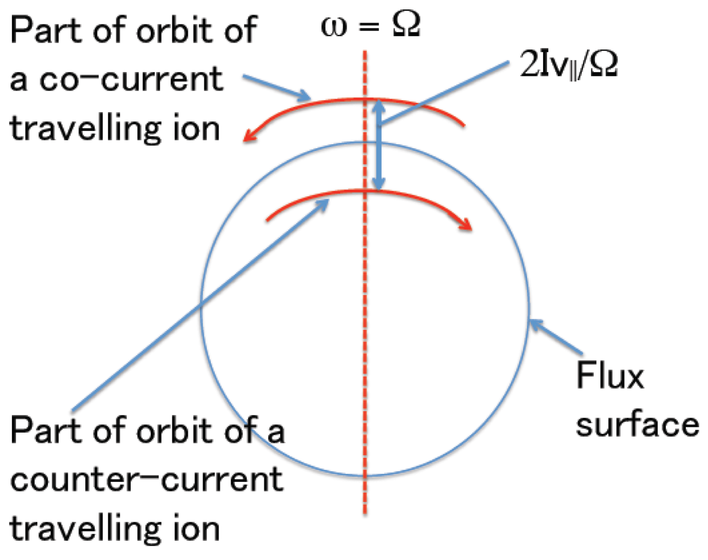
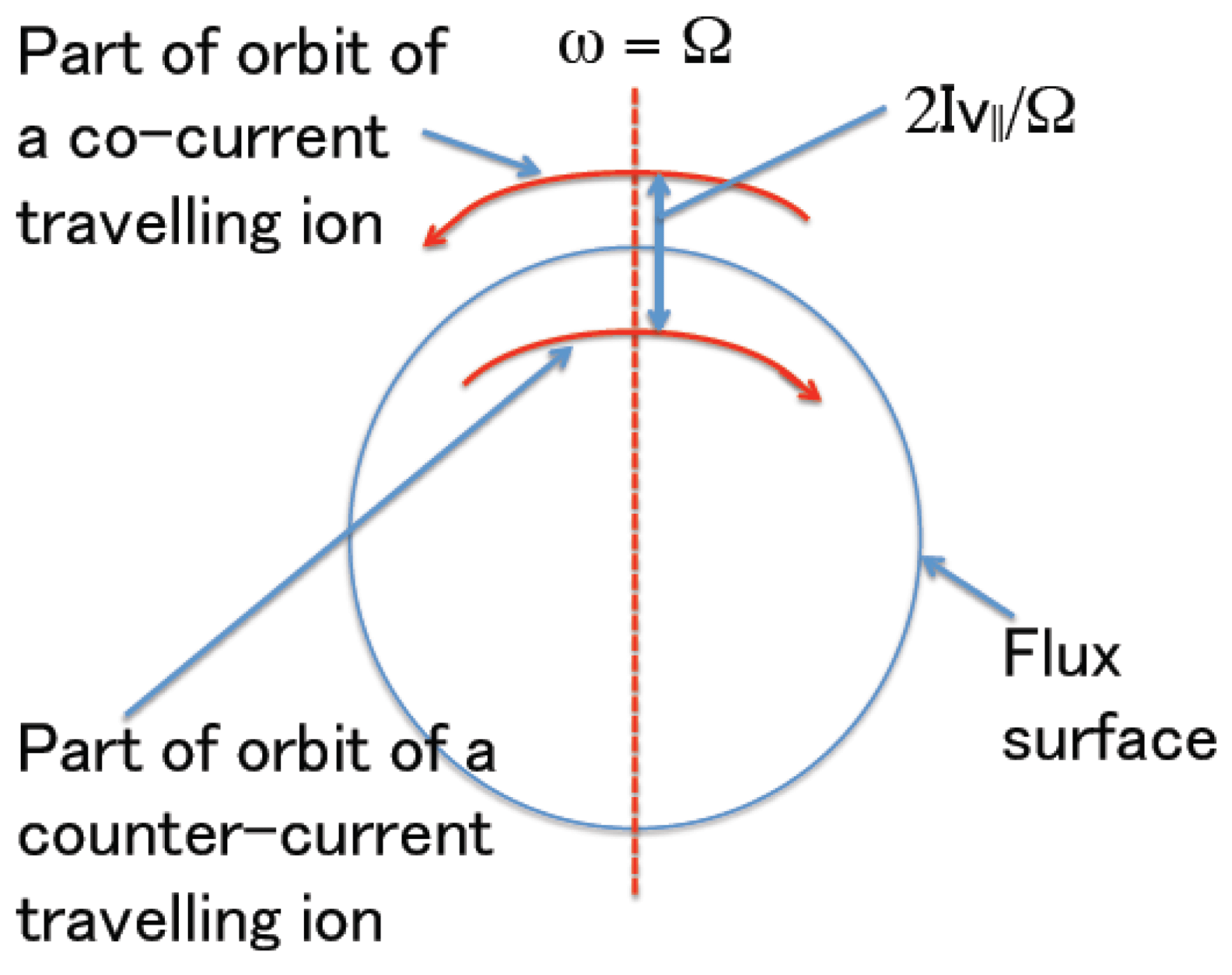
charges are heated more than the co-current directed ones. As shown in figure 1, the heating difference between the counter and co-moving ions occurs because the counter (co) have a longer (shorter) interaction time with the applied radio frequency (rf) as discussed in §§ 4 and 5. As an example, the current driven by a symmetric spectrum is evaluated for a near Maxwellian minority species in § 5. In this limit the driven current is found to be rather modest so is unlikely to be useful. However, minority heating levels are often large enough to result in substantial departures from a Maxwellian. Therefore, it may be possible to drive significant minority counter-current with a symmetric spectrum, and thereby generate beneficial driven co-current. Detailed simulations seem necessary to make this determination. These could even be performed for deuterium and energetic alpha minorities in a tritium plasma.
More (less) minority heating always occurs in the counter (co) current direction because the interaction time
 $\unicode[STIX]{x1D70F}_{\text{int}}\propto q/\unicode[STIX]{x1D700}$
for the counter (co) travelling minorities that are closer to (further from) the magnetic axis is longer (shorter) as shown here schematically. Therefore, excess minority heating always occurs in the favourable counter-current direction.
Once we evaluate the parallel flow of the energetic minorities,
 $V_{||m}$
, for a symmetric spectrum it is important to ascertain the direction of the overall parallel current that is driven to determine if it is in the desirable co-current direction or the unfavourable counter-current direction. To make this determination we follow the insights outlined by Fisch (Reference Fisch1981) for a conventional minority current drive that relies on an asymmetry in the collisional heating. When there is no net parallel momentum input we assume we must satisfy
 $$\begin{eqnarray}\displaystyle Mn_{m}V_{||m}+mn_{e}V_{||e}+M_{i}n_{i}V_{||i}=0 & & \displaystyle\end{eqnarray}$$
in our quasineutral plasma with
 $$\begin{eqnarray}\displaystyle Zn_{m}+Z_{i}n_{i}=n_{e}. & & \displaystyle\end{eqnarray}$$
We use
 $n$
,
 $V_{||}$
,
 $Z$
and
 $M$
to signify density, parallel fluid velocity, charge number and mass, with the subscripts
 $i$
,
 $e$
and
 $m$
denoting background ion, electron and minority species, with
 $m$
the electron mass and
 $Z=-1$
the electron charge. The
 $m$
subscript is suppressed on the minority charge number
 $Z$
and mass
 $M$
. The friction between the electrons, and minorities and background ions must vanish (Fisch Reference Fisch1981) to lowest order to satisfy the parallel electron momentum equation giving
 $$\begin{eqnarray}\displaystyle Z^{2}n_{m}(V_{||m}-V_{||e})+Z_{i}^{2}n_{i}(V_{||i}-V_{||e})=0. & & \displaystyle\end{eqnarray}$$
This friction equation is more carefully obtained by multiplying the parallel electron momentum equation by the magnetic field
 $B$
and then flux surface averaging to annihilate the electron pressure and the electrostatic potential term (assuming Maxwell–Boltzmann responses to lowest order). As we are not concerned about inverse aspect ratio corrections, the procedure of Fisch (Reference Fisch1981) is adequate for our purposes.
These three equations determine the direction of the parallel current
 $$\begin{eqnarray}\displaystyle J_{||}=Zen_{m}V_{||m}+Z_{i}en_{i}V_{||i}-n_{e}eV_{||e} & & \displaystyle\end{eqnarray}$$
once the direction of
 $V_{||m}$
is known, as can be seen by neglecting the parallel momentum of the electrons as small to find
 $$\begin{eqnarray}\displaystyle M_{i}n_{i}V_{||i}=-Mn_{m}V_{||m}, & & \displaystyle\end{eqnarray}$$
and then using the vanishing of the electron friction to obtain
 $$\begin{eqnarray}\displaystyle V_{||e}=\frac{Z^{2}n_{m}V_{||m}+n_{i}V_{||i}}{Z^{2}n_{m}+Z_{i}^{2}n_{i}}=\frac{(Z^{2}-Z_{i}^{2}M/M_{i})n_{m}V_{||m}}{Z^{2}n_{m}+Z_{i}^{2}n_{i}}. & & \displaystyle\end{eqnarray}$$
From these expressions we can already see that a negative parallel minority flow
 $(V_{||m}<0)$
, results in a positive parallel main ion flow
 $(V_{||i}>0)$
and a negative parallel electron flow
 $(V_{||e}<0)$
, thereby resulting in the possibility of co-current being driven. Eliminating
 $V_{||e}$
and
 $V_{||i}$
the symmetric spectrum co-current can be written as
 $$\begin{eqnarray}\displaystyle J_{||}=-Zen_{m}V_{||m}\frac{Z_{i}(Z-Z_{i})(n_{i}-Mn_{m}/M_{i})}{Z_{i}^{2}n_{i}+Z^{2}n_{m}}, & & \displaystyle\end{eqnarray}$$
which for
 $V_{||m}<0$
and
 $Z>Z_{i}$
will be co-current as long as
 $n_{i}>Mn_{m}/M_{i}$
. In the subsequent sections we will demonstrate that when finite poloidal gyroradius effects are retained, a counter-current minority flow is ordinarily driven. Therefore, when a minority species is present a symmetric heating spectrum will normally result in co-current drive.
We also consider a second example of minority deuterium (D) heating in a tritium (T) plasma in § 6. In this case the amount of alpha counter-current driven tends to remain small as the alpha density is much smaller than the plasma density. However, at high minority heating levels it may be possible to drive modest and perhaps even significant co-current. The closing section summarizes results, but also discusses other possible ways to drive co-current with a symmetric spectrum.
2 Formulation of the quasilinear equation
We start with full Fokker–Planck kinetic equation
 $$\begin{eqnarray}\displaystyle \unicode[STIX]{x2202}f/\unicode[STIX]{x2202}t+\boldsymbol{v}\boldsymbol{\cdot }\unicode[STIX]{x1D735}f+(Ze/M)[\boldsymbol{e}+c^{-1}\boldsymbol{v}\times (\boldsymbol{B}+\boldsymbol{b})]\boldsymbol{\cdot }\unicode[STIX]{x1D735}_{v}f=C\{\,f\}, & & \displaystyle\end{eqnarray}$$
with
 $\boldsymbol{e}=\boldsymbol{e}(\boldsymbol{r},t)$
and
 $\boldsymbol{b}=\boldsymbol{b}(\boldsymbol{r},t)$
the applied radio frequency (rf) wave fields satisfying Faraday’s law, and
 $\boldsymbol{B}$
the unperturbed, axisymmetric magnetic field
 $$\begin{eqnarray}\displaystyle \boldsymbol{B}=B\boldsymbol{n}=I(\unicode[STIX]{x1D713})\unicode[STIX]{x1D735}\unicode[STIX]{x1D701}+\unicode[STIX]{x1D735}\unicode[STIX]{x1D701}\times \unicode[STIX]{x1D735}\unicode[STIX]{x1D713}. & & \displaystyle\end{eqnarray}$$
Here
 $\unicode[STIX]{x1D701}$
is the toroidal angle variable and
 $I=RB_{t}$
is a function of the poloidal flux function
 $\unicode[STIX]{x1D713}$
, with
 $B_{t}$
and
 $B_{p}$
the toroidal and poloidal magnetic fields. We denote
 $\boldsymbol{e}_{1}$
as the unit vector in the
 $\unicode[STIX]{x1D735}\unicode[STIX]{x1D713}$
direction by taking
 $\unicode[STIX]{x1D735}\unicode[STIX]{x1D713}=RB_{p}\boldsymbol{e}_{1}$
, and let
 $\boldsymbol{e}_{2}=\boldsymbol{n}\times \boldsymbol{e}_{1}$
be the orthonormal unit vector. The notation is as in Catto et al. (Reference Catto, Lee and Ram2017).
Our quasilinear treatment begins in what appears to be the usual manner by taking
 $$\begin{eqnarray}\displaystyle f=f_{0}+f_{1}+\cdots \,, & & \displaystyle\end{eqnarray}$$
with
 $f_{1}\ll \,f_{0}$
. However, the unperturbed drift kinetic operator acting on the unperturbed distribution function
 $f_{0}$
must vanish for the gyrophase independent drift kinetic canonical angular momentum, as recalled in (2.8) below. The full gyrophase dependent canonical angular momentum
 $\unicode[STIX]{x1D713}_{\ast }$
is
 $$\begin{eqnarray}\displaystyle \unicode[STIX]{x1D713}_{\ast }\equiv \unicode[STIX]{x1D713}-(Mc/Ze)R^{2}\unicode[STIX]{x1D735}\unicode[STIX]{x1D701}\boldsymbol{\cdot }\boldsymbol{v}\equiv \bar{\unicode[STIX]{x1D713}}_{\ast }+\unicode[STIX]{x1D6FA}^{-1}\boldsymbol{v}\times \boldsymbol{n}\boldsymbol{\cdot }\unicode[STIX]{x1D735}\unicode[STIX]{x1D713}, & & \displaystyle\end{eqnarray}$$
where the drift kinetic form
 $\bar{\unicode[STIX]{x1D713}}_{\ast }$
written in terms of
 $\unicode[STIX]{x1D713},\unicode[STIX]{x1D717},v,\unicode[STIX]{x1D707}$
, and
 $\unicode[STIX]{x1D70E}$
is
 $$\begin{eqnarray}\displaystyle \bar{\unicode[STIX]{x1D713}}_{\ast }\equiv \unicode[STIX]{x1D713}-Iv_{||}/\unicode[STIX]{x1D6FA}=\unicode[STIX]{x1D713}-\unicode[STIX]{x1D6FA}^{-1}I\unicode[STIX]{x1D70E}\sqrt{v^{2}-2\unicode[STIX]{x1D707}_{0}B}=\unicode[STIX]{x1D713}-\unicode[STIX]{x1D6FA}^{-1}Iv\unicode[STIX]{x1D70E}\sqrt{1-\unicode[STIX]{x1D706}B/B_{0}}, & & \displaystyle\end{eqnarray}$$
with
 $\unicode[STIX]{x1D6FA}=ZeB/Mc$
,
 $\unicode[STIX]{x1D707}_{0}=v_{\bot }^{2}/2B(\boldsymbol{r})$
the lowest order magnetic moment,
 $\unicode[STIX]{x1D70E}=v_{||}/|v_{||}|$
the sign of
 $v_{||}=\boldsymbol{n}\boldsymbol{\cdot }\boldsymbol{v}=\unicode[STIX]{x1D70E}\sqrt{v^{2}-2\unicode[STIX]{x1D707}_{0}B}$
,
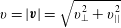
 $v$
the speed
 $v=|\boldsymbol{v}|=\sqrt{v_{\bot }^{2}+v_{||}^{2}}$
,
 $\unicode[STIX]{x1D706}=2\unicode[STIX]{x1D707}_{0}B_{0}/v^{2}$
,
 $\unicode[STIX]{x1D717}$
the poloidal angle,
 $\unicode[STIX]{x1D711}$
the gyrophase, and
 $$\begin{eqnarray}\displaystyle \boldsymbol{v}=\boldsymbol{v}_{\bot }+v_{||}\boldsymbol{n}=v_{\bot }[\boldsymbol{e}_{1}(\boldsymbol{r})\cos \unicode[STIX]{x1D711}+\boldsymbol{e}_{2}(\boldsymbol{r})\sin \unicode[STIX]{x1D711}]+v_{||}\boldsymbol{n}(\boldsymbol{r}). & & \displaystyle\end{eqnarray}$$
The normalizing magnetic field is
 $B_{0}=\sqrt{\langle B^{2}\rangle }$
with
 $\langle \cdots \rangle$
a flux surface average. The last term in (2.4) is the difference between the guiding centre and particle locations, while the
 $Iv_{||}/\unicode[STIX]{x1D6FA}$
term in (2.5) keeps the distinction between the flux and drift surfaces.
A drift kinetic treatment for
 $f_{0}$
can depend on the drift kinetic constant of the motion
 $\bar{\unicode[STIX]{x1D713}}_{\ast }$
that we treat as a dependent variable. Hence, we allow
 $$\begin{eqnarray}\displaystyle f_{0}=f_{0}(\bar{\unicode[STIX]{x1D713}}_{\ast };\unicode[STIX]{x1D713},\unicode[STIX]{x1D717},v,\unicode[STIX]{x1D707},\unicode[STIX]{x1D70E},t), & & \displaystyle\end{eqnarray}$$
with
 $\unicode[STIX]{x1D713},\unicode[STIX]{x1D717},v,\unicode[STIX]{x1D707},\unicode[STIX]{x1D70E}$
and
 $t$
the same independent drift kinetic variables as in Catto et al. (Reference Catto, Lee and Ram2017), most of whose results we will be able to adopt.
The notation in (2.7) is intended to indicate that
 $\bar{\unicode[STIX]{x1D713}}_{\ast }$
is a dependent variable and
 $\unicode[STIX]{x1D713}$
is an independent variable, thereby allowing us to distinguish between finite orbit effects and flux surface variation. The notation will allow us to explicitly display the velocity dependent finite departure of a drift surface from a flux surface.
The drift kinetic canonical angular momentum
 $\bar{\unicode[STIX]{x1D713}}_{\ast }$
is convenient to employ because it is a drift kinetic constant of the motion satisfying
 $$\begin{eqnarray}\displaystyle (v_{||}\boldsymbol{n}+\boldsymbol{v}_{d})\boldsymbol{\cdot }\unicode[STIX]{x1D735}\bar{\unicode[STIX]{x1D713}}_{\ast }=-\boldsymbol{v}_{d}\boldsymbol{\cdot }\unicode[STIX]{x1D735}(Iv_{||}/\unicode[STIX]{x1D6FA})=0, & & \displaystyle\end{eqnarray}$$
(as shown in appendix B of Parra & Catto (Reference Parra and Catto2010)) where we also use
 $\boldsymbol{v}_{d}\boldsymbol{\cdot }\unicode[STIX]{x1D735}\unicode[STIX]{x1D713}=v_{||}\boldsymbol{n}\boldsymbol{\cdot }\unicode[STIX]{x1D735}(Iv_{||}/\unicode[STIX]{x1D6FA})$
. Here we denote
 $\boldsymbol{v}_{d}$
as the magnetic drift,
 $$\begin{eqnarray}\displaystyle \boldsymbol{v}_{d}=\unicode[STIX]{x1D6FA}^{-1}\boldsymbol{n}\times (\unicode[STIX]{x1D707}\unicode[STIX]{x1D735}B+v_{||}^{2}\boldsymbol{n}\boldsymbol{\cdot }\unicode[STIX]{x1D735}\boldsymbol{n})=\unicode[STIX]{x1D6FA}^{-1}v_{||}\unicode[STIX]{x1D735}\times (v_{||}\boldsymbol{n}). & & \displaystyle\end{eqnarray}$$
By using total energy
 $E=v^{2}/2+Ze\unicode[STIX]{x1D6F7}(\unicode[STIX]{x1D713})/M$
instead of
 $v$
, as we could generalize to retain the
 $\boldsymbol{E}\times \boldsymbol{B}$
drift as well. To retain drift effects in the quasilinear operator we must allow
 $f_{0}$
to depend on the magnetic moment to higher order as shown by Catto et al. (Reference Catto, Lee and Ram2017). Therefore, we use
 $\unicode[STIX]{x1D707}=\unicode[STIX]{x1D707}_{0}+\unicode[STIX]{x1D707}_{1}$
, where Catto et al. (Reference Catto, Lee and Ram2017) prove that only
 $\unicode[STIX]{x1D707}_{1}\rightarrow -B^{-1}\boldsymbol{v}_{\bot }\boldsymbol{\cdot }\boldsymbol{v}_{d}$
and
 $B\unicode[STIX]{x1D735}_{v}\unicode[STIX]{x1D707}\rightarrow \boldsymbol{v}_{\bot }-\boldsymbol{v}_{d}$
need be retained.
When parallel streaming and finite orbit effects compete and dominate the lowest order drift kinetic equation is
 $$\begin{eqnarray}\displaystyle (v_{||}\boldsymbol{n}+\boldsymbol{v}_{d})\boldsymbol{\cdot }\unicode[STIX]{x1D735}\bar{f}_{0}=0, & & \displaystyle\end{eqnarray}$$
with
 $f_{0}=\bar{f}_{0}+\tilde{f}_{0}$
,
 $\bar{f}_{0}\gg \tilde{f}_{0}$
, and
 $$\begin{eqnarray}\displaystyle \bar{f}_{0}=\bar{f}_{0}(\bar{\unicode[STIX]{x1D713}}_{\ast },v,\unicode[STIX]{x1D707},\unicode[STIX]{x1D70E}), & & \displaystyle\end{eqnarray}$$
indicating that the
 $\unicode[STIX]{x1D713}$
and
 $\unicode[STIX]{x1D717}$
dependence can only enter through
 $\bar{\unicode[STIX]{x1D713}}_{\ast }$
.
When streaming does not dominate, the introduction of
 $\bar{\unicode[STIX]{x1D713}}_{\ast }$
is of no benefit. Then
 $f_{0}$
satisfies the quasilinear (QL) equation
 $$\begin{eqnarray}\displaystyle \unicode[STIX]{x2202}f_{0}/\unicode[STIX]{x2202}t+(v_{||}\boldsymbol{n}+\boldsymbol{v}_{d})\boldsymbol{\cdot }\unicode[STIX]{x1D735}f_{0}+\langle \boldsymbol{a}\boldsymbol{\cdot }\unicode[STIX]{x1D735}_{v}f_{1}\rangle _{cg,\unicode[STIX]{x1D711}}=\langle C\{f_{0}\}\rangle _{\unicode[STIX]{x1D711}}, & & \displaystyle\end{eqnarray}$$
with the perturbed acceleration defined as
 $$\begin{eqnarray}\displaystyle \boldsymbol{a}=(Ze/M)(\boldsymbol{e}+c^{-1}\boldsymbol{v}\times \boldsymbol{b}), & & \displaystyle\end{eqnarray}$$
and the gyroaverages
 $\langle \cdots \rangle _{\unicode[STIX]{x1D711}}$
performed at fixed
 $\unicode[STIX]{x1D713},\unicode[STIX]{x1D717},v,\unicode[STIX]{x1D707},\unicode[STIX]{x1D70E}$
, and
 $t$
,
 $$\begin{eqnarray}\displaystyle \langle \cdots \rangle _{\unicode[STIX]{x1D711}}=(2\unicode[STIX]{x03C0})^{-1}\oint \text{d}\unicode[STIX]{x1D711}(\cdots ). & & \displaystyle\end{eqnarray}$$
Quasilinear theory assumes that
 $f_{0}$
does not contain any fast time or space variation and that collisions and quasilinear diffusion compete. As a result, we take
 $f_{0}$
to be the coarse grain average of
 $f$
,
 $$\begin{eqnarray}\displaystyle f_{0}=\langle f\rangle _{cg}=\frac{1}{2T}\int _{t-T}^{t+T}\text{d}\unicode[STIX]{x1D70F}\frac{1}{2\unicode[STIX]{x1D6E5}}\int _{\unicode[STIX]{x1D713}-\unicode[STIX]{x1D6E5}}^{\unicode[STIX]{x1D713}+\unicode[STIX]{x1D6E5}}\text{d}\unicode[STIX]{x1D713}^{\prime }\oint \frac{\text{d}\unicode[STIX]{x1D701}}{2\unicode[STIX]{x03C0}}\langle f\rangle _{\unicode[STIX]{x1D717}}, & & \displaystyle\end{eqnarray}$$
where the integral over toroidal angle
 $\unicode[STIX]{x1D701}$
insures axisymmetry, and the average
 $\langle \cdots \rangle _{\unicode[STIX]{x1D717}}$
over poloidal angle
 $\unicode[STIX]{x1D717}$
removes the exponential poloidal mode number variation. We must allow
 $Q\{f_{0}\}$
to be a slow function of
 $\unicode[STIX]{x1D717}$
in a tokamak so
 $\langle \cdots \rangle _{\unicode[STIX]{x1D717}}\neq (2\unicode[STIX]{x03C0})^{-1}\oint \text{d}\unicode[STIX]{x1D717}(\cdots )$
. The integral over
 $\unicode[STIX]{x1D70F}$
removes fast time variation by taking
 $\unicode[STIX]{x1D714}^{-1}\ll T\ll \unicode[STIX]{x1D708}^{-1}$
, where
 $\unicode[STIX]{x1D708}$
and
 $\unicode[STIX]{x1D714}$
are the collision frequency and typical rf wave frequency, respectively. The limits on the poloidal flux function
 $\unicode[STIX]{x1D713}$
integral resolve poloidal gyroradius scales by assuming
 $\unicode[STIX]{x1D6E5}\ll \unicode[STIX]{x1D70C}_{p}$
, where
 $\unicode[STIX]{x1D70C}_{p}=\unicode[STIX]{x1D70C}B/B_{p}$
is the poloidal gyroradius, with
 $\unicode[STIX]{x1D70C}$
the species gyroradius. The radial and
 $\langle \cdots \rangle _{\unicode[STIX]{x1D717}}$
averages are defined so that the entropy production is negative definite, with
 $f_{0}$
allowed to be a slow function of
 $\unicode[STIX]{x1D713}$
and
 $\unicode[STIX]{x1D717}$
.
We define the quasilinear operator
 $Q$
by
 $$\begin{eqnarray}\displaystyle Q\{f_{0}\}=-\langle \unicode[STIX]{x1D735}_{v}\boldsymbol{\cdot }(\boldsymbol{a}f_{1})\rangle _{cg,\unicode[STIX]{x1D711}}=-\unicode[STIX]{x1D735}_{v}\boldsymbol{\cdot }\langle \boldsymbol{a}f_{1}\rangle _{cg,\unicode[STIX]{x1D711}}, & & \displaystyle\end{eqnarray}$$
where the drift kinetic treatment in
 $\unicode[STIX]{x1D713},\unicode[STIX]{x1D717},v,\unicode[STIX]{x1D707},\unicode[STIX]{x1D70E}$
, and
 $t$
variables requires that we average the QL term over gyrophase, as well as perform a coarse grain average. The drift kinetic equation then becomes
 $$\begin{eqnarray}\displaystyle \unicode[STIX]{x2202}f_{0}/\unicode[STIX]{x2202}t+(v_{||}\boldsymbol{n}+\boldsymbol{v}_{d})\boldsymbol{\cdot }\unicode[STIX]{x1D735}f_{0}=C\{f_{0}\}+Q\{f_{0}\}. & & \displaystyle\end{eqnarray}$$
Rotational invariance allows us to use
 $\langle C\{f_{0}\}\rangle _{\unicode[STIX]{x1D711}}=C\{f_{0}\}$
as there is no preferred direction associated with the collision operator.
The preceding equation implicitly allows us to retain
 $\bar{\unicode[STIX]{x1D713}}_{\ast }$
as a dependent variable when the streaming combination of (2.10) dominates due to finite orbit effects such that to lowest order
 $f_{0}\rightarrow \bar{f}_{0}(\bar{\unicode[STIX]{x1D713}}_{\ast },v,\unicode[STIX]{x1D707},\unicode[STIX]{x1D70E})$
. Equation (2.17) is the same as Catto et al. (Reference Catto, Lee and Ram2017) since it only differs by the introduction of a dependent variable
 $\bar{\unicode[STIX]{x1D713}}_{\ast }$
to track finite orbit affects. That is, we now write
 $f_{0}=f_{0}(\bar{\unicode[STIX]{x1D713}}_{\ast };\unicode[STIX]{x1D713},\unicode[STIX]{x1D717},v,\unicode[STIX]{x1D707},\unicode[STIX]{x1D70E},t)$
, rather than using
 $f_{0}=f_{0}(\unicode[STIX]{x1D713},\unicode[STIX]{x1D717},v,\unicode[STIX]{x1D707},\unicode[STIX]{x1D70E},t)$
– a form that does not allow us to explicitly display
 $\bar{\unicode[STIX]{x1D713}}_{\ast }$
or ‘radial’ spatial derivatives of
 $f_{0}$
when the velocity space gradient is performed.
Here we also emphasize that our result for the quasilinear operator must have the property that it does not act as a source or sink of particles since
 $$\begin{eqnarray}\displaystyle \int \text{d}^{3}vQ\{f_{0}\}=-\int \text{d}^{3}v\unicode[STIX]{x1D735}_{v}\boldsymbol{\cdot }\langle \boldsymbol{a}f_{1}\rangle _{cg}=0. & & \displaystyle\end{eqnarray}$$
That is, in drift kinetic variables, there can be no diffusive spatial particle transport (or source or sink of particles) due to the operator
 $Q\{f_{0}\}$
. Such a statement might appear to contradict the results of Kaufman (Reference Kaufman1972) and Eriksson & Helander (Reference Eriksson and Helander1994), but their treatments are in canonical variables that mix configuration and velocity space and thereby only appear to introduce a radial spatial derivative as we will demonstrate in § 3.
We allow both spatial heat and parallel momentum diffusive transport since
 $$\begin{eqnarray}\displaystyle \int \text{d}^{3}vv^{2}Q\{f_{0}\}=2(Ze/M)\left\langle \boldsymbol{e}\boldsymbol{\cdot }\int \text{d}^{3}v\boldsymbol{v}f_{1}\right\rangle _{cg}\neq 0 & & \displaystyle\end{eqnarray}$$
and
 $$\begin{eqnarray}\displaystyle \int \text{d}^{3}v\boldsymbol{v}Q\{\,f_{0}\}=\int \text{d}^{3}v\langle \boldsymbol{a}f_{1}\rangle _{cg}\neq 0. & & \displaystyle\end{eqnarray}$$
Our choice of independent variables means we can simply adopt the quasilinear operator obtained by Catto et al. (Reference Catto, Lee and Ram2017) to illustrate how finite orbit effects enter.
3 Quasilinear operator
Catto et al. (Reference Catto, Lee and Ram2017) derive the following self-adjoint form for the QL operator:
 $$\begin{eqnarray}\displaystyle Q\{f_{0}\}=\mathop{\sum }_{\unicode[STIX]{x1D714},p}\frac{v_{||}}{v}\left(\frac{\unicode[STIX]{x2202}}{\unicode[STIX]{x2202}v}+\frac{p\unicode[STIX]{x1D6FA}v}{\unicode[STIX]{x1D714}B}\frac{\unicode[STIX]{x2202}}{\unicode[STIX]{x2202}\unicode[STIX]{x1D707}_{0}}\right)\left[D\frac{v}{v_{||}}\left(\frac{\unicode[STIX]{x2202}f_{0}}{\unicode[STIX]{x2202}v}+\frac{p\unicode[STIX]{x1D6FA}v}{\unicode[STIX]{x1D714}B}\frac{\unicode[STIX]{x2202}f_{0}}{\unicode[STIX]{x2202}\unicode[STIX]{x1D707}_{0}}\right)\right], & & \displaystyle\end{eqnarray}$$
with
 $p\unicode[STIX]{x1D6FA}=\unicode[STIX]{x1D714}-k_{||}v_{||}-\boldsymbol{k}\boldsymbol{\cdot }\boldsymbol{v}_{d}$
, and
 $$\begin{eqnarray}\displaystyle D=\frac{\unicode[STIX]{x03C0}Z^{2}e^{2}}{2M^{2}v^{2}}\mathop{\sum }_{\unicode[STIX]{x1D705},m,n}\unicode[STIX]{x1D6FF}(\unicode[STIX]{x1D714}-p\unicode[STIX]{x1D6FA}-k_{||}v_{||}-\boldsymbol{k}\boldsymbol{\cdot }\boldsymbol{v}_{d})|\boldsymbol{e}_{m}\boldsymbol{\cdot }[\boldsymbol{n}v_{||}J_{p}(w)+\boldsymbol{e}_{\bot p}v_{\bot }]|^{2}, & & \displaystyle\end{eqnarray}$$
manifestly positive, with no quasilinear particle diffusion as required by (2.18). In this final form the entropy production is negative definite, and it is no longer necessary to keep the distinction between
 $\unicode[STIX]{x1D707}$
and
 $\unicode[STIX]{x1D707}_{0}$
, so we may now use
 $d^{3}v\rightarrow 2\unicode[STIX]{x03C0}vB\,\text{d}v\,\text{d}\unicode[STIX]{x1D707}_{0}/v_{||}$
. To obtain this form the applied fluctuating electric field
 $\boldsymbol{e}=\boldsymbol{e}(\boldsymbol{r},t)$
is Fourier decomposed poloidally (
 $m$
) and toroidally (
 $n$
), permitted to have more than a single applied wave frequency by Fourier decomposing in time, and allowed to possess local fine scale radial eikonal variation with multiple roots (sum over
 $\unicode[STIX]{x1D705}$
) due to mode conversion. Therefore, we take
 $$\begin{eqnarray}\displaystyle \boldsymbol{e}=\boldsymbol{e}(\boldsymbol{r},t)=\mathop{\sum }_{m,n,\unicode[STIX]{x1D714},\unicode[STIX]{x1D705}}\boldsymbol{e}_{m}\text{e}^{-\text{i}\unicode[STIX]{x1D714}t-\text{i}n\unicode[STIX]{x1D701}+\text{i}S(\unicode[STIX]{x1D713})+\text{i}m\unicode[STIX]{x1D717}}, & & \displaystyle\end{eqnarray}$$
with
 $w\equiv k_{\bot }v_{\bot }/\unicode[STIX]{x1D6FA}$
the argument of the Bessel functions,
 $$\begin{eqnarray}\displaystyle & \displaystyle \unicode[STIX]{x1D73F}=\unicode[STIX]{x1D735}S=\unicode[STIX]{x1D735}\unicode[STIX]{x1D713}\unicode[STIX]{x2202}S/\unicode[STIX]{x2202}\unicode[STIX]{x1D713}=\boldsymbol{e}_{1}RB_{p}\unicode[STIX]{x2202}S/\unicode[STIX]{x2202}\unicode[STIX]{x1D713}=\unicode[STIX]{x1D705}\boldsymbol{e}_{1}, & \displaystyle\end{eqnarray}$$
 $$\begin{eqnarray}\displaystyle & \displaystyle k_{||}=(m-qn)I/qR^{2}B\sim (m-qn)/qR, & \displaystyle\end{eqnarray}$$
 $$\begin{eqnarray}\displaystyle & \displaystyle \boldsymbol{k}=\unicode[STIX]{x1D73F}+m\unicode[STIX]{x1D735}\unicode[STIX]{x1D717}-n\unicode[STIX]{x1D735}\unicode[STIX]{x1D701}, & \displaystyle\end{eqnarray}$$
 $$\begin{eqnarray}\displaystyle & \displaystyle \boldsymbol{e}_{\bot p}=\frac{1}{2}[\boldsymbol{e}_{-}\text{e}^{\text{i}\unicode[STIX]{x1D6FC}}J_{p+1}(w)+\boldsymbol{e}_{+}\text{e}^{-\text{i}\unicode[STIX]{x1D6FC}}J_{p-1}(w)]=\frac{p}{k_{\bot }w}J_{p}(w)\boldsymbol{k}_{\bot }+\frac{\text{i}}{k_{\bot }}J_{p}^{\prime }(w)\boldsymbol{n}\times \boldsymbol{k}, & \displaystyle\end{eqnarray}$$
 $$\begin{eqnarray}\displaystyle & \displaystyle \boldsymbol{k}_{\bot }=(k_{\bot }/2)(\boldsymbol{e}_{-}\text{e}^{\text{i}\unicode[STIX]{x1D6FC}}+\boldsymbol{e}_{+}\text{e}^{-\text{i}\unicode[STIX]{x1D6FC}}), & \displaystyle\end{eqnarray}$$
and
 $$\begin{eqnarray}\displaystyle \boldsymbol{e}_{\pm }=\boldsymbol{e}_{1}\pm \text{i}\boldsymbol{e}_{2}, & & \displaystyle\end{eqnarray}$$
where
 $\boldsymbol{e}_{+}$
is the left-hand polarized wave direction of minority heating and current drive. Preserving the desired entropy production property requires
 $$\begin{eqnarray}\displaystyle \langle \boldsymbol{e}\boldsymbol{e}\rangle _{cg}=\frac{1}{4}\mathop{\sum }_{\unicode[STIX]{x1D714},m,n\cdot \unicode[STIX]{x1D705}}(\boldsymbol{e}_{m}\boldsymbol{e}_{m}^{\ast }\,+\,\boldsymbol{e}_{m}^{\ast }\boldsymbol{e}_{m}). & & \displaystyle\end{eqnarray}$$
Equations (3.1) and (3.2) are the results of Catto et al. (Reference Catto, Lee and Ram2017). They reduce to the QL operator of Kennel & Engelmann (Reference Kennel and Engelmann1966) in a constant magnetic field. Our QL ordering like theirs allows
 $Q\sim C$
or
 $D/v_{\text{tail}}^{2}\sim \unicode[STIX]{x1D708}$
, with
 $D\sim Z^{2}e^{2}|\boldsymbol{e}_{m}|^{2}/M^{2}\unicode[STIX]{x1D714}\sim \unicode[STIX]{x1D714}v_{\text{quiv}}^{2}$
and
 $v_{\text{quiv}}\sim Ze|\boldsymbol{e}_{m}|/M\unicode[STIX]{x1D714}$
. It requires small quiver speeds
 $v_{\text{quiv}}$
compared to the typical minority ion tail speed
 $v_{\text{tail}}$
to satisfy
 $v_{\text{quiv}}^{2}/v_{\text{tail}}^{2}\sim \unicode[STIX]{x1D708}/\unicode[STIX]{x1D714}\ll 1$
.
To display finite orbit effects we can employ the dependent variable
 $\bar{\unicode[STIX]{x1D713}}_{\ast }$
to write
 $$\begin{eqnarray}\displaystyle \frac{\unicode[STIX]{x2202}}{\unicode[STIX]{x2202}v}=\left.\frac{\unicode[STIX]{x2202}}{\unicode[STIX]{x2202}v}\right|_{\bar{\unicode[STIX]{x1D713}}_{\ast }}+\left.\frac{\unicode[STIX]{x2202}\bar{\unicode[STIX]{x1D713}}_{\ast }}{\unicode[STIX]{x2202}v}\right|_{\unicode[STIX]{x1D707}_{0}}\frac{\unicode[STIX]{x2202}}{\unicode[STIX]{x2202}\bar{\unicode[STIX]{x1D713}}_{\ast }}=\left.\frac{\unicode[STIX]{x2202}}{\unicode[STIX]{x2202}v}\right|_{\bar{\unicode[STIX]{x1D713}}_{\ast }}-\frac{Iv}{\unicode[STIX]{x1D6FA}v_{||}}\frac{\unicode[STIX]{x2202}}{\unicode[STIX]{x2202}\bar{\unicode[STIX]{x1D713}}_{\ast }} & & \displaystyle\end{eqnarray}$$
and
 $$\begin{eqnarray}\displaystyle \frac{\unicode[STIX]{x2202}}{\unicode[STIX]{x2202}\unicode[STIX]{x1D707}_{0}}=\left.\frac{\unicode[STIX]{x2202}}{\unicode[STIX]{x2202}\unicode[STIX]{x1D707}_{0}}\right|_{\bar{\unicode[STIX]{x1D713}}_{\ast }}+\left.\frac{\unicode[STIX]{x2202}\bar{\unicode[STIX]{x1D713}}_{\ast }}{\unicode[STIX]{x2202}\unicode[STIX]{x1D707}_{0}}\right|_{v}\frac{\unicode[STIX]{x2202}}{\unicode[STIX]{x2202}\bar{\unicode[STIX]{x1D713}}_{\ast }}=\left.\frac{\unicode[STIX]{x2202}}{\unicode[STIX]{x2202}\unicode[STIX]{x1D707}_{0}}\right|_{\bar{\unicode[STIX]{x1D713}}_{\ast }}+\frac{IB}{\unicode[STIX]{x1D6FA}v_{||}}\frac{\unicode[STIX]{x2202}}{\unicode[STIX]{x2202}\bar{\unicode[STIX]{x1D713}}_{\ast }}. & & \displaystyle\end{eqnarray}$$
In this notation (3.1) gives an alternate, but not particularly useful, form displaying the effect of finite orbits by the appearance of derivatives with respect to
 $\bar{\unicode[STIX]{x1D713}}_{\ast }$
:
 $$\begin{eqnarray}\displaystyle Q\{\,f_{0}\} & = & \displaystyle \mathop{\sum }_{\unicode[STIX]{x1D714},p}\frac{v_{||}}{v}\left[\left.\frac{\unicode[STIX]{x2202}}{\unicode[STIX]{x2202}v}\right|_{\bar{\unicode[STIX]{x1D713}}_{\ast }}+\frac{p\unicode[STIX]{x1D6FA}v}{\unicode[STIX]{x1D714}B}\left.\frac{\unicode[STIX]{x2202}}{\unicode[STIX]{x2202}\unicode[STIX]{x1D707}_{0}}\right|_{\bar{\unicode[STIX]{x1D713}}_{\ast }}-\left(1-\frac{p\unicode[STIX]{x1D6FA}}{\unicode[STIX]{x1D714}}\right)\frac{Iv}{\unicode[STIX]{x1D6FA}v_{||}}\frac{\unicode[STIX]{x2202}}{\unicode[STIX]{x2202}\bar{\unicode[STIX]{x1D713}}_{\ast }}\right]\nonumber\\ \displaystyle & & \displaystyle \times \,\left\{D\frac{v}{v_{||}}\left[\left.\frac{\unicode[STIX]{x2202}f_{0}}{\unicode[STIX]{x2202}v}\right|_{\bar{\unicode[STIX]{x1D713}}_{\ast }}+\frac{p\unicode[STIX]{x1D6FA}v}{\unicode[STIX]{x1D714}B}\left.\frac{\unicode[STIX]{x2202}f_{0}}{\unicode[STIX]{x2202}\unicode[STIX]{x1D707}_{0}}\right|_{\bar{\unicode[STIX]{x1D713}}_{\ast }}-\left(1-\frac{p\unicode[STIX]{x1D6FA}}{\unicode[STIX]{x1D714}}\right)\frac{Iv}{\unicode[STIX]{x1D6FA}v_{||}}\frac{\unicode[STIX]{x2202}f_{0}}{\unicode[STIX]{x2202}\bar{\unicode[STIX]{x1D713}}_{\ast }}\right]\right\}.\end{eqnarray}$$
If the
 $\bar{\unicode[STIX]{x1D713}}_{\ast }$
dependence of
 $D$
is clear in (3.13), as it is when (2.10) and (2.11) hold, then the Catto et al. (Reference Catto, Lee and Ram2017) form is general enough to retain finite orbit effects with
 $$\begin{eqnarray}\displaystyle (\unicode[STIX]{x1D70C}_{p}I/\unicode[STIX]{x1D6FA}\bar{f}_{0})\unicode[STIX]{x2202}\bar{f}_{0}/\unicode[STIX]{x2202}\bar{\unicode[STIX]{x1D713}}_{\ast }\sim \unicode[STIX]{x1D70C}_{p}/a_{\ast }\sim 1, & & \displaystyle\end{eqnarray}$$
as well as drift effects with
 $$\begin{eqnarray}\displaystyle k_{||}v_{||}/\boldsymbol{k}\boldsymbol{\cdot }\boldsymbol{v}_{d}\sim k_{||}R/k_{\bot }\unicode[STIX]{x1D70C}_{p}\sim 1. & & \displaystyle\end{eqnarray}$$
Both finite orbit width and drift effects can be significant for energetic ions with a radial scale length of
 $a_{\ast }$
for
 $\bar{f}_{0}$
, where
 $\unicode[STIX]{x1D70C}_{p}=\unicode[STIX]{x1D70C}B/B_{p}$
denotes the energetic ion poloidal gyroradius and
 $B_{p}$
the poloidal magnetic field.
Unlike the Hamiltonian action-angle treatments of Kaufman (Reference Kaufman1972) and Eriksson & Helander (Reference Eriksson and Helander1994), expression (3.13) for the quasilinear operator is not yet bounce or transit averaged. However, like these action-angle treatments, (3.13) makes use of a mixed velocity and configuration space variable – here the dependent mixed variable
 $\bar{\unicode[STIX]{x1D713}}_{\ast }$
. In these mixed variables the vanishing of the particle sink or source necessary to satisfy (2.18) is not as obvious as it is in form (3.1) or its cylindrical velocity space equivalent.
4 Transit averaged quasilinear operator
When streaming dominates with finite orbit effects retained the lowest order steady state equation for
 $f_{0}$
requires (2.10) be satisfied with
 $$\begin{eqnarray}\displaystyle f_{0}=\bar{f}_{0}(\bar{\unicode[STIX]{x1D713}}_{\ast },v,\unicode[STIX]{x1D707}_{0},\unicode[STIX]{x1D70E})+\tilde{f}_{0}(\bar{\unicode[STIX]{x1D713}}_{\ast },\unicode[STIX]{x1D717},v,\unicode[STIX]{x1D707}_{0},\unicode[STIX]{x1D70E}), & & \displaystyle\end{eqnarray}$$
where
 $\bar{f}_{0}\gg \tilde{f}_{0}$
. Then to next order we obtain
 $$\begin{eqnarray}\displaystyle (v_{||}\boldsymbol{n}+\boldsymbol{v}_{d})\boldsymbol{\cdot }\unicode[STIX]{x1D735}\tilde{f}_{0}=C\{\bar{f}_{0}\}+Q\{\bar{f}_{0}\}. & & \displaystyle\end{eqnarray}$$
To keep finite orbit effects it is convenient to use
 $\bar{\unicode[STIX]{x1D713}}_{\ast }$
and
 $\unicode[STIX]{x1D717}$
as variables as the transit average must be performed along the actual drift orbit traced out at fixed
 $\bar{\unicode[STIX]{x1D713}}_{\ast }$
. Then
 $$\begin{eqnarray}\displaystyle (v_{||}\boldsymbol{n}+\boldsymbol{v}_{d})\boldsymbol{\cdot }\unicode[STIX]{x1D735}\unicode[STIX]{x1D717}\unicode[STIX]{x2202}\tilde{f}_{0}/\unicode[STIX]{x2202}\unicode[STIX]{x1D717}|_{\bar{\unicode[STIX]{x1D713}}_{\ast }}=C\{\bar{f}_{0}\}+Q\{\bar{f}_{0}\}. & & \displaystyle\end{eqnarray}$$
Ignoring
 $\unicode[STIX]{x1D70C}_{p}/R$
corrections allows us to use
 $$\begin{eqnarray}\displaystyle (v_{||}\boldsymbol{n}+\boldsymbol{v}_{d})\boldsymbol{\cdot }\unicode[STIX]{x1D735}\unicode[STIX]{x1D717}=[v_{||}-v_{||}\unicode[STIX]{x2202}(Iv_{||}/\unicode[STIX]{x1D6FA})/\unicode[STIX]{x2202}\unicode[STIX]{x1D713}]\boldsymbol{n}\boldsymbol{\cdot }\unicode[STIX]{x1D735}\unicode[STIX]{x1D717}\simeq v_{||}\boldsymbol{n}\boldsymbol{\cdot }\unicode[STIX]{x1D735}\unicode[STIX]{x1D717}, & & \displaystyle\end{eqnarray}$$
giving
 $$\begin{eqnarray}\displaystyle v_{||}\boldsymbol{n}\boldsymbol{\cdot }\unicode[STIX]{x1D735}\unicode[STIX]{x1D717}\unicode[STIX]{x2202}\tilde{f}_{0}/\unicode[STIX]{x2202}\unicode[STIX]{x1D717}|_{\bar{\unicode[STIX]{x1D713}}_{\ast }}=C\{\bar{f}_{0}\}+Q\{\bar{f}_{0}\}, & & \displaystyle\end{eqnarray}$$
with all the poloidal gyroradius variation of interest located in
 $\bar{f}_{0}=\bar{f}_{0}(\bar{\unicode[STIX]{x1D713}}_{\ast },v,\unicode[STIX]{x1D707}_{0},\unicode[STIX]{x1D70E})$
since we will next annihilate the
 $\tilde{f}_{0}$
term. Approximation (4.4) is consistent with integrating along an orbit of fixed
 $\bar{\unicode[STIX]{x1D713}}_{\ast }\equiv \unicode[STIX]{x1D713}-Iv_{||}/\unicode[STIX]{x1D6FA}$
since it gives
 $$\begin{eqnarray}\displaystyle \frac{\text{d}\unicode[STIX]{x1D713}}{\text{d}\unicode[STIX]{x1D717}}=\frac{\boldsymbol{v}_{d}\boldsymbol{\cdot }\unicode[STIX]{x1D735}\unicode[STIX]{x1D713}}{(v_{||}\boldsymbol{n}+\boldsymbol{v}_{d})\boldsymbol{\cdot }\unicode[STIX]{x1D735}\unicode[STIX]{x1D717}}=\frac{\unicode[STIX]{x2202}(Iv_{||}/\unicode[STIX]{x1D6FA})/\unicode[STIX]{x2202}\unicode[STIX]{x1D717}}{1-\unicode[STIX]{x2202}(Iv_{||}/\unicode[STIX]{x1D6FA})/\unicode[STIX]{x2202}\unicode[STIX]{x1D713}}\simeq \frac{\unicode[STIX]{x2202}(Iv_{||}/\unicode[STIX]{x1D6FA})}{\unicode[STIX]{x2202}\unicode[STIX]{x1D717}}. & & \displaystyle\end{eqnarray}$$
We then introduce the transit average
 $$\begin{eqnarray}\displaystyle \overline{(\cdots \,)}=\left.\left[\oint \text{d}\unicode[STIX]{x1D717}(\cdots )/v_{||}\boldsymbol{n}\boldsymbol{\cdot }\unicode[STIX]{x1D735}\unicode[STIX]{x1D717}\right]\right/\left[\oint \text{d}\unicode[STIX]{x1D717}/v_{||}\boldsymbol{n}\boldsymbol{\cdot }\unicode[STIX]{x1D735}\unicode[STIX]{x1D717}\right], & & \displaystyle\end{eqnarray}$$
where
 $\unicode[STIX]{x1D717}$
integration in the numerator and denominator is over a full poloidal circuit following a minority ion moving with fixed
 $\bar{\unicode[STIX]{x1D713}}_{\ast }$
. For trapped ions,
 $v_{||}$
and
 $\unicode[STIX]{x1D717}$
change sign simultaneously at a turning point. Transit averaging the kinetic equation gives
 $$\begin{eqnarray}\displaystyle \overline{C\{\,\bar{f}_{0}\}}+\overline{Q\{\bar{f}_{0}\}}=0, & & \displaystyle\end{eqnarray}$$
where the transit averaged quasilinear operator is
 $$\begin{eqnarray}\displaystyle \overline{Q\{f_{0}\}}=\frac{1}{v\left(\displaystyle \oint \text{d}\unicode[STIX]{x1D70F}\right)}\mathop{\sum }_{\unicode[STIX]{x1D714},p}\!\left(\frac{\unicode[STIX]{x2202}}{\unicode[STIX]{x2202}v}+\frac{p\unicode[STIX]{x1D6FA}v}{\unicode[STIX]{x1D714}B}\frac{\unicode[STIX]{x2202}}{\unicode[STIX]{x2202}\unicode[STIX]{x1D707}_{0}}\right)\!\left[v\bar{D}\left(\oint \text{d}\unicode[STIX]{x1D70F}\right)\left(\frac{\unicode[STIX]{x2202}\bar{f}_{0}}{\unicode[STIX]{x2202}v}+\frac{p\unicode[STIX]{x1D6FA}v}{\unicode[STIX]{x1D714}B}\frac{\unicode[STIX]{x2202}\bar{f}_{0}}{\unicode[STIX]{x2202}\unicode[STIX]{x1D707}_{0}}\!\right)\!\right], & & \displaystyle\end{eqnarray}$$
with
 $\bar{D}$
the transit average of the full QL diffusivity
 $$\begin{eqnarray}\displaystyle \bar{D}=\bar{D}(\bar{\unicode[STIX]{x1D713}}_{\ast },v,\unicode[STIX]{x1D707}_{0},\unicode[STIX]{x1D70E})=\left.\left[\oint \text{d}\unicode[STIX]{x1D717}D/v_{||}\boldsymbol{n}\boldsymbol{\cdot }\unicode[STIX]{x1D735}\unicode[STIX]{x1D717}\right]\right/\left[\oint \text{d}\unicode[STIX]{x1D717}/v_{||}\boldsymbol{n}\boldsymbol{\cdot }\unicode[STIX]{x1D735}\unicode[STIX]{x1D717}\right] & & \displaystyle\end{eqnarray}$$
and
 $\text{d}\unicode[STIX]{x1D70F}=\text{d}\unicode[STIX]{x1D717}/v_{||}\boldsymbol{n}\boldsymbol{\cdot }\unicode[STIX]{x1D735}\unicode[STIX]{x1D717}$
. The quasilinear diffusivity
 $\bar{D}$
has spatial variation only via
 $\bar{\unicode[STIX]{x1D713}}_{\ast }$
as the transit average retains the distinction between the
 $rf$
fields along drift and flux surfaces. A key place where finite poloidal minority gyroradius effects enter (3.2) is in the gyrofrequency
 $\unicode[STIX]{x1D6FA}$
in the delta function. There we must Taylor expand about
 $\bar{\unicode[STIX]{x1D713}}_{\ast }$
using
 $$\begin{eqnarray}\displaystyle \unicode[STIX]{x1D6FA}=\unicode[STIX]{x1D6FA}(\unicode[STIX]{x1D713},\unicode[STIX]{x1D717})=\unicode[STIX]{x1D6FA}(\bar{\unicode[STIX]{x1D713}}_{\ast },\unicode[STIX]{x1D717})+(\unicode[STIX]{x1D713}-\bar{\unicode[STIX]{x1D713}}_{\ast })\unicode[STIX]{x2202}\unicode[STIX]{x1D6FA}/\unicode[STIX]{x2202}\unicode[STIX]{x1D713}+\cdots =\unicode[STIX]{x1D6FA}_{\ast }+I\unicode[STIX]{x1D6FA}^{-1}v_{||}\unicode[STIX]{x2202}\unicode[STIX]{x1D6FA}/\unicode[STIX]{x2202}\unicode[STIX]{x1D713}+\cdots \,, & & \displaystyle \nonumber\\ \displaystyle & & \displaystyle\end{eqnarray}$$
where
 $\unicode[STIX]{x1D6FA}_{\ast }=\unicode[STIX]{x1D6FA}(\bar{\unicode[STIX]{x1D713}}_{\ast },\unicode[STIX]{x1D717})$
. The correction term is small compared to
 $\unicode[STIX]{x1D6FA}$
so the distinction between
 $\bar{\unicode[STIX]{x1D713}}_{\ast }$
and
 $\unicode[STIX]{x1D713}$
does not matter in it. However, this small term need not be small compared to
 $k_{||}v_{||}$
and
 $\boldsymbol{k}\boldsymbol{\cdot }\boldsymbol{v}_{d}$
, so it must be retained in
 $$\begin{eqnarray}\displaystyle \unicode[STIX]{x1D6FF}(\unicode[STIX]{x1D714}-p\unicode[STIX]{x1D6FA}-k_{||}v_{||}-\boldsymbol{k}\boldsymbol{\cdot }\boldsymbol{v}_{d})\simeq \unicode[STIX]{x1D6FF}(\unicode[STIX]{x1D714}-p\unicode[STIX]{x1D6FA}_{\ast }-pI\unicode[STIX]{x1D6FA}^{-1}v_{||}\unicode[STIX]{x2202}\unicode[STIX]{x1D6FA}/\unicode[STIX]{x2202}\unicode[STIX]{x1D713}-k_{||}v_{||}-\boldsymbol{k}\boldsymbol{\cdot }\boldsymbol{v}_{d}).\quad & & \displaystyle\end{eqnarray}$$
In addition, the
 $\bar{\unicode[STIX]{x1D713}}_{\ast }$
and
 $\unicode[STIX]{x1D713}$
distinction may need to be retained in
 $|\boldsymbol{e}_{m}\boldsymbol{\cdot }[\boldsymbol{n}v_{||}J_{p}(w)+\boldsymbol{e}_{\bot p}v_{\bot }]|^{2}$
. For now we assume this quantity varies slowly compared to a poloidal gyroradius. Consequently, we write
 $$\begin{eqnarray}\displaystyle D & = & \displaystyle \frac{\unicode[STIX]{x03C0}Z^{2}e^{2}}{2M^{2}v^{2}}\mathop{\sum }_{\unicode[STIX]{x1D705},m,n}\unicode[STIX]{x1D6FF}(\unicode[STIX]{x1D714}-p\unicode[STIX]{x1D6FA}_{\ast }-pI\unicode[STIX]{x1D6FA}^{-1}v_{||}\unicode[STIX]{x2202}\unicode[STIX]{x1D6FA}/\unicode[STIX]{x2202}\unicode[STIX]{x1D713}-k_{||}v_{||}-\boldsymbol{k}\boldsymbol{\cdot }\boldsymbol{v}_{d})\nonumber\\ \displaystyle & & \displaystyle \times \,|\boldsymbol{e}_{m}\boldsymbol{\cdot }[\boldsymbol{n}v_{||}J_{p}(w)+\boldsymbol{e}_{\bot p}v_{\bot }]|_{\ast }^{2},\end{eqnarray}$$
where the subscript
 $^{\ast }$
indicates a quantity is to be evaluated at
 $\bar{\unicode[STIX]{x1D713}}_{\ast }$
(and not
 $\unicode[STIX]{x1D713}$
) as it passes through the resonance where the argument of the delta function vanishes. That is, for each pass through cyclotron resonance (at
 $\unicode[STIX]{x1D714}\simeq p\unicode[STIX]{x1D6FA}_{\ast }$
for
 $p\neq 0$
),
 $$\begin{eqnarray}\displaystyle & & \displaystyle \oint \text{d}\unicode[STIX]{x1D70F}\unicode[STIX]{x1D6FF}(\unicode[STIX]{x1D714}-p\unicode[STIX]{x1D6FA}-k_{||}v_{||}-\boldsymbol{k}\boldsymbol{\cdot }\boldsymbol{v}_{d})|\boldsymbol{e}_{m}\boldsymbol{\cdot }[\boldsymbol{n}v_{||}J_{p}(w)+\boldsymbol{e}_{\bot p}v_{\bot }]|^{2}\nonumber\\ \displaystyle & & \displaystyle \quad \rightarrow \frac{|\boldsymbol{e}_{m}\boldsymbol{\cdot }[\boldsymbol{n}v_{||}J_{p}(w)+\boldsymbol{e}_{\bot p}v_{\bot }]|_{\ast }^{2}}{\displaystyle \left|pv_{||}\boldsymbol{n}\boldsymbol{\cdot }\unicode[STIX]{x1D735}\unicode[STIX]{x1D717}\frac{\text{d}}{\text{d}\unicode[STIX]{x1D717}}\left(\unicode[STIX]{x1D6FA}_{\ast }+\frac{Iv_{||}}{\unicode[STIX]{x1D6FA}}\frac{\unicode[STIX]{x2202}\unicode[STIX]{x1D6FA}}{\unicode[STIX]{x2202}\unicode[STIX]{x1D713}}\right)\right|_{\ast }},\end{eqnarray}$$
where to focus on the effect due to radial drift departure from a flux surface we neglect the Doppler and drift broadening of the resonance as small by assuming
 $pI\unicode[STIX]{x1D6FA}^{-1}v_{||}\unicode[STIX]{x2202}\unicode[STIX]{x1D6FA}/\unicode[STIX]{x2202}\unicode[STIX]{x1D713}\gg k_{||}v_{||}\sim \boldsymbol{k}\boldsymbol{\cdot }\boldsymbol{v}_{d}$
or
 $pB_{t}/B_{p}\gg k_{||}R\sim k_{\bot }\unicode[STIX]{x1D70C}_{p}$
. These inequalities are not well satisfied; but Doppler and drift broadening effects do not result in driven current in an up–down symmetric tokamak for an applied symmetric spectrum so are neglected to simplify the presentation. However, when a symmetric spectrum is launched in an up–down asymmetric tokamak an asymmetry in the wavenumber spectrum is introduced that may result in appreciable driven current. For trapped particles that do not pass through resonance
 $(B_{0}/B>\unicode[STIX]{x1D706}>p\unicode[STIX]{x1D6FA}/\unicode[STIX]{x1D714})$
,
 $D=0$
.
In the preceding a finite poloidal gyroradius term is retained in the denominator as can be seen by using
 $B\simeq B_{0}(1-\unicode[STIX]{x1D700}\cos \unicode[STIX]{x1D717})$
for
 $p=1$
to obtain
 $$\begin{eqnarray}\displaystyle \left|v_{||}\boldsymbol{n}\boldsymbol{\cdot }\unicode[STIX]{x1D735}\unicode[STIX]{x1D717}\frac{\text{d}}{\text{d}\unicode[STIX]{x1D717}}\left(\unicode[STIX]{x1D6FA}_{\ast }+\frac{Iv_{||}}{\unicode[STIX]{x1D6FA}}\frac{\unicode[STIX]{x2202}\unicode[STIX]{x1D6FA}}{\unicode[STIX]{x2202}\unicode[STIX]{x1D713}}\right)\right|_{\ast }\simeq \frac{\unicode[STIX]{x1D700}\unicode[STIX]{x1D714}v\sqrt{1-\unicode[STIX]{x1D706}}}{qR_{0}}\left(1+\frac{\unicode[STIX]{x1D70E}Iv\sqrt{1-\unicode[STIX]{x1D706}}}{R_{0}B_{p0}r\unicode[STIX]{x1D714}}\right)\equiv \frac{\unicode[STIX]{x1D714}}{\unicode[STIX]{x1D70F}_{\text{int}}}, & & \displaystyle\end{eqnarray}$$
where
 $v_{||}\rightarrow \unicode[STIX]{x1D70E}v\sqrt{1-\unicode[STIX]{x1D706}}$
and
 $R=R_{0}(1+\unicode[STIX]{x1D700}\cos \unicode[STIX]{x1D717})$
with
 $\unicode[STIX]{x1D700}=r/R_{0}\ll 1$
and
 $\unicode[STIX]{x1D70F}_{\text{int}}$
the interaction time with the applied rf field. We assume the resonance
 $\unicode[STIX]{x1D714}\simeq \unicode[STIX]{x1D6FA}_{\ast }$
passes through the magnetic axis and allow finite
 $$\begin{eqnarray}\displaystyle |Iv_{||}/RB_{p}r\unicode[STIX]{x1D6FA}|\simeq |qv_{||}/\unicode[STIX]{x1D700}r\unicode[STIX]{x1D714}|<1. & & \displaystyle\end{eqnarray}$$
In this large aspect ratio, on axis limit
 $$\begin{eqnarray}\displaystyle \bar{D}\simeq \frac{\unicode[STIX]{x03C0}Z^{2}e^{2}}{\unicode[STIX]{x1D700}\unicode[STIX]{x1D714}M^{2}}\frac{\displaystyle H(1-\unicode[STIX]{x1D706})\mathop{\sum }_{\unicode[STIX]{x1D705},m,n}|\boldsymbol{e}_{m}\boldsymbol{\cdot }[\boldsymbol{n}\unicode[STIX]{x1D70E}\sqrt{1-\unicode[STIX]{x1D706}}J_{1}(w)+\boldsymbol{e}_{\bot 1}\unicode[STIX]{x1D706}^{1/2}]|_{\ast }^{2}}{\displaystyle \sqrt{1-\unicode[STIX]{x1D706}}\left(1+\frac{\unicode[STIX]{x1D70E}Iv\sqrt{1-\unicode[STIX]{x1D706}}}{RB_{p}r\unicode[STIX]{x1D714}}\right)\oint \text{d}\unicode[STIX]{x1D717}/\unicode[STIX]{x1D709}}, & & \displaystyle\end{eqnarray}$$
where we let
 $\unicode[STIX]{x1D709}=\sqrt{1-\unicode[STIX]{x1D706}B/B_{0}}$
and now
 $w=k_{\bot }\unicode[STIX]{x1D706}^{1/2}v/\unicode[STIX]{x1D6FA}$
. The interaction time
 $\unicode[STIX]{x1D70F}_{\text{int}}\propto q/\unicode[STIX]{x1D700}$
for the counter (co) travelling minorities that are closer to (further from) the magnetic axis is longer (shorter) and therefore more (less) heating occurs as shown schematically in figure 1. Both
 $\unicode[STIX]{x1D70E}$
and
 $I$
are signed quantities, so excess minority heating always occurs in the favourable counter-current direction. We account for the passing ions making two passes and the trapped ions making four passes through resonance during a complete poloidal circuit, and use
 $$\begin{eqnarray}\displaystyle \oint \text{d}\unicode[STIX]{x1D717}/\unicode[STIX]{x1D709}=\frac{4}{\sqrt{2\unicode[STIX]{x1D700}}}\left\{\begin{array}{@{}ll@{}}\sqrt{1-\unicode[STIX]{x1D700}+2\unicode[STIX]{x1D700}\unicode[STIX]{x1D705}^{2}}K(\unicode[STIX]{x1D705}) & \text{trapped }(1\geqslant \unicode[STIX]{x1D705}^{2}\geqslant 0)\\ \sqrt{(1-\unicode[STIX]{x1D700})k^{2}+2\unicode[STIX]{x1D700}}K(k) & \text{passing }(1\geqslant k^{2}\geqslant 0),\end{array}\right. & & \displaystyle\end{eqnarray}$$
where
 $\unicode[STIX]{x1D705}^{2}=k^{-2}=[1-(1-\unicode[STIX]{x1D700})\unicode[STIX]{x1D706}]/2\unicode[STIX]{x1D700}\unicode[STIX]{x1D706}$
,
 $K$
is the complete elliptic integral of the first kind, and the trapped–passing boundary is at
 $\unicode[STIX]{x1D705}^{2}=1=k^{-2}$
. When a trapped minority ion is unable to reach resonance, then
 $\bar{D}=0$
. Therefore, a Heaviside step function has been inserted in (4.17). The distinction between
 $\bar{\unicode[STIX]{x1D713}}_{\ast }$
and
 $\unicode[STIX]{x1D713}$
is unimportant for
 $r$
,
 $R$
,
 $\boldsymbol{B}$
,
 $B_{p}$
,
 $I$
, and
 $\unicode[STIX]{x1D6FA}_{0}\simeq \unicode[STIX]{x1D714}$
, so no subscript appears.
Using pitch angle
 $\unicode[STIX]{x1D706}$
in (4.9) instead of magnetic moment gives
 $$\begin{eqnarray}\displaystyle \frac{\unicode[STIX]{x2202}}{\unicode[STIX]{x2202}v}+\frac{p\unicode[STIX]{x1D6FA}v}{\unicode[STIX]{x1D714}B}\frac{\unicode[STIX]{x2202}}{\unicode[STIX]{x2202}\unicode[STIX]{x1D707}_{0}}\rightarrow \frac{\unicode[STIX]{x2202}}{\unicode[STIX]{x2202}v}+\frac{2}{v}\left(\frac{p\unicode[STIX]{x1D6FA}_{0}}{\unicode[STIX]{x1D714}}-\unicode[STIX]{x1D706}\right)\frac{\unicode[STIX]{x2202}}{\unicode[STIX]{x2202}\unicode[STIX]{x1D706}}, & & \displaystyle\end{eqnarray}$$
where
 $p=1$
and
 $\unicode[STIX]{x1D714}=\unicode[STIX]{x1D6FA}_{0}$
for the resonance passing through the magnetic axis.
The next section considers the simplified limit for minority heating finite orbit current drive in which collisions dominate over quasilinear heating so that an adjoint method can be used to obtain explicit results.
5 A limiting diffusivity form for minority heating and current drive
For minority heating and current drive we need only keep
 $p=1$
and the left-hand polarized wave (we set
 $\boldsymbol{e}_{m}\boldsymbol{\cdot }\boldsymbol{n}=0=\boldsymbol{e}_{m}\boldsymbol{\cdot }\boldsymbol{e}_{-}$
), then for
 $w\ll 1$
,
 $k_{||}v_{||}\rightarrow 0$
, and
 $\boldsymbol{k}\boldsymbol{\cdot }\boldsymbol{v}_{d}\rightarrow 0$
, we are left with
 $$\begin{eqnarray}\displaystyle D\simeq \frac{\unicode[STIX]{x03C0}Z^{2}e^{2}v_{\bot }^{2}}{8M^{2}v^{2}}\mathop{\sum }_{\unicode[STIX]{x1D705},m,n}|\boldsymbol{e}_{m}\boldsymbol{\cdot }\boldsymbol{e}_{+}|^{2}\unicode[STIX]{x1D6FF}(\unicode[STIX]{x1D714}-\unicode[STIX]{x1D6FA}-I\unicode[STIX]{x1D6FA}^{-1}v_{||}\unicode[STIX]{x2202}\unicode[STIX]{x1D6FA}/\unicode[STIX]{x2202}\unicode[STIX]{x1D713}). & & \displaystyle\end{eqnarray}$$
Then for large aspect ratio with a resonance passing through the magnetic axis
 $$\begin{eqnarray}\displaystyle \bar{D}\simeq \frac{\unicode[STIX]{x03C0}Z^{2}e^{2}}{4\unicode[STIX]{x1D700}\unicode[STIX]{x1D714}M^{2}}\frac{\displaystyle \unicode[STIX]{x1D706}H(1-\unicode[STIX]{x1D706})\mathop{\sum }_{\unicode[STIX]{x1D705},m,n}|\boldsymbol{e}_{m}\boldsymbol{\cdot }\boldsymbol{e}_{+}|_{\ast }^{2}}{\sqrt{1-\unicode[STIX]{x1D706}}\left(1+\frac{\displaystyle \unicode[STIX]{x1D70E}Iv\sqrt{1-\unicode[STIX]{x1D706}}}{RB_{p}r\unicode[STIX]{x1D714}}\right)\oint \text{d}\unicode[STIX]{x1D717}/\unicode[STIX]{x1D709}}. & & \displaystyle\end{eqnarray}$$
In the absence of poloidal gyroradius effects
 $\bar{D}$
is an even function of
 $v_{||}=\unicode[STIX]{x1D70E}v\sqrt{1-\unicode[STIX]{x1D706}}$
.
We will next demonstrate that the finite orbit modification will lead to current drive for a symmetric heating spectrum. Actually, this is already clear from (5.2) since when
 $I>0$
then there is more (less) heating of the
 $v_{||}<0\,(v_{||}>0)$
minorities, while if we reverse the toroidal magnetic field (
 $I<0$
) then there is more (less) heating of the
 $v_{||}>0\,(v_{||}<0)$
minorities. As a result, this symmetric spectrum driven minority current is always in the favourable counter-current direction!
For minority ion heating and current drive an approximate collision operator for the energetic minorities is obtained by performing speed expansions of the full unlike Fokker–Planck collision operator for
 $v_{e}^{2}=2T_{e}/m\gg v^{2}\gg v_{i}^{2}=2T_{i}/M_{i}$
. We define the slowing down time by electron drag as
 $$\begin{eqnarray}\displaystyle \unicode[STIX]{x1D70F}_{s}=\frac{3MT_{e}^{3/2}}{4(2\unicode[STIX]{x03C0}m)^{1/2}Z^{2}e^{4}n_{e}\ell n\unicode[STIX]{x1D6EC}}, & & \displaystyle\end{eqnarray}$$
with
 $M$
and
 $Z$
the minority mass and charge number. We also define the critical speed
 $v_{c}$
at which electron and ion drag are equal by
 $$\begin{eqnarray}\displaystyle v_{c}^{3}=\frac{3\unicode[STIX]{x03C0}^{1/2}T_{e}^{3/2}}{(2m)^{1/2}n_{e}}\mathop{\sum }_{i}\frac{Z_{i}^{2}n_{i}}{M_{i}}, & & \displaystyle\end{eqnarray}$$
and a speed below which, and in the vicinity of, pitch scattering must be retained by
 $$\begin{eqnarray}\displaystyle v_{\unicode[STIX]{x1D706}}^{3}=\frac{3\unicode[STIX]{x03C0}^{1/2}T_{e}^{3/2}}{(2m)^{1/2}M_{m}n_{e}}\mathop{\sum }_{i}Z_{i}^{2}n_{i}, & & \displaystyle\end{eqnarray}$$
where the sums are over all background ion species. Then the speed expansions give the non-self-adjoint vector form
 $$\begin{eqnarray}\displaystyle C\{f_{0}\}=\frac{1}{\unicode[STIX]{x1D70F}_{s}}\unicode[STIX]{x1D735}_{v}\boldsymbol{\cdot }\left[\left(\boldsymbol{v}f_{0}+\frac{T_{e}}{M}\unicode[STIX]{x1D735}_{v}f_{0}\right)+\frac{v_{c}^{3}}{v^{3}}\left(\boldsymbol{v}f_{0}+\frac{\bar{T}_{i}}{M}\unicode[STIX]{x1D735}_{v}f_{o}\right)+\frac{v_{\unicode[STIX]{x1D706}}^{3}}{2v^{3}}(v^{2}\stackrel{\leftrightarrow }{I}-\boldsymbol{v}\boldsymbol{v})\boldsymbol{\cdot }\unicode[STIX]{x1D735}_{v}f_{0}\right]\!,\quad & & \displaystyle\end{eqnarray}$$
with
 $$\begin{eqnarray}\displaystyle \bar{T}_{i}=\left.\left(\mathop{\sum }_{i}Z_{i}^{2}n_{i}T_{i}/M_{i}\right)\right/\left(\mathop{\sum }_{i}Z_{i}^{2}n_{i}/M_{i}\right). & & \displaystyle\end{eqnarray}$$
The preceding collision operator is not quite self-adjoint as it relaxes the lower speed minorities to a Maxwellian at the effective ion temperature
 $\bar{T}_{i}$
, and the more energetic minorities toward a Maxwellian at the electron temperature. The ion drag time and pitch angle scattering times are
 $\unicode[STIX]{x1D70F}_{s}/v_{c}^{3}$
and
 $\unicode[STIX]{x1D70F}_{s}/v_{\unicode[STIX]{x1D706}}^{3}$
, and
 $v_{e}^{3}\gg v_{c}^{3}\sim v_{\unicode[STIX]{x1D706}}^{3}\gg v_{i}^{3}$
.
If we simplify by assuming
 $\bar{T}_{i}=T_{e}$
then the collision operator vanishes for a Maxwellian minority distribution function and is self-adjoint. This feature suggests an adjoint solution method to demonstrate that parallel current can be driven by a symmetric spectrum of ion cyclotron waves. To begin we let
 $f_{0}=f_{0}^{(0)}+f_{0}^{(1)}+\cdots \,$
with
 $f_{0}^{(0)}\gg f_{0}^{(1)}$
and assume that to lowest order
 $$\begin{eqnarray}\displaystyle (v_{||}\boldsymbol{n}+\boldsymbol{v}_{d})\boldsymbol{\cdot }\unicode[STIX]{x1D735}f_{0}^{(0)}=C\{f_{0}^{(0)}\}. & & \displaystyle\end{eqnarray}$$
Transit averaging gives a solubility constraint
 $$\begin{eqnarray}\displaystyle \overline{C\{f_{0}^{(0)}\}}=0 & & \displaystyle\end{eqnarray}$$
that can only be satisfied by a Maxwellian,
 $$\begin{eqnarray}\displaystyle f_{0}^{(0)}=f_{M}=n_{m}(M/2\unicode[STIX]{x03C0}T_{e})^{3/2}e^{-Mv^{2}/2T_{e}}, & & \displaystyle\end{eqnarray}$$
with
 $n_{m}$
the minority density. For a Maxwellian,
 $C\{\,f_{M}\}=0$
, so we must also satisfy
 $$\begin{eqnarray}\displaystyle (v_{||}\boldsymbol{n}+\boldsymbol{v}_{d})\boldsymbol{\cdot }\unicode[STIX]{x1D735}f_{M}=0. & & \displaystyle\end{eqnarray}$$
Consequently, to remain Maxwellian,
 $f_{M}$
cannot depend on
 $\bar{\unicode[STIX]{x1D713}}_{\ast }$
. Any spatial variation of
 $n_{m}$
and
 $T_{e}$
in
 $f_{M}(v)$
must be weak compared to a poloidal minority gyroradius and lead to neoclassical effects that are not of interest here. Cottrell & Start (Reference Cottrell and Start1991) consider the minority heating when minority drift departures off a flux surface are on the scale of the background radial variation of the slowing down time. They ignore the symmetric spectrum current drive associated with the distinction between flux and drift surfaces as they pass through resonance. However, for the large departures they consider, the asymmetry in the electron drag may also result in a symmetric spectrum driven counter-current as will be estimated later in this section.
Letting
 $\tilde{f}=f_{0}^{(1)}$
to streamline the notation, the next order equation becomes
 $$\begin{eqnarray}\displaystyle (v_{||}\boldsymbol{n}+\boldsymbol{v}_{d})\boldsymbol{\cdot }\unicode[STIX]{x1D735}\tilde{f}-C\{\tilde{f}\}=Q\{\,f_{M}\}, & & \displaystyle\end{eqnarray}$$
where the self-adjoint form for
 $C$
is
 $$\begin{eqnarray}\displaystyle C\{\tilde{f}\}=\frac{1}{\unicode[STIX]{x1D70F}_{s}}\unicode[STIX]{x1D735}_{v}\boldsymbol{\cdot }\left\{\frac{v^{3}+v_{c}^{3}}{v^{3}}\left[\frac{T_{e}}{M}f_{M}\unicode[STIX]{x1D735}_{v}\left(\frac{\tilde{f}}{f_{M}}\right)\right]+\frac{v_{\unicode[STIX]{x1D706}}^{3}\,f_{M}}{2v^{3}}(v^{2}\stackrel{\leftrightarrow }{I}-\boldsymbol{v}\boldsymbol{v})\boldsymbol{\cdot }\unicode[STIX]{x1D735}_{v}\left(\frac{\tilde{f}}{f_{M}}\right)\right\}. & & \displaystyle\end{eqnarray}$$
To lowest order we assume
 $$\begin{eqnarray}\displaystyle (v_{||}\boldsymbol{n}+\boldsymbol{v}_{d})\boldsymbol{\cdot }\unicode[STIX]{x1D735}\tilde{f}=0, & & \displaystyle\end{eqnarray}$$
which allows poloidal gyroradius scale spatial variation in
 $\tilde{f}$
only via
 $\bar{\unicode[STIX]{x1D713}}_{\ast }$
. Transit averaging the next order equation gives the solubility constraint
 $$\begin{eqnarray}\displaystyle \overline{C\{\tilde{f}\}}+\overline{Q\{\,f_{M}\}}=0; & & \displaystyle\end{eqnarray}$$
a difficult equation to solve.
To evaluate the symmetric spectrum parallel current driven by finite poloidal gyroradius effects we introduce the modified adjoint equation
 $$\begin{eqnarray}\displaystyle (v_{||}\boldsymbol{n}+\boldsymbol{v}_{d})\boldsymbol{\cdot }\unicode[STIX]{x1D735}\tilde{g}+C\{\tilde{g}\}=-Bv_{||}\,f_{M}/I(\unicode[STIX]{x1D713}), & & \displaystyle\end{eqnarray}$$
and use a finite orbit generalization of the technique of Antonsen & Chu (Reference Antonsen and Chu1982). Multiplying the
 $\tilde{f}$
equation by
 $\tilde{g}/f_{M}$
and the
 $\tilde{g}$
equation by
 $\tilde{f}/f_{M}$
, integrating over velocity space, flux surface averaging and adding gives
 $$\begin{eqnarray}\displaystyle \left\langle B\int \text{d}^{3}vv_{||}\tilde{f}\right\rangle =I\left\langle \int \text{d}^{3}v\tilde{g}\,f_{M}^{-1}Q\{\,f_{M}\}\right\rangle , & & \displaystyle\end{eqnarray}$$
where we used the self-adjointness of
 $C$
, and (2.9). In the absence of finite poloidal gyroradius modifications and for a symmetric spectrum,
 $\bar{D}$
and lowest order
 $\tilde{f}$
would be even functions of
 $v_{||}$
and lowest order
 $\tilde{g}$
would be an odd function of
 $v_{||}$
.
It is simpler to solve the
 $\tilde{g}$
equation than the equation for
 $\tilde{f}$
. To lowest order
 $$\begin{eqnarray}\displaystyle (v_{||}\boldsymbol{n}+\boldsymbol{v}_{d})\boldsymbol{\cdot }\unicode[STIX]{x1D735}\tilde{g}=v_{||}\boldsymbol{n}\boldsymbol{\cdot }\unicode[STIX]{x1D735}\unicode[STIX]{x1D717}\unicode[STIX]{x2202}\tilde{g}/\unicode[STIX]{x2202}\unicode[STIX]{x1D717}|_{\bar{\unicode[STIX]{x1D713}}_{\ast }}=0, & & \displaystyle\end{eqnarray}$$
so any spatial variation of
 $\tilde{g}$
is through
 $\bar{\unicode[STIX]{x1D713}}_{\ast }$
. Transit averaging the next order equation gives the solubility constraint
 $$\begin{eqnarray}\displaystyle \overline{C\{\tilde{g}\}}=-\overline{Bv_{||}}\,f_{M}/I. & & \displaystyle\end{eqnarray}$$
For the trapped particles
 $\overline{Bv_{||}}=0$
, which gives
 $\tilde{g}_{t}=0$
. For the passing particles we can replace the transit averages by a flux surface averages. Then we need only solve
 $$\begin{eqnarray}\displaystyle I\langle Bv_{||}^{-1}C\{\tilde{g}_{p}\}\rangle =-\langle B^{2}\rangle \,f_{M}, & & \displaystyle\end{eqnarray}$$
where we have used
 $\langle (B/v_{||})[v_{||}\boldsymbol{n}+\unicode[STIX]{x1D6FA}^{-1}v_{||}\unicode[STIX]{x1D735}\times (v_{||}\boldsymbol{n})]\boldsymbol{\cdot }\unicode[STIX]{x1D735}\tilde{g}_{p}\rangle =0$
.
We simplify further by assuming
 $v_{m}^{3}\equiv (2T_{e}/M)^{3/2}\ll v^{3}\lesssim v_{c}^{3}\sim v_{\unicode[STIX]{x1D706}}^{3}\ll (2T_{e}/m)^{3/2}\equiv v_{e}^{3}$
, then we need to solve
 $$\begin{eqnarray}\displaystyle \frac{\unicode[STIX]{x1D70E}IT_{e}\langle B/\unicode[STIX]{x1D709}\rangle }{\unicode[STIX]{x1D70F}_{s}Mv^{3}f_{M}}\frac{\unicode[STIX]{x2202}}{\unicode[STIX]{x2202}v}\left[\frac{(v^{3}+v_{c}^{3})\,f_{M}}{v}\frac{\unicode[STIX]{x2202}}{\unicode[STIX]{x2202}v}\left(\frac{\tilde{g}_{p}}{f_{M}}\right)\right]+\frac{2\unicode[STIX]{x1D70E}Iv_{\unicode[STIX]{x1D706}}^{3}B_{0}}{\unicode[STIX]{x1D70F}_{s}v^{4}f_{M}}\frac{\unicode[STIX]{x2202}}{\unicode[STIX]{x2202}\unicode[STIX]{x1D706}}\left(\unicode[STIX]{x1D706}\langle \unicode[STIX]{x1D709}\rangle \frac{\unicode[STIX]{x2202}\tilde{g}_{p}}{\unicode[STIX]{x2202}\unicode[STIX]{x1D706}}\right)=-\langle B^{2}\rangle .\quad & & \displaystyle\end{eqnarray}$$
If we use the
 $\unicode[STIX]{x1D700}\ll 1$
approximations
 $\langle \unicode[STIX]{x1D709}\rangle \simeq \sqrt{1-\unicode[STIX]{x1D706}}$
and
 $\langle B/\unicode[STIX]{x1D709}\rangle \simeq B_{0}/\sqrt{1-\unicode[STIX]{x1D706}}$
, then we may take
 $\tilde{g}_{p}=\sqrt{1-\unicode[STIX]{x1D706}}G_{p}(v)$
to find
 $$\begin{eqnarray}\displaystyle \frac{T_{e}}{M}\frac{\unicode[STIX]{x2202}}{\unicode[STIX]{x2202}v}\left[\frac{(v^{3}+v_{c}^{3})\,f_{M}}{v}\frac{\unicode[STIX]{x2202}}{\unicode[STIX]{x2202}v}\left(\frac{G_{p}}{f_{M}}\right)\right]-\frac{v_{\unicode[STIX]{x1D706}}^{3}}{v}G_{p} & = & \displaystyle -\unicode[STIX]{x1D70E}I^{-1}B_{0}\unicode[STIX]{x1D70F}_{s}v^{3}f_{M}\nonumber\\ \displaystyle & = & \displaystyle \frac{\unicode[STIX]{x1D70E}B_{0}\unicode[STIX]{x1D70F}_{s}T_{e}}{IM}\frac{\unicode[STIX]{x2202}}{\unicode[STIX]{x2202}v}\left[\left(v^{2}+\frac{2T_{e}}{M}\right)f_{M}\right],\quad\end{eqnarray}$$
where we recall
 $\langle B^{2}\rangle =B_{0}^{2}$
. For
 $v_{\unicode[STIX]{x1D706}}^{3}\rightarrow 0$
we see that
 $$\begin{eqnarray}\displaystyle \frac{G_{p}}{f_{M}}\rightarrow \frac{\unicode[STIX]{x1D70E}B_{0}\unicode[STIX]{x1D70F}_{s}}{I}\int _{0}^{v}\text{d}v\frac{v(v^{2}+v_{m}^{2})}{(v^{3}+v_{c}^{3})}\simeq \frac{\unicode[STIX]{x1D70E}B_{0}\unicode[STIX]{x1D70F}_{s}v^{4}}{4Iv_{c}^{3}}. & & \displaystyle\end{eqnarray}$$
Retaining the pitch angle scattering term for
 $v_{m}^{3}\ll v^{3}\ll v_{c}^{3}\sim v_{\unicode[STIX]{x1D706}}^{3}$
we find
 $$\begin{eqnarray}\displaystyle \tilde{g}_{p}=\sqrt{1-\unicode[STIX]{x1D706}}G_{p}\simeq \frac{\unicode[STIX]{x1D70E}B_{0}\unicode[STIX]{x1D70F}_{s}v^{4}f_{M}\sqrt{1-\unicode[STIX]{x1D706}}}{I(4v_{c}^{3}+v_{\unicode[STIX]{x1D706}}^{3})}. & & \displaystyle\end{eqnarray}$$
To evaluate the current we use
 $\unicode[STIX]{x2202}\tilde{g}_{p}/\unicode[STIX]{x2202}\unicode[STIX]{x1D717}=0$
to rewrite (5.17) as
 $$\begin{eqnarray}\displaystyle \left\langle B\int \text{d}^{3}vv_{||}\tilde{f}\right\rangle =I\int \text{d}^{3}v\frac{v_{||}}{Bf_{M}}\left\langle \tilde{g}_{p}\frac{B}{v_{||}}Q\{\,f_{M}\}\right\rangle \simeq I\int \text{d}^{3}v\frac{v_{||}\tilde{g}_{p}}{Bf_{M}}\left\langle \frac{B}{v_{||}}Q\{\,f_{M}\}\right\rangle , & & \displaystyle\end{eqnarray}$$
with
 $$\begin{eqnarray}\displaystyle \left\langle \frac{B}{v_{||}}Q\{\,f_{M}\}\right\rangle =\frac{1}{v}\left[\frac{\unicode[STIX]{x2202}}{\unicode[STIX]{x2202}v}+\frac{2}{v}(1-\unicode[STIX]{x1D706})\frac{\unicode[STIX]{x2202}}{\unicode[STIX]{x2202}\unicode[STIX]{x1D706}}\right]\left(\left\langle \frac{BD}{v_{||}}\right\rangle v\frac{\unicode[STIX]{x2202}f_{M}}{\unicode[STIX]{x2202}v}\right). & & \displaystyle\end{eqnarray}$$
Then recalling
 $B_{0}\text{d}^{3}v|v_{||}|\rightarrow 2\unicode[STIX]{x03C0}Bv^{3}\,\text{d}v\,\text{d}\unicode[STIX]{x1D706}$
and
 $\langle BD/v_{||}\rangle |_{\unicode[STIX]{x1D706}=0}=0$
, integrating by parts gives
 $$\begin{eqnarray}\displaystyle \left\langle B\int \text{d}^{3}vv_{||}\tilde{f}\right\rangle =\frac{3MI}{T_{e}}\int \text{d}^{3}v\frac{v_{||}\tilde{g}_{p}}{B}\left\langle \frac{BD}{v_{||}}\right\rangle , & & \displaystyle\end{eqnarray}$$
where the finite orbit effect enters in the denominator of
 $$\begin{eqnarray}\displaystyle \left\langle \frac{BD}{v_{||}}\right\rangle \simeq \frac{D_{0}B_{0}\unicode[STIX]{x1D706}}{8\unicode[STIX]{x1D700}\unicode[STIX]{x1D70E}v\sqrt{1-\unicode[STIX]{x1D706}}\left(1+\displaystyle \frac{\unicode[STIX]{x1D70E}Iv\sqrt{1-\unicode[STIX]{x1D706}}}{RB_{p}r\unicode[STIX]{x1D714}}\right)}, & & \displaystyle\end{eqnarray}$$
with
 $D_{0}$
and the quiver speed
 $v_{\text{quiv}}$
defined by
 $$\begin{eqnarray}\displaystyle \frac{D_{0}}{\unicode[STIX]{x1D714}}\equiv v_{\text{quiv}}^{2}\equiv \frac{Z^{2}e^{2}}{M^{2}\unicode[STIX]{x1D714}^{2}}\mathop{\sum }_{\unicode[STIX]{x1D705},m,n}|\boldsymbol{e}_{m}\boldsymbol{\cdot }\boldsymbol{e}_{+}|_{\ast }^{2}. & & \displaystyle\end{eqnarray}$$
Substituting in and summing over both signs of
 $\unicode[STIX]{x1D70E}$
gives
 $$\begin{eqnarray}\displaystyle \left\langle B\int \text{d}^{3}vv_{||}\tilde{f}\right\rangle \simeq \frac{-3\unicode[STIX]{x03C0}IMB_{0}\unicode[STIX]{x1D70F}_{s}D_{0}}{2\unicode[STIX]{x1D700}T_{e}RB_{p}r\unicode[STIX]{x1D714}(4v_{c}^{3}+v_{\unicode[STIX]{x1D706}}^{3})}\int _{0}^{\infty }\text{d}vv^{7}f_{M}\int _{0}^{1}\text{d}\unicode[STIX]{x1D706}\frac{\unicode[STIX]{x1D706}\sqrt{1-\unicode[STIX]{x1D706}}}{[1-(qv\sqrt{1-\unicode[STIX]{x1D706}}/\unicode[STIX]{x1D700}r\unicode[STIX]{x1D714})^{2}]}. & & \displaystyle \nonumber\\ \displaystyle & & \displaystyle\end{eqnarray}$$
Assuming
 $(qv/\unicode[STIX]{x1D700}r\unicode[STIX]{x1D714})^{2}\ll 1$
, we find the minority parallel current driven by the symmetric spectrum to be
 $$\begin{eqnarray}\displaystyle J_{\min }=ZeB_{0}^{-1}\left\langle B\int \text{d}^{3}vv_{||}\tilde{f}\right\rangle \simeq -\frac{12Zen_{m}v_{m}^{3}v_{\text{quiv}}^{2}\unicode[STIX]{x1D70F}_{s}I}{5\unicode[STIX]{x03C0}^{1/2}(4v_{c}^{3}+v_{\unicode[STIX]{x1D706}}^{3})\unicode[STIX]{x1D700}rRB_{p}}, & & \displaystyle\end{eqnarray}$$
where we use
 $\unicode[STIX]{x03C0}^{3/2}\int _{0}^{\infty }\text{d}vv^{7}f_{M}=3n_{m}v_{m}^{5}$
and
 $\int _{0}^{1}\text{d}\unicode[STIX]{x1D706}\unicode[STIX]{x1D706}\sqrt{1-\unicode[STIX]{x1D706}}=4/15$
. For 3.5 MeV alphas in a 5 T field,
 $v/\unicode[STIX]{x1D714}\sim 5~\text{cm}$
.
The bootstrap current is
 $$\begin{eqnarray}\displaystyle J_{\text{bs}}\sim Z_{i}en_{e}v_{i}(qv_{i}/\unicode[STIX]{x1D700}^{1/2}\unicode[STIX]{x1D6FA}_{i}a), & & \displaystyle\end{eqnarray}$$
with
 $v_{i}^{2}=2T_{i}/M_{i}$
. The ratio gives
 $$\begin{eqnarray}\displaystyle \frac{J_{\min }}{J_{\text{bs}}}\sim \frac{ZM_{i}an_{m}v_{m}v_{\text{quiv}}^{2}\unicode[STIX]{x1D714}\unicode[STIX]{x1D70F}_{s}}{Z_{i}M\unicode[STIX]{x1D700}^{3/2}rn_{e}v_{c}^{3}}\sim \frac{ZM_{i}n_{m}a}{Z_{i}M\unicode[STIX]{x1D700}^{3/2}n_{e}r}\left(\frac{\unicode[STIX]{x1D714}\unicode[STIX]{x1D70F}_{s}v_{\text{quiv}}^{2}}{v_{c}^{3}/v_{m}}\right), & & \displaystyle\end{eqnarray}$$
with
 $\unicode[STIX]{x1D6FA}_{i}\simeq \unicode[STIX]{x1D714}$
. Next we estimate this ratio to determine when the size of the symmetric spectrum current drive becomes interesting.
For the minority ions to be a lowest order Maxwellian collisions must dominate. Using (5.13) with
 $v\sim v_{m}$
gives
 $\bar{C}\{\tilde{f}\}\sim \tilde{f}v_{c}^{3}/v_{m}^{3}\unicode[STIX]{x1D70F}_{s}$
. Using (5.26) and (5.27) gives the estimate
 $\bar{Q}\{\,f_{M}\}\sim f_{M}D/v_{m}^{2}\sim f_{M}D_{0}/\unicode[STIX]{x1D700}v_{m}^{2}$
. As a result, we expect (5.15) to give
 $$\begin{eqnarray}\displaystyle \tilde{f}/f_{M}\sim v_{m}\unicode[STIX]{x1D70F}_{s}D_{0}/\unicode[STIX]{x1D700}v_{c}^{3}\sim \unicode[STIX]{x1D714}\unicode[STIX]{x1D70F}_{s}v_{\text{quiv}}^{2}v_{m}/\unicode[STIX]{x1D700}v_{c}^{3}\ll 1. & & \displaystyle\end{eqnarray}$$
This estimate suggests weak symmetric spectrum minority current drive. However, balancing electron drag and minority heating gives
 $\unicode[STIX]{x1D714}\unicode[STIX]{x1D70F}_{s}v_{\text{quiv}}^{2}\sim \unicode[STIX]{x1D700}v_{m}^{2}$
, with
 $\unicode[STIX]{x1D714}\unicode[STIX]{x1D70F}_{s}v_{\text{quiv}}^{2}\gg \unicode[STIX]{x1D700}v_{m}^{2}$
generating highly non-Maxwellian minority distributions, as found by Stix (Reference Stix1975) and as seen from other bi-Maxwellian forms (Catto & Myra Reference Catto and Myra1992; Catto, Myra & Russell Reference Catto, Myra and Russell1994). For example, it may be possible that alternate estimates such as
 $\bar{Q}\{\bar{f}\}\sim \bar{f}D_{0}/\unicode[STIX]{x1D700}v_{c}^{2}$
and
 $\bar{C}\{\tilde{f}\}\sim \tilde{f}/\unicode[STIX]{x1D70F}_{s}$
become appropriate for
 $v\sim v_{c}$
, giving
 $\unicode[STIX]{x1D714}\unicode[STIX]{x1D70F}_{s}v_{\text{quiv}}^{2}\sim \unicode[STIX]{x1D700}v_{c}^{2}$
. Then the driven current is
 $v_{c}^{3}/v_{m}^{3}$
larger, and significant levels of symmetric spectrum current drive of order
 $J_{\min }\sim Zen_{m}v_{\text{quiv}}^{2}\unicode[STIX]{x1D70F}_{s}q/\unicode[STIX]{x1D700}^{2}r\sim Zen_{m}v_{c}^{2}q/\unicode[STIX]{x1D700}\unicode[STIX]{x1D714}r$
might occur for a large minority fraction near the magnetic axis since
 $J_{\min }/J_{\text{bs}}\sim (Zn_{m}a/Z_{i}\unicode[STIX]{x1D700}^{1/2}n_{e}r)(v_{c}^{2}/v_{i}^{2})$
. Also, the symmetric spectrum current might be enhanced slightly by allowing larger finite orbit effects with
 $\unicode[STIX]{x1D702}^{2}\equiv (qv/\unicode[STIX]{x1D700}r\unicode[STIX]{x1D714})^{2}\rightarrow 1$
at resonance in (5.30). We can estimate this effect using
 $$\begin{eqnarray}\displaystyle \int _{0}^{1}\text{d}\unicode[STIX]{x1D706}\frac{\unicode[STIX]{x1D706}\sqrt{1-\unicode[STIX]{x1D706}}}{[1-\unicode[STIX]{x1D702}^{2}(1-\unicode[STIX]{x1D706})]}=2\int _{0}^{1}\text{d}x\frac{x^{2}(1-x^{2})}{(1-\unicode[STIX]{x1D702}^{2}x^{2})}=\frac{2}{\unicode[STIX]{x1D702}^{4}}-\frac{4}{3\unicode[STIX]{x1D702}^{2}}+\frac{1}{\unicode[STIX]{x1D702}^{3}}\left(1-\frac{1}{\unicode[STIX]{x1D702}^{2}}\right)\ell n\left(\frac{1+\unicode[STIX]{x1D702}}{1-\unicode[STIX]{x1D702}}\right), & & \displaystyle \nonumber\\ \displaystyle & & \displaystyle\end{eqnarray}$$
which for
 $\unicode[STIX]{x1D702}^{2}\rightarrow 1$
goes to
 $2/3$
so is
 $5/2$
bigger. It is perhaps possible that, with all these embellishments, minority current drive by a symmetric spectrum might become viable. A substantial simulation effort will be required to determine if this is the case. One possibility is to consider an energetic helium three minority in a deuterium majority plasma to determine whether significant overall co-current is driven.
To verify that our evaluation of the amount of current that can be driven by a symmetric spectrum is sensible we can use (5.15) to estimate
 $$\begin{eqnarray}\displaystyle \tilde{f}/f_{M}\sim (v_{m}\unicode[STIX]{x1D70F}_{s}D_{0}/\unicode[STIX]{x1D700}v_{c}^{3})[1+O(qv_{m}/\unicode[STIX]{x1D700}r\unicode[STIX]{x1D714})]\sim (\unicode[STIX]{x1D714}\unicode[STIX]{x1D70F}_{s}v_{\text{quiv}}^{2}v_{m}/\unicode[STIX]{x1D700}v_{c}^{3})[1+O(qv_{m}/\unicode[STIX]{x1D700}r\unicode[STIX]{x1D714})]\ll 1, & & \displaystyle \nonumber\\ \displaystyle & & \displaystyle\end{eqnarray}$$
where we keep the finite orbit correction of order
 $qv/\unicode[STIX]{x1D700}r\unicode[STIX]{x1D714}$
to drive a current with a symmetric spectrum. As result, we obtain an estimate consistent with (5.31), namely
 $$\begin{eqnarray}\displaystyle J_{\min }=ZeB_{0}^{-1}\left\langle B\int \text{d}^{3}vv_{||}\tilde{f}\right\rangle \sim Zen_{m}v_{m}^{3}v_{\text{quiv}}^{2}\unicode[STIX]{x1D70F}_{s}q/v_{c}^{3}\unicode[STIX]{x1D700}^{2}r. & & \displaystyle\end{eqnarray}$$
To understand the direction of symmetric spectrum driven current we first note that from (5.2) or (5.27) asymmetric heating occurs due to the finite orbit effect. When
 $Iv_{||}=\unicode[STIX]{x1D70E}Iv\sqrt{1-\unicode[STIX]{x1D706}}<0$
the minorities with
 $Iv_{||}<0$
are heated more than those with
 $Iv_{||}>0$
. We assume the ohmic current is in the positive
 $\unicode[STIX]{x1D735}\unicode[STIX]{x1D701}$
direction so that
 $B_{p}>0$
always. Consequently, when
 $I>0$
in (2.2) the
 $v_{||}<0$
minorities are heated more than those with
 $v_{||}>0$
. As a result, the symmetric spectrum current driven is counter-current (in the direction opposite to both the ohmic current and the toroidal magnetic field). Moreover, when
 $I<0$
, the
 $v_{||}>0$
minorities are heated more and the symmetric spectrum driven current remains counter-current (opposite to the ohmic direction, but in the direction of the toroidal magnetic field). This behaviour is consistent with (5.31).
The Cottrell & Start (Reference Cottrell and Start1991) asymmetric electron drag mechanism also heats
 $v_{||}<0$
(
 $v_{||}>0$
) minorities more than those with
 $v_{||}>0$
(
 $v_{||}<0$
) for
 $I>0$
(
 $I<0$
) so is also expected to result in symmetric spectrum minority current drive. In this case the replacement
 $$\begin{eqnarray}\displaystyle Iv_{||}/R_{0}B_{p0}r\unicode[STIX]{x1D714}\rightarrow (Iv_{||}/\unicode[STIX]{x1D714}\unicode[STIX]{x1D70F}_{s})\unicode[STIX]{x2202}\unicode[STIX]{x1D70F}_{s}/\unicode[STIX]{x2202}\unicode[STIX]{x1D713} & & \displaystyle\end{eqnarray}$$
in (5.31) results in a counter-current
 $$\begin{eqnarray}\displaystyle J_{\min }=ZeB_{0}^{-1}\left\langle B\int \text{d}^{3}vv_{||}\tilde{f}\right\rangle \simeq \frac{12Zen_{m}v_{m}^{3}v_{\text{quiv}}^{2}I}{5\unicode[STIX]{x03C0}^{1/2}(4v_{c}^{3}+v_{\unicode[STIX]{x1D706}}^{3})\unicode[STIX]{x1D700}}\frac{\unicode[STIX]{x2202}\unicode[STIX]{x1D70F}_{s}}{\unicode[STIX]{x2202}\unicode[STIX]{x1D713}}, & & \displaystyle\end{eqnarray}$$
as we expect
 $\unicode[STIX]{x2202}\unicode[STIX]{x1D70F}_{s}/\unicode[STIX]{x2202}\unicode[STIX]{x1D713}<0$
. Further discussion of their mechanism will be given in the next section where we consider whether symmetric spectrum current drive can affect alphas significantly.
When the spectrum is symmetric and the species being heated Maxwellian to lowest order, then the flux surface averaged minority heating power absorbed is
 $$\begin{eqnarray}\displaystyle P & = & \displaystyle (M/2)\left\langle \int \text{d}^{3}vv^{2}Q\{\,f_{M}\}\right\rangle \simeq M^{2}T^{-1}\left\langle \int \text{d}^{3}v\boldsymbol{v}\,\boldsymbol{\cdot }\stackrel{\leftrightarrow }{D}\boldsymbol{\cdot }\,\boldsymbol{v}f_{M}\right\rangle \nonumber\\ \displaystyle & = & \displaystyle M^{2}T^{-1}B^{-1}\int \text{d}^{3}vv_{||}v^{2}f_{M}\langle BD/v_{||}\rangle ,\end{eqnarray}$$
where we use the form
 $Q\{f_{0}\}=\unicode[STIX]{x1D735}_{v}\boldsymbol{\cdot }(\stackrel{\leftrightarrow }{D}\boldsymbol{\cdot }\unicode[STIX]{x1D735}_{v}f_{0})$
from Catto et al. (Reference Catto, Lee and Ram2017), keep only a single wave frequency and take
 $p=1$
. Inserting (5.27), using
 $B_{0}\text{d}^{3}v|v_{||}|\rightarrow 2\unicode[STIX]{x03C0}Bv^{3}\,\text{d}v\,\text{d}\unicode[STIX]{x1D706}$
and summing over both signs of
 $v_{||}$
yields
 $$\begin{eqnarray}\displaystyle P\simeq \frac{\unicode[STIX]{x03C0}M^{2}D_{0}}{4\unicode[STIX]{x1D700}T_{e}}\int _{0}^{\infty }\,\text{d}vv^{4}f_{M}\int _{0}^{1-\unicode[STIX]{x1D700}}\text{d}\unicode[STIX]{x1D706}\frac{\unicode[STIX]{x1D706}}{\sqrt{1-\unicode[STIX]{x1D706}}}\simeq \frac{n_{m}Mv_{\text{quiv}}^{2}\unicode[STIX]{x1D714}}{\unicode[STIX]{x03C0}\unicode[STIX]{x1D700}}, & & \displaystyle\end{eqnarray}$$
where we assume on axis heating and
 $(qv/\unicode[STIX]{x1D700}r\unicode[STIX]{x1D714})^{2}\ll 1$
. No additional power is required to drive symmetric spectrum current as it is simply an inevitable side effect.
In the next section we consider the case when the minority is the energetic alphas born in deuterium–tritium reactions so the deuterium is the minority being heated and the alphas are the minority in which symmetric spectrum current is driven.
6 Symmetric spectrum current drive by alphas
The species with the largest finite poloidal gyroradius and the highest energy is the alpha particles. We can modify the treatment of the previous section to see whether a symmetric spectrum will drive appreciable alpha current. This current could be generated prior to ignition, by using deuterium (D) as the heated minority in a tritium (T) majority plasma, as the energetic minority alphas and the D have the same charge over mass ratio. The symmetric spectrum would be first used to heat the minority D to fusion temperatures, and then as alphas are produced the symmetric spectrum could drive alpha current by taking advantage of their large poloidal gyroradius and weak collisionality.
The alpha calculation is somewhat different than the minority calculation of the previous section. The most obvious difference is that an alpha source is needed in (5.8) so it is replaced by
 $$\begin{eqnarray}\displaystyle (v_{||}\boldsymbol{n}+\boldsymbol{v}_{d})\boldsymbol{\cdot }\unicode[STIX]{x1D735}f_{0}^{(0)}=C\{f_{0}^{(0)}\}+\frac{S\unicode[STIX]{x1D6FF}(v-v_{0})}{4\unicode[STIX]{x03C0}v^{2}}, & & \displaystyle\end{eqnarray}$$
where the alphas of mass
 $M$
and charge number
 $Z$
are born with birth speed
 $v_{0}$
. The coefficient of the
 $\unicode[STIX]{x1D6FF}(v-v_{0})$
function is the fusion birth rate for alphas:
 $$\begin{eqnarray}\displaystyle S=S(\unicode[STIX]{x1D713})=n_{T}(\unicode[STIX]{x1D713})n_{D}(\unicode[STIX]{x1D713})\langle \unicode[STIX]{x1D70E}v\rangle _{DT}, & & \displaystyle\end{eqnarray}$$
with the flux function
 $\langle \unicode[STIX]{x1D70E}v\rangle _{DT}$
the D-T reaction rate.
The collision operator used for alphas is a simpler version of (5.6) since we are now interested in
 $v_{e}^{2}\gg v_{0}^{2}\sim v^{2}\gg v_{i}^{2}$
:
 $$\begin{eqnarray}\displaystyle C\{f_{0}\}=\frac{1}{\unicode[STIX]{x1D70F}_{s}}\unicode[STIX]{x1D735}_{v}\boldsymbol{\cdot }\left[\left(\frac{v^{3}+v_{c}^{3}}{v^{3}}\right)\boldsymbol{v}f_{0}+\frac{v_{\unicode[STIX]{x1D706}}^{3}}{2v^{3}}(v^{2}\stackrel{\leftrightarrow }{I}-\boldsymbol{v}\boldsymbol{v})\boldsymbol{\cdot }\unicode[STIX]{x1D735}_{v}f_{0}\right], & & \displaystyle\end{eqnarray}$$
where
 $f_{0}=f_{0}^{(0)}+\,f_{0}^{(1)}+\cdots \,$
. We can assume the spatial variation of the alphas born on surfaces of constant pressure is slow compared to a typical alpha poloidal gyroradius as the source rate
 $S$
and the alpha slowing down time
 $\unicode[STIX]{x1D70F}_{s}$
depend on the background species. As a result, (6.1) is satisfied by taking
 $$\begin{eqnarray}\displaystyle f_{0}^{(0)}=f_{s}(v)=\frac{S\unicode[STIX]{x1D70F}_{s}H(v_{0}-v)}{4\unicode[STIX]{x03C0}(v^{3}+v_{c}^{3})}, & & \displaystyle\end{eqnarray}$$
which is the usual alpha slowing down tail distribution function with
 $H(v_{0}-v)$
the Heaviside step function. The density of slowing down alphas is
 $$\begin{eqnarray}\displaystyle n_{s}=\int \text{d}^{3}vf_{s}=S\unicode[STIX]{x1D70F}_{s}\int _{0}^{v_{0}}\frac{\text{d}vv^{2}}{(v^{3}+v_{c}^{3})}=\frac{S\unicode[STIX]{x1D70F}_{s}}{3}\ell n[1+(v_{0}^{3}/v_{c}^{3})]\simeq S\unicode[STIX]{x1D70F}_{s}\ell n(v_{0}/v_{c}), & & \displaystyle\end{eqnarray}$$
where we assume
 $v_{0}^{3}\gg v_{c}^{3}$
as is the case for D–T fusion reaction. The alphas are a trace population since
 $n_{s}/n_{e}\sim T_{i}/Mv_{0}^{2}\ll 1$
, based on the estimate
 $n_{s}Mv_{0}^{2}\sim n_{e}T_{i}$
.
The next order equations are similar to the minority case except the Maxwellian
 $f_{M}$
is replaced by
 $f_{s}$
in (5.15) to obtain
 $$\begin{eqnarray}\displaystyle \overline{C\{\tilde{f}\}}+\overline{Q\{f_{s}\}}=0. & & \displaystyle\end{eqnarray}$$
To get an estimate for the alphas when electron drag dominates we further approximate
 $C$
by keeping only the drag terms,
 $$\begin{eqnarray}\displaystyle C\{f\}=\frac{1}{\unicode[STIX]{x1D70F}_{s}}\unicode[STIX]{x1D735}_{v}\boldsymbol{\cdot }\left[\left(\frac{v^{3}+v_{c}^{3}}{v^{3}}\right)\boldsymbol{v}f\right]=\frac{S}{4\unicode[STIX]{x03C0}}\unicode[STIX]{x1D735}_{v}\boldsymbol{\cdot }\left[\frac{\boldsymbol{v}f}{v^{3}f_{s}}H(v_{0}-v)\right], & & \displaystyle\end{eqnarray}$$
where
 $\unicode[STIX]{x1D735}_{v}\boldsymbol{\cdot }(\boldsymbol{v}v^{-3})=4\unicode[STIX]{x03C0}\unicode[STIX]{x1D6FF}(\boldsymbol{v})$
. Then we let
 $f_{0}^{(1)}=\tilde{f}$
and consider
 $$\begin{eqnarray}\displaystyle (v_{||}\boldsymbol{n}+\boldsymbol{v}_{d})\boldsymbol{\cdot }\unicode[STIX]{x1D735}\tilde{f}-C\{\tilde{f}\}=Q\{f_{s}\}, & & \displaystyle\end{eqnarray}$$
and the modified adjoint equation required to treat electron drag,
 $$\begin{eqnarray}\displaystyle (v_{||}\boldsymbol{n}+\boldsymbol{v}_{d})\boldsymbol{\cdot }\unicode[STIX]{x1D735}\tilde{g}-C\{\tilde{g}\}=-Bv_{||}f_{s}/I, & & \displaystyle\end{eqnarray}$$
where the sign of
 $C$
has changed from (5.16). Multiplying the
 $\tilde{f}$
equation by
 $(\tilde{g}/f_{s})H(v_{0}-v)$
and the
 $\tilde{g}$
equation by
 $(\tilde{f}/f_{s})H(v_{0}-v)$
, integrating over velocity space, flux surface averaging and adding gives
 $$\begin{eqnarray}\displaystyle \left\langle B\int \text{d}^{3}vv_{||}\tilde{f}H(v_{0}-v)\right\rangle =I\left\langle \int \text{d}^{3}v\frac{\tilde{g}}{f_{s}}H(v_{0}-v)Q\{f_{s}\}\right\rangle +IS\left\langle \int \text{d}^{3}vf_{s}^{-2}\tilde{g}\tilde{f}\unicode[STIX]{x1D6FF}(\boldsymbol{v})\right\rangle , & & \displaystyle \nonumber\\ \displaystyle & & \displaystyle\end{eqnarray}$$
where we use
 $$\begin{eqnarray}\displaystyle 4\unicode[STIX]{x03C0}S^{-1}f_{s}^{-1}H(v_{0}-v)[\tilde{g}C\{\tilde{f}\}+\tilde{f}C\{\tilde{g}\}] & = & \displaystyle \unicode[STIX]{x1D735}_{v}\boldsymbol{\cdot }[\boldsymbol{v}v^{-3}f_{s}^{-2}\tilde{g}\tilde{f}H^{2}(v_{0}-v)]\nonumber\\ \displaystyle & & \displaystyle +\,f_{s}^{-2}\tilde{g}\tilde{f}H^{2}(v_{0}-v)\unicode[STIX]{x1D735}_{v}\boldsymbol{\cdot }(\boldsymbol{v}v^{-3}).\end{eqnarray}$$
To lowest order (5.18) still holds. To next order we must solve
 $$\begin{eqnarray}\displaystyle I\langle B/v_{||}\rangle C\{\tilde{g}\}=\langle B^{2}\rangle f_{s} & & \displaystyle\end{eqnarray}$$
for the passing with the drag approximation to the collision operator, giving
 $$\begin{eqnarray}\displaystyle \frac{1}{\unicode[STIX]{x1D70F}_{s}v^{2}}\frac{\unicode[STIX]{x2202}}{\unicode[STIX]{x2202}v}[(v^{3}+v_{c}^{3})\tilde{g}_{p}]=\frac{\langle B^{2}\rangle f_{s}}{I\langle B/v_{||}\rangle }, & & \displaystyle\end{eqnarray}$$
where
 $\tilde{g}$
vanishes for the trapped
 $(\tilde{g}_{t}=0)$
and we are assuming
 $v^{3}\gg v_{c}^{3}\sim v_{\unicode[STIX]{x1D706}}^{3}$
. For smaller
 $v$
pitch angle scattering also enters, but
 $\tilde{g}_{p}(v=0)=0$
so the delta function term in (6.10) vanishes. Integrating (6.13) from
 $v$
to
 $v_{0}$
to make
 $\tilde{g}_{p}(v>v_{0})=0$
, we find
 $$\begin{eqnarray}\displaystyle \tilde{g}_{p}=-\frac{\unicode[STIX]{x1D70E}\unicode[STIX]{x1D70F}_{s}\langle B^{2}\rangle f_{s}}{I\langle B/\unicode[STIX]{x1D709}\rangle }\int _{v}^{v_{0}}\frac{\text{d}uu^{3}}{u^{3}+v_{c}^{3}}\simeq -\unicode[STIX]{x1D70E}I^{-1}\unicode[STIX]{x1D70F}_{s}B_{0}f_{s}\sqrt{1-\unicode[STIX]{x1D706}}\int _{v}^{v_{0}}\frac{\text{d}uu^{3}}{u^{3}+v_{c}^{3}}, & & \displaystyle\end{eqnarray}$$
where we again assume
 $\unicode[STIX]{x1D700}\ll 1$
.
Using
 $$\begin{eqnarray}\displaystyle \left\langle \frac{B}{v_{||}}Q\{f_{s}\}\right\rangle =\frac{1}{v}\left[\frac{\unicode[STIX]{x2202}}{\unicode[STIX]{x2202}v}+\frac{2}{v}(1-\unicode[STIX]{x1D706})\frac{\unicode[STIX]{x2202}}{\unicode[STIX]{x2202}\unicode[STIX]{x1D706}}\right]\left(\left\langle \frac{BD}{v_{||}}\right\rangle v\frac{\unicode[STIX]{x2202}f_{s}}{\unicode[STIX]{x2202}v}\right), & & \displaystyle\end{eqnarray}$$
and
 $\tilde{f}(v>v_{0})=0$
we find
 $$\begin{eqnarray}\displaystyle \left\langle B\int \text{d}^{3}vv_{||}\tilde{f}\right\rangle =I\int \text{d}^{3}v\frac{v_{||}\tilde{g}_{p}}{Bf_{s}}\left\langle \frac{B}{v_{||}}Q\{f_{s}\}\right\rangle =-I\int \text{d}^{3}v\frac{v_{||}}{Bv}\left\langle \frac{BD}{v_{||}}\right\rangle \frac{\unicode[STIX]{x2202}f_{s}}{\unicode[STIX]{x2202}v}\frac{\unicode[STIX]{x2202}}{\unicode[STIX]{x2202}v}\left(\frac{v\tilde{g}_{p}}{f_{s}}\right). & & \displaystyle \nonumber\\ \displaystyle & & \displaystyle\end{eqnarray}$$
Inserting
 $\tilde{g}_{p}$
and
 $\langle BD/v_{||}\rangle$
, and summing over both signs of
 $\unicode[STIX]{x1D70E}$
gives
 $$\begin{eqnarray}\displaystyle B_{0}^{-1}\left\langle B\int \text{d}^{3}vv_{||}\tilde{f}\right\rangle & = & \displaystyle -\frac{\unicode[STIX]{x03C0}ID_{0}\unicode[STIX]{x1D70F}_{s}}{2\unicode[STIX]{x1D700}r\unicode[STIX]{x1D714}RB_{p}}\int _{0}^{\infty }\text{d}vv^{3}\frac{\unicode[STIX]{x2202}f_{s}}{\unicode[STIX]{x2202}v}\frac{\unicode[STIX]{x2202}}{\unicode[STIX]{x2202}v}\nonumber\\ \displaystyle & & \displaystyle \times \,\left(v\int _{v}^{v_{0}}\frac{\text{d}uu^{3}}{u^{3}+v_{c}^{3}}\right)\int _{0}^{1}\frac{\text{d}\unicode[STIX]{x1D706}\unicode[STIX]{x1D706}\sqrt{1-\unicode[STIX]{x1D706}}}{1-(Iv/r\unicode[STIX]{x1D714}RB_{p})^{2}(1-\unicode[STIX]{x1D706})},\quad\end{eqnarray}$$
which for
 $(qv/\unicode[STIX]{x1D700}r\unicode[STIX]{x1D714})^{2}\ll 1$
reduces to
 $$\begin{eqnarray}\displaystyle B_{0}^{-1}\left\langle B\int \text{d}^{3}vv_{||}\tilde{f}\right\rangle =-\frac{2\unicode[STIX]{x03C0}ID_{0}\unicode[STIX]{x1D70F}_{s}}{15\unicode[STIX]{x1D700}r\unicode[STIX]{x1D714}RB_{p}}\int _{0}^{\infty }\text{d}vv^{2}\frac{\unicode[STIX]{x2202}f_{s}}{\unicode[STIX]{x2202}v}\frac{\unicode[STIX]{x2202}}{\unicode[STIX]{x2202}v}\left[v\int _{v}^{v_{0}}\text{d}u\frac{u^{3}}{u^{3}+v_{c}^{3}}\right]. & & \displaystyle\end{eqnarray}$$
Using
 $$\begin{eqnarray}\displaystyle \frac{\unicode[STIX]{x2202}f_{s}}{\unicode[STIX]{x2202}v}=-\frac{3v^{2}f_{s}}{(v^{3}+v_{c}^{3})}-\frac{S\unicode[STIX]{x1D70F}_{s}\unicode[STIX]{x1D6FF}(v-v_{0})}{4\unicode[STIX]{x03C0}(v^{3}+v_{c}^{3})} & & \displaystyle\end{eqnarray}$$
along with
 $$\begin{eqnarray}\displaystyle \int _{0}^{\infty }\text{d}vv^{2}\frac{\unicode[STIX]{x1D6FF}(v-v_{0})}{v^{3}+v_{c}^{3}}\frac{\unicode[STIX]{x2202}}{\unicode[STIX]{x2202}v}\left[v\int _{v}^{v_{0}}\text{d}u\frac{u^{3}}{u^{3}+v_{c}^{3}}\right]=\frac{-v_{0}^{6}}{(v_{0}^{3}+v_{c}^{3})^{2}}\simeq -1 & & \displaystyle\end{eqnarray}$$
and
 $$\begin{eqnarray}\displaystyle \int _{0}^{\infty }\text{d}v\frac{v^{4}f_{s}}{(v^{3}+v_{c}^{3})}\frac{\unicode[STIX]{x2202}}{\unicode[STIX]{x2202}v}\left[v\int _{v}^{v_{0}}\text{d}u\frac{u^{3}}{u^{3}+v_{c}^{3}}\right] & \simeq & \displaystyle \int _{v_{c}}^{v_{0}}\text{d}vvf_{s}(v_{0}-2v)\nonumber\\ \displaystyle & \simeq & \displaystyle -\frac{S\unicode[STIX]{x1D70F}_{s}}{4\unicode[STIX]{x03C0}}\left[1+2\ell n\left(\frac{v_{0}}{v_{c}}\right)\right],\end{eqnarray}$$
we find
 $$\begin{eqnarray}\displaystyle \int _{0}^{\infty }\text{d}vv^{2}\frac{\unicode[STIX]{x2202}f_{s}}{\unicode[STIX]{x2202}v}\frac{\unicode[STIX]{x2202}}{\unicode[STIX]{x2202}v}\left[v\int _{v}^{v_{0}}\text{d}u\frac{u^{3}}{u^{3}+v_{c}^{3}}\right]\simeq -\frac{S\unicode[STIX]{x1D70F}_{s}}{2\unicode[STIX]{x03C0}}\left[\ell n\left(\frac{v_{0}}{v_{c}}\right)+1\right]. & & \displaystyle\end{eqnarray}$$
As a result, the symmetric spectrum driven alpha current is
 $$\begin{eqnarray}\displaystyle J_{\text{alpha}}=ZeB_{0}^{-1}\left\langle B\int \text{d}^{3}vv_{||}\tilde{f}\right\rangle \simeq -\frac{Zen_{s}ID_{0}\unicode[STIX]{x1D70F}_{s}}{15\unicode[STIX]{x1D700}r\unicode[STIX]{x1D714}RB_{p}}. & & \displaystyle\end{eqnarray}$$
Assuming
 $Mn_{s}\ll M_{D}n_{D}$
and
 $Z^{2}n_{s}\ll Z_{D}^{2}n_{D}$
, we can generalize (1.7) to find
 $J_{||}\simeq -J_{\text{alpha}}\simeq -Zen_{m}V_{||m}$
by assuming the parallel velocities of the deuterium and tritium are equal due to the friction between them and
 $n_{\unicode[STIX]{x1D6FC}}\ll n_{D}<n_{T}$
.
For alpha heating we expect
 $n_{s}/n_{e}\sim v_{i}^{2}/v_{0}^{2}\ll 1$
. Comparing this alpha current to the bootstrap current we expect
 $$\begin{eqnarray}\displaystyle \frac{J_{\text{alpha}}}{J_{\text{bs}}}\sim \frac{Zn_{s}v_{\text{quiv}}^{2}\unicode[STIX]{x1D714}\unicode[STIX]{x1D70F}_{s}a}{Z_{i}n_{e}v_{i}^{2}\unicode[STIX]{x1D700}^{3/2}r}\sim \frac{Zv_{\text{quiv}}^{2}\unicode[STIX]{x1D714}\unicode[STIX]{x1D70F}_{s}a}{Z_{i}v_{0}^{2}\unicode[STIX]{x1D700}^{3/2}r}. & & \displaystyle\end{eqnarray}$$
Therefore,
 $\unicode[STIX]{x1D714}\unicode[STIX]{x1D70F}_{s}v_{\text{quiv}}^{2}\sim \unicode[STIX]{x1D700}v_{0}^{2}\gg \unicode[STIX]{x1D700}v_{i}^{2}$
is required to drive substantial symmetric spectrum alpha current. The alpha birth speed for D–T fusion is
 $v_{0}\simeq 1.3\times 10^{9}~\text{cm}~\text{sec}^{-1}$
, while at 10 keV,
 $v_{i}\simeq 10^{8}~\text{cm}~\text{sec}^{-1}$
and
 $v_{0}/v_{c}\simeq 3$
for a deuterium density approaching the tritium density. Consequently, for a Stix parameter
 $\unicode[STIX]{x1D714}\unicode[STIX]{x1D70F}_{s}v_{\text{quiv}}^{2}/\unicode[STIX]{x1D700}v_{i}^{2}\sim 100$
it may be possible to drive significant symmetric spectrum alpha current, especially near the axis.
We can check that (6.23) is reasonable by estimating
 $\bar{Q}\{f_{s}\}\sim f_{s}D/v_{0}^{2}\sim f_{s}D_{0}/\unicode[STIX]{x1D700}v_{0}^{2}$
and
 $\bar{C}\{\tilde{f}\}\sim \tilde{f}/\unicode[STIX]{x1D70F}_{s}$
to find
 $\tilde{f}/f_{s}\sim \unicode[STIX]{x1D70F}_{s}D_{0}/\unicode[STIX]{x1D700}v_{0}^{2}\sim \unicode[STIX]{x1D714}\unicode[STIX]{x1D70F}_{s}v_{\text{quiv}}^{2}/\unicode[STIX]{x1D700}v_{0}^{2}\ll 1$
. As a result,
 $$\begin{eqnarray}\displaystyle J_{\text{alpha}}\sim Zen_{s}v_{0}(\unicode[STIX]{x1D714}\unicode[STIX]{x1D70F}_{s}v_{\text{quiv}}^{2}/\unicode[STIX]{x1D700}v_{0}^{2})(qv_{0}/\unicode[STIX]{x1D700}\unicode[STIX]{x1D714}r)=Zen_{s}\unicode[STIX]{x1D70F}_{s}v_{\text{quiv}}^{2}q/\unicode[STIX]{x1D700}^{2}r, & & \displaystyle\end{eqnarray}$$
in agreement with (6.23).
The symmetric spectrum alpha counter-current drive associated with the electron drag asymmetry mechanism considered by Cottrell & Start (Reference Cottrell and Start1991) can be estimated by making the replacement
 $\unicode[STIX]{x1D70F}_{s}/\langle B/\unicode[STIX]{x1D709}\rangle \rightarrow 1/\langle B/\unicode[STIX]{x1D709}\unicode[STIX]{x1D70F}_{s}\rangle \simeq B_{0}^{-1}\sqrt{1-\unicode[STIX]{x1D706}}/\langle 1/\unicode[STIX]{x1D70F}_{s}\rangle$
in (6.13) and (6.14) and then expanding
 $\unicode[STIX]{x1D70F}_{s}(\unicode[STIX]{x1D713})$
about
 $\unicode[STIX]{x1D70F}_{s}(\bar{\unicode[STIX]{x1D713}}_{\ast })$
. The result will be that
 $qv_{0}/\unicode[STIX]{x1D700}\unicode[STIX]{x1D714}r$
in (6.25) is replaced by
 $(qv_{0}/\unicode[STIX]{x1D700}\unicode[STIX]{x1D714})\unicode[STIX]{x1D70F}_{s}^{-1}\unicode[STIX]{x2202}\unicode[STIX]{x1D70F}_{s}/\unicode[STIX]{x2202}r$
. More precisely, the preceding means that (6.23) becomes
 $$\begin{eqnarray}\displaystyle J_{\text{alpha}}=ZeB_{0}^{-1}\left\langle B\int \text{d}^{3}vv_{||}\,\tilde{f}\right\rangle \simeq -\frac{Zen_{s}ID_{0}\unicode[STIX]{x1D70F}_{s}}{15\unicode[STIX]{x1D700}r\unicode[STIX]{x1D714}RB_{p}}. & & \displaystyle\end{eqnarray}$$
This counter-current is also small, but could become interesting near the pedestal for
 $\unicode[STIX]{x1D714}\unicode[STIX]{x1D70F}_{s}v_{\text{quiv}}^{2}\sim \unicode[STIX]{x1D700}v_{0}^{2}\gg \unicode[STIX]{x1D700}v_{i}^{2}$
.
Symmetric spectrum current will be driven in the deuterium as well as the alphas, however, because its charge number is the same as that of tritium it results in no net parallel driven current according to (1.7). Interestingly, comparing (5.31) with (6.23), suggests that the ratio of alpha over deuterium driven currents might approach order unity
 $$\begin{eqnarray}\displaystyle \frac{J_{\text{alpha}}}{J_{D}}\simeq \frac{2\unicode[STIX]{x03C0}^{1/2}n_{s}v_{c}^{3}}{9n_{D}v_{D}^{3}}\sim \frac{v_{c}^{3}}{v_{D}v_{0}^{2}}, & & \displaystyle\end{eqnarray}$$
for
 $1\gg n_{s}/n_{D}\gtrsim v_{D}^{2}/v_{0}^{2}$
. This estimate also suggests that the alpha current is significant.
For symmetric spectrum current driven alphas we assume the heated species is predominately deuterium. The flux surface averaged minority heating power absorbed by the nearly Maxwellian deuterium is evaluated as in § 5 to obtain
 $$\begin{eqnarray}\displaystyle P_{D}\simeq \frac{n_{D}M_{D}v_{\text{quiv}}^{2}\unicode[STIX]{x1D714}}{\unicode[STIX]{x03C0}\unicode[STIX]{x1D700}}, & & \displaystyle\end{eqnarray}$$
for on axis heating with
 $(qv/\unicode[STIX]{x1D700}r\unicode[STIX]{x1D714})^{2}\ll 1$
. Even though the minority heating power absorbed by the alphas is roughly
 $n_{s}M/n_{D}M_{D}\ll 1$
smaller, (6.27) implies that it may be possible to drive significant symmetric spectrum alpha current.
In summary, (6.23) seems to give the most useful measure of the symmetric spectrum alpha current being driven when the applied power predominately goes into heating the deuterium minority.
7 Summary
The preceding sections have tried to provide insight into the treatment of effects associated with finite radial drift departures from flux surfaces. The distinction between flux and drift surfaces becomes significant whenever the poloidal gyroradius approaches radial scale lengths of interest. Section 3 demonstrates the appearance of what seem like ‘radial’ derivatives, but are actually derivatives with respect to canonical angular momentum, when velocity and configuration space variables are mixed (as when action-angle variables are employed). When the current and charge density for full wave treatments is evaluated using these descriptions they must be consistent with a quasilinear operator that conserves particles as noted in § 2.
In § 4 the QL operator of Catto et al. (Reference Catto, Lee and Ram2017) is transit averaged over the full streaming operator including drifts as well as parallel streaming. This extension of the transit average allows the distinction between flux and drift surfaces to be retained since the transit average now follows a drifting particle rather than assuming the charge moves on a flux surface.
The generalized transit average allows finite poloidal gyroradius effects on minority heating to be evaluated in § 5 for minority heating. There it is shown that it is possible to drive a small minority counter-current with a symmetric spectrum for near Maxwellian minority species as a secondary effect. As much higher levels of heating are normally employed to obtain strong non-Maxwellian minority features it is possible that larger, desirable amounts of symmetric spectrum net co-current can be driven without any additional power input and that it might compete with the bootstrap current. Simulations will be needed to determine whether this is actually possible.
Symmetric spectrum driven alpha counter-current can also arise from minority heating of deuterium in a tritium plasma without added power input. The evaluation of this current in § 6 indicates it might be possible to drive an overall net co-current at very high heating levels, even though the energetic alpha density is much lower than the background plasma density. The driven alpha and deuterium currents seem comparable, but unlike the alphas, the deuterium current does not result in a net parallel current.
An estimate of a related finite counter-current driven by the asymmetry of the electron drag on the alphas (Cottrell & Start Reference Cottrell and Start1991) indicates that it might also become of interest at very high heating levels where it might conceivably compete with the bootstrap current.
To drive symmetric spectrum current in the co-current direction requires heating
 $v_{||}<0$
(
 $v_{||}>0$
) minorities or alphas more than those with
 $v_{||}>0$
(
 $v_{||}<0$
) for
 $I=RB_{t}>0$
(
 $I<0$
). The examples given here drive minority counter-current with a symmetric spectrum, and thereby yield net co-current. The results presented assumed slow spatial variation of
 $|\boldsymbol{e}_{m}\boldsymbol{\cdot }[\boldsymbol{n}v_{||}J_{p}(w)+\boldsymbol{e}_{\bot p}v_{\bot }]|^{2}$
in (4.13), (4.14) and (4.17), and assumed
 $|\boldsymbol{e}_{m}\boldsymbol{\cdot }\boldsymbol{e}_{+}|^{2}\simeq |\boldsymbol{e}_{m}\boldsymbol{\cdot }\boldsymbol{e}_{+}|_{\ast }^{2}$
in (5.2). Another possibility is to retain the minority heating profile variation on a near poloidal gyroradius scale by Taylor expansion
 $$\begin{eqnarray}\displaystyle |\boldsymbol{e}_{m}\boldsymbol{\cdot }\boldsymbol{e}_{+}|^{2} & \simeq & \displaystyle |\boldsymbol{e}_{m}\boldsymbol{\cdot }\boldsymbol{e}_{+}|_{\ast }^{2}+(\unicode[STIX]{x1D713}-\bar{\unicode[STIX]{x1D713}}_{\ast })\unicode[STIX]{x2202}|\boldsymbol{e}_{m}\boldsymbol{\cdot }\boldsymbol{e}_{+}|^{2}/\unicode[STIX]{x2202}\unicode[STIX]{x1D713}+\cdots \nonumber\\ \displaystyle & = & \displaystyle |\boldsymbol{e}_{m}\boldsymbol{\cdot }\boldsymbol{e}_{+}|_{\ast }^{2}+(Iv_{||}/\unicode[STIX]{x1D6FA})\unicode[STIX]{x2202}|\boldsymbol{e}_{m}\boldsymbol{\cdot }\boldsymbol{e}_{+}|^{2}/\unicode[STIX]{x2202}\unicode[STIX]{x1D713}+\cdots \,.\end{eqnarray}$$
Then it may be possible to focus the rf in such a way that at the resonant layer
 $$\begin{eqnarray}\displaystyle |\boldsymbol{e}_{m}\boldsymbol{\cdot }\boldsymbol{e}_{+}|^{-2}\unicode[STIX]{x2202}|\boldsymbol{e}_{m}\boldsymbol{\cdot }\boldsymbol{e}_{+}|^{2}/\unicode[STIX]{x2202}\unicode[STIX]{x1D713}<0. & & \displaystyle\end{eqnarray}$$
This capability would drive minority counter-current, and our minority result (5.31) would become
 $$\begin{eqnarray}\displaystyle J_{\min }^{\text{rf}}\simeq \frac{12Zen_{m}v_{m}^{3}\unicode[STIX]{x1D70F}_{s}I}{5\unicode[STIX]{x03C0}^{1/2}\unicode[STIX]{x1D700}(4v_{c}^{3}+v_{\unicode[STIX]{x1D706}}^{3})}\frac{\unicode[STIX]{x2202}v_{\text{quiv}}^{2}}{\unicode[STIX]{x2202}\unicode[STIX]{x1D713}}, & & \displaystyle\end{eqnarray}$$
while our alpha result (6.23) would become
 $$\begin{eqnarray}\displaystyle J_{\text{alpha}}^{\text{rf}}\simeq \frac{Zen_{s}I\unicode[STIX]{x1D70F}_{s}}{15\unicode[STIX]{x1D700}}\frac{\unicode[STIX]{x2202}v_{\text{quiv}}^{2}}{\unicode[STIX]{x2202}\unicode[STIX]{x1D713}}, & & \displaystyle\end{eqnarray}$$
since we need only make the substitution
 $$\begin{eqnarray}\displaystyle Iv_{||}/RB_{p}r\unicode[STIX]{x1D6FA}\rightarrow -(Iv_{||}/\unicode[STIX]{x1D6FA}|\boldsymbol{e}_{m}\boldsymbol{\cdot }\boldsymbol{e}_{+}|^{2})\unicode[STIX]{x2202}|\boldsymbol{e}_{m}\boldsymbol{\cdot }\boldsymbol{e}_{+}|^{2}/\unicode[STIX]{x2202}\unicode[STIX]{x1D713}. & & \displaystyle\end{eqnarray}$$
It seems unlikely that precise control of the minority heating profile is practical, but nonetheless strong variation of the applied rf electric field can occur and it may be possible to detect these co and counter driven currents in simulations of symmetric spectrum minority heating at high rf levels of
 $\unicode[STIX]{x1D714}\unicode[STIX]{x1D70F}_{s}v_{\text{quiv}}^{2}\gg \unicode[STIX]{x1D700}v_{i}^{2}$
. The estimates in this section and the preceding sections are at best indicative of actual driven currents.
Acknowledgements
Work supported by the US Department of Energy grant DE-FG02-91ER-54109 at MIT. I am grateful to A. Ram for several suggestions that improved the presentation.