1 Introduction
There has been an increasing interest in combustion modes such as lean premixed combustion, in which highly diluted, lower temperature combustion occurs in intense mixing conditions, improving combustion efficiency and reducing
 $\text{NO}_{x}$
emission. One fundamental feature of such combustion is the interaction of intense turbulence with flames that are relatively weak, due to high dilution with air or recirculated products. This interaction can be characterised by a high Karlovitz number (
 $Ka$
). The Karlovitz number is used to classify various scenarios of turbulence/flame interactions (Peters Reference Peters2000), and is defined as the ratio of the flame time scale
 $\unicode[STIX]{x1D70F}_{L}$
to the Kolmogorov time scale
 $\unicode[STIX]{x1D70F}_{\unicode[STIX]{x1D702}}\!:Ka=\unicode[STIX]{x1D70F}_{L}/\unicode[STIX]{x1D70F}_{\unicode[STIX]{x1D702}}$
. For
 $Ka<1$
, turbulence does not penetrate the preheat or reaction zone; consequently, flame structures that are locally similar to laminar flames are observed. However, in lean premixed gas turbines, flames are located in the thin
 $(1<Ka<100)$
or broken (
 $100<Ka$
) reaction zones regime, where the Kolmogorov scales can penetrate and disrupt the flame structure. In these regimes, the structure of the flame is not the same as a laminar flame, as there may be broadening of the preheat and/or reaction zones.
Relative to the situation at low
 $Ka$
, the understanding of flames in high
 $Ka$
regimes is not particularly advanced. This has motivated a number of experimental studies of high
 $Ka$
premixed combustion. In particular, experimental studies have reported features such as thickening of the preheat zone (Chen & Mansour Reference Chen and Mansour1998). However, there has been no experimental verification that turbulent eddies actually enter the reaction zone until recently. Dunn, Masri & Bilger (Reference Dunn, Masri and Bilger2007) and Dunn et al. (Reference Dunn, Masri, Bilger and Barlow2010) studied piloted premixed flames in highly turbulent conditions and showed that the conditional mean temperature gradient decreased with increasing downstream distance and increasing jet velocity, indicating a thickening in the reaction zone compared with a laminar flame. The strong finite-rate chemistry effects in their high
 $Ka$
flames were also explored. Zhou et al. (Reference Zhou, Brackmann, Li, Wang, Petersson, Li, Aldén and Bai2015a
,Reference Zhou, Brackmann, Li, Aldén and Bai
b
) reported a series of turbulent premixed jet flame experiments at high
 $Ka$
conditions in the thin and broken reaction zones regimes. Planar laser-induced fluorescence (PLIF) images of CH and HCO suggested the presence of thickened reaction zones. More recently, Skiba et al. (Reference Skiba, Wabel, Temme and Driscoll2016) measured piloted premixed flame structures at a wide range of turbulence levels. The product of OH and
 $\text{CH}_{2}\text{O}$
PLIF images was used to characterise the reaction zone. Thickening of the reaction zone was identified. It was also found that the downstream reaction zone is generally thicker than that in the upstream region.
Direct numerical simulation (DNS) is an approach to model turbulent flows that completely resolves the smallest scales of turbulence and scalar fields. With the full three-dimensional time-varying fields of all simulated variables available, DNS represents an extremely useful tool for investigations of turbulent combustion phenomena. The first DNS of reacting flows were reported in the 1980s (Riley, Metcalfe & Orszag Reference Riley, Metcalfe and Orszag1986). Since then, significant progress has been made with the DNS approach (Veynante & Vervisch Reference Veynante and Vervisch2002; Chen Reference Chen2011). Recent development of supercomputing resources has enabled DNS of a few laboratory-scale premixed flame experiments (Bell et al.
Reference Bell, Day, Grcar, Lijewski, Johnson, Cheng and Shepherd2005, Reference Bell, Day, Grcar, Lijewski, Driscoll and Filatyev2007; Day et al.
Reference Day, Tachibana, Bell, Lijewski, Beckner and Cheng2011; Moureau, Domingo & Vervisch Reference Moureau, Domingo and Vervisch2011), however the
 $Ka$
of these cases is low/moderate. A number of DNS at high
 $Ka$
have also been reported in simplified statistically one-dimensional (1D) configurations of planar premixed flames interacting with isotropic turbulence using one-step chemistry (Poludnenko & Oran Reference Poludnenko and Oran2010) or detailed chemistry (Aspden, Day & Bell Reference Aspden, Day and Bell2011; Carlsson, Yu & Bai Reference Carlsson, Yu and Bai2015; Lapointe, Savard & Blanquart Reference Lapointe, Savard and Blanquart2015; Savard, Bobbitt & Blanquart Reference Savard, Bobbitt and Blanquart2015). Among these studies, broadening of the reaction zone was only observed by Aspden et al. (Reference Aspden, Day and Bell2011), Carlsson et al. (Reference Carlsson, Yu and Bai2015) and Lapointe et al. (Reference Lapointe, Savard and Blanquart2015). Poludnenko & Oran (Reference Poludnenko and Oran2010) suggested that subsonic turbulence could not affect the reaction zone for stoichiometric
 $\text{H}_{2}/\text{air}$
flames, while Savard et al. (Reference Savard, Bobbitt and Blanquart2015) attributed the unchanged thickness of the reaction zone to the increased Kolmogorov length scale near the product side. More complex spatially developing (Sankaran et al.
Reference Sankaran, Hawkes, Chen, Lu and Law2007; Hawkes, Sankaran & Chen Reference Hawkes, Sankaran and Chen2011; Sankaran et al.
Reference Sankaran, Hawkes, Yoo and Chen2015) and temporally developing (Hawkes et al.
Reference Hawkes, Chatakonda, Kolla, Kerstein and Chen2012; Chatakonda et al.
Reference Chatakonda, Hawkes, Aspden, Kerstein, Kolla and Chen2013) configurations with mean shear were also reported. In summary, while moderate
 $Ka$
laboratory flame DNS have been reported, and there are several high
 $Ka$
DNS in canonical cases, there is a dearth of literature on DNS of high
 $Ka$
laboratory flames.
In recent work (Wang et al.
Reference Wang, Hawkes, Zhou, Chen, Li and Aldén2017), we reported the first DNS of a high
 $Ka$
premixed laboratory jet flame, employing an accurate, multi-step chemical kinetic model for methane combustion, including
 $\text{NO}_{x}$
. The DNS modelled an experimental lean premixed
 $\text{CH}_{4}/\text{air}$
jet-type flame stabilised by a large coflow of hot combustion products (Zhou et al.
Reference Zhou, Brackmann, Li, Wang, Petersson, Li, Aldén and Bai2015a
). The previous work (Wang et al.
Reference Wang, Hawkes, Zhou, Chen, Li and Aldén2017) focused on comparisons between the DNS and experiment of statistics relevant to the burning velocity, namely the flame surface density, flame curvatures and experimental surrogates for the heat release rate. The present work extends the analysis by providing additional characterisation of the DNS and comparisons with experiment, and performing a detailed analysis of flame stretching and broadening, which is motivated below.
In the flamelet regime, the reaction zone can be considered as a thin sheet embedded in a flow, which varies on larger scales. In this case, a good approximation for the net reaction rate can be obtained if the surface area of this sheet is known. The situation is less straightforward at high
 $Ka$
, since turbulence can potentially penetrate and thicken the reaction zone. In this case, the simple description of the flame as a sheet may break down. Nonetheless, chemical reactions are still confined to a relatively narrow range in the progress variable,
 $c$
, space (Carlsson et al.
Reference Carlsson, Yu and Bai2015; Lapointe et al.
Reference Lapointe, Savard and Blanquart2015), such that to a first approximation the volume of the reacting material can be obtained as
 $\unicode[STIX]{x0394}c/|\unicode[STIX]{x1D735}c|\boldsymbol{\cdot }A$
, where
 $\unicode[STIX]{x0394}c$
is the range of progress variables over which reactions occur,
 $A$
is the flame area and
 $|\unicode[STIX]{x1D735}c|$
is the magnitude of the scalar gradient (also known as the surface density function), which can be substantially different from that found in a laminar flame. This simple analysis shows that to properly understand combustion at high
 $Ka$
, both the area of the flame and its local thickness, characterised by scalar gradients, need to be studied together.
Indeed, the rates of change of the scalar surface area and the scalar gradient magnitude are two quantities that are closely connected. Their fundamental connection can be easily appreciated by considering their evolution equations in an isosurface following reference frame, which are (Pope Reference Pope1988; Kollmann & Chen Reference Kollmann and Chen1998)
 $$\begin{eqnarray}\frac{\dot{\unicode[STIX]{x1D6FF}A}}{\unicode[STIX]{x1D6FF}A}=(\unicode[STIX]{x1D6FF}_{ij}-n_{i}n_{j})\frac{\unicode[STIX]{x2202}{\dot{X}}_{i}}{\unicode[STIX]{x2202}x_{j}}\quad \text{and}\quad \frac{\dot{\left|\unicode[STIX]{x1D735}c\right|}}{\left|\unicode[STIX]{x1D735}c\right|}=-n_{i}n_{j}\frac{\unicode[STIX]{x2202}{\dot{X}}_{i}}{\unicode[STIX]{x2202}x_{j}},\end{eqnarray}$$
where
 $\unicode[STIX]{x1D6FF}A$
is an infinitesimal element of the scalar surface area,
 $\dot{\unicode[STIX]{x1D6FF}A}/\unicode[STIX]{x1D6FF}A$
is the flame stretch,
 $n_{i}$
is the
 $i\text{th}$
component of the isosurface normal vector,
 ${\dot{X}}_{i}$
is the velocity of a point,
 $X_{i}$
, on the surface and the operator
 $\dot{(\cdots \,)}$
represents the rate of change with respect to time in the reference frame of the isosurface following point (i.e. one moving at velocity
 ${\dot{X}}_{i}$
). Here,
 ${\dot{X}}_{i}$
for a scalar isosurface is given by
 $$\begin{eqnarray}{\dot{X}}_{i}=u_{i}+S_{d}n_{i},\end{eqnarray}$$
where
 $u_{i}$
is the
 $i\text{th}$
component of the flow velocity and
 $S_{d}$
is the displacement speed. These quantities will be discussed later in more detail, but, put simply, in an isosurface following reference frame, the flame stretch and the rate of change of the scalar gradient are respectively equal to the tangential and normal derivatives of the isosurface velocity,
 ${\dot{X}}_{i}$
. Concerning the provenance of the above, the equation for flame stretch has been reported by Pope (Reference Pope1988) and Candel & Poinsot (Reference Candel and Poinsot1990), among others. Vervisch et al. (Reference Vervisch, Bidaux, Bray and Kollmann1995) appear to have been the first to connect the evolution of scalar surface area to that of scalar gradients, while Kollmann & Chen (Reference Kollmann and Chen1998) and Sankaran et al. (Reference Sankaran, Hawkes, Chen, Lu and Law2007) provide the evolution equation for the magnitude of the scalar gradient in an isosurface following reference frame.
The behaviour of the flame stretch is a topic that has received considerable interest in the premixed combustion community. Although its evolution equation noted above was originally developed with the intent of modelling applications in the flamelet regime, as long as the terms involved are correctly defined, this equation is exact and does not require a flamelet assumption; therefore, it is still applicable to describe the evolution of a flame that is not thin. A breakdown of terms of (1.1), given later, shows that the flame stretch has a component of fluid dynamic tangential strain rate, and a component involving the combined effect of propagation and curvature (curvature stretch). In the flamelet regime, several DNS studies of statistically 1D planar premixed flames have shown that the tangential strain rate tends to be a production term, while the curvature stretch tends to produce flame area on the fresh gas side and to strongly consume flame area on the burned gas side (Trouvé & Poinsot Reference Trouvé and Poinsot1994). There have been a few DNS studies of flame stretch for premixed flames in the thin reaction zones regime (Chakraborty & Cant Reference Chakraborty and Cant2005; Chakraborty Reference Chakraborty2007), which show that the curvature stretch can become a sink across the entire flame brush. However, there have been no studies to the best of our knowledge that report spatial development of flame stretch in jet-type flames, and certainly none for high
 $Ka$
conditions.
The evolution of scalar gradients has also received some attention in the literature. The role of small-scale turbulence structure on the scalar gradient has been explored for flames in the corrugated flamelet regime (Swaminathan & Grout Reference Swaminathan and Grout2006; Chakraborty & Swaminathan Reference Chakraborty and Swaminathan2007) and thin reaction zones regime (Kim & Pitsch Reference Kim and Pitsch2007). In the former case, the scalar gradient is found to preferentially align with the most extensive strain rate, which is a consequence of that strain rate being determined by the dilatation across the flame itself. In the latter case, turbulent strain overpowers the dilatation and the scalar gradient aligns with the most compressive strain, which is the same behaviour as observed for passive scalars (Ashurst, Peters & Smooke Reference Ashurst, Peters and Smooke1987). In addition, the variation of the flame displacement speed between isoscalar surfaces also contributes to the change of scalar gradient, as first shown by Sankaran et al. (Reference Sankaran, Hawkes, Chen, Lu and Law2007), and later discussed by Dopazo et al. (Reference Dopazo, Cifuentes, Martín and Jiménez2015) using the concept of effective normal strain rate. Sankaran et al. (Reference Sankaran, Hawkes, Chen, Lu and Law2007) used (1.1) in an isosurface following reference frame to demonstrate that, in addition to the normal strain, the normal variation of the displacement speed is a significant source term for the scalar gradient. In an unstrained laminar flame, this term exactly balances the dilatation-related normal strain rate such that the flame thickness remains constant. While providing useful insights, the above-mentioned studies were performed at low to moderate
 $Ka$
. It is of great interest to check these terms at high
 $Ka$
and explore the possible mechanism for flame thickening.
In the above context, the contents of this article are as follows. First, the DNS, briefly reported in Wang et al. (Reference Wang, Hawkes, Zhou, Chen, Li and Aldén2017), are more comprehensively characterised and compared with experiment. Second, the flame stretch is studied with emphasis on the physical mechanisms that contribute to flame stretch and its downstream development. Finally, the internal structure of the flame is analysed by considering scalar gradients and flame thicknesses, demonstrating and identifying the causes for the substantial flame thickening and broadening of the reaction zone that are observed.
2 Experiment description
A series of
 $\text{CH}_{4}/\text{air}$
turbulent premixed jet flame experiments at high
 $Ka$
conditions in the thin and broken reaction zones regimes were performed at Lund University (Zhou et al.
Reference Zhou, Brackmann, Li, Wang, Petersson, Li, Aldén and Bai2015a
,Reference Zhou, Brackmann, Li, Aldén and Bai
b
). The burner consisted of a porous sintered-brass plate with a jet diameter of
 $D=1.5$
mm and an outer diameter of 61 mm. Different jet bulk velocities were considered in the experiment. The jet Reynolds number (
 $Re$
) based on the jet diameter and bulk velocity,
 $Re=U_{b}D/\unicode[STIX]{x1D708}$
, ranged from 6000 to 40 000, where
 $U_{b}$
is the jet bulk velocity and
 $\unicode[STIX]{x1D708}$
is the viscosity of the reactants. Various jet equivalence ratios were employed, i.e.
 $\unicode[STIX]{x1D719}_{j}=0.4$
, 0.7 and 1.0. The
 $\text{CH}_{4}/\text{air}$
mixture was considered to be uniformly mixed with mixing initiated far upstream of the burner.
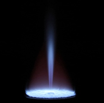
Photograph of the turbulent flame from the experiment.

The centre jet was surrounded by a McKenna burner on which a laminar pilot flame was stabilised. The laminar flame was fed by a
 $\text{CH}_{4}/\text{air}$
mixture at an equivalence ratio of
 $\unicode[STIX]{x1D719}_{c}=0.9$
. The pilot was sufficiently large to shield the jet from the ambient air, avoiding entrainment of the air into the centre jet and ensuring a constant pilot temperature in the region of interest. A photograph of the natural luminosity of the flame from the experiment is shown in figure 1. The bluish colour features
 $\text{CH}^{\ast }$
emission and the maroon colour surrounding the centre jet flame characterises the emission of hot water vapour in the pilot flame.
The pilot temperature estimated from Rayleigh scattering was 1800 K. The adiabatic temperature of the
 $\text{CH}_{4}/\text{air}$
mixture at an equivalence ratio of 0.9 was 2135 K. Therefore, the measured pilot temperature was lower than its adiabatic one, which was primarily due to heat loss from the flame to the water-cooled burner surface.
A calibrated laser Doppler anemometry (LDA) system was employed to measure the axial velocity component. The LDA measurements were focused on stoichiometric flames. The uncertainty of LDA measurements was analysed in Zhou et al. (Reference Zhou, Brackmann, Li, Wang, Petersson, Li, Aldén and Bai2015a
). Simultaneous PLIF measurements of a series of reactive scalars and Rayleigh scattering measurements of temperature, i.e.
 $\text{CH}/\text{CH}_{2}\text{O}/\text{OH}$
,
 $\text{HCO/CH}_{2}\text{O/OH}$
and
 $\text{T}/\text{CH}_{2}\text{O/OH}$
, were carried out. All PLIF images were flat-field corrected and processed with a
 $2\times 2$
pixel median filter to reduce noise. Information about the imaging quality and the signal-to-noise ratio (SNR) of the measured scalars can be found in Zhou et al. (Reference Zhou, Brackmann, Li, Aldén and Bai2015b
). It is noted that the finite SNR and the shot-to-shot variance due to laser intensity fluctuation in the temperature measurements can greatly contaminate the root-mean-square (r.m.s.) temperature results. Therefore, the comparison is not presented in the paper. The measurements thus far were focused on characterisation of turbulence/flame interactions using simultaneous images. Rigorous measurement of species concentrations was not attempted, but is a topic of future work.
3 Numerical simulation
In selecting among the available experiments, our particular interest is in fuel-lean and high
 $Ka$
conditions due to their relevance to lean premixed gas turbines. A lean premixed flame has a larger flame thickness and a lower flame speed than its stoichiometric counterpart, and thus a higher
 $Ka$
can be achieved while keeping the properties of the turbulent flow unchanged. Performing DNS of high
 $Ka$
lean premixed flames provides opportunities to understand various aspects of highly turbulent premixed flames in real combustors. However, such simulations are computationally expensive. With the most powerful supercomputers, it is now feasible to simulate turbulent flames with a jet Reynolds number of
 ${\sim}10\,000$
(Hawkes et al.
Reference Hawkes, Chatakonda, Kolla, Kerstein and Chen2012) using DNS. Based on the above discussion, a high
 $Ka$
flame with a moderate
 $Re$
and a lean
 $\text{CH}_{4}/\text{air}$
mixture is selected among the available experimental conditions for the present study.
The simulation configuration is consistent with the experimental set-up. The jet operates at atmospheric pressure and at a temperature of
 $T_{j}=300$
K. A laminar
 $\text{CH}_{4}/\text{air}$
co-flowing pilot flame having a velocity
 $U_{c}$
of
 $1.8~\text{m}~\text{s}^{-1}$
, a temperature
 $T_{c}$
of 1800 K and an equivalence ratio
 $\unicode[STIX]{x1D719}_{c}$
of 0.9 was used to stabilise the flame. The jet bulk velocity is
 $U_{b}=110~\text{m}~\text{s}^{-1}$
and the jet equivalence ratio is
 $\unicode[STIX]{x1D719}_{j}=0.7$
. In these conditions, the laminar flame velocity
 $S_{L}$
is
 $0.19~\text{m}~\text{s}^{-1}$
, the flame thermal thickness
 $\unicode[STIX]{x1D6FF}_{L}$
is 0.66 mm and the flame time scale
 $\unicode[STIX]{x1D70F}_{L}=\unicode[STIX]{x1D6FF}_{L}/S_{L}$
is 3.4 ms. The jet diameter is
 $D=1.5$
mm and the jet Reynolds number is
 $Re=10\,500$
.
The mean jet axial velocity profile at the inlet is not available from the experimental measurement. In the DNS, it is specified using a power law velocity profile for an axisymmetric fully developed turbulent pipe flow (Yamaguchi Reference Yamaguchi2008). The validity of this profile will be discussed later. A turbulence field is obtained by generating an auxiliary homogeneous isotropic turbulence field based on a prescribed Passot–Pouquet energy spectrum (Passot & Pouquet Reference Passot and Pouquet1987). The turbulent velocity is
 $4~\text{m}~\text{s}^{-1}$
and the integral length scale is 0.75 mm, consistent with the LDA measurement of the experiment. The isotropic turbulence field is then added to the mean inlet velocity using Taylor’s hypothesis. It should be noted that the measured turbulent properties are taken from the flame with
 $U_{b}=110~\text{m}~\text{s}^{-1}$
and
 $\unicode[STIX]{x1D719}_{j}=1.0$
due to the lack of experimental data for the flame with
 $U_{b}=110~\text{m}~\text{s}^{-1}$
and
 $\unicode[STIX]{x1D719}_{j}=0.7$
near the inlet. However, we do not expect that the change in the fuel composition would result in a significant variation in the inflow turbulence.
The Karlovitz number is evaluated at the inlet to be 250. The Damköhler number,
 $Da$
, defined as the ratio of the integral time scale
 $\unicode[STIX]{x1D70F}_{f}$
to the flame time scale
 $\unicode[STIX]{x1D70F}_{L}$
, i.e.
 $Da=\unicode[STIX]{x1D70F}_{f}/\unicode[STIX]{x1D70F}_{L}$
, is 0.054. For the high
 $Ka$
and low
 $Da$
conditions in the present study, all turbulence time scales are smaller than the flame time scale, and the flame is in the broken reaction zones regime (Peters Reference Peters2000).
In the experiment, the flame is attached to the rim of the burner, and the temperature and species profiles are somewhat ambiguous near the burner due to the absence of measurement. For simplicity, the following profile is used to specify a scalar
 $\unicode[STIX]{x1D713}$
(temperature or species mass fraction):
 $$\begin{eqnarray}\unicode[STIX]{x1D713}=\unicode[STIX]{x1D713}_{c}+\frac{\unicode[STIX]{x1D713}_{j}-\unicode[STIX]{x1D713}_{c}}{2}\left(1+\tanh \left(\frac{D/2-r}{\unicode[STIX]{x1D6FF}}\right)\right),\end{eqnarray}$$
where
 $\unicode[STIX]{x1D713}_{j}$
and
 $\unicode[STIX]{x1D713}_{c}$
denote the values of
 $\unicode[STIX]{x1D713}$
in the jet and the pilot respectively. The radial distance is denoted as
 $r$
, and
 $\unicode[STIX]{x1D6FF}$
is a characteristic thickness for the scalar variations. The value of
 $\unicode[STIX]{x1D713}_{c}$
is determined from a chemical equilibrium calculation of a
 $\text{CH}_{4}/\text{air}$
mixture with
 $\unicode[STIX]{x1D719}=0.9$
at a defined temperature of 1800 K, corresponding to the sub-adiabatic temperature estimated from Rayleigh scattering as noted in the last section.
 $\unicode[STIX]{x1D713}_{j}$
is computed based on a
 $\text{CH}_{4}/\text{air}$
mixture with
 $\unicode[STIX]{x1D719}=0.7$
at 300 K. The scalar thickness,
 $\unicode[STIX]{x1D6FF}$
, is specified as
 $0.08D$
for
 $r<D/2$
and the half-width of the burner surface for
 $r>D/2$
to mimic the smooth transition between the pilot and the main jet. A similar inlet profile for scalars was used by Duwig & Dunn (Reference Duwig and Dunn2013) in their large-eddy simulation of highly turbulent piloted premixed flames (Dunn et al.
Reference Dunn, Masri and Bilger2007). This approximation undoubtedly introduces some errors in the near-burner region, but the main focus of this study is on the downstream region, which should be determined mainly by the jet and pilot conditions.
The physical domain for the simulation is large owing to the long flame length:
 $L_{x}\times L_{y}\times L_{z}=48D\times 36D\times 36D$
in the streamwise,
 $x$
, and lateral directions,
 $y$
and
 $z$
, respectively. The grid spacing of the DNS is chosen to adequately resolve both the flame and turbulence structures. A uniform grid spacing of
 $\unicode[STIX]{x0394}x=30~\unicode[STIX]{x03BC}\text{m}$
is used in the streamwise direction
 $x$
, while algebraic stretching is used in the lateral directions
 $y$
and
 $z$
outside of the shear zone. The grid in the
 $y$
(
 $z$
) direction is uniform with
 $\unicode[STIX]{x0394}y~(\unicode[STIX]{x0394}z)=30~\unicode[STIX]{x03BC}\text{m}$
in the region between
 $y/D~(z/D)=-5$
and 5, and gradually stretched outside of this region with a maximum relative stretching rate of 1.9 %. Approximately 22 grid points across
 $\unicode[STIX]{x1D6FF}_{L}$
are obtained with this spatial resolution, which in the present code is sufficient for accurate resolution of the flame structure (Hawkes et al.
Reference Hawkes, Chatakonda, Kolla, Kerstein and Chen2012). In the present high
 $Ka$
case, the resolution of turbulence is more demanding. The Kolmogorov scale, denoted as
 $\unicode[STIX]{x1D702}=(\unicode[STIX]{x1D708}^{3}/\unicode[STIX]{x1D716})^{1/4}$
, has a minimum of
 $10~\unicode[STIX]{x03BC}\text{m}$
in a narrow region near the potential core where the flame does not overlap (here,
 $\unicode[STIX]{x1D716}$
is the kinetic energy dissipation rate). The criterion
 $\unicode[STIX]{x1D702}/\unicode[STIX]{x0394}x>0.5$
(Pope Reference Pope2000) is satisfied elsewhere. Thus, the smallest scales of the turbulent flow are reasonably resolved in the flame region. The resultant number of grids is
 $N_{x}\times N_{y}\times N_{z}=2400\times 900\times 900$
.
To remove artefacts from initialisation, the simulation was first advanced for
 $10\unicode[STIX]{x1D70F}_{j}$
on a half-resolved grid, where
 $\unicode[STIX]{x1D70F}_{j}$
is the flow through time, defined as
 $\unicode[STIX]{x1D70F}_{j}=L_{x}/U_{b}$
. The results were then mapped to the fine grid. The solution was advanced for another
 $10\unicode[STIX]{x1D70F}_{j}$
to provide stationary statistics. It was found that statistical results of the half-resolution run and the production run are very similar, confirming that the resolution is adequate.
The DNS were carried out using the code S3D (Chen et al. Reference Chen, Choudhary, Supinski, DeVries, Hawkes, Klasky, Liao, Ma, Mellor-Crummey and Podhorszki2009), which was originally developed at Sandia National Laboratories. It solves the compressible governing equations of mass continuity, momenta, energy and mass fractions of chemical species including chemical reactions using finite difference methods. The equation sets are solved in a fully coupled way including the two-way interaction of heat release and flow. The code S3D has been used for a number of DNS studies, including early 2D studies of premixed flames (Chen & Im Reference Chen and Im1998; Echekki & Chen Reference Echekki and Chen1999; Hawkes & Chen Reference Hawkes and Chen2006), lifted flames (Yoo, Sankaran & Chen Reference Yoo, Sankaran and Chen2009; Karami, Hawkes & Talei Reference Karami, Hawkes, Talei and Chen2015; Krisman et al. Reference Krisman, Hawkes, Talei, Bhagatwala and Chen2015) and ignitions (Echekki & Chen Reference Echekki and Chen2003), among other topics.
The approach to solve the resulting set of coupled and nonlinear partial differential equations is designed to exploit highly concurrent leadership computing architectures. The governing equations are solved on a conventional three-dimensional structured Cartesian mesh. Spatial differentiation is achieved through eighth-order finite differences (Kennedy & Carpenter Reference Kennedy and Carpenter1994). A tenth-order filter is applied to damp high-wavenumber oscillations. The differentiation and filtering require nine- and eleven-point centred stencils respectively. Time advancement is achieved through a six-stage, fourth-order explicit Runge–Kutta (R–K) method (Kennedy, Carpenter & Lewis Reference Kennedy, Carpenter and Lewis2000), avoiding the expensive all-to-all communication required in implicit methods.
A previously published reduced chemical mechanism for premixed
 $\text{CH}_{4}/\text{air}$
flames with
 $\text{NO}_{x}$
, derived from GRI-Mech3.0, was employed (Lu & Law Reference Lu and Law2008). The skeletal mechanism contains 268 elementary reactions and 44 species, of which 28 species were transported on the DNS grid, including
 $\text{H}_{2}$
, H, O,
 $\text{O}_{2}$
, OH,
 $\text{H}_{2}\text{O}$
,
 $\text{HO}_{2}$
,
 $\text{H}_{2}\text{O}_{2}$
,
 $\text{CH}_{3}$
,
 $\text{CH}_{4}$
, CO,
 $C\text{O}_{2}$
,
 $\text{CH}_{2}\text{O}$
,
 $\text{CH}_{3}\text{OH}$
,
 $\text{C}_{2}\text{H}_{2}$
,
 $\text{C}_{2}\text{H}_{4}$
,
 $\text{C}_{2}\text{H}_{6}$
,
 $\text{CH}_{2}\text{CO}$
,
 $\text{NH}_{2}$
,
 $\text{NH}_{3}$
, NO,
 $\text{NO}_{2}$
,
 $\text{N}_{2}\text{O}$
, HCN, HOCN, HNCO, NCO and
 $\text{N}_{2}$
. The remaining 16 species were identified as quasi-steady state (QSS) species due to their low concentration, high reactivity and short lifetime, including C, CH,
 $\text{CH}_{2}$
,
 $\text{CH}_{2}$
(S), HCO,
 $\text{CH}_{2}\text{OH}$
,
 $\text{CH}_{3}\text{O}$
,
 $\text{C}_{2}\text{H}_{3}$
,
 $\text{C}_{2}\text{H}_{5}$
, HCCO,
 $\text{CH}_{2}\text{CHO}$
, N, NH, NNH, HNO and
 $\text{H}_{2}\text{CN}$
. The QSS algebraic relations were solved analytically without the need for iterations, and the speedup of the simulation was significant due to a reduced number of species transport equations. The resultant mechanism has been validated against the detailed mechanism comprehensively, with very good agreement in a variety of configurations including perfectly stirred reactors, auto-ignition and laminar premixed and non-premixed flames (Lu & Law Reference Lu and Law2008). The mechanism is provided in the supplementary material to the paper at https://doi.org/10.1017/jfm.2017.53.
The simulation was performed on Magnus, a Cray XC-40 located at the Pawsey Supercomputing Centre in Australia, and required 10 million CPU hours on 19 200 Intel Xeon Haswell processor cores for approximately 22 days.
4 Results and discussion
4.1 Comparison with the experiment
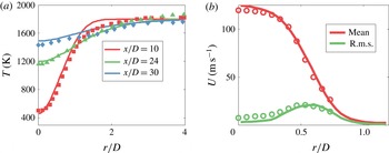
The radial profiles of the mean temperature at
 $x/D=10$
, 24 and 30 are shown in figure 2(a). Along the radial direction, the mean temperature increases from the centreline, and then levels off in the combustion products. Along the streamwise direction, the mean temperature at the centreline increases progressively due to turbulent mixing and heat release. At
 $x/D=30$
, the reactants are almost completely consumed, and the mean temperature begins to approach that of the pilot. The mean temperature is predicted fairly well by the DNS at all locations. A minor discrepancy is found at
 $r/D=1{-}2$
and
 $x/D=10$
. In particular, the DNS slightly overestimates the mean temperature in this region. This could be attributed to a number of factors; for example, the pilot composition could be different from chemical equilibrium, or there might be heat loss from the flame through radiation in the near field, which is not accounted for in the simulation. Moreover, uncertainties in the Rayleigh scattering measurement are inevitable. Despite the near-field discrepancy in the mean temperature, it is seen that further downstream, i.e. at
 $x/D=24$
and 30, the DNS predictions agree with the experimental measurements very well.
(a) Comparison of the mean temperature at
 $x/D=10$
,
 $x/D=24$
and
 $x/D=30$
, and (b) comparison of the mean and r.m.s. axial velocities at
 $x/D=4$
. The solid lines represent the DNS results and the symbols represent the experimental data.

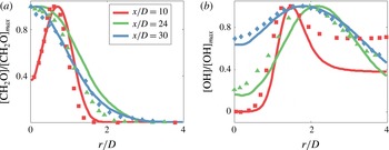
(a) Comparison of the normalised
 $[\text{CH}_{2}\text{O}]$
at
 $x/D=10$
,
 $x/D=24$
and
 $x/D=30$
. (b) Comparison of the normalised [OH] at
 $x/D=10$
,
 $x/D=24$
and
 $x/D=30$
. The solid lines represent the DNS results and the symbols represent the experimental data.

Figure 2(b) shows the radial profiles of the mean and r.m.s. axial velocities at
 $x/D=4$
, the only axial location where the LDA measurements were performed. Very good agreement is obtained between the DNS and the measurements for the mean axial velocity, confirming the validity of the DNS inlet velocity profile. Good agreement is also obtained for the r.m.s. velocity, especially in the shear region where the r.m.s. axial velocity peaks; minor discrepancy is found in the jet region. It should be noted that in the present turbulent jet flame, the shear-generated turbulence is dominant due to the existence of a large mean velocity gradient.
The PLIF signals of
 $\text{CH}_{2}\text{O}$
and OH were corrected to provide estimated species concentrations in the experiment (Zhou et al.
Reference Zhou, Brackmann, Li, Wang, Petersson, Li, Aldén and Bai2015a
). Normalised species concentrations from the DNS and the experiment are compared, i.e. the species profiles are normalised by their peak values (normalisation is necessary because the experiments are not regarded to provide quantitative estimates). Figure 3 shows that good agreement of the normalised
 $[\text{CH}_{2}\text{O}]$
is obtained at all axial locations. The comparison of the normalised [OH] is also good in downstream locations. However, some discrepancies are found at
 $x/D=10$
in the oxidation layer. As mentioned earlier, the OH concentration of the pilot in the DNS is specified based on chemical equilibrium calculation, which might result in a lower value than the real OH concentration in the experiment and be responsible for the upstream discrepancies. This suggests that more accurate inlet boundary conditions from the experiment would be needed to improve the DNS predictions. Interestingly, the discrepancies of OH concentration in the oxidation layer were also found in a numerical and experimental study of laminar propane/air flames (Fayoux et al.
Reference Fayoux, Zähringerc, Gicquela and Rolon2005).
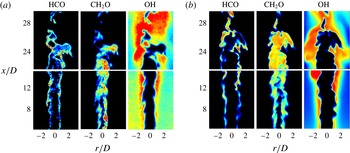
A typical instantaneous snapshot of (a) the simultaneous
 $\text{HCO/CH}_{2}\text{O/OH}$
experimental PLIF images and (b) the
 $\text{HCO/CH}_{2}\text{O/OH}$
molar concentration of the DNS.

Figure 4 shows instantaneous snapshots of species PLIF images of the experiment and species concentrations of the DNS. It should be noted that the species PLIF image intensities may be interpreted qualitatively to be proportional to the species molar concentrations. Panel (a) shows the simultaneous
 $\text{HCO/CH}_{2}\text{O/OH}$
PLIF images and panel (b) shows the
 $\text{HCO/CH}_{2}\text{O/OH}$
molar concentrations of the DNS. For consistency, the filtering from the experiment was also applied to the DNS species concentration fields. While these are random realisations and are not expected to agree one to one, the comparison exhibits qualitatively similar flame structure characteristics. For example, it is readily observed that
 $\text{CH}_{2}\text{O}$
and OH layers are distinct from each other in physical space, while HCO exists in the region between
 $\text{CH}_{2}\text{O}$
and OH. The DNS and the experiment exhibit similar flame wrinkling scales, indicating similar turbulence/chemistry interactions. There are pockets containing reactants pinching off the flame tip. Some of the pockets leave the image without burning completely. However, they are consumed further downstream in the computational domain. The
 $\text{CH}_{2}\text{O}$
and OH layers are seen to be broadened progressively along the streamwise direction, as turbulent eddies are able to penetrate the flame zones and disturb the flame structure. In addition, the layer merging also gives the appearance of a thickened reaction zone. The
 $\text{CH}_{2}\text{O}$
layer is closer to the reactant side where turbulent eddies are stronger, which may penetrate and broaden the
 $\text{CH}_{2}\text{O}$
layer more easily.
An important feature of high
 $Ka$
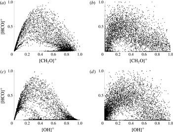
flames is that turbulent convection time scales can be smaller than species reaction time scales; even some short-lived species, such as HCO, can be perturbed by turbulent eddies and redistribute in space. Therefore, a spatial overlap and hence correlation of some species, which is not observed for flames in the flamelet regime, can be expected in high
 $Ka$
flames. The correlations of HCO and
 $\text{CH}_{2}\text{O}/\text{OH}$
are investigated in the present flame, and scatter plots of species concentrations in the DNS and species PLIF signals in the experiment at
 $x/D=24$
are shown in figure 5. The plots are normalised by the maximum value of the corresponding species concentration/signal. It is clear that, in contrast to flamelet behaviour (which would present a single curve), the species distributions are more scattered; moderate concentration of HCO can be found in high
 $\text{OH}/\text{CH}_{2}\text{O}$
concentration regions. It is also seen that the trends of the species correlations are similar in both the DNS and the experiment. It should be noted that the experimental results are more scattered in the plots, which is due to noise in the measurements, as discussed in Wang et al. (Reference Wang, Hawkes, Zhou, Chen, Li and Aldén2017).
Normalised scatter plots of (a,b) [HCO] versus
 $[\text{CH}_{2}\text{O}]$
and (c,d) [HCO] versus [OH] at
 $x/D=24$
. The left-hand plots show the species concentrations of the DNS and the right-hand plots show the species PLIF signals of the experiment.

4.2 Flame stretch
The turbulence/flame interactions are examined using the DNS data. First, the flame stretch statistics are studied. Then, the scalar gradient statistics and flame thickness will be presented in § 4.3. In the present work, the progress variable, c, is defined based on the mass fraction of
 $\text{O}_{2}$
as
 $$\begin{eqnarray}c=(\text{Y}_{\text{O}_{2}}-\text{Y}_{\text{O}_{2},u})/(\text{Y}_{\text{O}_{2},b}-\text{Y}_{\text{O}_{2},u}),\end{eqnarray}$$
where
 $\text{Y}_{\text{O}_{2},u}$
is the
 $\text{O}_{2}$
mass fraction of the reactant while
 $\text{Y}_{\text{O}_{2},b}$
is the
 $\text{O}_{2}$
mass fraction of the pilot. According to this definition, c increases monotonically from zero in the reactant to unity in the pilot stream.
Equation (1.1) can be expanded to have the conventional form involving the tangential strain rate,
 $a_{t}$
, and the curvature stretch,
 $S_{d}\unicode[STIX]{x1D735}\boldsymbol{\cdot }\boldsymbol{n}$
, as follows (Pope Reference Pope1988; Candel & Poinsot Reference Candel and Poinsot1990):
 $$\begin{eqnarray}\frac{\dot{\unicode[STIX]{x1D6FF}A}}{\unicode[STIX]{x1D6FF}A}=\left(\unicode[STIX]{x1D6FF}_{ij}-n_{i}n_{j}\right)\frac{\unicode[STIX]{x2202}{\dot{X}}_{i}}{\unicode[STIX]{x2202}x_{j}}=a_{t}+S_{d}\unicode[STIX]{x1D735}\boldsymbol{\cdot }\boldsymbol{n},\end{eqnarray}$$
where
 $S_{d}$
is the displacement speed and
 $\unicode[STIX]{x1D735}\boldsymbol{\cdot }\boldsymbol{n}$
is the curvature. By definition,
 $\unicode[STIX]{x1D735}\boldsymbol{\cdot }\boldsymbol{n}$
is positive (negative) when the centre of curvature is in the products (reactants). Here, the tangential strain rate,
 $a_{t}$
, is calculated as
 $$\begin{eqnarray}a_{t}=\unicode[STIX]{x1D735}\boldsymbol{\cdot }\boldsymbol{u}-a_{n},\end{eqnarray}$$
where
 $\unicode[STIX]{x1D735}\boldsymbol{\cdot }\boldsymbol{u}$
is the dilatation and
 $a_{n}$
is the normal strain rate given by
 $$\begin{eqnarray}a_{n}=n_{i}\unicode[STIX]{x1D61A}_{ij}n_{j}.\end{eqnarray}$$
Here,
 $n_{i}$
is the
 $i\text{th}$
component of the flame normal vector
 $\boldsymbol{n}$
, defined as
 $$\begin{eqnarray}\boldsymbol{n}=-\unicode[STIX]{x1D735}c/\left|\unicode[STIX]{x1D735}c\right|.\end{eqnarray}$$
By definition,
 $\boldsymbol{n}$
points towards the reactants. The term
 $\unicode[STIX]{x1D61A}_{ij}$
is the strain rate tensor, defined as
 $$\begin{eqnarray}\unicode[STIX]{x1D61A}_{ij}=(\unicode[STIX]{x2202}u_{i}/\unicode[STIX]{x2202}x_{j}+\unicode[STIX]{x2202}u_{j}/\unicode[STIX]{x2202}x_{i})/2.\end{eqnarray}$$
The transport equation for the progress variable is given as
 $$\begin{eqnarray}\unicode[STIX]{x1D70C}\frac{Dc}{Dt}=\dot{\unicode[STIX]{x1D714}}_{c}+\frac{\unicode[STIX]{x2202}}{\unicode[STIX]{x2202}x_{i}}\left(\unicode[STIX]{x1D70C}D_{c}\frac{\unicode[STIX]{x2202}c}{\unicode[STIX]{x2202}x_{i}}\right),\end{eqnarray}$$
where
 $D_{c}$
is the diffusivity of the progress variable and
 $\dot{\unicode[STIX]{x1D714}}_{c}$
is the reaction rate of the progress variable. The progress variable isosurface propagates at the speed
 $S_{d}$
, which denotes the speed of the front relative to the flow normal to the front and is defined as (Gibson Reference Gibson1968; Pope Reference Pope1988)
 $$\begin{eqnarray}S_{d}=\frac{1}{\left|\unicode[STIX]{x1D735}c\right|}\frac{Dc}{Dt}=\frac{\dot{\unicode[STIX]{x1D714}}_{c}}{\unicode[STIX]{x1D70C}\left|\unicode[STIX]{x1D735}c\right|}+\frac{1}{\unicode[STIX]{x1D70C}\left|\unicode[STIX]{x1D735}c\right|}\frac{\unicode[STIX]{x2202}}{\unicode[STIX]{x2202}x_{i}}\left(\unicode[STIX]{x1D70C}D_{c}\frac{\unicode[STIX]{x2202}c}{\unicode[STIX]{x2202}x_{i}}\right).\end{eqnarray}$$
The analysis in this section will exploit surface-averaged quantities. The fine-grained surface average of a quantity
 $Q$
is denoted as (Veynante & Vervisch Reference Veynante and Vervisch2002)
 $$\begin{eqnarray}\left\langle Q\right\rangle _{s}^{\ast }=\frac{\overline{Q\left|\unicode[STIX]{x1D735}c\right|\unicode[STIX]{x1D6FF}(c-c^{\ast })}}{\unicode[STIX]{x1D6F4}^{\ast }},\end{eqnarray}$$
where
 $\unicode[STIX]{x1D6FF}$
is the delta function and
 $\unicode[STIX]{x1D6F4}^{\ast }$
is the fine-grained flame surface density,
 $$\begin{eqnarray}\unicode[STIX]{x1D6F4}^{\ast }=\overline{\left|\unicode[STIX]{x1D735}c\right|\unicode[STIX]{x1D6FF}(c-c^{\ast })}.\end{eqnarray}$$
The ensemble average, denoted as
 $\bar{(\cdots \,)}$
, is performed in time and the homogeneous (azimuthal) direction, so that
 $\unicode[STIX]{x1D6F4}^{\ast }$
and
 $\langle Q\rangle _{s}^{\ast }$
vary in the axial and radial directions. It should be noted that they are also functions of
 $c^{\ast }$
. These definitions can be extended to flames that are not thin (Veynante & Vervisch Reference Veynante and Vervisch2002), as in the present DNS flame. By integrating (4.10) over all isosurface levels, the generalised flame surface density,
 $\unicode[STIX]{x1D6F4}$
, is obtained,
 $$\begin{eqnarray}\unicode[STIX]{x1D6F4}=\int _{0}^{1}\unicode[STIX]{x1D6F4}^{\ast }\,\text{d}c^{\ast }=\int _{0}^{1}\overline{\left|\unicode[STIX]{x1D735}c\right|\unicode[STIX]{x1D6FF}(c-c^{\ast })}\,\text{d}c^{\ast }=\overline{\left|\unicode[STIX]{x1D735}c\right|}.\end{eqnarray}$$
The generalised surface average of
 $Q$
is denoted as
 $$\begin{eqnarray}\left\langle Q\right\rangle _{s}=\frac{\overline{Q\left|\unicode[STIX]{x1D735}c\right|}}{\unicode[STIX]{x1D6F4}}.\end{eqnarray}$$
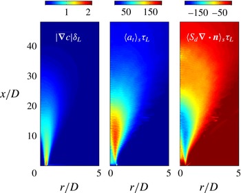
The distribution of
 $\unicode[STIX]{x1D6F4}$
in the
 $x$
–
 $r$
plane is shown in figure 6. It is readily observed that
 $\unicode[STIX]{x1D6F4}$
is high in the upstream region and the distribution is narrow. The magnitude of
 $\unicode[STIX]{x1D6F4}$
decreases and the distribution becomes wider as the flame develops. It should be noted that the integration of
 $\unicode[STIX]{x1D6F4}$
in the radial direction gives the flame area, which will be discussed shortly. Figure 6 also shows the generalised surface-averaged tangential strain rate,
 $\left\langle a_{t}\right\rangle _{s}$
, and curvature stretch,
 $\left\langle S_{d}\unicode[STIX]{x1D735}\boldsymbol{\cdot }\boldsymbol{n}\right\rangle _{s}$
. It is seen that
 $\left\langle a_{t}\right\rangle _{s}$
is mostly positive, producing flame area, while
 $\left\langle S_{d}\unicode[STIX]{x1D735}\boldsymbol{\cdot }\boldsymbol{n}\right\rangle _{s}$
is mostly negative, consuming flame area. This is consistent with studies of statistically 1D planar premixed flames in isotropic turbulence (Trouvé & Poinsot Reference Trouvé and Poinsot1994; Chakraborty & Cant Reference Chakraborty and Cant2005; Hawkes & Chen Reference Hawkes and Chen2005).
The distributions of generalised flame surface density, generalised surface-averaged tangential strain rate and curvature stretch.

For the sake of a compact presentation, the generalised surface averages are also radially integrated such that they vary only with downstream distance. Considering the round jet geometry,
 $$\begin{eqnarray}\left\langle Q\right\rangle _{s,x}(x)=\frac{\displaystyle 2\unicode[STIX]{x03C0}\int _{0}^{\infty }\overline{Q\left|\unicode[STIX]{x1D735}c\right|}r\,\text{d}r\unicode[STIX]{x0394}x}{\displaystyle 2\unicode[STIX]{x03C0}\int _{0}^{\infty }\overline{\left|\unicode[STIX]{x1D735}c\right|}r\,\text{d}r\unicode[STIX]{x0394}x}=\frac{\displaystyle 2\unicode[STIX]{x03C0}\int _{0}^{\infty }\left\langle Q\right\rangle _{s}\unicode[STIX]{x1D6F4}r\,\text{d}r\unicode[STIX]{x0394}x}{\displaystyle 2\unicode[STIX]{x03C0}\int _{0}^{\infty }\unicode[STIX]{x1D6F4}r\,\text{d}r\unicode[STIX]{x0394}x}=\frac{\displaystyle 2\unicode[STIX]{x03C0}\int _{0}^{\infty }\left\langle Q\right\rangle _{s}\unicode[STIX]{x1D6F4}r\,\text{d}r\unicode[STIX]{x0394}x}{A(x)},\end{eqnarray}$$
where
 $A(x)=2\unicode[STIX]{x03C0}\int _{0}^{\infty }\unicode[STIX]{x1D6F4}r\,\text{d}r\unicode[STIX]{x0394}x$
is the flame area at the axial location
 $x$
.
Statistics such as PDF (probability density function), joint PDF and conditional means are also explored to reveal the underlying physics. Consistent with the generalised surface averages described above, the statistics are weighted by
 $|\unicode[STIX]{x1D735}c|$
, unless it is specifically stated otherwise. Three locations are selected to perform the analysis. Their axial distances are
 $x/D=8$
, 16 and 24, and their radial distances correspond to the locations where
 $\unicode[STIX]{x1D6F4}$
is the largest (
 ${\sim}r/D=0.6$
). In order to exclude regions where reaction is unimportant, the statistics are also conditioned on
 $0.5<c<0.9$
(this choice will be shown in § 4.3), except for conditional means which are directly conditioned on the progress variable.
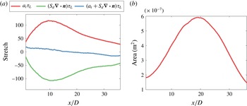
The evolution of the integrated generalised surface-averaged flame stretch and its components along the streamwise direction is shown in figure 7(a). It is first noted that, consistent with the generalised surface-averaged results in figure 6,
 $\left\langle a_{t}\right\rangle _{s,x}$
tends to produce flame area while
 $\left\langle S_{d}\unicode[STIX]{x1D735}\boldsymbol{\cdot }\boldsymbol{n}\right\rangle _{s,x}$
tends to destroy flame area. The value of
 $\left\langle a_{t}\right\rangle _{s,x}$
is relatively small in the near field, which is due to the misalignment of the flame normal with the principal strain rates of the flow, as discussed in Wang, Hawkes & Chen (Reference Wang, Hawkes and Chen2016). The value of
 $\left\langle a_{t}\right\rangle _{s,x}$
increases and reaches its maximum at approximately
 $x/D=10$
. It decreases further downstream, consistent with the increasing characteristic turbulence time scales with downstream distance in this jet flame. Second, it is noted that the magnitude of each term significantly exceeds their sum, suggesting that a quasi-equilibrium exists for creation and destruction of flame area in this region. However, the overall balance of these terms changes with downstream distance. It is observed that, in the upstream region,
 $\left\langle a_{t}\right\rangle _{s,x}$
is larger than
 $\left\langle S_{d}\unicode[STIX]{x1D735}\boldsymbol{\cdot }\boldsymbol{n}\right\rangle _{s,x}$
, and thus the net effect of the flame stretch is the production of flame area. After
 $x/D=20$
, it is seen that
 $\left\langle S_{d}\unicode[STIX]{x1D735}\boldsymbol{\cdot }\boldsymbol{n}\right\rangle _{s,x}$
becomes increasingly dominant over
 $\left\langle a_{t}\right\rangle _{s,x}$
, leading to a net negative stretch, consistent with increasing flame annihilation.
The axial evolution of (a) the integrated generalised surface-averaged flame stretch and its components and (b) the flame area.

The consequences of the flame stretch evolution with downstream distance for the flame area,
 $A(x)$
, are now examined. The evolution of flame area is presented in figure 7(b). It is seen that
 $A(x)$
first increases with downstream distance and peaks near
 $x/D=20$
. Further downstream, it decreases due to the depletion of reactants and the merging of flame segments. The evolution of the flame area is therefore quite consistent with that of the flame stretch. To the best of our knowledge, the spatial development of flame stretch and its correlation with flame area have not been reported before in the literature.
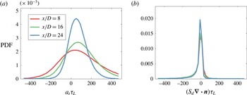
The PDF of (a) the tangential strain rate,
 $a_{t}$
, and (b) the curvature stretch,
 $S_{d}\unicode[STIX]{x1D735}\boldsymbol{\cdot }\boldsymbol{n}$
, at
 $x/D=8$
,
 $x/D=16$
and
 $x/D=24$
.

To further understand the flame stretch components, figure 8 shows the PDF of the tangential strain rate,
 $a_{t}$
, and curvature stretch,
 $S_{d}\unicode[STIX]{x1D735}\boldsymbol{\cdot }\boldsymbol{n}$
, at various downstream locations. The PDF of
 $a_{t}$
is seen to be quite broad with a width that decreases with downstream distance, due to the increasing characteristic turbulence time scales with
 $x/D$
in this jet-type flow. The trend is consistent with that observed for increasing Damköhler numbers in DNS of statistically 1D planar premixed flames (Chakraborty & Swaminathan Reference Chakraborty and Swaminathan2007). The PDF of
 $S_{d}\unicode[STIX]{x1D735}\boldsymbol{\cdot }\boldsymbol{n}$
has a quite different character, with most of the flame surface exhibiting low stretch values, while there is a very long tail with small amounts of flame surface exhibiting very large negative stretch. As noted in previous work on statistically 1D planar premixed flames (Hawkes & Chen Reference Hawkes and Chen2005), this trend is consistent with the concept of scale separation in turbulent flows, wherein significant dissipation (in this case, of the flame area) occurs in very small-scale features (in this case, features that have very large curvatures).
The joint PDF of (a) the tangential strain rate and the curvature, and (b) the flame stretch and the curvature, at
 $x/D=24$
, where the conditional mean is denoted by the black solid line.

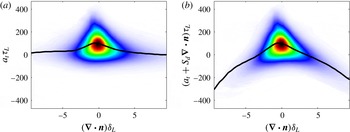
Strain rate and curvature are not independent quantities, however. To examine this, figure 9 shows the joint PDF of tangential strain rate and curvature (figure 9
a) and net flame stretch and curvature (figure 9
b), and the conditional means of each quantity on curvature at
 $x/D=24$
. Figure 9(a) shows that high positive tangential strain rate regions generally have low curvatures while high curvature regions generally have low strains, a finding that has been reported before for low Damköhler number statistically 1D planar premixed flames (Chakraborty & Cant Reference Chakraborty and Cant2005). Although the response of the curvature to strain depends on the alignment of their respective principal axes, intuition suggests that high tangential strain rate of a surface should tend to smooth wrinkles in the surface, which is exactly what is observed. The net flame stretch presents a somewhat different picture. Figure 9(b) shows that the strong net positive stretch regions consistently occur in regions that have low curvature magnitudes, which by comparison with figure 9(a) are deduced to be high positive strain regions. However, the high net negative stretch regions occur most often in regions of large curvature, the sign of the curvature being unimportant. Since curvature stretch is given by
 $S_{d}\unicode[STIX]{x1D735}\boldsymbol{\cdot }\boldsymbol{n}$
, but both large positive and large negative curvatures still lead to high negative stretch, it is deduced that the displacement speed and curvature must be strongly correlated.
To investigate the importance and nature of this correlation, the curvature stretch term,
 $S_{d}\unicode[STIX]{x1D735}\boldsymbol{\cdot }\boldsymbol{n}$
, is further studied. Previous modelling of flames in the flamelet regime has assumed that the displacement speed and the curvature are not correlated, and hence
 $$\begin{eqnarray}\left\langle S_{d}\unicode[STIX]{x1D735}\boldsymbol{\cdot }\boldsymbol{n}\right\rangle _{s}\approx \left\langle S_{d}\right\rangle _{s}\left\langle \unicode[STIX]{x1D735}\boldsymbol{\cdot }\boldsymbol{n}\right\rangle _{s}.\end{eqnarray}$$
However, in highly turbulent flames, this assumption is no longer appropriate, and the correlation must be accounted for. To quantify the importance of this correlation, the following decomposition of
 $\langle S_{d}\unicode[STIX]{x1D735}\boldsymbol{\cdot }\boldsymbol{n}\rangle _{s}$
is proposed:
 $$\begin{eqnarray}\left\langle S_{d}\unicode[STIX]{x1D735}\boldsymbol{\cdot }\boldsymbol{n}\right\rangle _{s}=\left\langle S_{d}\right\rangle _{s}\left\langle \unicode[STIX]{x1D735}\boldsymbol{\cdot }\boldsymbol{n}\right\rangle _{s}+(\left\langle S_{d}\unicode[STIX]{x1D735}\boldsymbol{\cdot }\boldsymbol{n}\right\rangle _{s}-\left\langle S_{d}\right\rangle _{s}\left\langle \unicode[STIX]{x1D735}\boldsymbol{\cdot }\boldsymbol{n}\right\rangle _{s}),\end{eqnarray}$$
where the first term gives the combined action of the mean flame speed with the mean curvature while the second accounts for flame speed–curvature correlations. Previous theoretical analysis for the thin reaction zones regime (Peters Reference Peters1999) suggested that these correlations could be approximated by breaking down the
 $S_{d}$
contributions into different components that have different curvature responses. Here,
 $S_{d}$
is decomposed into its reaction (
 $S_{d,r}$
), normal diffusion (
 $S_{d,n}$
) and curvature (
 $S_{d,c}$
) components as (Echekki & Chen Reference Echekki and Chen1999)
 $$\begin{eqnarray}S_{d}=S_{d,r}+S_{d,n}+S_{d,c}=\frac{\dot{\unicode[STIX]{x1D714}}_{c}}{\unicode[STIX]{x1D70C}|\unicode[STIX]{x1D735}c|}+\frac{1}{\unicode[STIX]{x1D70C}|\unicode[STIX]{x1D735}c|}\frac{\unicode[STIX]{x2202}}{\unicode[STIX]{x2202}n}\left(\unicode[STIX]{x1D70C}D_{c}\frac{\unicode[STIX]{x2202}c}{\unicode[STIX]{x2202}n}\right)-D_{c}\unicode[STIX]{x1D735}\boldsymbol{\cdot }\boldsymbol{n},\end{eqnarray}$$
where
 $n$
is the distance along the flame normal direction. The sum of the reaction and normal diffusion components of the displacement speed is also known as kinematic restoration,
 $S_{d,r+n}$
(Peters Reference Peters1999). Therefore,
 $S_{d}\unicode[STIX]{x1D735}\boldsymbol{\cdot }\boldsymbol{n}$
can be recast as
 $$\begin{eqnarray}S_{d}\unicode[STIX]{x1D735}\boldsymbol{\cdot }\boldsymbol{n}=S_{d,r+n}\unicode[STIX]{x1D735}\boldsymbol{\cdot }\boldsymbol{n}-D_{c}(\unicode[STIX]{x1D735}\boldsymbol{\cdot }\boldsymbol{n})^{2}.\end{eqnarray}$$
Accordingly,
 $\langle S_{d}\unicode[STIX]{x1D735}\boldsymbol{\cdot }\boldsymbol{n}\rangle _{s}$
can also be written as
 $$\begin{eqnarray}\left\langle S_{d}\unicode[STIX]{x1D735}\boldsymbol{\cdot }\boldsymbol{n}\right\rangle _{s}=\left\langle S_{d,r+n}\unicode[STIX]{x1D735}\boldsymbol{\cdot }\boldsymbol{n}\right\rangle _{s}-\left\langle D_{c}(\unicode[STIX]{x1D735}\boldsymbol{\cdot }\boldsymbol{n})^{2}\right\rangle _{s},\end{eqnarray}$$
where both terms on the right-hand side may show correlations with curvature.
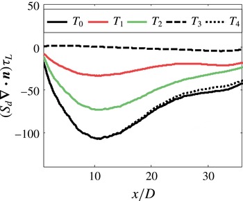
Following (4.13), the integrated generalised surface averages of the above-mentioned quantities are studied. The evolution of
 $\left\langle S_{d}\unicode[STIX]{x1D735}\boldsymbol{\cdot }\boldsymbol{n}\right\rangle _{s,x}$
and the relevant terms is shown in figure 10. It is first noted that the term due to correlation of flame speed with curvature,
 $\left\langle S_{d}\unicode[STIX]{x1D735}\boldsymbol{\cdot }\boldsymbol{n}\right\rangle _{s,x}-\left\langle S_{d}\right\rangle _{s,x}\left\langle \unicode[STIX]{x1D735}\boldsymbol{\cdot }\boldsymbol{n}\right\rangle _{s,x}$
, is strongly dominant over
 $\left\langle S_{d}\right\rangle _{s,x}\left\langle \unicode[STIX]{x1D735}\boldsymbol{\cdot }\boldsymbol{n}\right\rangle _{s,x}$
across almost the entire flame. It is also clear that
 $-\langle D_{c}(\unicode[STIX]{x1D735}\boldsymbol{\cdot }\boldsymbol{n})^{2}\rangle _{s,x}$
is dominant over
 $\left\langle S_{d,r+n}\unicode[STIX]{x1D735}\boldsymbol{\cdot }\boldsymbol{n}\right\rangle _{s,x}$
. This is because the curvature component of the displacement speed,
 $S_{d,c}$
, is always negatively correlated with curvature, contributing significantly to
 $\left\langle S_{d}\unicode[STIX]{x1D735}\boldsymbol{\cdot }\boldsymbol{n}\right\rangle _{s,x}$
. However, it is certainly not the case that the curvature correlation of
 $S_{d,r+n}$
can be ignored, and indeed in the downstream region, the contribution of
 $\left\langle S_{d,r+n}\unicode[STIX]{x1D735}\boldsymbol{\cdot }\boldsymbol{n}\right\rangle _{s,x}$
to the surface-averaged flame stretch increases.
The axial evolution of the integrated generalised surface-averaged curvature stretch term:
 $T_{0}$
,
 $\left\langle S_{d}\unicode[STIX]{x1D735}\boldsymbol{\cdot }\boldsymbol{n}\right\rangle _{s,x}$
;
 $T_{1}$
,
 $\left\langle S_{d,r+n}\unicode[STIX]{x1D735}\boldsymbol{\cdot }\boldsymbol{n}\right\rangle _{s,x}$
;
 $T_{2}$
,
 $-\langle D_{c}(\unicode[STIX]{x1D735}\boldsymbol{\cdot }\boldsymbol{n})^{2}\rangle _{s,x}$
;
 $T_{3}$
,
 $\left\langle S_{d}\right\rangle _{s,x}\left\langle \unicode[STIX]{x1D735}\boldsymbol{\cdot }\boldsymbol{n}\right\rangle _{s,x}$
;
 $T_{4}$
,
 $\left\langle S_{d}\unicode[STIX]{x1D735}\boldsymbol{\cdot }\boldsymbol{n}\right\rangle _{s,x}-\left\langle S_{d}\right\rangle _{s,x}\left\langle \unicode[STIX]{x1D735}\boldsymbol{\cdot }\boldsymbol{n}\right\rangle _{s,x}$
.

4.3 Flame thickness
In the following, we address the question: what is the influence of turbulence on the flame thickness and the corresponding scalar gradients? The thicknesses of several species layers were presented in figure 4. In particular, the
 $\text{CH}_{2}\text{O}$
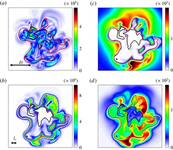
and OH layers are increasingly broadened with increasing downstream distance. The flame structure is further investigated to show the flame thickness. Figure 11 displays the instantaneous distributions of the vorticity, heat release rate, and OH and CO mass fractions at the axial location
 $x/D=20$
. Of particular interest is the reaction zone, where chemical reactions occur and heat is released. The reaction zone is defined as the region where the heat release rate exceeds 35 % of its local maximum value, spanning approximately
 $c^{\ast }=0.5$
–0.9. The distance between
 $c^{\ast }=0.5$
and 0.9 for the unstrained laminar flame, denoted
 $l_{c}$
, is also shown for comparison. It is readily observed that turbulent eddies enter into and disturb the reaction zone. There are regions where the thickness of the reaction zone is an order of magnitude larger than its laminar counterpart. The distribution of CO is particularly disturbed by turbulence, a feature of the broken reaction zones regime. On the other hand, the distribution of OH is less affected, as OH has a higher concentration on the product side where turbulence is weaker due to the higher viscosity in the products. Following these observations, quantitative analyses of the turbulent flame thickness are performed next.
Instantaneous distributions of the (a) vorticity (
 $\text{s}^{-1}$
), (b) heat release rate (
 $\text{J}~\text{m}^{-3}~\text{s}$
), (c) OH mass fraction and (d) CO mass fraction at
 $x/D=20$
. The isolines of the progress variable are delineated as follows: (black)
 $c^{\ast }=0.5$
, (red)
 $c^{\ast }=0.8$
and (white)
 $c^{\ast }=0.9$
. The nozzle diameter,
 $D$
, and the distance between
 $c^{\ast }=0.5$
and 0.9 in the unstrained laminar flame,
 $l_{c}$
, are also added for reference.

The thickness of the turbulent flame is discussed more quantitatively in terms of the scalar gradient magnitude,
 $|\unicode[STIX]{x1D735}c|$
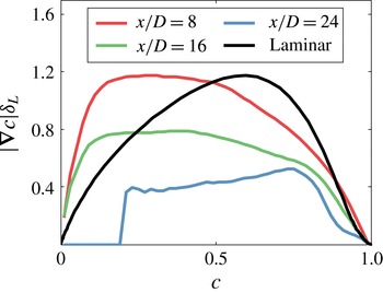
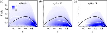
, which represents a reciprocal flame thickness. Figure 12 shows
 $|\unicode[STIX]{x1D735}c|$
conditionally averaged on c at various downstream locations. (It should be noted that the results in figures 12–14 are not weighted by
 $|\unicode[STIX]{x1D735}c|$
.) The profile of
 $|\unicode[STIX]{x1D735}c|$
of the unstrained laminar premixed flame is also plotted. At
 $x/D=8$
,
 $|\unicode[STIX]{x1D735}c|$
of the DNS is higher than that of the unstrained laminar flame for
 $c<0.5$
. On the other hand,
 $|\unicode[STIX]{x1D735}c|$
of the DNS is lower than that of the laminar flame for
 $c>0.5$
. It is worth noting that the structure of the turbulent flame is expected to be different from that of the unstrained laminar flame due to the existence of pilot, mean shear and complex turbulence/flame interactions. A detailed comparison of the turbulent flame and strained laminar flames is a subject of future work. As the flame develops downstream, the mean strain relaxes while small-scale turbulence progressively penetrates the flame, modifying the inner layer of the flame at high local
 $Ka$
(
 $100<Ka$
). At
 $x/D=24$
, the flame is considerably broadened and the mean flame thickness is approximately
 $2\unicode[STIX]{x1D6FF}_{L}$
. Importantly, this thickening is also observed in the reaction zone.
The surface density function
 $|\unicode[STIX]{x1D735}c|$
conditionally averaged on the progress variable.

It is interesting to observe the large
 $|\unicode[STIX]{x1D735}c|$
region of the preheat zone upstream, which might at first consideration be an unexpected feature for high
 $Ka$
where on-average flame broadening is expected. In order to understand this behaviour, first the instantaneous/mean flame structure and then the joint PDF of
 $c$
and
 $|\unicode[STIX]{x1D735}c|$
are examined. A distance function,
 $L_{D}$
, is introduced, which represents the spatial distance with respect to the flame surface (Peters Reference Peters2000; Sankaran et al.
Reference Sankaran, Hawkes, Yoo and Chen2015). The distance function
 $L_{D}$
is defined such that at each point in the computational domain it signifies the shortest normal distance to the flame surface, computed by solving the Eikonal equation,
 $$\begin{eqnarray}|\unicode[STIX]{x1D735}L_{D}|=1.\end{eqnarray}$$
The distance function
 $L_{D}$
is set to zero on the
 $c^{\ast }=0.8$
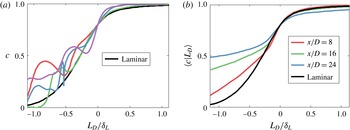
isosurface (this is the point of maximum heat release in a freely propagating laminar flame), negative in the reactants and positive in the products. Four representative instantaneous profiles of the progress variable versus the distance function at
 $x/D=8$
are shown in figure 13(a). It is seen that the instantaneous profiles are significantly perturbed by turbulence, and the progress variable does not increase monotonically with the distance function as it does in the laminar flame. This is because peninsular-like structures and/or pockets of partially reacted gas are formed in the preheat zone due to the interactions of small-scale turbulent eddies and flame, increasing the local scalar gradient and giving the appearance of a locally ‘thinner’ preheat zone as measured by the magnitude of the scalar gradient. In contrast, figure 13(b) shows the profiles of the progress variable conditionally averaged on the distance function. It is seen that the preheat zone of the mean flame structure is, however, thicker in the turbulent flame compared with the laminar flame. It should be noted that, due to strong turbulent mixing between the reactants and products, the mean progress variable of the reactants increases with downstream distance.
(a) Four representative instantaneous profiles of the progress variable versus the distance function at
 $x/D=8$
. (b) The progress variable conditionally averaged on the distance function at
 $x/D=8$
,
 $x/D=16$
and
 $x/D=24$
.

Figure 14 shows the joint PDF of the progress variable and the surface density function at various downstream locations. It is readily seen that the distribution of the surface density function is broad, especially at
 $x/D=8$
, where the local flame can be very thin (as measured by the scalar gradient). It will be shown later that the local flame thinning (increasing scalar gradient) corresponds to large and positive tangential strain rate. It is suggested that the average of
 $|\unicode[STIX]{x1D735}c|$
is the result of the competition between large
 $|\unicode[STIX]{x1D735}c|$
induced by small-scale flame structures and small
 $|\unicode[STIX]{x1D735}c|$
due to the flame thickening. The former plays an important role in the preheat zone upstream, while the latter is dominant downstream as the flame is increasingly thickened.
Joint PDF of the progress variable and the surface density function. The white line denotes the conditionally averaged surface density function of the DNS and the black line denotes the unstrained laminar premixed flame result.

As discussed earlier, the balance equation for
 $|\unicode[STIX]{x1D735}c|$
provides a framework for understanding the flame thinning/thickening as isoscalar surfaces are brought together or separated by turbulent straining and self-propagation. Following Sankaran et al. (Reference Sankaran, Hawkes, Chen, Lu and Law2007), equation (1.1) can be expanded as
 $$\begin{eqnarray}\frac{\dot{\left|\unicode[STIX]{x1D735}c\right|}}{\left|\unicode[STIX]{x1D735}c\right|}=-n_{i}n_{j}\frac{\unicode[STIX]{x2202}{\dot{X}}_{i}}{\unicode[STIX]{x2202}x_{j}}=-(a_{n}+\unicode[STIX]{x2202}S_{d}/\unicode[STIX]{x2202}n).\end{eqnarray}$$
Using the decomposition of the displacement speed, equation (4.20) can be recast as
 $$\begin{eqnarray}\frac{\dot{\left|\unicode[STIX]{x1D735}c\right|}}{\left|\unicode[STIX]{x1D735}c\right|}=-(a_{n}+\unicode[STIX]{x2202}S_{d,r+n}/\unicode[STIX]{x2202}n+\unicode[STIX]{x2202}S_{d,c}/\unicode[STIX]{x2202}n).\end{eqnarray}$$
In the following, the effects of the terms representing the normal strain rate (
 $a_{n}$
), kinematic restoration (
 $\unicode[STIX]{x2202}S_{d,r+n}/\unicode[STIX]{x2202}n$
) and curvature (
 $\unicode[STIX]{x2202}S_{d,c}/\unicode[STIX]{x2202}n$
) on the flame thickness are analysed. It should be noted here that positive-valued terms act as sinks for
 $|\unicode[STIX]{x1D735}c|$
, and vice versa.
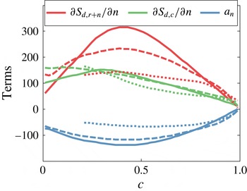
Budget of the source terms in the balance equation for
 $|\unicode[STIX]{x1D735}c|$
conditionally averaged on the progress variable. The terms are non-dimensionalised using
 $\unicode[STIX]{x1D70F}_{L}$
. Solid line,
 $x/D=8$
; dashed line,
 $x/D=16$
; dotted line,
 $x/D=24$
.

Figure 15 shows the budget of various terms conditioned on c. It is obvious that the kinematic restoration term and the curvature term are positive, leading to lower scalar gradients and a thicker flame. On the other hand, the normal strain rate term is negative, contributing to a source for
 $|\unicode[STIX]{x1D735}c|$
and a locally thinner flame. Overall, the net balance is in favour of thickening of the flame across all values of
 $c$
. This result is important in that it reveals the mechanism for the flame thickening as the flame traverses downstream. In particular, the displacement speed of an isoscalar surface decreases monotonically from reactants to products, causing a larger distance between two isoscalar surfaces. Negative normal strain rate tends to bring the isoscalar surfaces together. However, its magnitude is small compared with the terms involving normal gradients of the flame speed (
 $\unicode[STIX]{x2202}S_{d,r+n}/\unicode[STIX]{x2202}n+\unicode[STIX]{x2202}S_{d,c}/\unicode[STIX]{x2202}n$
). This scenario is in contrast to the result of Dopazo et al. (Reference Dopazo, Cifuentes, Martín and Jiménez2015), who reported a positive normal strain rate term and a negative flame speed-gradient term in a low
 $Ka$
flame.
To further understand the influence of turbulence on disturbing the inner structure of the flame, the effects of the tangential strain rate,
 $a_{t}$
, and curvature,
 $\unicode[STIX]{x1D735}\boldsymbol{\cdot }\boldsymbol{n}$
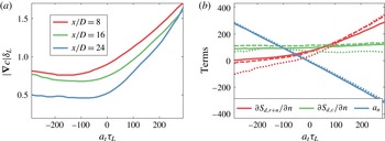
, on the flame thickness are investigated. Figure 16(a) shows
 $|\unicode[STIX]{x1D735}c|$
conditionally averaged on
 $a_{t}$
. It is clear that
 $|\unicode[STIX]{x1D735}c|$
increases with
 $a_{t}$
for positive
 $a_{t}$
. For negative
 $a_{t}$
, the scalar gradient magnitude is low and insensitive to
 $a_{t}$
. Figure 16(b) indicates that at positive
 $a_{t}$
, the normal strain rate term becomes the dominant source for
 $|\unicode[STIX]{x1D735}c|$
, which produces scalar gradients and is responsible for the local flame thinning. Meanwhile, at negative
 $a_{t}$
, the normal strain rate term and, to a lesser extent, the curvature term tend to dissipate scalar gradient and locally thicken the flame.
The influence of curvature is finally assessed. Figure 17(a) shows
 $|\unicode[STIX]{x1D735}c|$
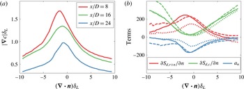
conditionally averaged on curvature. In general, the flame is thicker as the curvature magnitude increases (both negative and positive). This observation is consistent with the DNS of Sankaran et al. (Reference Sankaran, Hawkes, Chen, Lu and Law2007) and the experiment of Tamadonfar & Gülder (Reference Tamadonfar and Gülder2015). The flames that are near zero curvature coincide with regions of highly negative normal strain rate (figure 17
b) and are locally thinned. The budget analysis of figure 17(b) indicates that the dominant source at large curvatures is the positive curvature term, which separates isoscalar surfaces and thickens the flame. At small curvatures, the normal strain rate term is seen to be counteracted by the kinematic restoration term.
(a) The surface density function
 $|\unicode[STIX]{x1D735}c|$
conditionally averaged on the tangential strain rate. (b) Budget of the source terms in the balance equation for
 $|\unicode[STIX]{x1D735}c|$
conditionally averaged on the tangential strain rate. The terms are non-dimensionalised using
 $\unicode[STIX]{x1D70F}_{L}$
. Solid line,
 $x/D=8$
; dashed line,
 $x/D=16$
; dotted line,
 $x/D=24$
.

(a) The surface density function
 $|\unicode[STIX]{x1D735}c|$
conditionally averaged on the curvature. (b) Budget of the source terms in the balance equation for
 $|\unicode[STIX]{x1D735}c|$
conditionally averaged on the curvature. The terms are non-dimensionalised using
 $\unicode[STIX]{x1D70F}_{L}$
. Solid line,
 $x/D=8$
; dashed line,
 $x/D=16$
; dotted line,
 $x/D=24$
.

5 Conclusions
Direct numerical simulations of an experimental lean premixed jet flame at high Karlovitz number were simulated using a detailed chemistry model. Results for mean temperature/species were compared quantitatively with the experiments and good agreement was obtained. Qualitative comparisons for key species including HCO,
 $\text{CH}_{2}\text{O}$
and OH were also very good, with key features such as locally reduced concentrations corresponding to extinction and substantial thickening being reproduced in the DNS.
The DNS were examined from the perspective of the flame area and local thickness of progress variable fields, which together can characterise the volume of reacting material. The evolutions of these two quantities are closely connected, with their rates of change in an isosurface following reference frame being given by the tangential and normal gradients of velocities of points on the isosurface respectively.
The analysis first discussed the flame stretch, finding, in agreement with previous studies of statistically 1D planar premixed flames, that the tangential strain rate on-average produces flame area while the curvature stretch destroys it. These individual terms were found to be large compared with their sum, with the balance shifting from the former to the latter with increasing downstream distance. A joint analysis of the local flame stretch with curvature demonstrated that flame area tends to be produced in high positive strain, low curvature regions while it is destroyed in low tangential strain, high curvature regions. The curvature stretch was found to be dominated by low probability regions that have very large negative stretch rates. Further analysis of the curvature stretch showed that it is fundamentally driven by correlations of the flame speed with the curvature. These correlations are mostly attributable to the tangential diffusion of the progress variable, which gives rise to a stretch proportional to the curvature squared. However, contributions from the reaction rate and normal diffusion of the progress variable become more significant with increasing downstream distance.
The internal structure of the flame was examined, and substantial flame thickening was observed downstream. Interestingly, local thinning of the preheat zone upstream, as measured by
 $|\unicode[STIX]{x1D735}c|$
, is significant due to the interactions of small-scale turbulent eddies and the flame. Evidence was presented showing that turbulent eddies enter into and disturb the reaction zone. The budget analyses of
 $|\unicode[STIX]{x1D735}c|$
showed that the normal gradient of flame propagation, i.e. the normal derivative of the displacement speed, dominates over the normal strain rate term across the progress variable space, dissipating scalar gradient and thickening the flame as it traverses downstream. Local flame thinning (as indicated by large gradients) was observed in regions with largely positive values of the tangential strain rate, where the largely negative values of the normal strain rate produce scalar gradient and thin the flame. Flame thickening is most evident in highly curved regions due to the curvature term.
Connecting these two analyses, this article shows that high positive tangential strain regions generally correspond with low curvature regions; these regions tend to be positively stretched and are relatively thinner compared with other regions. High curvature magnitude regions (both positive and negative) generally correspond with lower tangential strain; these regions are in net negatively stretched and thickened substantially.
Acknowledgements
The work at UNSW Australia was supported by the Australian Research Council (ARC). The work at Sandia National Laboratories was supported by the Division of Chemical Sciences, Geosciences and Biosciences, the Office of Basic Energy Sciences, the US Department of Energy (DOE). Sandia National Laboratories is a multiprogram laboratory operated by Sandia Corporation, a Lockheed Martin Company, for the US Department of Energy under contract De-AC04-94-AL85000. The work at Lund University was supported by the Swedish Energy Agency. The DNS runs were carried out under the Petascale Pioneers Program and National Computational Merit Allocation Scheme at the Pawsey Supercomputing Centre with funding from the Australian Government and the Government of Western Australia.
Supplementary material
Supplementary material is available at https://doi.org/10.1017/jfm.2017.53.