1 Introduction
Buoyancy driven convection plays a central role in a great number of geophysical processes occurring at large and medium scales (convective flows in the mantle, volcanoes, fires, hydrothermal vents). Because mixing and dispersion issues motivated the very first studies on the topic, plume dynamics has been extensively addressed in the case of sustained turbulent regimes. The now classical entrainment assumption introduced in classical works by Batchelor (Reference Batchelor1954) and Morton, Taylor & Turner (Reference Morton, Taylor and Turner1956) still generates new developments (Kaminski, Tait & Carazzo Reference Kaminski, Tait and Carazzo2005; Carazzo, Kaminski & Tait Reference Carazzo, Kaminski and Tait2006, Reference Carazzo, Kaminski and Tait2010). Here, because the typical size of the system and fluid velocities are small (a few centimetres and a few millimetres per second), the Reynolds number is of the order of a few hundreds. Consequently, the confined plumes under consideration in the present study are not turbulent.
Analytical solutions for laminar plumes emitted by a point source have been first obtained by Yih (Reference Yih1951), Fujii (Reference Fujii1963) and Pera & Gebhart (Reference Pera and Gebhart1971) for fixed values of Prandtl numbers equal to 1 and 2. The case of an infinite Prandtl number has been solved later by Worster (Reference Worster1986) in the case of an infinite medium and by Whittaker & Lister (Reference Whittaker and Lister2006a ) in the case of a semi-infinite medium (i.e. over a horizontal plane). Finally, extended sources of buoyancy have been considered by Umemura & Busse (Reference Umemura and Busse1989), Whittaker & Lister (Reference Whittaker and Lister2006b ) and Nadal et al. (Reference Nadal, Meunier, Pouligny and Laurichesse2013). The radial confinement of the plume has been studied within the scope of geological applications where the variation of viscosity with temperature leads to narrow conduit structures with high-velocity cores (see e.g. Olson, Schubert & Anderson Reference Olson, Schubert and Anderson1993). This viscosity driven confinement generally leads to the same scalings in Rayleigh number for the core velocity as that resulting from direct mechanical confinement (Umemura & Busse Reference Umemura and Busse1989; Nadal et al. Reference Nadal, Meunier, Pouligny and Laurichesse2013).
In general, whereas numerous studies have been devoted to either laminar or turbulent buoyant plumes in confined environments, not many have addressed the mechanisms of transition from steady to unsteady regimes (Cetegen, Dong & Soteriou Reference Cetegen, Dong and Soteriou1998; Maxworthy Reference Maxworthy1999; Soteriou, Dong & Cetegen Reference Soteriou, Dong and Cetegen2002; Williams et al. Reference Williams, Shaddix, Schefer and Desgroux2007). As pointed out by Lopez & Marques (Reference Lopez and Marques2013), a general understanding of such a transitional process between steady axisymmetric laminar plumes and turbulent plumes is still missing probably because the destabilisation mechanisms at stake strongly depend on the details of the configuration (geometry and boundary conditions). These configurations fall broadly into two categories.
In the first case, the plume is generated by a buoyant jet with a fixed rate of buoyancy. This is for example the case of a helium round jet in air, as studied experimentally by Subbarao & Cantwell (Reference Subbarao and Cantwell1992), Cetegen & Kasper (Reference Cetegen and Kasper1996) and Cetegen et al. (Reference Cetegen, Dong and Soteriou1998). The jet becomes unstable with respect to an axisymmetric puffing (varicose) instability whose frequency varies as
 $Ri^{0.38}$
(where the Richardson number
 $Ri$
is based on the density difference and the jet diameter and velocity). These observations were corroborated by the direct numerical simulations results of Jiang & Luo (Reference Jiang and Luo2000) and of Satti & Agrawal (Reference Satti and Agrawal2006). This is also consistent with the recent theoretical analysis of Chakravarthy, Lesshafft & Huerre (Reference Chakravarthy, Lesshafft and Huerre2018) based on global modes. However, the local stability analysis by Chakravarthy, Lesshafft & Huerre (Reference Chakravarthy, Lesshafft and Huerre2015) found that the dominant and only absolutely unstable perturbation is helical rather than axisymmetric. Experiments have also been performed by Pesci, Porter & Goldstein (Reference Pesci, Porter and Goldstein2003) in a Hele-Shaw cell where a salted water jet was injected from a point source into a stably stratified environment. They observed an asymmetric sinuous instability rather than a varicose instability. Pesci’s first interpretation of this buckling instability relied on a two-dimensional Kelvin–Helmholtz instability scenario while subsequent theoretical works by Lombardi et al. (Reference Lombardi, Caulfield, Cossu, Pesci and Goldstein2011) provided a quite different explanation of Pesci’s observations based on vorticity enhancement by horizontal density gradient effects. In these studies, the high values of the Schmidt number is a key ingredient of the instability. Lombardi et al. (Reference Lombardi, Caulfield, Cossu, Pesci and Goldstein2011) also obtained a subdominant varicose mode similar to the instability that we observe in three dimensions. However, the buoyant jet is injected into a pre-existing stratified environment whereas, in our study, stratification builds up as the carbon dioxide dissolves into the tube. Furthermore, in Pesci’s experiments and Lombardi’s theoretical study, the buoyancy flux is fixed and steady whereas in our experiments the buoyancy flux increases with the fluid velocity and thus oscillates in the unsteady regime.
Alternatively, the plume can be generated without recourse to any jet by a simple condition of buoyancy at the boundary. For instance thermal plumes are classically created by imposing a fixed temperature at a point source (the spatial extent of which is often poorly known). The boundary conditions of thermal buoyancy experiments are thus closer to the configuration studied in this paper (despite the smaller values of the Prandtl number). Torrance, Orloff & Rockett (Reference Torrance, Orloff and Rockett1969) performed an experimental study of a confined thermal plume generated in water by a localised source (with a Prandtl number equal to 7). Corresponding numerical simulations were presented by Torrance & Rockett (Reference Torrance and Rockett1969) in a companion paper. Experiments and numerical simulations revealed the presence of axisymmetric varicose instabilities, while simulations failed to accurately compute the critical Rayleigh number. Later, Torrance (Reference Torrance1979) added a background stratification; he observed a quasi-steady regime but could not observe the unstable regime because he was not able to reach a sufficiently high Rayleigh number. Lopez & Marques (Reference Lopez and Marques2013) performed numerical simulations without background stratification and with a small radial dimension of the buoyancy source in a confined geometry (inside a finite-height cylinder) with a Prandtl number equal to 7. They observed an axisymmetric varicose instability above a critical height-based Rayleigh number equal to
 $5.4\times 10^{7}$
. This instability was followed by a subsequent breaking of the axisymmetry at larger Rayleigh numbers. Kimura & Bejan (Reference Kimura and Bejan1983) did similar (but unstratified) experiments in air (where the Prandtl number was equal to 0.7) in a larger container. They found that the instability is not axisymmetric and occurs as a buckling of the plume rather than a varicose puffing sequence. These asymmetric instabilities were later explained theoretically by Yang (Reference Yang1992). Despite the apparent strong similarities between these configurations and our experimental study, there are still major differences. First, they impose the temperature on all boundaries (leading to a stationary base state) whereas we have no flux of buoyancy on the sides and the bottom wall (leading to a filling-box process). Second, their source of buoyancy is much smaller in size than the diameter of the tube whereas it spreads over the entire tube in our case. Finally, their Prandtl number is equal to 0.7 or 7, whereas it is equal to 700 in our experiments, the latter value leading to an almost
 $z$
-invariant laminar plume.
The present article focuses on the destabilisation of a negatively buoyant solutal plume, created by the dissolution of
 $\text{CO}_{2}$
through the free surface of cylinder filled with water. Due to the presence of a meniscus a single axisymmetrical plume is generated. The set-up, which is described in detail in the next section, corresponds to the case of a distributed source (since
 $\text{CO}_{2}$
injection occurs over the entire free surface) and purely buoyant plume (no initial momentum). After a quasi-steady state, depicted in detail by Nadal et al. (Reference Nadal, Meunier, Pouligny and Laurichesse2013), the plume suddenly destabilises into an axisymmetric varicose mode which eventually leads to a series of periodic puffs (nonlinear regime). It should be noted that the experiments are performed at large Prandtl/Schmidt numbers, which are difficult to achieve numerically. Materials and methods are depicted in § 2. Section 3 is devoted to the description of the experimental instability and its numerical counterpart. The main features of the laminar steady plume are first briefly recalled. The rest of the section deals with the exponential growth of the periodic instability in the linear regime and the subsequent saturation in the nonlinear regime. A simplified model is proposed in § 4 as an attempt to explain the mechanism underlying the destabilisation process. As the model is essentially qualitative, analytical details are relegated to appendix A. In the concluding § 5, a possible explanation concerning the predominance of the axisymmetric mode of destabilisation (in the present study and similar previous works) is proposed.
2 Materials and methods
2.1 Experimental set-up
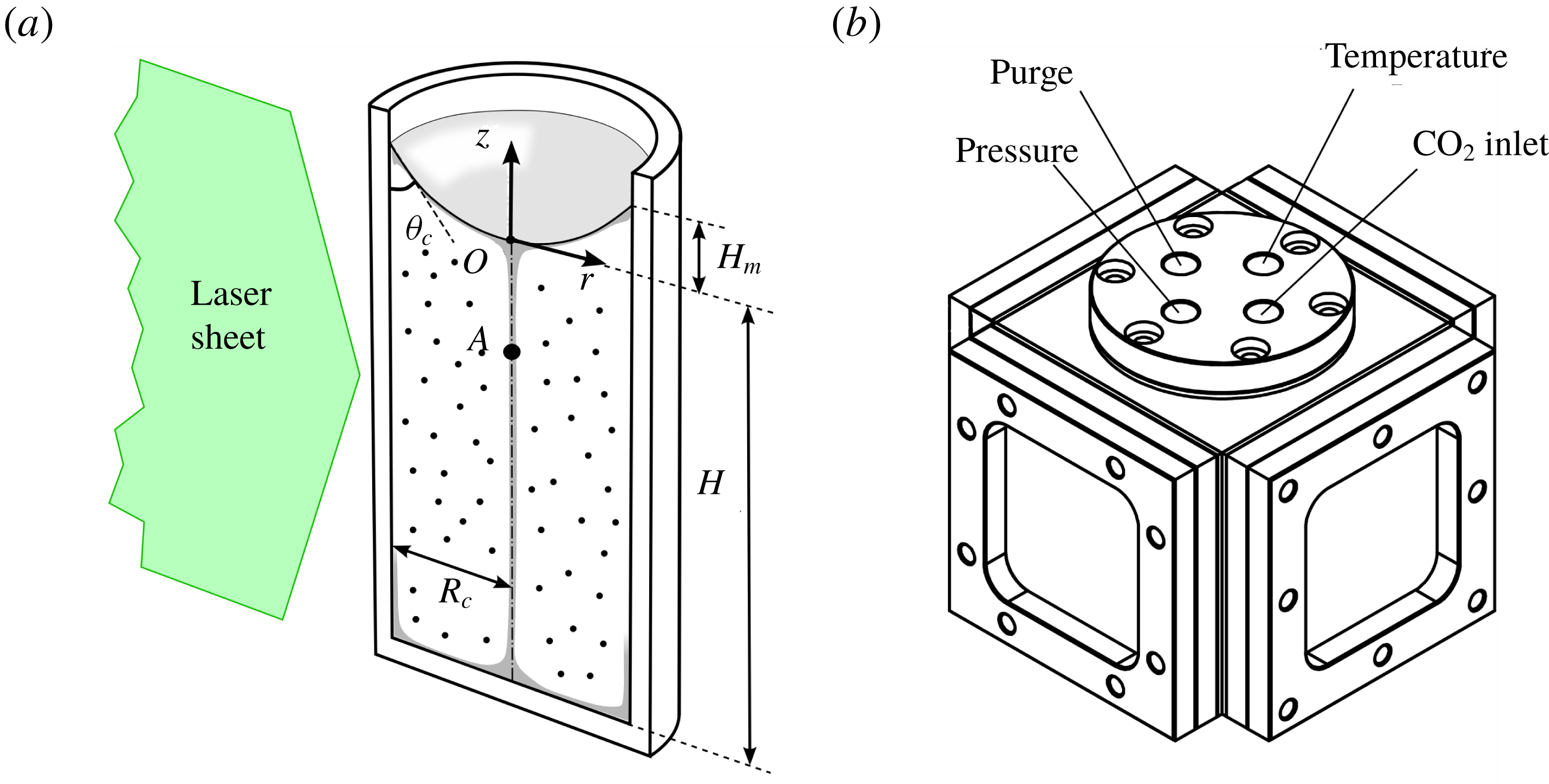
A detailed description of the experimental set-up used to characterise the flow induced in a vertical glass tube by a time step of the partial
 $\text{CO}_{2}$
pressure is given in Nadal et al. (Reference Nadal, Meunier, Pouligny and Laurichesse2013). We recall in the following the main components of the set-up. A glass cylinder of internal radius
 $R_{c}$
ranging from 4 to 8 mm and thickness 2 mm (Optik-C, France) is filled with water (density
 $\unicode[STIX]{x1D70C}_{0}$
, viscosity
 $\unicode[STIX]{x1D708}$
) up to a height
 $H$
(
 $H$
is measured from the bottom of the cylinder to the bottom of the meniscus) as shown in figure 1(a). The tube is immersed in a square optical tank full of water (not shown in figure 1), in order to reduce radial distortions of the images. There are no vertical distortions of the images because the tube is cylindrical. The whole (optical tank
 $+$
cylinder) is placed at the centre of a pressure cell (shown in figure 1
b). Four lateral sides of the pressure cell are closed by 1 cm thick quartz windows for visualisation. Flat rubber gaskets located between the quartz plates and the steel body ensure the airtightness of the cell.
Experimental set-up containing a cylindrical tube (a) filled with water and located in a pressure cell (b) filled with
 $\text{CO}_{2}$
. The fluid is seeded with particle image velocimetry (PIV) particles and the
 $\text{CO}_{2}$
enriched water creates a sinking plume (grey zone in a).

Carbon dioxide is brought into the cell by a PVC pipe (inner diameter 4 mm, outer diameter 6 mm, Legris, France) connected to the top of the pressure cell (
 $\text{CO}_{2}$
inlet in figure 1
b). The inlet jet (of the order of a few metres per second during the pressure increase) is deviated at 90 degrees toward the wall in order to prevent the forcing of disturbing motions inside the water. The 200 bar bottle (Air liquide, France) provides a 99.9 % pure carbon dioxide, the pressure of which can be adjusted using a pressure reduction valve (0–50 bars) (ref. AHL 240-16-25, Air liquide, France). For each run, the pressure is measured with a 25 bar manometer (Wika, USA) and a high precision differential 25 bar pressure sensor (Vega, Germany) connected to the top of the pressure cell (pressure in figure 1
b). Once the valve is opened, the total pressure
 $P$
rises from
 $P_{0}=1$
bar up to its final value
 $P_{1}$
in a few tens of seconds. The partial pressure of
 $\text{CO}_{2}$
increases from 0 to
 $P^{+}=P_{1}-P_{0}$
(which is directly read on the differential manometer since
 $P_{0}$
is the pressure outside the cell).
The temperature is measured using a high speed response thermocouple (TC Direct, France) located on the axis of the cylinder 4–5 mm above the meniscus through a gas-proof connection on the top of the pressure cell (temperature in figure 1
b). Both signals are recorded using a HP 34970A data logger (Hewlett Packard, USA) at a frequency of 5 Hz. During the pressurisation, the temperature rises up to 325–330 K (
 $\unicode[STIX]{x0394}T\sim 30$
K), due to the nearly adiabatic compression of the gas. This temperature increase damps over a period of 100 s. This temperature increase is larger for faster pressurisations. Although this effect could not be neglected for the study of the initial set-up of the plume (Vreme et al.
Reference Vreme, Nadal, Pouligny, Jeandet, Liger-Belair and Meunier2016), we made sure by varying the duration of the initial pressure transient that it had no effect on the characteristics of either the stationary or the unstable regimes. A fourth pipe connected to the top of the pressure cell permits purging of the system (purge in figure 1
b).
Particle image velocimetry measurements (PIV) are performed by seeding the fluid with 5
 $\unicode[STIX]{x03BC}\text{m}$
diameter polystyrene spheres (Polyscience, USA). Approximately 0.2
 $\unicode[STIX]{x03BC}\text{l}$
of the original colloidal suspension has to be diluted in 1
 $\text{cm}^{3}$
of solution, in order to obtain enough particles to perform PIV analysis. These particles are slightly denser than water, but their characteristic time of sedimentation is always much greater than the saturation time of the solution. So, these particles are considered to be good tracers. The seeded solution is periodically illuminated following a diametral plane, by a laser sheet 150
 $\unicode[STIX]{x03BC}\text{m}$
thick generated from a 670 nm red laser diode (see figure 1
b). The latter is triggered at the PIV frequency of 8 Hz by a Hewlett Packard 34970a Data Acquisition Unit (flash duration 4 ms, energy per flash 1 mJ) in order to avoid heat convection flows. The images are treated by an inter-correlation algorithm detailed in Meunier & Leweke (Reference Meunier and Leweke2003). A mask is then applied in order to remove the spurious vectors above the meniscus.
2.2 Governing equations and dimensionless numbers
Governing equations and boundary conditions will be first used to introduce the dimensionless parameters and second to present the numerical method.
Using the cylindrical coordinates, the Overbeek–Boussinesq approximation of the Navier–Stokes (NS) equations can be made dimensionless by non-dimensionalising lengths by the radius
 $R_{c}$
, times by
 $R_{c}^{2}/D$
, velocities by
 $D/R_{c}$
and pressures by
 $\unicode[STIX]{x1D70C}_{0}D^{2}/R_{c}^{2}$
(
 $D$
referring to the diffusivity of carbon dioxide in pure water). The saturation concentration at thermodynamic equilibrium
 $C^{+}=K_{H}P^{+}$
(where
 $K_{H}=3.4\times 10^{-2}~\text{mol}~\text{l}^{-1}~\text{atm}^{-1}$
denotes Henry’s constant of carbon dioxide in water) is naturally chosen as the typical concentration. Using lowercase letters for dimensionless quantities, the NS and diffusion equations can be rewritten
 $$\begin{eqnarray}\displaystyle & \displaystyle \frac{1}{S}\left[\frac{\unicode[STIX]{x2202}\boldsymbol{u}}{\unicode[STIX]{x2202}t}+(\boldsymbol{u}\boldsymbol{\cdot }\unicode[STIX]{x1D735})\boldsymbol{u}+\unicode[STIX]{x1D735}p\right]=Ra\,c\,\hat{\boldsymbol{k}}+\unicode[STIX]{x1D735}^{2}\boldsymbol{u}, & \displaystyle\end{eqnarray}$$
 $$\begin{eqnarray}\displaystyle & \displaystyle \unicode[STIX]{x1D735}\boldsymbol{\cdot }\boldsymbol{u}=0, & \displaystyle\end{eqnarray}$$
and
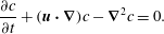 $$\begin{eqnarray}\frac{\unicode[STIX]{x2202}c}{\unicode[STIX]{x2202}t}+(\boldsymbol{u}\boldsymbol{\cdot }\unicode[STIX]{x1D735})c-\unicode[STIX]{x1D735}^{2}c=0.\end{eqnarray}$$
In equation (2.1),
 $S$
and
 $Ra$
refer to the Schmidt and solutal Rayleigh numbers, which are defined as follows
 $$\begin{eqnarray}S=\frac{\unicode[STIX]{x1D708}}{D}\quad \text{and}\quad Ra=\frac{g\unicode[STIX]{x1D6FC}K_{H}P^{+}R_{c}^{3}}{D\unicode[STIX]{x1D708}},\end{eqnarray}$$
where
 $g$
refers to the acceleration of gravity and
 $\unicode[STIX]{x1D6FC}$
refers to the chemical expansion coefficient
 $(1/\unicode[STIX]{x1D70C})(\unicode[STIX]{x2202}\unicode[STIX]{x1D70C}/\unicode[STIX]{x2202}C)$
. The experimental constants are known accurately (
 $D=1.8\times 10^{-9}~\text{m}^{2}~\text{s}^{-1}$
,
 $\unicode[STIX]{x1D708}$
varies in the range
 $[0.88;1]\times 10^{-6}~\text{m}^{2}~\text{s}^{-1}$
depending on the room temperature which was measured to within half a degree), except for the coefficient
 $\unicode[STIX]{x1D6FC}$
which is difficult to measure because the density difference is small (of the order of 0.1 %) at the concentrations considered in this paper. In the literature, the product
 $\unicode[STIX]{x1D6FC}K_{H}$
has been measured by Hebach, Oberhof & Dahmen (Reference Hebach, Oberhof and Dahmen2004) but the results of their measurements are marred by a large uncertainty (
 $\unicode[STIX]{x1D6FC}K_{H}=0.004\pm 0.001~\text{MPa}^{-1}$
), which leads to a large uncertainty (of the order of 25 %) in the experimental determination of the Rayleigh number. The density gradient due to the heat of the
 $\text{CO}_{2}$
dissolution can be neglected because it is approximately two orders of magnitude smaller than the density gradient due to the presence of
 $\text{CO}_{2}$
. Indeed, the ratio between these two density gradients is of the order of
 $(\unicode[STIX]{x1D6FC}_{H}/\unicode[STIX]{x1D6FC})(\unicode[STIX]{x0394}H_{sol}/C_{p})\sqrt{D/D_{H}}$
, where
 $\unicode[STIX]{x1D6FC}_{H}=2.07\times 10^{-4}~\text{K}^{-1}$
is the heat expansion coefficient,
 $\unicode[STIX]{x0394}H_{sol}=20500~\text{J}~\text{mol}^{-1}$
is the heat due to the
 $\text{CO}_{2}$
dissolution,
 $C_{p}=4185~\text{J}~\text{kg}^{-1}~\text{K}^{-1}$
is the specific heat capacity and
 $D_{H}=0.143\times 10^{-6}~\text{m}^{2}~\text{s}^{-1}$
is the heat diffusivity of water.
The problem must be completed by a suitable set of boundary conditions for the hydrodynamic velocity field and the gas concentration. The hydrodynamic no-slip boundary conditions at the solid walls, can be expressed as follows
 $$\begin{eqnarray}\boldsymbol{u}=\mathbf{0}\quad \text{at }\left\{\begin{array}{@{}ll@{}}r=1\quad & \text{for }z\in [-h,h_{m}]\\ z=-h\quad & \text{for }r\in [0,1],\end{array}\right.\end{eqnarray}$$
where
 $h=H/R_{c}$
and
 $h_{m}=H_{m}/R_{c}$
denote the aspect ratio of the fluid cylinder and the dimensionless depth of the meniscus respectively (see figure 1). The thermal dilatation of the water due to the absorption of
 $\text{CO}_{2}$
modifies the height of the fluid by less than 1.5 % and has been neglected. The hydrodynamic boundary condition at the meniscus is much more tricky to write. Whereas the most obvious would be to consider the vanishing of the tangential constraint at the surface (free slip), some experimental and numerical evidences tend to prove the nearly solid nature of the meniscus. Due to the contamination by surfactants and other substances, water molecules at the interface are no longer able to flow and instead behave as a solid wall (Ybert Reference Ybert1998). So, the last no-slip hydrodynamic boundary condition can be written
 $$\begin{eqnarray}\boldsymbol{u}=\mathbf{0}\quad \text{at the surface defined by }z=z_{s}(r).\end{eqnarray}$$
In the previous condition,
 $z_{s}(r)$
is the solution of the dimensionless equation (Concus Reference Concus1968)
 $$\begin{eqnarray}\frac{1}{r}\frac{\text{d}}{\text{d}r}\left[\frac{r\,\text{d}z_{s}/\text{d}r}{\sqrt{1+(\text{d}z_{s}/\text{d}r)^{2}}}\right]=Bo\,z_{s},\end{eqnarray}$$
which satisfies the condition
 $\text{d}\,z_{s}/\text{d}r=\cot \unicode[STIX]{x1D703}_{c}$
at
 $r=1$
. The contact angle
 $\unicode[STIX]{x1D703}_{c}$
of the meniscus has been measured from video images and is fairly constant in the interval
 $[25^{\circ },35^{\circ }]$
so that we took
 $\unicode[STIX]{x1D703}_{c}=30^{\circ }$
in the simulations. In (2.7), the Bond number is defined by
 $Bo=\unicode[STIX]{x1D70C}_{0}gR_{c}^{2}/\unicode[STIX]{x1D6FE}$
, where
 $\unicode[STIX]{x1D6FE}=72~\text{mN}~\text{m}^{-1}$
is the surface tension of the interface (which does not depend on the carbon dioxide concentration, see e.g. Akutsu et al.
Reference Akutsu, Yamaji, Yamaguchi, Watanabe, Smith and Inomata2007). We checked that residual gas flow (due to
 $\text{CO}_{2}$
intake) and convective flow in the liquid are not strong enough to alter the maximum interface deflection by more than 0.1 %.
Finally, one must formulate a relevant boundary condition at the surface for the gas concentration or flux. There is no reason here to consider a resistive relation between the mass flux at the interface and the deviation from the gas concentration at saturation (Cussler Reference Cussler1997). So, we make the assumption that the thermodynamic equilibrium is immediately reached at the liquid/gas interface, namely
 $$\begin{eqnarray}c=1\quad \text{at the surface defined by }z=z_{s}(r).\end{eqnarray}$$
Numerical results presented throughout the article are obtained by solving equations (2.1), (2.2) and (2.4) completed by the boundary conditions (2.5), (2.6), and (2.8) using a finite element method. The simulations are axisymmetric and the surface shape
 $z_{s}(r)$
is entered for each Bond number after solving (2.7) using Matlab. The mesh, which contains
 $2\times 10^{3}$
elements, is refined at the surface with 10 additional layers of elements having a stretching factor of 1.2. This makes the thickness of the first layer equal to 0.5 % of the tube’s radius i.e. much smaller than the thickness of the diffusive layer of
 $\text{CO}_{2}$
(of the order of 2.5 % of the radius at the largest Rayleigh number). The software uses biquadratic polynomials for the velocity, bilinear polynomials for the pressure and a bi-cubic discretisation for the
 $\text{CO}_{2}$
concentration. This leads to 200 000 degrees of freedom for an aspect ratio of 3. Simulations are initiated with
 $\boldsymbol{u}=\mathbf{0}$
,
 $c=0$
inside the fluid and are usually completed in a couple of weeks on a 64-bit PC with 2 processors at 2.4 GHz.
The Reynolds number of the plume can be defined as
 $Re=wl/S$
using the (non-dimensional) velocity
 $w$
and radius
 $l$
of the plume (
 $S$
being the Schmidt number). Using the results of Nadal et al. (Reference Nadal, Meunier, Pouligny and Laurichesse2013) for the laminar plume, the Reynolds number is found to range from 0.2 to 1.2 when the Rayleigh number ranges from
 $3\times 10^{5}$
to
 $5\times 10^{6}$
as in the experiments.
3 Instability of the steady plume
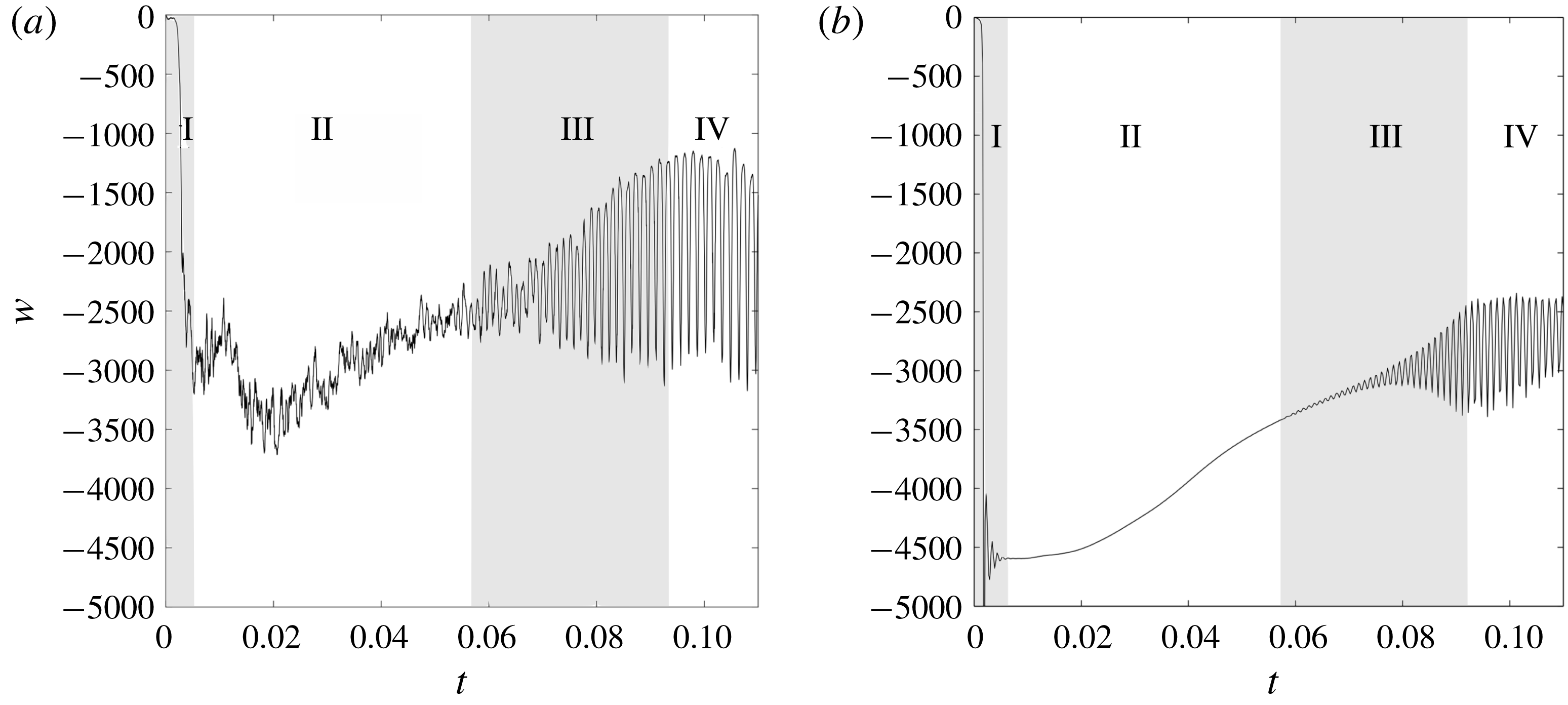
Experimental (a) and numerical (b)
 $z$
-component
 $w$
of the velocity one radius below the meniscus (
 $z=-1$
, point
 $A$
in figure 1
a) as a function of time for
 $Bo=2.2$
,
 $Ra=10^{6}$
and
 $h=4$
(
 $R_{c}=4$
mm,
 $P^{+}=6.4$
bar). Phenomenology of regimes I (transient plumes) and II (quasi-steady plume) are recalled in paragraph § 3.1. The linear instability (regime III) and its nonlinear saturation (regime IV) are detailed in paragraphs § 3.2.
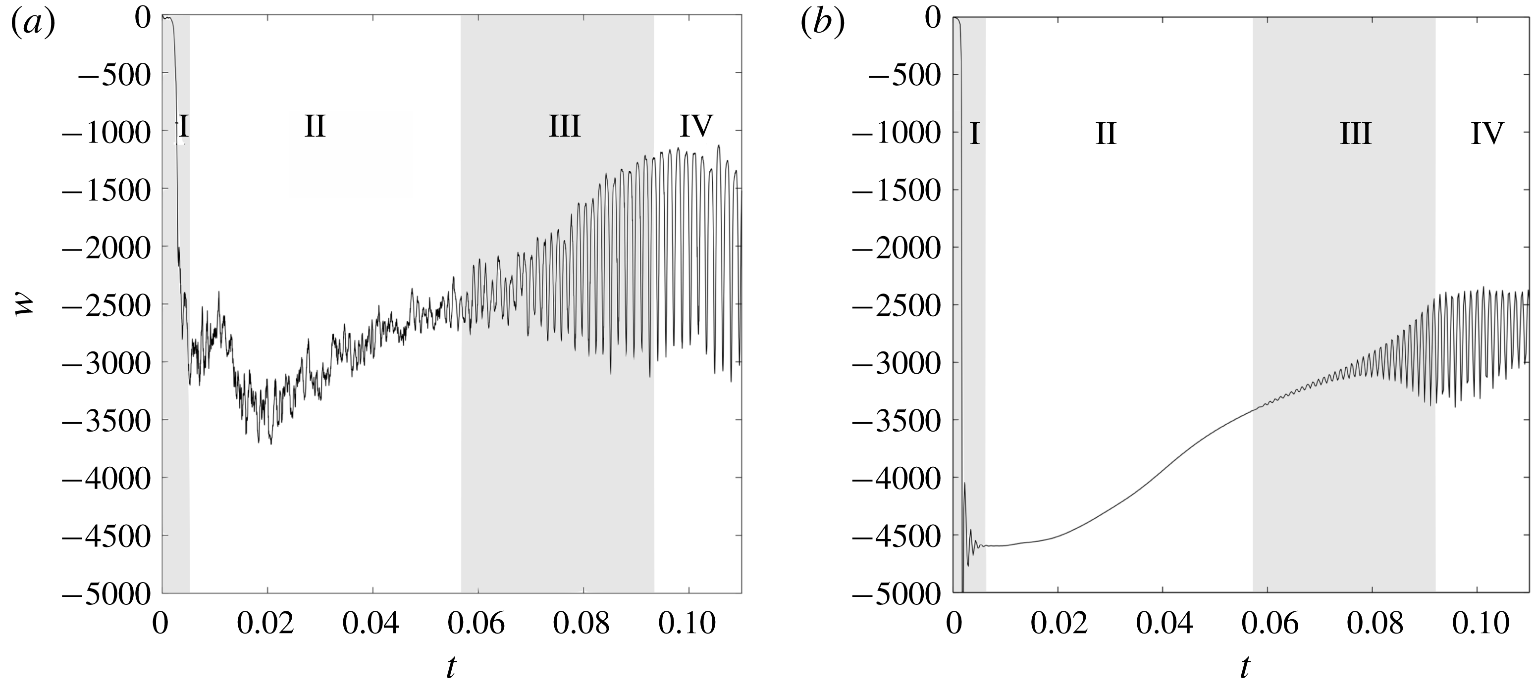
Figure 2(a,b) show generic experimental and numerical time series of the vertical component of the velocity
 $w$
as a function of time, measured one radius below the meniscus (
 $z=-1$
, point
 $A$
in figure 1). The chronology of the flow can be divided into four distinct phases, referred to as I, II, III and IV in the following. The nature of the observed phenomena and the way they are sequenced is the same for all experiments although regimes III and IV (linear and nonlinear phases of the instability) appear sooner or later depending on the dimensionless numbers of the problem (aspect ratio, Rayleigh and Bond numbers).
3.1 Regimes I and II: a quasi-steady base flow
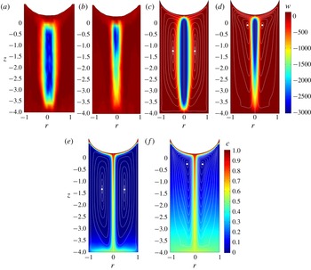
Experimental and numerical
 $z$
-component
 $w$
of the velocity at the beginning of the dissolution process (a,c
 $t=0.01$
) and just before the instability onset (b,d
 $t=0.055$
) for
 $Bo=2.2$
,
 $Ra=10^{6}$
and
 $h=4$
(
 $R_{c}=4$
mm,
 $Py^{+}=6.4$
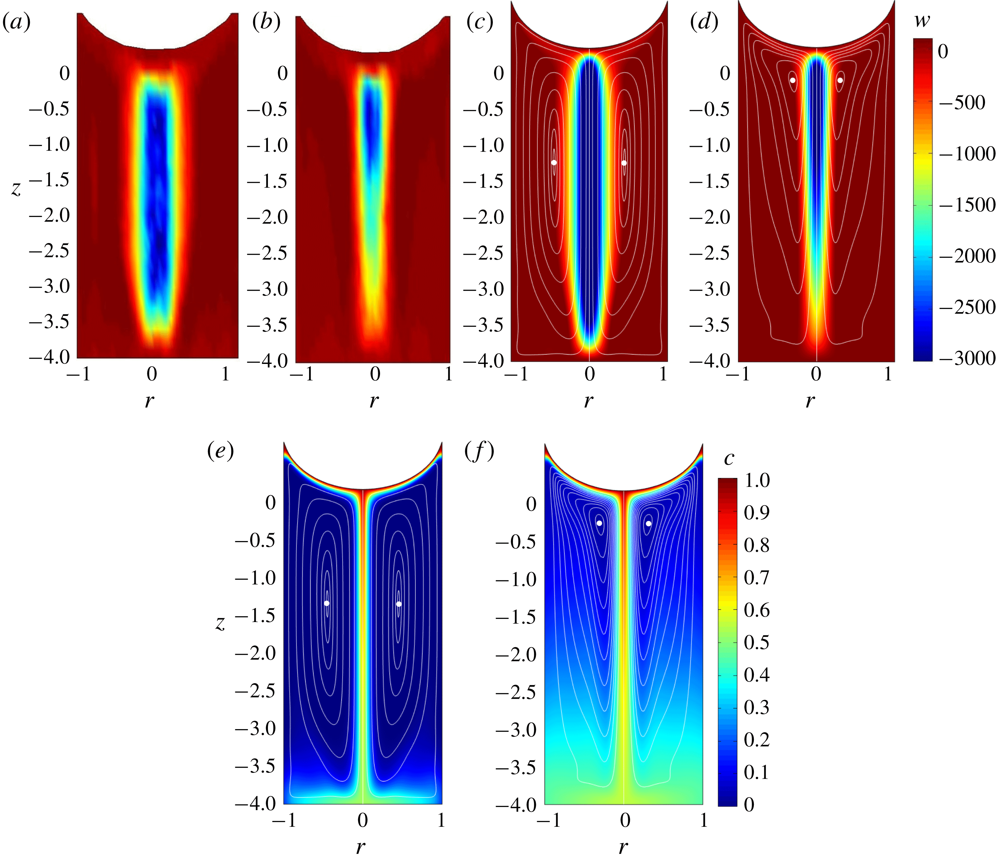
bar). Corresponding numerical concentration fields are shown on (e) and (f). Streamlines (white solid lines) are superimposed to numerical fields. White dots show the position of the elliptic stagnation points.
Once the inlet is open (
 $t=0$
), the carbon dioxide creates a diffusive gas enriched layer of dense fluid beneath the surface, which is unstable from a gravitational point of view. A plume is formed, which propagates downwards to the bottom of the cell. This transient plume is followed by a few others (typically 3 or 4) at a frequency of about 1 Hz, which corresponds to approximately 1000 in non-dimensional frequency units. This first transient regime (I) is very short (of the order of 0.003 dimensionless time units). After this period of time, the rapid oscillations of the velocity disappear completely in the numerical simulations and remain weak in the experiments. A nearly stationary regime (II) settles in the tube. The velocity of the plume slowly decreases by 25 % during stage II. It can be noted that the velocity amplitude is 20 % smaller in the experiments than in the numerical simulations. This could be due to small oscillations and asymmetries on the base flow in the experiment (especially visible at large Bond numbers).
At the beginning of stage II, the plume is composed of a stem with parallel streamlines. The stem fills the whole height of the cylinder (see experimental and numerical velocity shown in figure 3
a,c) and the amplitude of the velocity is independent of
 $z$
along the axis from
 $z=-0.5$
to
 $z=-3.5$
. By contrast, figure 3(b,d) shows that at the end of stage II the vertical velocity is smaller at the bottom of the plume (around
 $z=-3$
) than at the top (around
 $z=-1$
). This is due to the gradual filling of the tube by the saturated solution which reduces the concentration difference between the plume and the surrounding medium. For example, the density fields obtained numerically (figure 3
e,f) indicate that the difference in concentration
 $c$
between the axis and the outer part of the plume (at the bottom of the cylinder) is roughly equal to 0.6 at the beginning of stage II and to 0.3 at the end of stage II. This filling-box effect decreases the velocity of the plume at the bottom of the tube, and has an overall effect on the streamlines. The ‘rotation centre’, (i.e. the elliptic stagnation point highlighted by a white dot in figure 3
c–f) is located at
 $z=-1.5$
at the beginning of stage II. It gets closer to the free surface as time evolves and reaches the altitude
 $z=-0.5$
at the end of stage II. After a long period of time, the amplitude of the oscillations resumes growing (stage III), indicating that the slowly evolving plume has become suddenly unstable. The nearly stationary plume is considered as the base flow of the instability depicted in the following.
3.2 Regimes III and IV: a sudden destabilisation of the flow
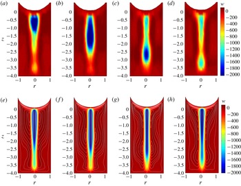
(a–d) Experimental and numerical (e–h)
 $z$
-component of velocity at
 $t=0.1$
(a,e),
 $t=0.1+\unicode[STIX]{x1D70F}_{NL}/4$
(b,f),
 $t=0.1+\unicode[STIX]{x1D70F}_{NL}/2$
(c,g),
 $t=0.1+3\,\unicode[STIX]{x1D70F}_{NL}/4$
(d,h), where
 $\unicode[STIX]{x1D70F}_{NL}=0.0015$
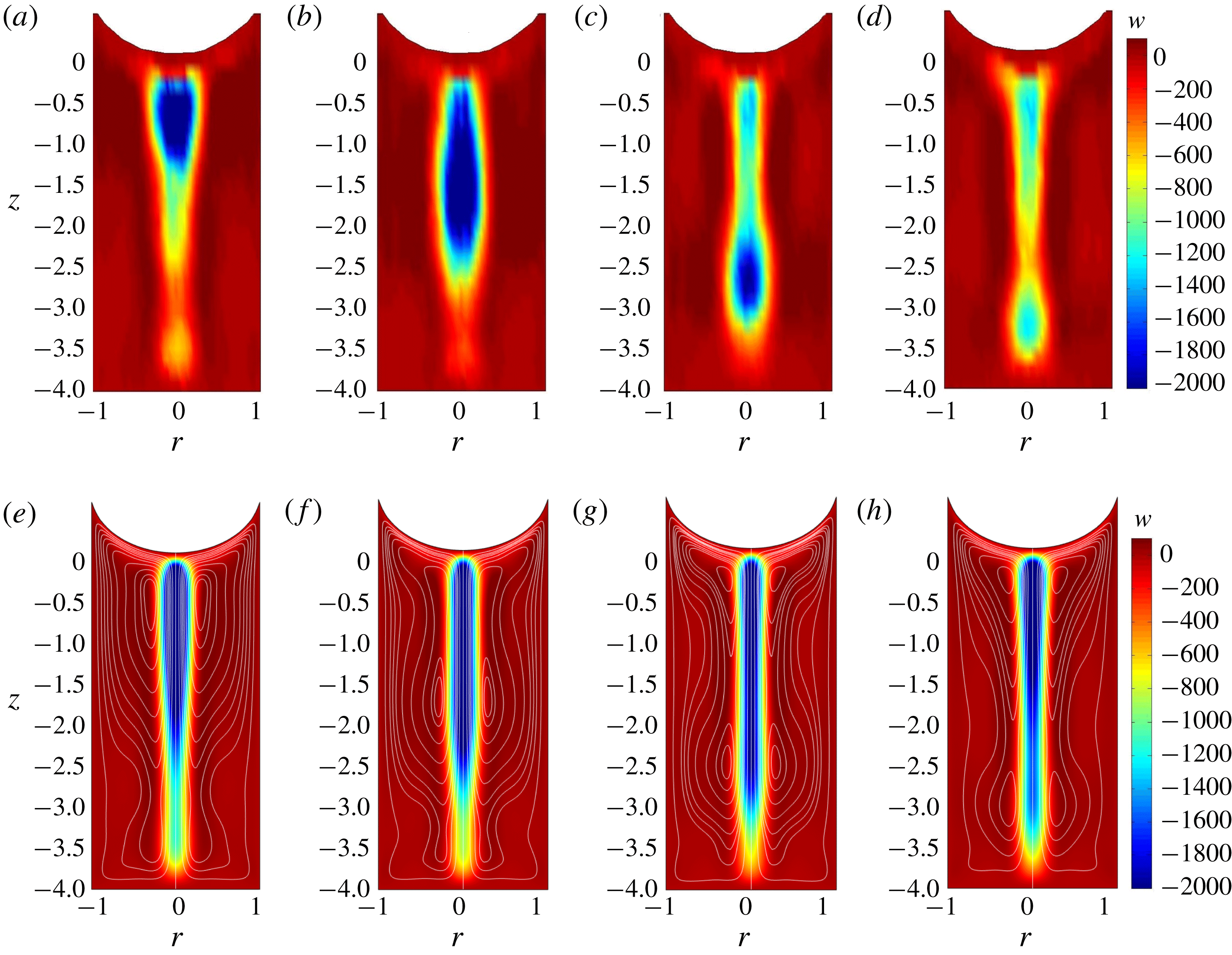
is the period of the instability in the nonlinear regime.
 $Ra=10^{6}$
,
 $h=4$
,
 $Bo=2.2$
.
After a long period of time
 $t_{i}$
, the vertical velocity of the plume is subject to rapidly growing oscillations which characterise the linear instability (regime III). The onset time seems to correspond to the instant when the altitude of the rotation centre is close to
 $z=-1$
. The velocity oscillations correspond to an axisymmetric varicose mode in which broadenings are advected down to the bottom of the cell (regime III, see supplementary materials movie1.avi, available at https://doi.org/10.1017/jfm.2018.564). In the first oscillatory regime (period
 $\unicode[STIX]{x1D70F}$
, frequency
 $\unicode[STIX]{x1D71B}=2\unicode[STIX]{x03C0}/\unicode[STIX]{x1D70F}$
) the velocity amplitude grows rapidly during few tens of periods (10 to 20 typically). The amplitude of the oscillations then saturates and the period of the instability switches to a slightly larger value
 $\unicode[STIX]{x1D70F}_{NL}>\unicode[STIX]{x1D70F}$
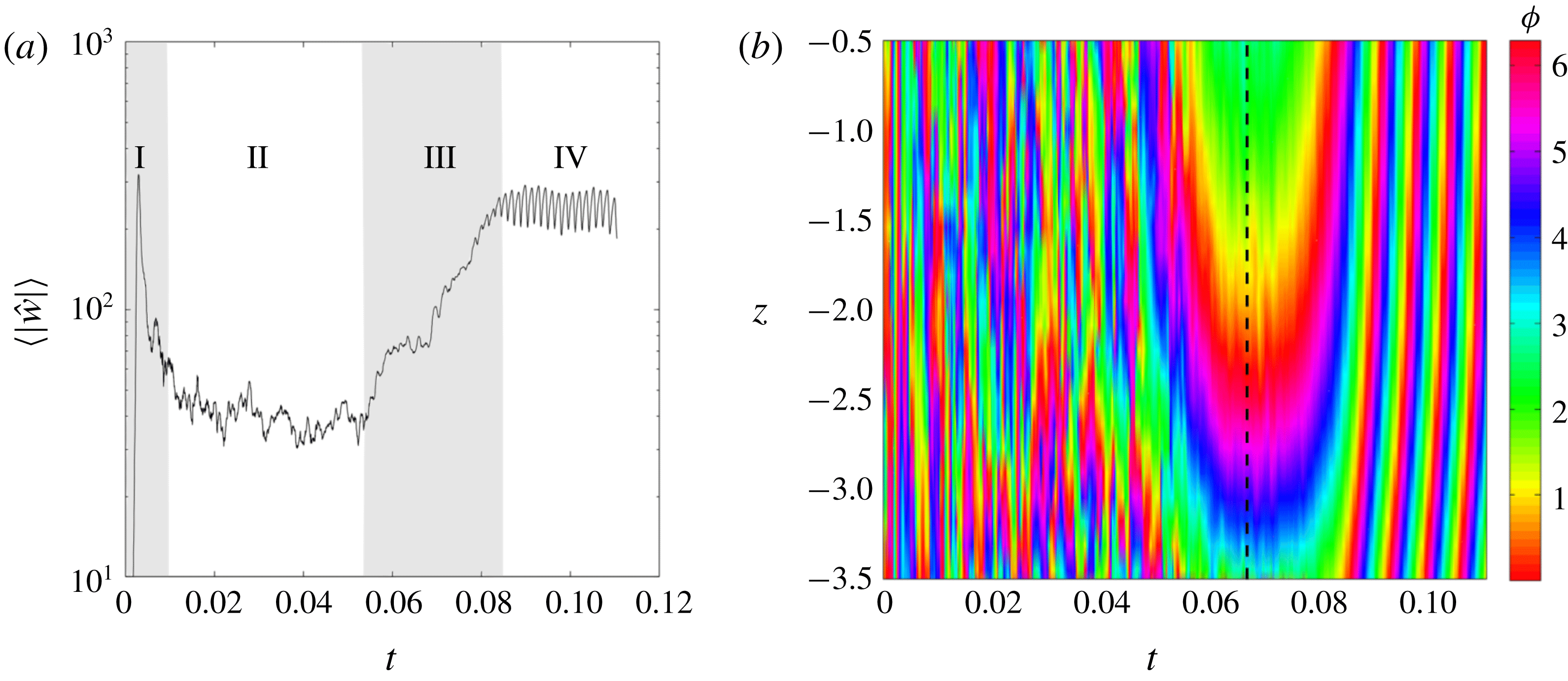
. In the latter nonlinear regime (IV), the broadenings of the varicose instability evolve towards dissociated blobs which periodically pour from the meniscus, as shown in figure 4(a–d). The puffs are less visible in the numerical simulations (figure 4
e–h) since the instability saturates at a lower amplitude (possibly due to numerical diffusion). Then, the period of the nonlinear regime slowly keeps increasing in time. In some rare experimental cases a second frequency steps in, leading to a quasi-periodic flow. The next paragraphs are devoted to a quantitative description of the instability (regimes III and IV).
3.3 Frequency of the perturbation
(a) Time evolution of the amplitude of
 ${\hat{w}}$
averaged in the domain
 $[|r|<0.15,-3.5<z<-0.5]$
. (b) Spatio-temporal diagram of the argument of the
 $\unicode[STIX]{x1D71B}_{0}$
-transform (3.1), averaged for
 $|r|<0.15$
. Here
 $Bo=2.2$
,
 $Ra=10^{6}$
and
 $h=4$
.
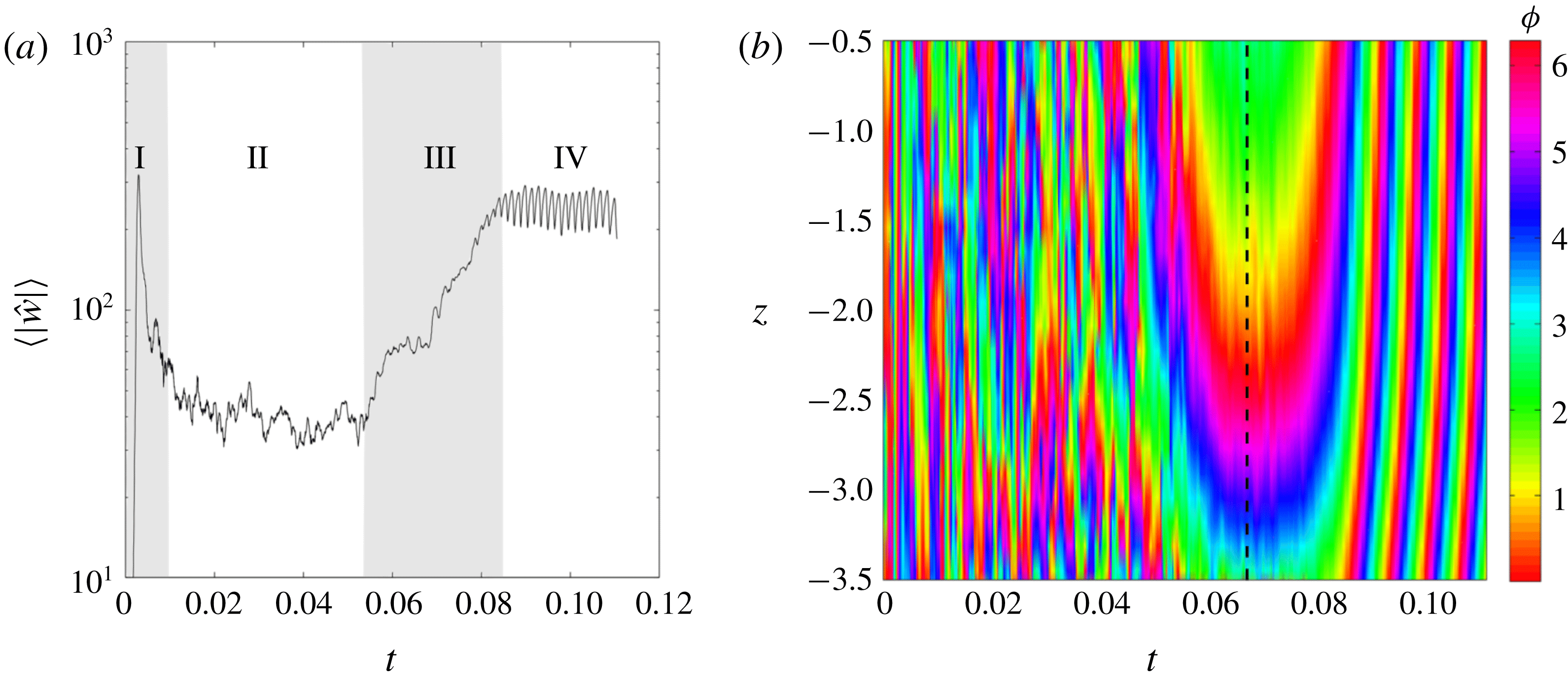
To determine the characteristics of the instability accurately, the perturbation is separated from the base flow by taking the temporal Fourier transform of the vertical velocity over a sliding window. The vertical velocity
 $w(r,z,t)$
obtained from PIV measurements is first multiplied by
 $\exp \text{i}\unicode[STIX]{x1D71B}_{0}t$
, where
 $\unicode[STIX]{x1D71B}_{0}$
is iteratively adjusted for each experiment to get as close as possible to the experimental frequency
 $\unicode[STIX]{x1D71B}$
, then averaged over a period
 $\unicode[STIX]{x1D70F}_{0}=2\unicode[STIX]{x03C0}/\unicode[STIX]{x1D71B}_{0}$
leading to a complex velocity
 ${\hat{w}}(r,z)$
. The integration over a period
 $\unicode[STIX]{x1D70F}_{0}$
allows us to eliminate the stationary component of the flow. At the same time, if we assume that the vertical component of the perturbation is of the form
 $\bar{w}(r)\,\exp \text{i}(kz-\unicode[STIX]{x1D71B}t)+\text{c.c.}$
(where
 $\text{c.c.}$
corresponds to the complex conjugate) the previous operation provides the spatial structure of the perturbation since
 $$\begin{eqnarray}{\hat{w}}(r,z)=\frac{1}{\unicode[STIX]{x1D70F}_{0}}\int _{t}^{t+\unicode[STIX]{x1D70F}_{0}}\bar{w}(r)\,\text{e}^{\text{i}(kz-\unicode[STIX]{x1D71B}t^{\prime })}\text{e}^{\text{i}\unicode[STIX]{x1D71B}_{0}t^{\prime }}\,\text{d}t^{\prime }=\bar{w}(r)\,\text{e}^{\text{i}kz}\quad \text{for }\unicode[STIX]{x1D71B}_{0}=\unicode[STIX]{x1D71B}.\end{eqnarray}$$
The amplitude
 $|{\hat{w}}|$
of the perturbation is displayed in figure 5(a). In the stable regime (stage II), the amplitude of the
 $\unicode[STIX]{x1D71B}_{0}$
-Fourier component remains weak and stationary; this is due to the noise in the measurements. At the end of the stable regime, the amplitude of the
 $\unicode[STIX]{x1D71B}_{0}$
-Fourier component grows by approximately one order of magnitude (stage III). The amplitude then saturates when the system enters the nonlinear regime IV.
Clearly, this process relies on the choice of the Fourier frequency
 $\unicode[STIX]{x1D71B}_{0}$
which is tuned once for each experiment in order to get stationary iso-phases during the linear stage. Figure 5(b) shows the temporal evolution of the phase
 $\unicode[STIX]{x1D719}=\text{arg}({\hat{w}})$
of the
 $\unicode[STIX]{x1D71B}_{0}$
-Fourier component on the axis of the plume. Before
 $t=0.06$
, the instability is too weak such that the argument has no physical meaning (noise). Between
 $t=0.06$
and
 $t=0.085$
, the iso-phases are nearly stationary for the Fourier frequency
 $\unicode[STIX]{x1D71B}_{0}$
has been chosen as close as possible to the frequency
 $\unicode[STIX]{x1D71B}$
of the instability. After
 $t=0.08$
, the iso-phases of the
 $\unicode[STIX]{x1D71B}_{0}$
-Fourier component are no longer stationary: they are translated in the positive
 $z$
-direction since the period of the oscillations in the nonlinear regime is slightly larger than in the linear regime (by approximately 20 %). The error on
 $\unicode[STIX]{x1D71B}$
is of the order of 5 to 10 % since the linear stage only lasts for 10 to 20 periods. It should be noted that the determination of the frequency is deduced from velocity measurements along the whole axis.
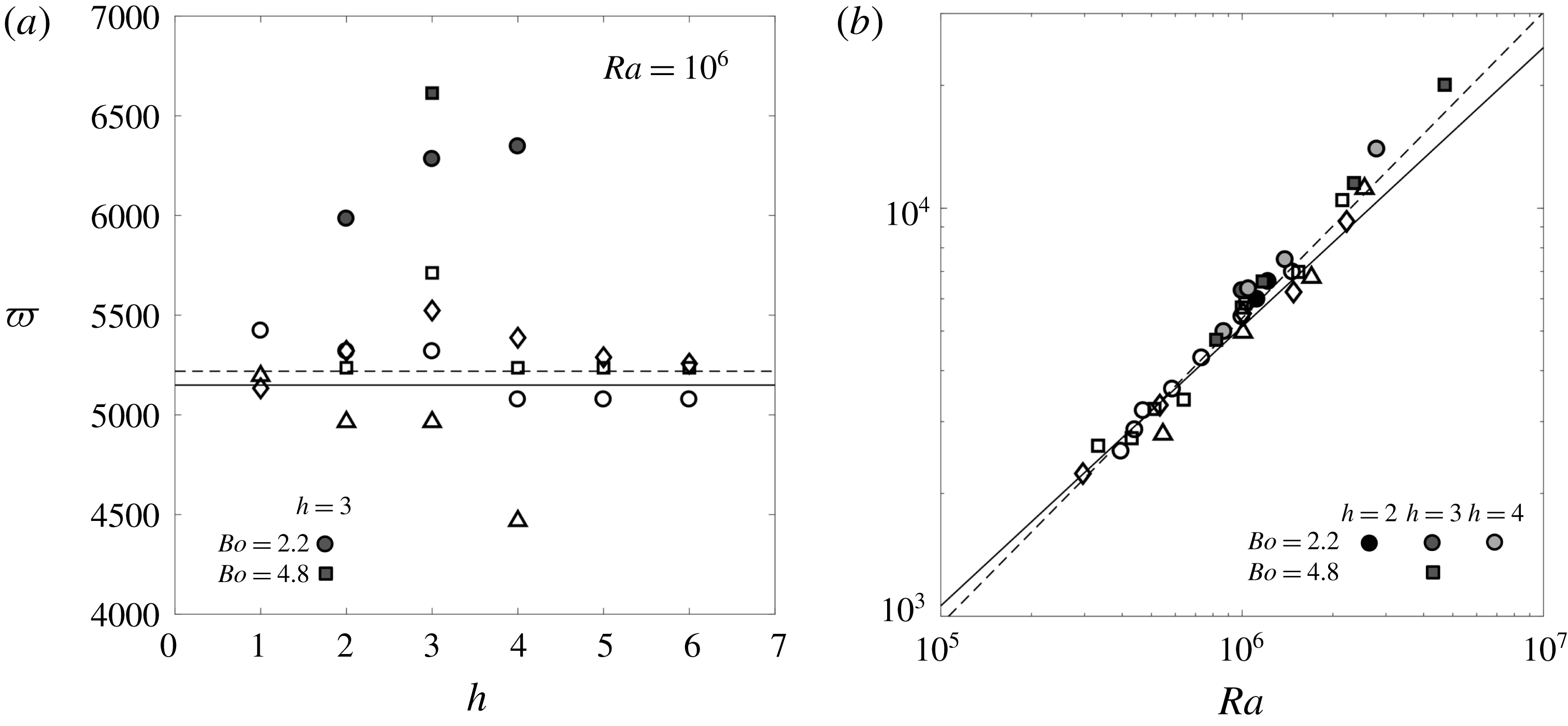
The frequency of the instability in the linear regime is plotted in figure 6 as a function of the aspect ratio (a) and Rayleigh number (b). Figure 6 shows that the experimental data are practically independent of the Bond number. The frequency obtained in this configuration (with a meniscus) can thus be extrapolated to flat free surfaces (without meniscus) which correspond to infinite Bond numbers. Figure 6(a) also indicates that the frequency is independent of the aspect ratio within the experimental range. Finally, figure 6(b) reveals that the frequency strongly depends on the Rayleigh number. It can be fitted by the power law
 $$\begin{eqnarray}\unicode[STIX]{x1D71B}=0.165\,Ra^{3/4},\end{eqnarray}$$
with a small uncertainty in the measurements. Numerical results overestimate the experimental values by approximately
 $20\,\%$
, but are still consistent in order of magnitude (the overestimate is less visible in figure 6(b) due to the logarithmic scale of the vertical axis).
Frequency of the instability (linear growth) as a function of (a) the aspect ratio
 $h$
and (b) the Rayleigh number
 $Ra$
. The Bond number is equal to 2.2 (circles,
 $R_{c}=4$
mm), 3.4 (diamonds,
 $R_{c}=5$
mm), 4.8 (squares,
 $R_{c}=6$
mm) and 8.6 (triangles,
 $R_{c}=8$
mm). Experimental results (open symbols) are compared to the numerical results (solid symbols). The dashed line is the best power fit (3.2) of the experimental data. The theoretical prediction (solid line) corresponds to the fluid velocity in a stationary plume (
 $w_{\unicode[STIX]{x1D719}}=0.17\,Ra^{2/3}(\log Ra)^{1/3}$
) times a constant empirical value of the wavenumber
 $k=1.5$
(see equation (3.6)). The error in the experimental determination of
 $\unicode[STIX]{x1D71B}$
is smaller than 10 %.

3.4 Wavenumber and phase velocity of the perturbation
In order to obtain the wavenumber of the perturbation, the phase
 $\unicode[STIX]{x1D719}=\text{arg}({\hat{w}})$
is fitted by a linear function
 $\unicode[STIX]{x1D719}=kz$
during stage III when
 $\unicode[STIX]{x1D719}$
is stationary in time (i.e. around
 $t=0.067$
in figure 5
a). Indeed, if the frequency
 $\unicode[STIX]{x1D71B}_{0}$
is equal to the frequency
 $\unicode[STIX]{x1D71B}$
of the mode, equation (3.1) indicates that
 $k$
is the wavenumber of the perturbation.
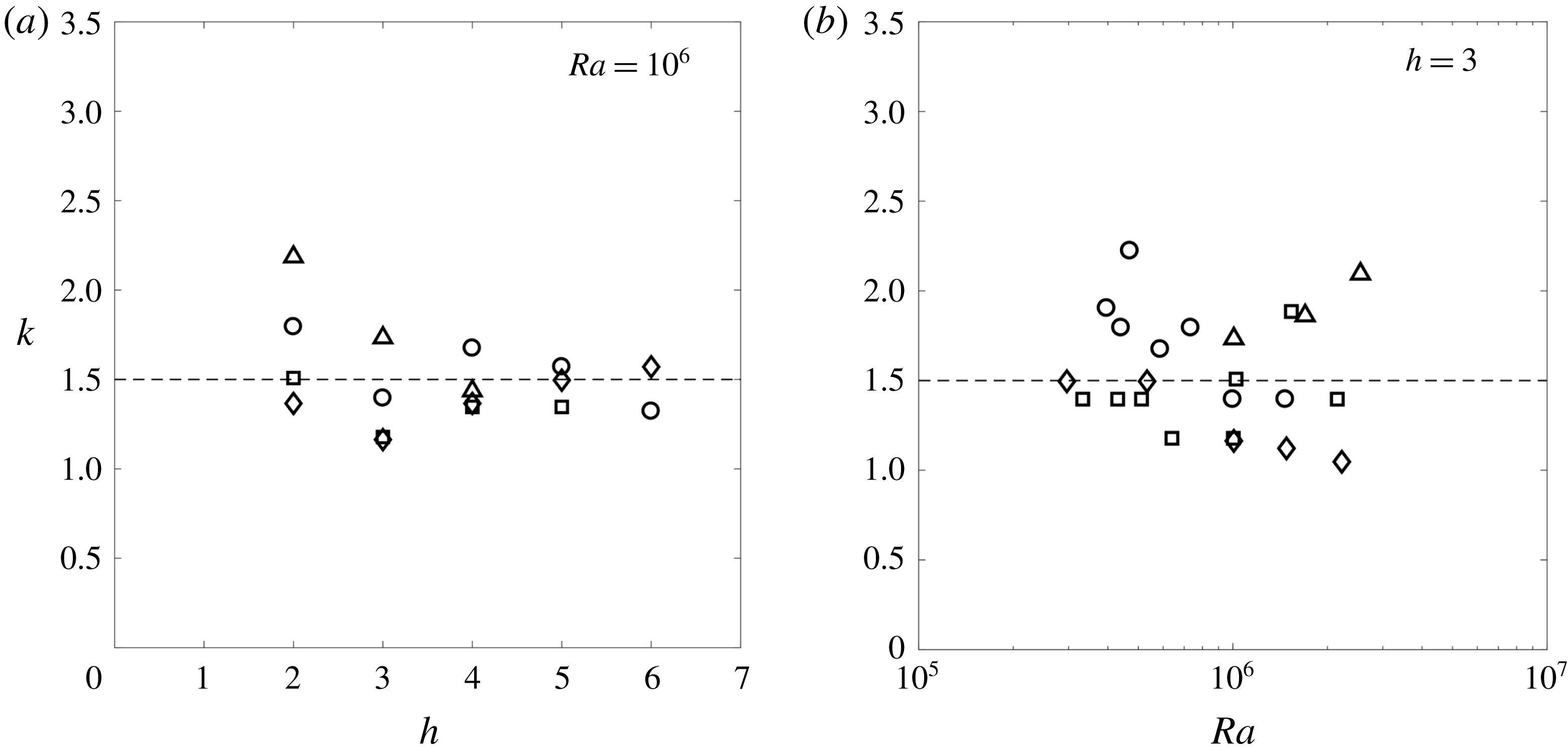
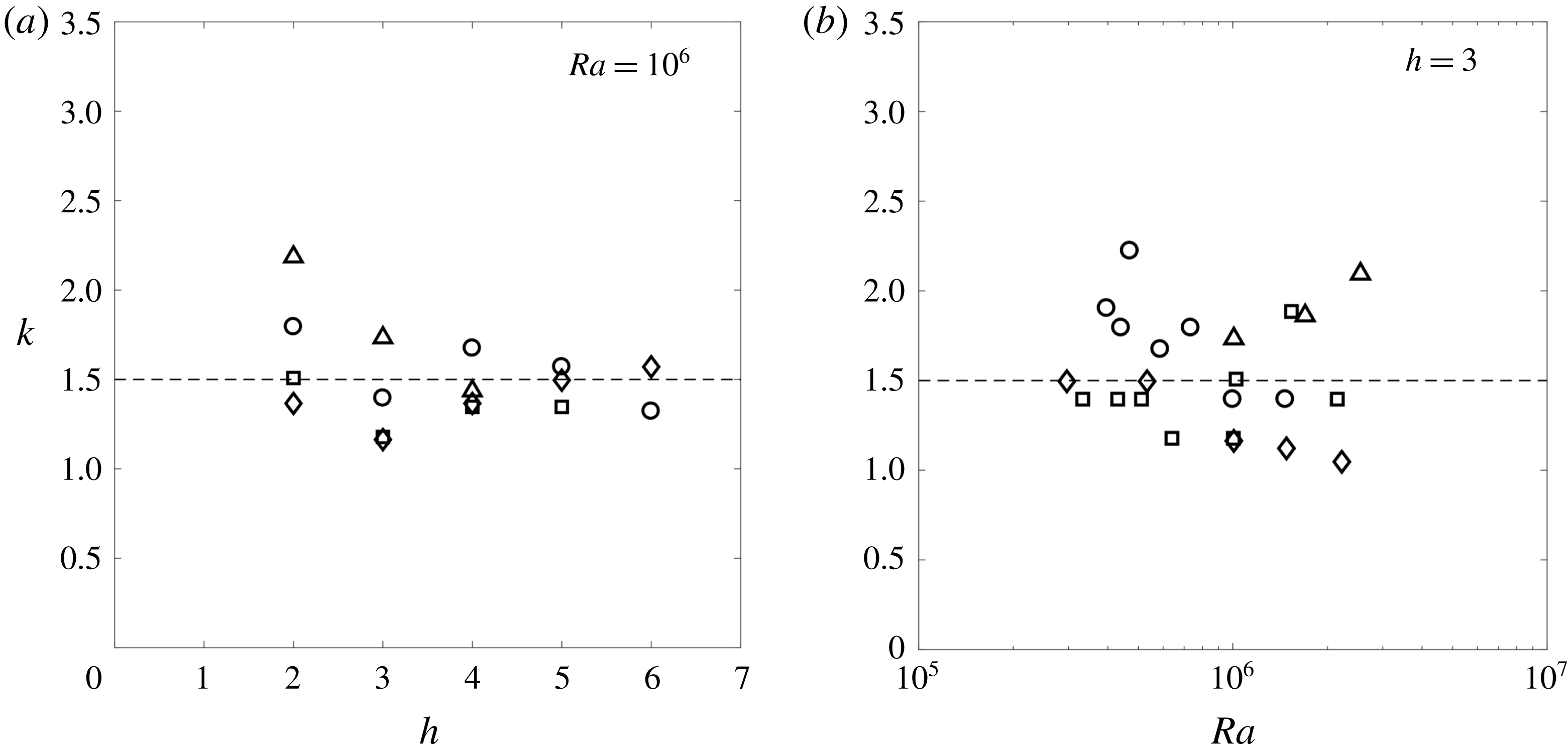
The wavenumber is plotted as a function of the Rayleigh number for
 $h=3$
in figure 7(a), and as a function of the aspect ratio for
 $Ra=10^{6}$
in figure 7(b). Due to the noise in the measurements of the vertical velocity, the evaluation of the wavenumber is marred by a large uncertainty (
 ${\sim}45\,\%$
). However, the mean wavenumber (averaged over the Rayleigh number and the aspect ratio) does not vary by more than 15 % when the Bond number increases from 2 to 9. This tends to indicate that these results may be extrapolated to the cases of flat free surfaces. More surprisingly, no clear dependence on the Rayleigh number or aspect ratio can be identified. Consequently, the experimental wavenumber is considered as independent of any dimensionless number. The value
 $$\begin{eqnarray}k=1.5\end{eqnarray}$$
(in non-dimensional form), which corresponds to the best fitting value of the experimental data, is plotted as dashed lines in figure 7(a,b).
Wavenumber of the instability as a function of (a) the aspect ratio, for
 $Ra=10^{6}$
and (b) the Rayleigh number for
 $h=3$
. The Bond number is equal to
 $Bo=2.2$
(circles),
 $Bo=3.4$
(diamonds),
 $Bo=4.8$
(squares) and
 $Bo=8.6$
(triangles). The dashed line corresponds to the best fitting value given by (3.3). The error in the experimental determination of
 $k$
ranges from 20 to 30 %.
It has also been observed that the phase
 $\unicode[STIX]{x1D719}$
was not always linear in
 $z$
:
 $\unicode[STIX]{x1D719}$
may increase faster at the bottom than at the top. This means that the wavenumber is larger at the bottom than at the top. The values reported here correspond to the mean value of the wavenumber (evaluated between
 $z=1-h$
and
 $z=-1$
in order to remove the noisy PIV measurements at the top and the bottom).
The phase velocity of the instability, which can be deduced from the frequency and wavenumber of the instability via the relationship
 $w_{\unicode[STIX]{x1D719}}=\unicode[STIX]{x1D71B}/k$
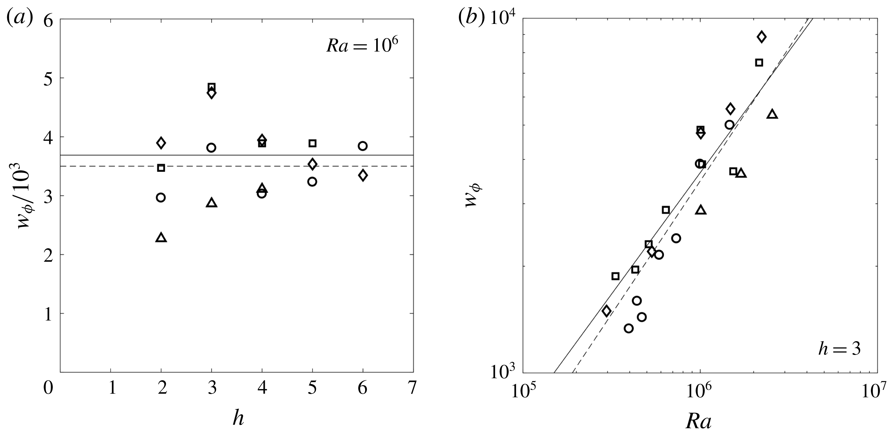
, is plotted in figure 8. As observed for the frequency and the wavenumber, the experimental phase velocity of the instability is independent of the Bond number. As deduced from the measurements on
 $\unicode[STIX]{x1D71B}$
and
 $k$
, no clear dependence of the phase velocity
 $w_{\unicode[STIX]{x1D719}}$
on the aspect ratio can be identified (see figure 8
a), at least in the limit of the measurement uncertainty (due to the large dispersion observed on
 $k$
).
Phase velocity of the instability as a function of (a) the aspect ration
 $h$
and (b) the Rayleigh number
 $Ra$
. The Bond number is equal to 2.2 (circles), 3.4 (diamonds), 4.8 (squares) and 8.6 (triangles). Experimental results (open symbols) and numerical results (filled symbols) are fitted (dashed line) by a power law (3.4). The solid line corresponds to the theoretical prediction (3.5) of the fluid velocity for a stationary plume given in Nadal et al. (Reference Nadal, Meunier, Pouligny and Laurichesse2013). The error is of the order of 30 %.
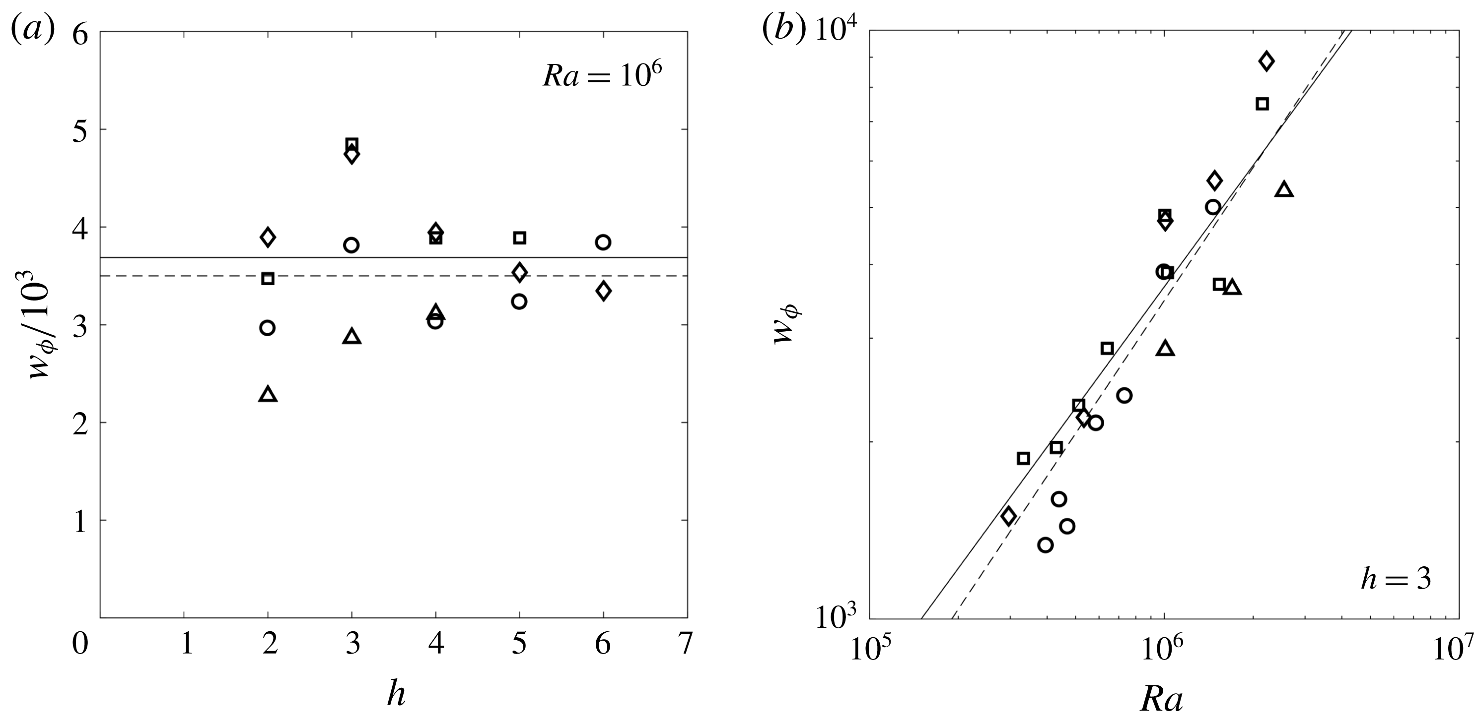
As obtained for the frequency, the phase velocity strongly depends on the Rayleigh number. It can be fitted by the power law
 $$\begin{eqnarray}w_{\unicode[STIX]{x1D719}}=0.11\,Ra^{3/4}\end{eqnarray}$$
in agreement with the relation
 $w_{\unicode[STIX]{x1D719}}=\unicode[STIX]{x1D71B}/k$
. It can be noted that the phase velocity of the instability is close to the fluid velocity of the plume itself. Nadal et al. (Reference Nadal, Meunier, Pouligny and Laurichesse2013) found theoretically, experimentally and numerically that the laminar steady plume (stage II) has a velocity given by the intrinsic (parameter free) modified power law
 $$\begin{eqnarray}w=0.17\,Ra^{2/3}(\log Ra)^{1/3},\end{eqnarray}$$
where the constant 0.17 was obtained from Nadal et al. (Reference Nadal, Meunier, Pouligny and Laurichesse2013). This expression of the plume velocity is plotted as a solid line in figure 8. It is very close to the experimental results for the phase velocity of the instability (despite the absence of adjustable parameters). This means that the instability is mostly advected by the base flow in the linear regime and does not propagate relative to the fluid. This result will be a key point in the qualitative model presented in § 4 and appendix A.
It can be noted that the local phase velocity is actually smaller at the bottom than at the top (because the wavenumber is larger at the bottom than at the top). This is again in agreement with the assumption that the perturbation is advected at the fluid velocity of the plume. Indeed, the vertical velocity of the plume is smaller at the bottom than at the top due to the background stratification (as stated in § 3.1).
Finally, using the relation
 $w_{\unicode[STIX]{x1D719}}=\unicode[STIX]{x1D71B}/k$
, the theoretical value of the plume velocity (3.5) and the empirical value of the wavenumber
 $k=1.5$
, the frequency of the plume can be given semi-theoretically as
 $$\begin{eqnarray}\unicode[STIX]{x1D71B}=0.255\,Ra^{2/3}(\log Ra)^{1/3}.\end{eqnarray}$$
This prediction plotted in solid lines in figure 6 is again fairly close to the experimental and numerical values.
3.5 Onset time
In every experimental run, the instability appeared at a fairly reproducible time
 $t_{i}$
strongly depending on the aspect ratio and Rayleigh number (the experiments have been repeated four times at
 $Ra=10^{6}$
,
 $h=3$
and
 $Bo=4.8$
). Furthermore, contrary to what is observed for other quantities (frequency, wavenumber, phase velocity), the onset time does depend on the Bond number: the plume destabilises later for smaller Bond numbers, indicating that the meniscus has a stabilising effect. Such an effect can be intuitively understood as follows. The slope of the meniscus induces solutal baroclinicity underneath the free surface which tends to force the heavy fluid towards the axis. The baroclinic
 $\text{CO}_{2}$
enriched fluid located underneath the interface near the contact line is advected fast enough towards the bottom of the meniscus to prevent the growth of any fingering instability (other than the main central plume).
Since the Bond number characterises the degree of flatness of the meniscus, this effect is expected to saturate at large Bond numbers, where the radius of the cylinder is larger than the capillary length
 $l_{c}=(\unicode[STIX]{x1D6FE}/\unicode[STIX]{x1D70C}_{0}g)^{1/2}$
. In an attempt to make all the results collapse onto a single curve, the onset time
 $t_{i}$
has been rescaled by a function
 $f(Bo)=(1+Bo^{-1})^{\unicode[STIX]{x1D6FD}}$
which tends to 1 in the limit of large Bond numbers. The rescaled onset time
 $\tilde{t}_{i}=f(Bo)\,t_{i}$
is plotted in figure 9 with an exponent
 $\unicode[STIX]{x1D6FD}$
adjusted to
 $-3.5$
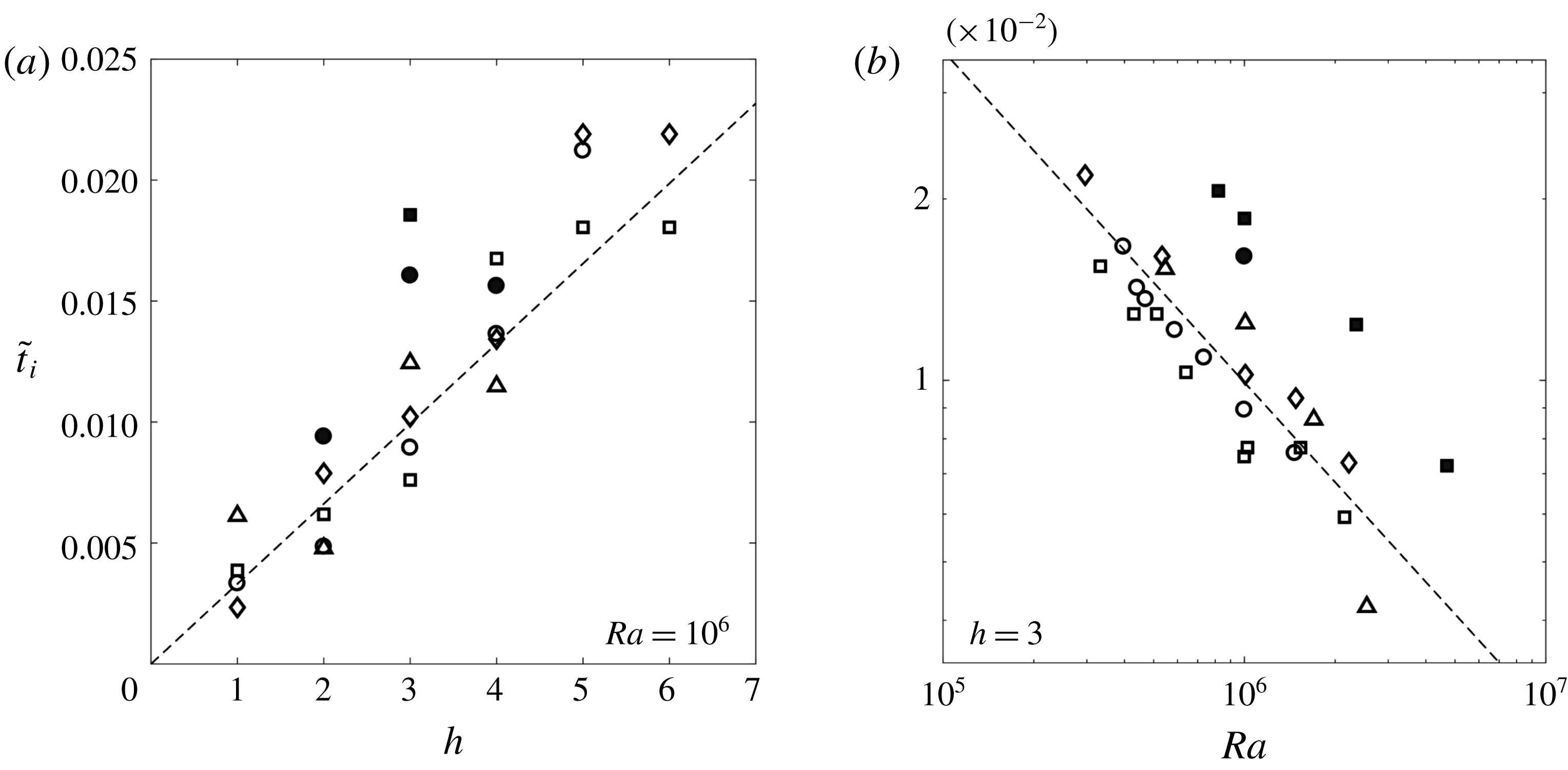
. Figure 9(a) shows that the rescaled onset time
 $\tilde{t}_{i}$
is proportional to the height of the cylinder, at fixed Rayleigh number. As mentioned at the beginning of paragraph § 3.2, the destabilisation seems to occur as soon as the streamlines are confined to a region of vertical extent unity (
 $R_{c}$
in dimensional terms) or equivalently, when the ‘rotation centre’ of the streamlines is located around
 $z=-1$
. So, considering that the flow becomes unstable once the background stratification has filled the cylinder up to a specific height and recalling that the dimensionless buoyancy flux
 $Sh$
(Sherwood number) of a steady laminar plume scales as
 $Sh\sim Ra^{1/3}$
(see Nadal et al.
Reference Nadal, Meunier, Pouligny and Laurichesse2013) leads to a scaling of the form
 $\tilde{t}_{i}\sim \,h\,Ra^{-1/3}$
. Such an interpretation is consistent with the scenario proposed in § 4, where the instability is triggered by what is called a ‘filling-box’ effect by Lopez & Marques (Reference Lopez and Marques2013). The linear scaling between the onset time and the height of the cylinder is well recovered experimentally, as shown in figure 9(a).
Rescaled onset time of the instability
 $\tilde{t}_{i}=(1+Bo^{-1})^{-3.5}\,t_{i}$
as a function of (a) the aspect ratio
 $h$
and (b) the Rayleigh number
 $Ra$
. The Bond number is equal to 2.2 (circles), 3.4 (diamonds), 4.8 (squares) and 8.6 (triangles). Dashed lines correspond the best fit of the experimental data by the power law (3.7). Experimental and numerical data are plotted with open and solid symbol respectively. The error in the experimental determination of
 $t_{i}$
is of the order of 20 %.

That being said, the real flow and stratification are not that simple and the above explanation is only an idealised view of the problem. The scaling on the Rayleigh number is thus slightly different in the experiments. Figure 9(b) shows that the decrease of the rescaled onset time with the Rayleigh number can be roughly rendered by a power fitting law
 $$\begin{eqnarray}\tilde{t}_{i}=6.61\,h\,Ra^{-0.55},\end{eqnarray}$$
as shown in figure 9.
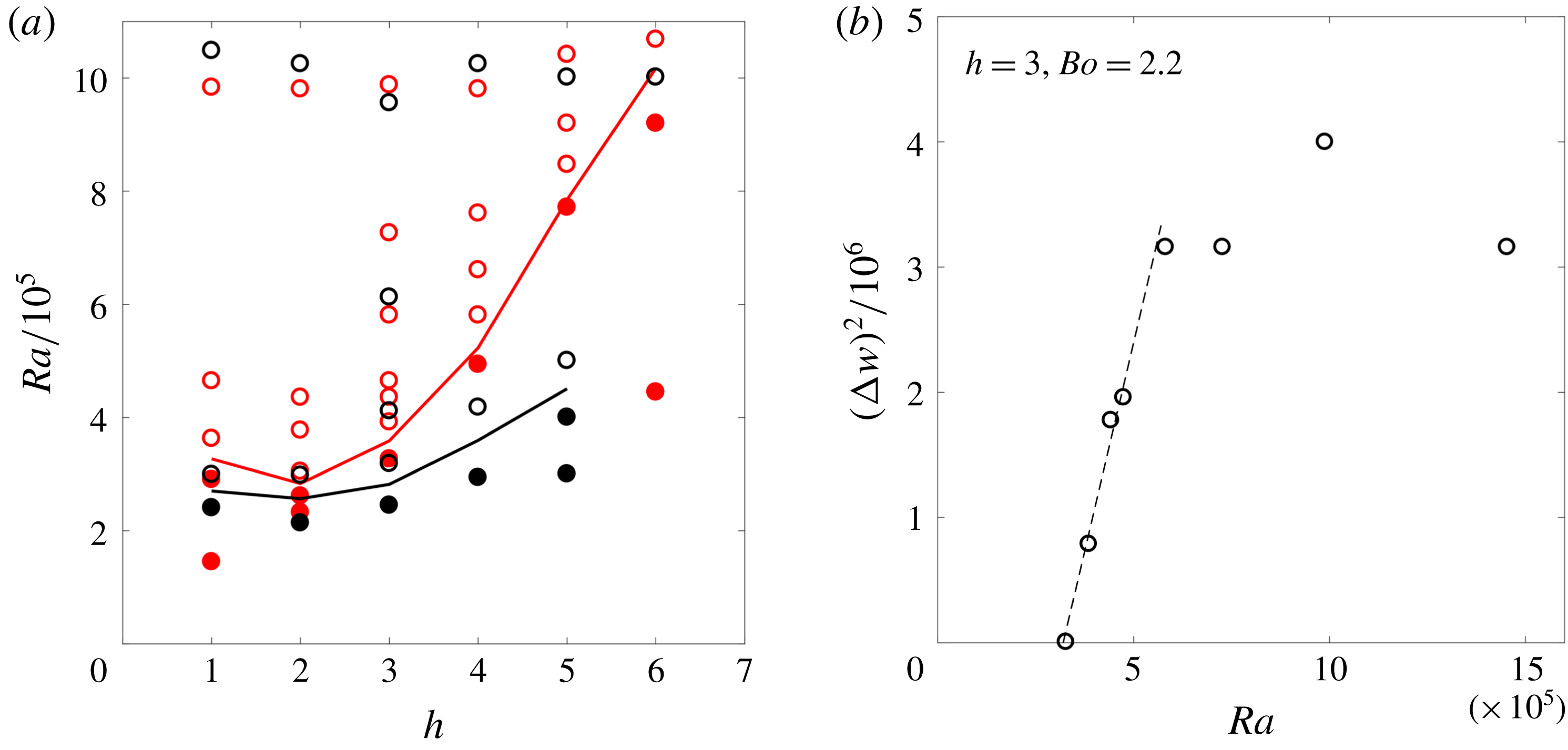
3.6 Stability diagram and nonlinear saturation amplitude
(a) Stability diagram in the
 $(h,Ra)$
space for
 $Bo=2.2$
(
 $R_{c}=4$
mm, red circles) and
 $Bo=4.8$
(
 $R_{c}=6$
mm, black circles). The points corresponding to a stable (respectively unstable) situation are plotted as solid (respectively open) symbols. Stable and unstable domains are separated by a solid line. (b) Bifurcation diagram showing the saturation amplitude as a function of the Rayleigh number for
 $Bo=2.2$
and
 $h=3$
. The dashed line corresponds to a Hopf bifurcation with
 $\unicode[STIX]{x0394}w=3.65\,(Ra-Ra_{c})^{1/2}$
. The error on
 $(\unicode[STIX]{x0394}w)^{2}$
is of the order of 30 %.

The instability described above only occurs for large enough values of the Rayleigh number. Below a critical Rayleigh number, the plume remains nearly steady until the end of the experiment – i.e. until complete saturation of the water in
 $\text{CO}_{2}$
(according to Henry’s law). The stability of the quasi-steady base flow has been investigated in the plane
 $(h,\,Ra)$
for two different Bond numbers. As shown in figure 10(a), the critical Rayleigh number
 $Ra_{c}$
depends on both the aspect ratio
 $h$
and the Bond number. The critical Rayleigh number has a minimum at
 $h\simeq 2$
, so that the flow is unconditionally stable for
 $Ra\lesssim 2.5\times 10^{5}$
. When the aspect ratio
 $h$
increases from 2 to 6, the critical Rayleigh number increases by a factor 2 if
 $Bo=2.2$
and by a factor 4 if
 $Bo=4.8$
. It seems that the meniscus (which is more curved at smaller Bond number) tends to stabilise the flow, which is consistent with the interpretation provided in § 3.5. Unfortunately, the stability diagram could not be obtained experimentally at higher Bond numbers, due to residual motions (a slow clockwise recirculating roll invading the whole cell, possibly due to a laser induced temperature asymmetry) which perturbed the onset of the instability.
A bifurcation diagram is presented in figure 10(b) for the particular values of the parameters
 $Bo=2.2$
and
 $h=3$
. For this purpose, the nonlinear amplitude of the oscillations
 $\unicode[STIX]{x0394}w$
is extracted in the experiments as the mean amplitude over 5 periods around the maximal amplitude (i.e. at the beginning of stage IV). The square of the saturation amplitude
 $\unicode[STIX]{x0394}w$
is then plotted as a function of the Rayleigh number. Despite the few experimental points and the quite large uncertainty on the measurements, the bifurcation appears to be supercritical. Close to the critical Rayleigh number
 $Ra_{c}$
, the amplitude
 $\unicode[STIX]{x0394}w$
is proportional to
 $(Ra-Ra_{c})^{1/2}$
(Hopf bifurcation).
4 Possible origin of the instability – heuristic model and discussion
As an interpretation of the observations, we propose a scenario in which the progressive filling of the cylinder by the
 $\text{CO}_{2}$
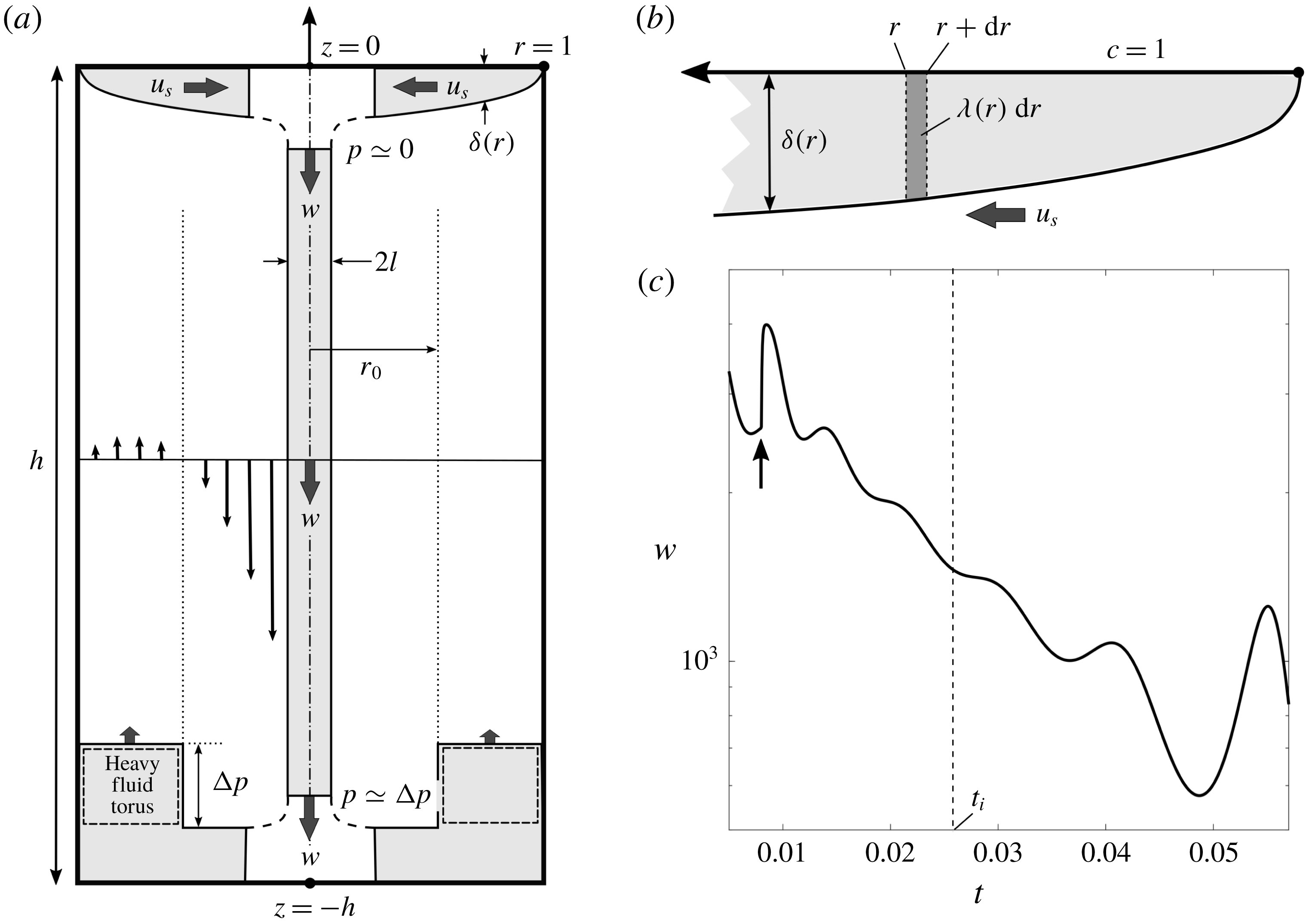
-enriched heavy fluid triggers the destabilisation. Such an interpretation is supported by a model with a reduced number of degrees of freedom, which has some similarities with the Lorentz waterwheel (Kolář & Gumbs Reference Kolář and Gumbs1992). The waterwheel corresponds to the streamline located beneath the free surface and inside the plume (see figure 11
a). This streamline is rectangular since the meniscus is assumed to be flat (i.e. the Bond number is assumed to be infinite).
(a) Explanatory sketch of the model (see text for explanations). (b) Zoom of the fluid zone beneath the free surface. (c) Typical evolution in time of the velocity for
 $Ra=10^{6}$
and
 $h=6$
. When a perturbative step (black arrow) is applied at
 $t=0.008$
, the resulting oscillation amplitudes first decay and then grow again as soon as
 $t>t_{i}\simeq 0.027$
.

When the fluid flows below the free surface (from
 $r=1$
to
 $r=0$
) at the velocity
 $u_{s}$
, carbon dioxide diffuses into the liquid, creating a thin layer of thickness
 $\unicode[STIX]{x1D6FF}(r,t)$
which increases as
 $r$
decreases (see figure 11
a). An equation for
 $\unicode[STIX]{x1D6FF}$
(and alternately for the linear density
 $\unicode[STIX]{x1D706}$
, see figure 11
b) can be obtained from the advection–diffusion equation for
 $c$
and from the incompressibility condition (see appendix A). Once the fluid reaches the axis of the cylinder, it sinks down to the bottom of the cell under the effect of gravity without loss of buoyancy. The
 $\text{CO}_{2}$
-enriched fluid forms a dense vertical shaft, which is subject to a viscous force from the surrounding fluid as it travels down towards the bottom wall. Unlike heat (Lopez & Marques Reference Lopez and Marques2013), the carbon dioxide is confined in the cylinder and cannot escape through the walls. Carbon dioxide is advected again upwards to the free surface once it has reached the bottom wall. A cylindrical annulus of
 $\text{CO}_{2}$
-enriched heavy fluid then builds up close to the lateral wall (labelled heavy fluid torus in figure 11
a), which exerts a counter force on the axial shaft and slows down the central plume. The differential equation for the velocity of the plume
 $w$
is obtained by calculating the momentum balance on the plume (again see appendix A). This axial velocity governs the recirculation of the flow and thus governs the radial velocity at the free surface
 $u_{s}$
.
The destabilisation of the flow can be understood as follows. Once the downward flow is slow enough, the boundary layer located beneath the free surface becomes overloaded. This excess of buoyancy then re-accelerates the fluid when it reaches the axis of the cylinder, thereby feeding the upward flowing zone and so on. The details of the derivation of the model and the subsequent linear stability analysis are given in appendix A. The model generally captures the essential features of the experimental phenomenology and yields reasonable trends and orders of magnitude for the frequency, phase velocity, wavenumber and onset time. Below are listed the main results obtained from a direct numerical integration of the system of equations (A 5) and (A 7)–(A 10) and from a linear stability analysis of these equations.
(i) The system switches from stable to unstable at a specific onset time
 $t_{i}$
, after a quasi-stationary regime where the velocity decreases. The time at which the change of regime occurs can be identified in the model by applying a small perturbative step just before the onset time. The oscillatory response is first damped and then grows again as soon as
$t>t_{i}$
(see figure 11
c). The so-determined value of the onset time is robust regarding the amplitude of the perturbation and the time at which the perturbation is applied.
(ii) The destabilisation of the flow in the model can be predicted analytically in the quasi-steady state approximation by calculating the growth rate using a linear stability analysis (see appendix A.4). This prediction is in excellent agreement with the direct numerical integration of the theoretical model.
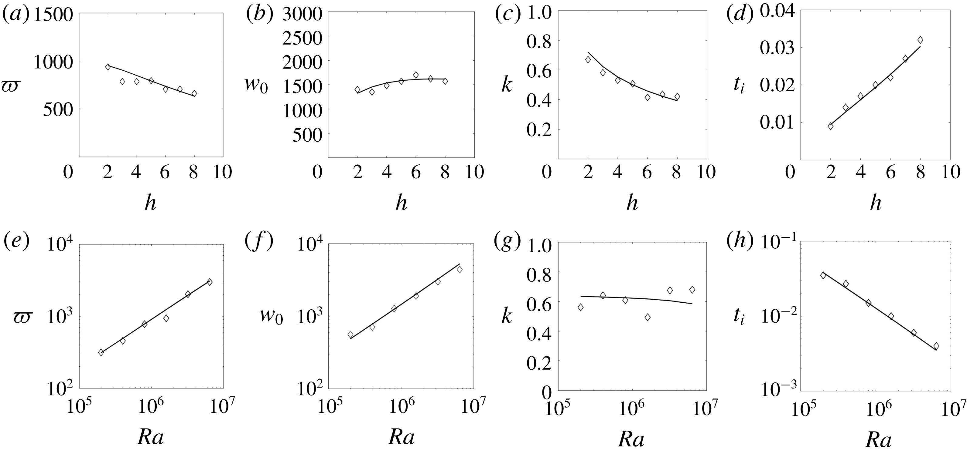
(iii) The dependences on Rayleigh number of the frequency, phase velocity, wavenumber and onset time are in very good agreement with the experimental observations: the scaling exponents provided by the model are very close to their experimental counterparts. For instance the frequency and the phase velocity scale as
$Ra^{3/4}$
in the experiments whereas they scale as
$Ra^{0.67}$
in the model for the range of Rayleigh numbers considered here (see § A.5). The onset time scales as
$Ra^{-0.55}$
in the experiments close to the model which predicts a scaling as
$Ra^{-0.67}$
in the range of the experiments. It can be noted that the model predicts different scalings for larger Rayleigh numbers (equal to
$Ra^{\pm 2/5}$
for infinite Rayleigh numbers).(iv) The model predicts a very small dependence of the frequency, phase velocity and wavenumber with the aspect ratio
$h$
. This is consistent with the experiments where their variations are smaller than the uncertainty in the measurements.(v) The model predicts that the onset time
$t_{i}$
is almost proportional to the aspect ratio
$h$
. This is again in excellent agreement with the experimental results.(vi) The values of the frequency
$\unicode[STIX]{x1D71B}$
, phase velocity
$w_{\unicode[STIX]{x1D719}}$
, wavenumber
$k$
and onset time are consistent with those experimentally observed (again, see § A.5) despite an underestimation of a factor between 2 and 6 for
$\unicode[STIX]{x1D71B}$
,
$w_{\unicode[STIX]{x1D719}}$
and
$k$
.


5 Conclusion
This paper presents experimental and numerical results on the destabilisation of a negatively buoyant plume created by an extended source at high Schmidt number. Such a configuration usually generates several plumes which interact in a complex way. Here, the presence of a meniscus confines the buoyant fluid into a unique axisymmetric plume, the stability of which can thus be analysed through reproducible experiments. After a long onset time, the quasi-steady plume destabilises through an axisymmetric puffing instability with an amplitude which saturates and decreases slowly at very late stages. Fortunately, most characteristics of the instability (frequency and wavenumber) are found to be independent of the size of the meniscus allowing for an extrapolation of the results to a flat surface (
 $Bo\rightarrow \infty$
).
The instability is related to the feedback of the global flow on the injection rate of buoyancy and to the presence of a background stratification. First, the feedback mechanism is due to the boundary condition of constant concentration at the surface (rather than a steady flux of carbon dioxide). A deceleration of the global flow within the container allows for a larger accumulation of buoyant fluid at the surface. When this added buoyancy reaches the axis of the cylinder, it brings an increase of the buoyant force which induces an acceleration of the global flow half a period later. This feedback mechanism sets the wavelength of the instability which is proportional to the radius of the cylinder. The perturbation is then advected by the flow at the velocity of the base flow which has been shown by Nadal et al. (Reference Nadal, Meunier, Pouligny and Laurichesse2013) to be proportional to
 $Ra^{2/3}(\log Ra)^{1/3}$
. Therefore, the frequency of the instability is proportional to
 $Ra^{2/3}(\log Ra)^{1/3}$
as well. Second, the background stratification builds up within the container due to the no-flux boundary conditions at the bottom and on the sides of the container. The time for the stratification to reach the buoyant surface is proportional to the height of the cylinder such that the onset time of the instability is also proportional to the height of the container. A simple heuristic model has been derived where the buoyant fluid is advected by the flow as in a water-wheel model. This model supports the idea that the background stratification is a key ingredient for the instability.
As discussed in the introduction, the nature of the instability has been found to be very different depending on the configuration of the system. In our case, the instability is a varicose puffing rather than a sinuous buckling. This is similar to what has been obtained for helium jets by Subbarao & Cantwell (Reference Subbarao and Cantwell1992), Cetegen & Kasper (Reference Cetegen and Kasper1996) and Cetegen et al. (Reference Cetegen, Dong and Soteriou1998). However, their scaling of the frequency as a function of the Richardson number cannot be extrapolated to our study since our configuration corresponds to an infinite Richardson number. The axisymmetric puffing instability observed in our study is also similar to the instability observed experimentally by Torrance et al. (Reference Torrance, Orloff and Rockett1969) and numerically by Lopez & Marques (Reference Lopez and Marques2013) for a point source of thermal buoyancy in a confined geometry. In both studies, the background stratification and the feedback mechanisms are present although not highlighted. It is thus natural to infer that the varicose nature of the instability is related to these two key ingredients. However, in our configuration (with stratification and feedback), preliminary results for large aspect ratios (
 $h>6$
) have revealed the presence of a weak sinuous instability. A possible explanation may lie in the vertical confinement of the plume. Indeed, the varicose instability has mostly been obtained in vertically confined containers (Torrance et al.
Reference Torrance, Orloff and Rockett1969; Lopez & Marques Reference Lopez and Marques2013) whereas sinuous instabilities have been obtained in open configurations (Kimura & Bejan Reference Kimura and Bejan1983; Pesci et al.
Reference Pesci, Porter and Goldstein2003). In our experiments, the plume is confined vertically for moderate aspect ratios, which is consistent with the observed axisymmetric varicose instability. For large aspect ratios (
 $h>6$
), the sinuous instability has a wavelength larger than for the varicose instability. Thus, the sinuous instability may be stabilised by the vertical confinement because its wavelength does not fit within the container.
Acknowledgements
The Agence Nationale de la Recherche (ANR) under the grant CO2-3D and the Labex MEC are acknowledged for financial support.
Supplementary movie
Supplementary movie is available at https://doi.org/10.1017/jfm.2018.564.
Appendix A. Axisymmetric model
A.1 Governing equations at the surface
As shown on the schematic drawing of figure 11, the velocity
 $u_{s}$
of the fluid at the free surface creates a thin layer of
 $\text{CO}_{2}$
enriched fluid, whose thickness becomes larger close to the centre. The concentration of
 $\text{CO}_{2}$
is governed by (2.3) which can be transformed into a radial equation at the free surface:
 $$\begin{eqnarray}\frac{\unicode[STIX]{x2202}c}{\unicode[STIX]{x2202}t}+u_{s}\frac{\unicode[STIX]{x2202}c}{\unicode[STIX]{x2202}r}-\frac{z}{r}\frac{\unicode[STIX]{x2202}ru_{s}}{\unicode[STIX]{x2202}r}\frac{\unicode[STIX]{x2202}c}{\unicode[STIX]{x2202}z}=\frac{\unicode[STIX]{x2202}^{2}c}{\unicode[STIX]{x2202}z^{2}}\end{eqnarray}$$
subject to the boundary condition
 $c=1$
at
 $z=0$
and
 $c=0$
at
 $z=-\infty$
.
This equation is valid for a free-slip boundary condition at the free surface since the velocity
 $u_{s}$
is uniform inside the diffusive layer. The model has thus been derived for free-slip boundary conditions. Surprisingly, this equation is also valid for a no-slip boundary condition at the free surface because the thickness of the viscous boundary layer is much smaller than the thickness of the diffusive layer of concentration. This is counter-intuitive in our case because the Schmidt number is very large (
 $S=550$
). However, Nadal et al. (Reference Nadal, Meunier, Pouligny and Laurichesse2013) found numerically that the viscous layer is 2–3 times smaller than the diffusive chemical layer (see their figure 15b).
As shown in the steady case by Whittaker & Lister (Reference Whittaker and Lister2006b ), a self-similar solution exists, of the form
 $$\begin{eqnarray}c(r,z,t)=1-\text{erf}\left[\frac{z}{\unicode[STIX]{x1D6FF}(r,t)}\right],\end{eqnarray}$$
with a thickness
 $\unicode[STIX]{x1D6FF}$
of the diffusive layer depending on
 $r$
. This result can be extended to an unsteady velocity profile with a thickness
 $\unicode[STIX]{x1D6FF}(r,t)$
depending on
 $r$
and
 $t$
by introducing (A 2) into (A 1). The thickness must then satisfy:
 $$\begin{eqnarray}\frac{\unicode[STIX]{x2202}\unicode[STIX]{x1D6FF}^{2}}{\unicode[STIX]{x2202}t}+\frac{1}{r^{2}u_{s}}\frac{\unicode[STIX]{x2202}(ru_{s}\unicode[STIX]{x1D6FF})^{2}}{\unicode[STIX]{x2202}r}=4.\end{eqnarray}$$
It is possible to define the linear density of
 $\text{CO}_{2}$
concentration
 $$\begin{eqnarray}\unicode[STIX]{x1D706}(r,t)=\int _{0}^{\infty }2\unicode[STIX]{x03C0}rc(r,z,t)=2\unicode[STIX]{x03C0}r\unicode[STIX]{x1D6FF}(r,t)Q\quad \text{with}\;Q=\int _{0}^{\infty }[1-\text{erf}(x)]\,\text{d}x=0.5642.\end{eqnarray}$$
Introducing this definition into (A 3) gives an equation for
 $\unicode[STIX]{x1D706}$
at the free surface
 $$\begin{eqnarray}\frac{\unicode[STIX]{x2202}\unicode[STIX]{x1D706}^{2}}{\unicode[STIX]{x2202}t}+\frac{1}{u_{s}}\frac{\unicode[STIX]{x2202}(u_{s}^{2}\unicode[STIX]{x1D706}^{2})}{\unicode[STIX]{x2202}r}=16\unicode[STIX]{x03C0}^{2}r^{2}Q^{2}.\end{eqnarray}$$
For a steady plume, Nadal et al. (Reference Nadal, Meunier, Pouligny and Laurichesse2013) showed using a matched asymptotic expansion that the velocity at the surface
 $u_{s}$
is proportional to the plume velocity
 $w$
and can be approximated by:
 $$\begin{eqnarray}u_{s}(r)=-\unicode[STIX]{x1D705}w(1-r),\end{eqnarray}$$
with the constant
 $\unicode[STIX]{x1D705}\sim 0.25$
around
 $Ra=10^{6}$
. This formula is valid theoretically in the limit of large aspect ratios
 $h$
for a steady plume. Experimentally, it was found to be independent of
 $h$
for
 $h>3$
. We will keep this profile of radial velocity at the free surface which is valid for a nearly parallel plume, in the limit of low wavenumber of the perturbation and in the case of free-slip boundary conditions at the free surface.
A.2 Equations inside the plume
When reaching the axis of the cylinder, the linear density of
 $\text{CO}_{2}$
is then advected at the velocity of the plume
 $w(t)$
which is supposed to be invariant in
 $z$
. The equation for
 $\unicode[STIX]{x1D706}(z,t)$
inside the plume is thus
 $$\begin{eqnarray}\frac{\unicode[STIX]{x2202}\unicode[STIX]{x1D706}}{\unicode[STIX]{x2202}t}+w\frac{\unicode[STIX]{x2202}\unicode[STIX]{x1D706}}{\unicode[STIX]{x2202}z}=0.\end{eqnarray}$$
The continuity condition between the free surface and the vertical plume is found by equating the incoming flux at the free surface with the downward flux at the top of the plume:
 $$\begin{eqnarray}\left[\unicode[STIX]{x1D706}(r,t)u_{s}\right]_{r=0}=\left[\unicode[STIX]{x1D706}(z,t)w\right]_{z=h}\!.\end{eqnarray}$$
The exact downward flux at
 $z=h$
can be calculated in a more rigorous way by taking into account the Gaussian profile of concentration
 $c(r)$
and its associated profile of axial velocity. Nadal et al. (Reference Nadal, Meunier, Pouligny and Laurichesse2013) showed numerically (see their figure 11a) that for a steady plume at large Prandtl number, the concentration is Gaussian (of size
 $l$
) in the radial direction and nearly uniform in the axial direction. Assuming that there is no axial flux, the velocity profile can be calculated as
 $w\,F_{l}(r)/F_{l}(0)$
where
 $$\begin{eqnarray}F_{l}(r)=\int _{r/l}^{1/l}\frac{1-e^{-x^{2}}}{x}\,\text{d}x+(r^{2}-1)(1-l^{2}).\end{eqnarray}$$
Such a profile depends logarithmically on the thickness of the plume
 $l$
. In our model,
 $l$
was chosen equal to 0.1, which is characteristic of the range of Rayleigh numbers found in the experiment. Taking into account this velocity profile would alter the value of the flux by 20 % only, since the profile of velocity is much thicker than the profile of concentration. Taking into account this effect would modify by 15 % the frequency and the velocity of the instability. It has been neglected here for simplicity.
Finally, the velocity of the plume is subject to different forces which correspond to the different terms of equation (2.1). The latter can be found by integrating equation (2.1) multiplied by
 $r$
from
 $z=0$
to
 $z=h$
and from
 $r=0$
to
 $r=r_{0}$
(which corresponds to the radius where the flow is reversed). To perform the integration, we have assumed that the velocity profile was close to the profile of a steady plume (A 9). The value of the reversing radius
 $r_{0}$
was chosen as
 $r_{0}=0.3$
since it varies from 0.4 down to 0.2 during an experiment. This value has almost no influence on the characteristics of the instability (wavenumber, frequency) but it slightly modifies the value of the onset time of the instability. So, after integrating
 $r\times$
(2.1), one gets the momentum balance equation
 $$\begin{eqnarray}\frac{I}{S}\frac{\text{d}w}{\text{d}t}+Dw=\frac{-Ra}{h}\left(\int _{0}^{h}\unicode[STIX]{x1D706}(z)\,\text{d}z-B\int _{0}^{t}\unicode[STIX]{x1D706}w\,\text{d}t\right)\!.\end{eqnarray}$$
In equation (A 10):
(i) The inertia of the plume
$h(I/S)(\text{d}w/\text{d}t)$
(where
$I=\int _{0}^{r_{0}}2\unicode[STIX]{x03C0}rF_{l}(r)\,\text{d}r/F_{l}(0)\simeq 0.124$
) comes from the first term of equation (2.1).(ii) The term
$BRa\int _{0}^{t}\unicode[STIX]{x1D706}w\,\text{d}t$
(where
$B=r_{0}^{2}/(1-r_{0}^{2})\simeq 0.1$
) corresponds to the mean adverse pressure gradient due to the
$\text{CO}_{2}$
filling of the outer part of the cylinder (
$r_{0}<r<1$
).(iii) The term
$Ra\int _{0}^{h}\unicode[STIX]{x1D706}(z)\,\text{d}z$
is the weight of the plume.(iv) The drag
$-Dhw$
(where
$D=2\unicode[STIX]{x03C0}(1-2r_{0}^{2})/F_{l}(0)\simeq 3.24$
) corresponds to the last (viscous) term of equation (2.1).







Two remarks may be formulated concerning the previous analysis. First, the second term of (2.1) leads to zero for a parallel plume. Secondly, the weight of the heavy layer located underneath the free surface is neglected compared to the weight of the plume. This approximation is valid in the limit of large cylinder’s height
 $h$
since the weight of the plume is proportional to
 $h$
. In our experiments, this assumption seems to be justified since the laminar velocity of the plume was measured to be independent of the Bond number (see Nadal et al.
Reference Nadal, Meunier, Pouligny and Laurichesse2013) whereas the forcing due to the heavy layer is proportional to the tilt of the free surface which depends on the curvature of the meniscus, i.e. on the Bond number.
The model can be solved numerically by integrating equations (A 5) and (A 7) together with the continuity condition (A 8) between the two domains. The velocity of the plume is found numerically by integrating equation (A 10) and is in fair agreement with the experimental and numerical results. After a rapid acceleration of the plume velocity, the plume enters a quasi-stationary regime where the plume velocity gradually diminishes due to the filling up of the cylinder. After a long onset time, the plume becomes unstable (see the plot of the plume velocity in figure 11 c where the perturbations are damped and then grow again after the onset time). The perturbations grow in amplitude, but do not saturate as in the experiment and in the numerical simulations.
In the following, we present a linear stability analysis of the model and the corresponding orders of magnitude and scaling laws for the wavenumber, the frequency and the onset time of the instability.
A.3 Base flow (QSSA)
We first try to find the stable solution, obtained in the quasi-steady state approximation (QSSA). Assuming that the variables evolve on a slow time, the temporal derivative in (A 5) can be neglected such that the solution for the linear density at the free surface can be calculated as:
 $$\begin{eqnarray}\unicode[STIX]{x1D706}_{0}(r)=2\unicode[STIX]{x03C0}Q\left(\frac{1+2r+3r^{2}}{3\unicode[STIX]{x1D705}w_{0}}\right)^{1/2}.\end{eqnarray}$$
Here the index
 $0$
refers to the QSSA regime.
Inside the plume, the linear density of scalar is constant, as found by integrating (A 7). Its value is found using the jump condition (A 8) and the ratio
 $u_{s}/w=\unicode[STIX]{x1D705}$
given by (A 6) for
 $r=0$
and one gets
 $$\begin{eqnarray}\unicode[STIX]{x1D706}_{0}(z)=2\unicode[STIX]{x03C0}Q\sqrt{\frac{\unicode[STIX]{x1D705}}{3w_{0}}}.\end{eqnarray}$$
Introducing this expression in the balance of momentum (while neglecting the time derivative) leads to an equation for the plume velocity in the QSSA
 $$\begin{eqnarray}Dw_{0}=2\unicode[STIX]{x03C0}QRa\sqrt{\frac{\unicode[STIX]{x1D705}}{3w_{0}}}-\frac{BRa}{h}\int _{0}^{t}2\unicode[STIX]{x03C0}Q\sqrt{\unicode[STIX]{x1D705}w_{0}/3}\,\text{d}t.\end{eqnarray}$$
This can be solved by differentiation and gives the time as a function of the velocity:
 $$\begin{eqnarray}t=\frac{hD}{BRa^{2/3}}\left[\frac{3^{4/3}D}{2\unicode[STIX]{x1D705}^{1/3}(2\unicode[STIX]{x03C0}Q)^{2/3}}+\frac{Ra^{2/3}}{2w_{0}}-\frac{D\sqrt{3w_{0}}}{\unicode[STIX]{x03C0}Q\sqrt{\unicode[STIX]{x1D705}}Ra^{1/3}}\right].\end{eqnarray}$$
A.4 Linear stability analysis
A small perturbation is then added to the base flow of the QSSA
 $$\begin{eqnarray}\displaystyle & \displaystyle \unicode[STIX]{x1D706}=\unicode[STIX]{x1D706}_{0}\left[1+\unicode[STIX]{x1D716}\unicode[STIX]{x1D706}_{1}e^{\unicode[STIX]{x1D70E}t}\right], & \displaystyle\end{eqnarray}$$
 $$\begin{eqnarray}\displaystyle & \displaystyle w=w_{0}\left[1+\unicode[STIX]{x1D716}w_{1}e^{\unicode[STIX]{x1D70E}t}\right], & \displaystyle\end{eqnarray}$$
where
 $\unicode[STIX]{x1D716}$
is the initial amplitude of the perturbation. Introducing this expansion into the surface equation (A 5) yields the equation for
 $\unicode[STIX]{x1D706}_{1}(r)$
, valid at
 $O(\unicode[STIX]{x1D716})$
:
 $$\begin{eqnarray}\unicode[STIX]{x1D70E}\unicode[STIX]{x1D706}_{1}-\unicode[STIX]{x1D705}w_{0}(1-r)\frac{\unicode[STIX]{x2202}\unicode[STIX]{x1D706}_{1}}{\unicode[STIX]{x2202}r}+16\unicode[STIX]{x03C0}^{2}Q^{2}r^{2}\frac{\unicode[STIX]{x1D706}_{1}}{\unicode[STIX]{x1D706}_{0}^{2}}=-\frac{8\unicode[STIX]{x03C0}^{2}Q^{2}r^{2}w_{1}}{\unicode[STIX]{x1D706}_{0}^{2}}.\end{eqnarray}$$
The homogeneous solution
 $\unicode[STIX]{x1D706}_{1}^{h}$
of this equation is equal to
 $$\begin{eqnarray}\unicode[STIX]{x1D706}_{1}^{h}=\frac{(1-r)^{-2-\unicode[STIX]{x1D70E}/\unicode[STIX]{x1D705}w_{0}}}{1+2r+3r^{2}}\end{eqnarray}$$
from which the full solution can be found by varying the constant, leading (after integration from
 $r=0$
to
 $r=1$
) to the value of the linear density on the axis:
 $$\begin{eqnarray}\unicode[STIX]{x1D706}_{1}(r=0)=-\frac{12w_{1}}{(2+\tilde{\unicode[STIX]{x1D70E}})(3+\tilde{\unicode[STIX]{x1D70E}})(4+\tilde{\unicode[STIX]{x1D70E}})}.\end{eqnarray}$$
Here, the growth rate has been re-dimensionalised as
 $$\begin{eqnarray}\tilde{\unicode[STIX]{x1D70E}}=\frac{\unicode[STIX]{x1D70E}}{\unicode[STIX]{x1D705}w_{0}}.\end{eqnarray}$$
Inside the plume, the equation for the linear density (A 7) at order
 $O(\unicode[STIX]{x1D716})$
indicates that the linear density
 $\unicode[STIX]{x1D706}_{1}$
is just advected by the base flow:
 $$\begin{eqnarray}\unicode[STIX]{x1D70E}\unicode[STIX]{x1D706}_{1}+w_{0}\frac{\unicode[STIX]{x2202}\unicode[STIX]{x1D706}_{1}}{\unicode[STIX]{x2202}z}=0.\end{eqnarray}$$
This is indeed what is observed experimentally (see § 3.4). The linear density at order
 $O(\unicode[STIX]{x1D716})$
in the plume can be calculated by using the continuity condition (A 8) at order
 $O(\unicode[STIX]{x1D716})$
and the value (A 19) of the linear density at the centre of the free surface:
 $$\begin{eqnarray}\unicode[STIX]{x1D706}_{1}(z)=-\frac{12w_{1}}{(\tilde{\unicode[STIX]{x1D70E}}+2)(\tilde{\unicode[STIX]{x1D70E}}+3)(\tilde{\unicode[STIX]{x1D70E}}+4)}e^{\unicode[STIX]{x1D70E}(z-h)/w_{0}}.\end{eqnarray}$$
Introducing this expression in the balance of momentum (A 10) at order
 $O(\unicode[STIX]{x1D716})$
leads to the dispersion relation for the growth rate
 $\tilde{\unicode[STIX]{x1D70E}}$
:
 $$\begin{eqnarray}\frac{\unicode[STIX]{x1D705}w_{0}I}{S}\tilde{\unicode[STIX]{x1D70E}}+D=\frac{2\unicode[STIX]{x03C0}QRa}{h\sqrt{3\unicode[STIX]{x1D705}}w_{0}^{3/2}\tilde{\unicode[STIX]{x1D70E}}}A\quad \text{with}~A=-\frac{12(1-e^{-\unicode[STIX]{x1D705}\tilde{\unicode[STIX]{x1D70E}}h})}{(\tilde{\unicode[STIX]{x1D70E}}+2)(\tilde{\unicode[STIX]{x1D70E}}+3)(\tilde{\unicode[STIX]{x1D70E}}+4)}.\end{eqnarray}$$
This equation has first been analysed numerically. It was found that the real part is always negative when the velocity
 $w_{0}$
is equal to its initial value obtained before the build-up of the background stratification. This clearly proves that the background stratification is a necessary condition for the destabilisation of the system.
In the QSSA, the velocity
 $w_{0}$
evolves slowly such that the real part of the growth rate increases slowly with time. The instability starts at the onset time when the real part of the growth rate reaches 0, i.e. when the growth rate is purely imaginary (
 $\tilde{\unicode[STIX]{x1D70E}}=\text{i}\tilde{\unicode[STIX]{x1D71B}}$
), which leads to two real equations by taking the real part and imaginary part of the dispersion relation (A 23). Eliminating
 $w_{0}$
from these equations permits to calculate the frequency
 $\tilde{\unicode[STIX]{x1D71B}}$
at the onset of the instability. It is found as the root of
 $$\begin{eqnarray}4\unicode[STIX]{x03C0}^{2}Q^{2}\unicode[STIX]{x1D705}^{2}I^{3}\tilde{\unicode[STIX]{x1D71B}}A_{i}^{5}Ra^{2}+3h^{2}S^{3}D^{5}A_{r}^{3}=0,\end{eqnarray}$$
where
 $A_{r}$
and
 $A_{i}$
denote the real part and imaginary part of
 $A$
defined in (A 23) in which
 $\tilde{\unicode[STIX]{x1D70E}}$
is replaced by
 $\text{i}\tilde{\unicode[STIX]{x1D71B}}$
. The velocity of the plume at onset can then be calculated by taking the imaginary part of (A 23):
 $$\begin{eqnarray}w_{0}=\left(\frac{-2\unicode[STIX]{x03C0}QRaSA_{r}}{h\sqrt{3}\unicode[STIX]{x1D705}^{3/2}I\tilde{\unicode[STIX]{x1D71B}}^{2}}\right)^{2/5}.\end{eqnarray}$$
We recall here that the frequency has been rescaled as
 $\unicode[STIX]{x1D71B}=\tilde{\unicode[STIX]{x1D71B}}\unicode[STIX]{x1D705}w_{0}$
. The wavenumber of the instability is simply obtained as
 $k=\unicode[STIX]{x1D71B}/w_{0}$
. The onset time can then be calculated by introducing the previous expression of
 $w_{0}$
into (A 14).
It can be derived asymptotically that, for large Rayleigh numbers, the wavenumber
 $k$
is independent of the Rayleigh number whereas the frequency
 $\unicode[STIX]{x1D71B}$
and the plume velocity
 $w_{0}(t_{i})$
scale as
 $Ra^{2/5}$
. Indeed, (A 24) indicates that
 $A_{i}$
tends to 0 because
 $A_{r}$
and
 $\tilde{\unicode[STIX]{x1D71B}}$
must be finite (since
 $\tilde{\unicode[STIX]{x1D71B}}=0$
is not a solution and since
 $|A_{r}|<|A|<1$
). Assuming
 $A_{i}=0$
fixes the value of
 $\tilde{\unicode[STIX]{x1D71B}}$
as independent of the Rayleigh number, since it is solution of
 $$\begin{eqnarray}\text{Imag}\left[\frac{12(1-\text{e}^{-\unicode[STIX]{x1D705}\text{i}\tilde{\unicode[STIX]{x1D71B}}h})}{(\text{i}\tilde{\unicode[STIX]{x1D71B}}+2)(\text{i}\tilde{\unicode[STIX]{x1D71B}}+3)(\text{i}\tilde{\unicode[STIX]{x1D71B}}+4)}\right]=0,\end{eqnarray}$$
where
 $\text{Imag}$
stands for imaginary part of a number. The scalings of
 $w_{0}$
and then
 $\unicode[STIX]{x1D71B}$
are thus obtained directly from (A 25).
A.5 General trends and orders of magnitude
Frequency, phase velocity, wavenumber and onset time at the beginning of the instability predicted by the model as a function of
 $h$
for
 $Ra=10^{6}$
(a–d), and as a function of
 $Ra$
for
 $h=3$
(e–h). Symbols are obtained by solving numerically the model (A 5)–(A 10). Solid lines correspond to the linear stability analysis where the frequency and velocity at onset are given by (A 24), (A 25).

The frequency, wavenumber, phase velocity and onset time produced by the model are plotted in figure 12 as a function of the aspect ratio and the Rayleigh number. First, the analytical predictions (A 24), (A 25) using the linear stability analysis (plotted as solid lines) are in excellent agreement with the results obtained through a numerical integration of the model (plotted as symbols). Second, the general trends observed on the frequency, the wavenumber, the phase velocity and the onset time are consistent, although not in exact numerical accordance with the experiment.
The frequency
 $\unicode[STIX]{x1D71B}$
is an increasing function of the Rayleigh number in both the model and in the experiments. In the model, it scales as
 $Ra^{0.67}$
(see figure 12
b), close to the experimental scaling equal to
 $Ra^{3/4}$
. It should be noted that these scalings are obtained by fitting the theoretical predictions in the range where the experimental results have been obtained. However, the model predicts that the exponent is smaller at larger Rayleigh numbers (equal to
 $2/5$
in the limit of large Rayleigh numbers). In the model, the frequency
 $\unicode[STIX]{x1D71B}$
is a slightly decreasing function of the aspect ratio
 $h$
(by a factor 2 over one decade), whereas it appears almost independent of
 $h$
in the experiments. Finally, the orders of magnitude predicted by the model are correct for the frequency despite an underestimation by a factor 6.
At the onset of the instability, the phase velocity (which is equal to the plume velocity
 $w_{0}(t_{i})$
) is an increasing function of the Rayleigh number (scaling as
 $Ra^{0.67}$
in the range of the experiments) whereas its experimental counterpart scales as
 $Ra^{3/4}$
(see figure 8
b). As mentioned above, the model predicts a smaller scaling exponent equal to
 $2/5$
in the limit of large Rayleigh number. In the model, the phase velocity is a slowly increasing function of the aspect ratio (by 20 %). Even if not obvious in figure 8(a), such a trend is not inconsistent with that of the experimental phase velocity, the latter being marred by a large uncertainty. Finally, the orders of magnitude predicted by the model are correct for the phase velocity despite an underestimation by a factor 2.
The wavenumber is a decreasing function of the aspect ratio (by 50 %) and a slightly decreasing function of the Rayleigh number (by 10 % over two decades) while its experimental counterpart seems to be independent from both parameters. However, the large uncertainty in the experimental measurements (of the order of 30 %) may explain this apparent disagreement. Again the order of magnitude produced by the model for the wavenumber
 $k$
is consistent with the experimental one despite an underestimation by a factor 2.
Finally, the onset time is very well rendered by the model. In the model, it increases nearly proportionally to the aspect ratio
 $h$
as in the experiments (see figure 9
a). It is a decreasing function of the Rayleigh number (scaling as
 $Ra^{-0.67}$
) as in the experiments (where
 $t_{i}\propto Ra^{-0.55}$
in figure 9
b). Furthermore, there is a quantitative agreement (within 30 %) between the experiments and the model.