

Introduction
An enlarged vestibular aqueduct is a commonly detected imaging abnormality in computed tomography (CT) evaluations of children with sensorineural hearing loss (SNHL).Reference Mafong, Shin and Lalwani1–Reference Madden, Halsted, Benton, Greinwald and Choo3 Although the diameter of the aqueduct at the midpoint of the post-isthmic segment on axial images has been proposed as a potential diagnostic standard for an enlarged vestibular aqueduct, the measurement to be used as the standard remains inconsistent. The published values include 1.0 mm,Reference Boston, Halsted, Meinzen-Derr, Bean, Vijayasekaran and Arjmand2 1.4 mm,Reference Zalzal, Tomaski, Vezina, Bjornsti and Grundfast4 1.5 mm,Reference Valvassori and Clemis5–Reference Koesling, Rasinski and Amaya9 1.9 mmReference Arcand, Desrosiers, Dubé and Abela10 and 2.0 mm.Reference McClay, Tandy, Grundfast, Choi, Vezina and Zalzal11 Moreover, one report did not refer to the midpoint width, but rather defined a large vestibular aqueduct as one with a ‘visible large aperture (≥4 mm) and a small distance between the vestibule and traceable part of the vestibular aqueduct nearest to the vestibule (≥1 mm)’.Reference Okumura, Takahashi, Honjo, Takagi and Mitamura12 Another study considered the vestibular aqueduct to be enlarged if its diameter exceeded the diameter of one crus of the adjacent normal semicircular canal.Reference Weissman13 Though the causes of these inconsistencies remain unknown, they may be related to the course and morphology of the vestibular aqueduct, the technique used, and/or the site selected for measurement.
The vestibular aqueduct is a small bony canal that connects the vestibule to the cranial cavity. The vestibular aqueduct contains the endolymphatic duct and part of the endolymphatic sac. The shape of the vestibular aqueduct forms an inverted ‘J’, with a short ascending proximal segment and a longer distal descending segment. The proximal segment arises from the medial wall of the vestibule. As the aqueduct turns inferiorly, it narrows into an isthmus. The distal straight segment (i.e. the post-isthmic segment) enlarges along its inferior and posterior course, and ends as the external aperture on the posterior surface of the petrous pyramid.Reference Minerva, Mafee, Valvassori and Becker14 Although the post-isthmic segment forms a triangular slit,Reference Minerva, Mafee, Valvassori and Becker14 it is known that the vestibular aqueduct can appear tubular on routine axial images and images acquired in the 45° oblique plane.Reference Minerva, Mafee, Valvassori and Becker14 Currently, its appearance on other types of images remains unknown.
To date, most of the reported CT imaging data of the vestibular aqueduct have been based on measurements obtained on routine axial sections, with only a few studies examining the vestibular aqueduct using other types of sections.Reference Ozgen, Cunnane, Caruso and Curtin15, Reference Murray, Tanaka, Cameron and Gianoli16 However, axial sections are not ideal for assessing the anatomy and dimensions of the vestibular aqueduct owing to its oblique orientation. Thus, assessing the morphology of the vestibular aqueduct in other planes is essential. The present study aimed to identify and characterise the morphology of the vestibular aqueduct on axial, single-oblique and double-oblique CT images.
Materials and methods
Study population
Institutional research ethics review board approval was obtained for this study. Patient anonymity was maintained.
A search of our institution's medical records and radiology databases for consecutive patients who underwent CT scans of the temporal bone for reasons other than SNHL and vertigo attacks, from July 2009 through January 2011, revealed 115 patients. Patients were excluded if they had undergone previous surgery on the temporal bone that made the vestibular aqueduct difficult or impossible to identify (n = 1), or if the CT images were of poor quality (n = 2). The remaining 112 patients (62 men and 50 women; 224 ears), with a mean (± standard deviation (SD)) age of 41.76 ± 18.89 years (age range, 1–77 years), comprised our study population.
The CT examinations were performed for the following indications: otitis media (n = 33), trauma (n = 5), cholesteatoma (n = 51), conductive hearing loss (n = 11), mastoidectomy follow up (n = 5), facial nerve paralysis (n = 1), headache (n = 1), otalgia (n = 2), foreign bodies in the external acoustic meatus (n = 1) and external otitis (n = 2). We then assessed the audiological records of all the patients to ensure that none of them had SNHL.
Computed tomography scan protocol
All of the subjects were scanned with a 16-section, multi-detector CT scanner (Somatom Sensation 16; Siemens Medical Solutions, Forchheim, Germany). The head of each subject was placed in a neutral position, without chin tilt, to approximate the Reid base line. Both temporal bones were covered by the original scan. The axial images were acquired with the following parameters: slice thickness, 0.6 mm; increment, 0.3 mm; 120 kV; 150–350 mAs; pitch, 0.8; reconstruction kernel, B70; matrix, 512 × 512; and field of view, 300 mm. The image dataset was reconstructed to an 80 mm field of view, with an individual voxel size of 0.6 × 0.6 × 0.6 mm. Then, we used a workstation (Wizard; Siemens Medical Solutions) to obtain the multiplanar reformation images.
Data post-processing
The archived images in the Digital Imaging and Communications in Medicine format were transferred to a separate workstation (Volume; Siemens Medical Solutions). The images were rendered anonymous, with all clinical data, including the patients’ histories, removed. The images were presented in random order.
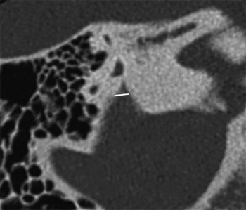
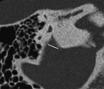
Because the proximal segment of a normal vestibular aqueduct is usually invisible, we used the distal segment for measurements. The single-oblique images were generated from the axial images by positioning the reference line through the midpoint of the vestibular aqueduct (Figure 1a). The double-oblique images were generated from the single-oblique images by positioning the reference line through the vestibular aqueduct (Figure 1b). The double-oblique images depict the normal anatomy of the vestibular aqueduct (Figure 1c). The single-oblique and double-oblique images for each ear were independently generated at the workstation by two radiologists (YQ and RG, with 6 and 16 years of experience with temporal bone CT images, respectively). The anatomical locations and orientations of the structures to be evaluated were confirmed on images in the axial and coronal planes of reference. The time required to post-process the CT image datasets was 2–3 minutes per ear.
Single-oblique and double-oblique images of the vestibular aqueduct. (a) Orthogonal axial reference image shows the reconstruction of the single-oblique image (white line) through the midpoint of the vestibular aqueduct. (b) Single-oblique image shows the reconstruction of the double-oblique image (white line) through the vestibular aqueduct. (c) Double-oblique image depicts normal anatomy of the vestibular aqueduct (arrow). The vestibular aqueduct was considered fissured because it was funnel-shaped in the double-oblique image, but tubular in the axial and single-oblique images.

Post-isthmic aqueduct measurements
The methodology for measuring the vestibular aqueduct was adapted from Vijayasekaran et al.Reference Vijayasekaran, Halsted, Boston, Meinzen-Derr, Bardo and Greinwald17 and Dewan et al.Reference Dewan, Wippold and Lieu18 (Figures 2 and 3). The images were magnified, and then we obtained two measurements of the aqueduct on each plane: a measurement at the approximate midpoint and a measurement at the external aperture. The measurements were manually obtained and calculated to the nearest 0.01 mm using electronic calipers. The measurements were performed by two radiologists (YQ and RG) and the averaged value was regarded as the final value.
The midpoint widths of the vestibular aqueduct are defined as the part of the vestibular aqueduct located half the distance in the petrous bone from its origin in the labyrinth to its aperture in the epidural space. The posterior wall of vestibule, or crus commune, was used in place of the origin of a normal aqueduct if it was invisible. The midpoint was measured on the image in which the width was largest.

The opercular widths of the vestibular aqueduct are measured by drawing a line from the opercular edge anterolaterally to form a 90° angle with the posterior wall of the petrous bone.

Midpoint measurement
The midpoint of the vestibular aqueduct in the axial, single-oblique and double-oblique images was defined as the part of the vestibular aqueduct located half of the distance in the petrous bone from its origin in the labyrinth to its aperture in the epidural space (Figure 2). We used the posterior wall of the vestibule or the crus commune in place of the origin of a normal aqueduct if the aqueduct was invisible. Measurements were obtained on the image with the largest midpoint width.
Opercular measurement
The opercular widths of the vestibular aqueduct were measured in the same plane by drawing a line from the opercular edge anterolaterally to form a 90° angle with the posterior wall of the petrous bone (Figure 3). Measurements were obtained on the CT image with the largest opercular width.
Morphology
We designated the vestibular aqueduct as funnel-shaped in terms of morphology when the size of the operculum was two times larger than the size of the midpoint in any one of the three image types. The vestibular aqueduct was considered invisible if it was difficult or impossible to identify on all of the axial, single-oblique and double-oblique images. The vestibular aqueduct was considered fissured if it was funnel-shaped in any one of the three image types, but tubular in the other two image types (Figure 1). The vestibular aqueduct was considered tubular if it was shaped like a tube in all of the axial, single-oblique and double-oblique images (Figure 4).
The vestibular aqueduct was considered tubular because it was shaped like a tube in all of the (a) axial, (b) single-oblique and (c) double-oblique images.

Statistical analysis
Numerical data are reported as means ± SDs. We compared the size of the vestibular aqueduct among the axial, single-oblique and double-oblique images using the Kruskal–Wallis test. If a significant difference was identified among the three image types, post-hoc pairwise comparisons were then performed using the Mann–Whitney U test with Bonferroni correction. Inter-observer agreement was assessed with the intraclass correlation co-efficient. Intraclass correlation co-efficient values of 0.41–0.60, 0.61–0.80, and 0.81 or higher indicated moderate agreement, substantial agreement and almost perfect agreement, respectively. In addition, the 95 per cent confidence intervals were assessed. The co-efficient of variation (equal to the SD divided by the mean) was calculated for each image type and anatomical location. The chi-square test was used for comparing categorical variables. Statistical analyses were performed with SPSS 16.0 software (IBM, Chicago, Illinois, USA) and GraphPad Prism software version 5.00 (San Diego, California, USA). Differences were considered significant at p < 0.05.
Results
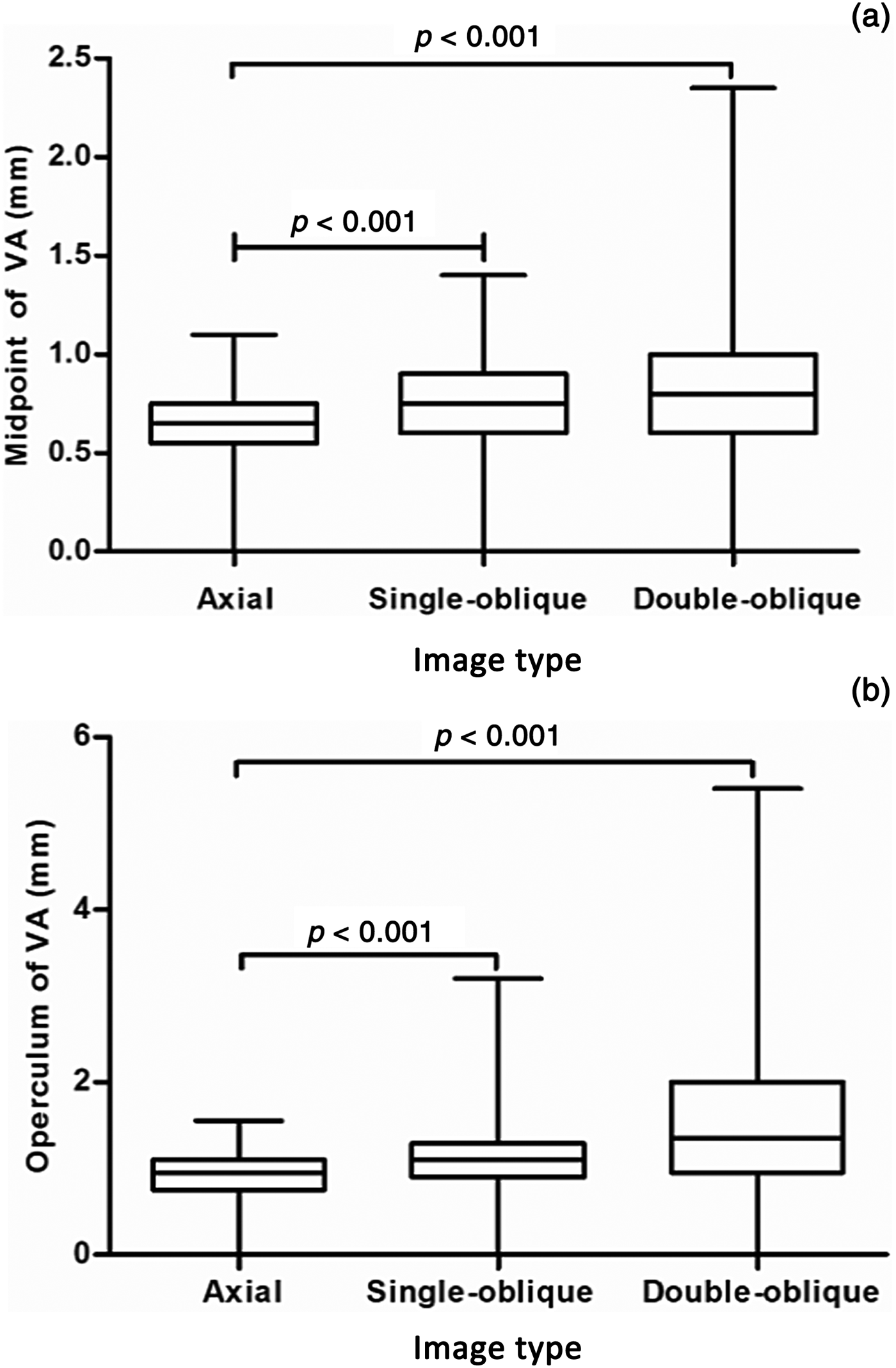
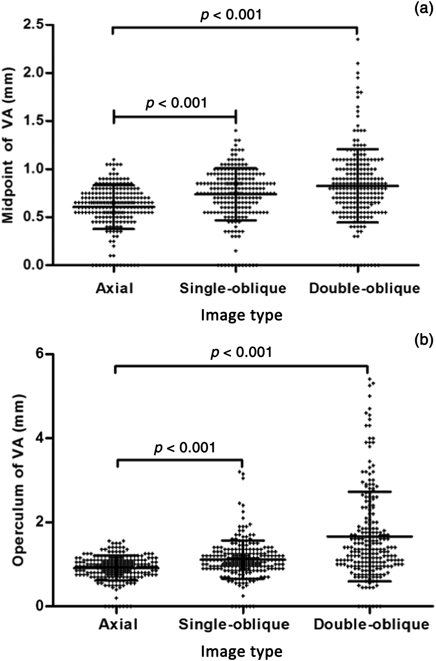
The vestibular aqueduct measurements for each image type are presented in Table 1, and Figures 5 and 6.
Box plots show the size of the (a) midpoint and (b) operculum measured in the axial, single-oblique and double-oblique images. The boundaries of the box plots indicate the 25th and 75th percentiles, and the whiskers indicate the minimum and maximum (range) of all values. The line within each box indicates the median. Vestibular aqueduct size was compared between the two groups using the Mann–Whitney U test with Bonferroni correction. VA = vestibular aqueduct

Scatter dot plot for the size of the (a) midpoint and (b) operculum of 224 ears measured in the axial, single-oblique and double-oblique images. The middle line within each cluster of dots indicates the mean. The lines above and below indicate the mean ± standard deviation. ‘+’ indicates the value of the size of the (a) midpoint and (b) operculum. Vestibular aqueduct size was compared between the two groups using the Mann–Whitney U test with Bonferroni correction. VA = vestibular aqueduct

Vestibular aqueduct size at midpoint and operculum, on axial, single-oblique and double-oblique images*

Data represent the mean ± the standard deviation (and range), in millimetres. *Total of 224 ears
A significant difference was identified in the size of the vestibular aqueduct as measured at the midpoint among the axial, single-oblique and double-oblique images (Kruskal–Wallis test). Post-hoc pairwise comparisons revealed statistically significant differences between the image types. Moreover, a significant difference in the size of the vestibular aqueduct as measured at the operculum was noted among the three image types. Post-hoc pairwise comparisons reached statistical significance.
The co-efficients of variation for the measurements obtained on the three image types are provided in Table 2. The co-efficients of variation were largest for the midpoint and operculum measurements obtained on the double-oblique images.
Co-efficients of variation for measurements obtained on each image type

Data presented in percentages
There was substantial agreement between the two radiologists for the midpoint measurements obtained using axial, single-oblique and double-oblique images (Table 3). The two readers had almost perfect agreement for the operculum measurements obtained using axial, single-oblique and double-oblique images (Table 3). The high inter-observer agreement for the midpoint and operculum measurements obtained on all image types implies good reproducibility.
Intraclass correlation co-efficients for vestibular aqueduct measurements, for each image type

Data in parentheses are the 95 per cent confidence intervals
Table 4 summarises the vestibular aqueducts according to morphological type in the axial, single-oblique and double-oblique images. None of the aqueducts appeared funnel-shaped on the axial images.
Numbers of vestibular aqueducts of each morphological type, on axial, single-oblique and double-oblique images

Statistically significant differences in the morphological types were observed among the axial, single-oblique and double-oblique images (p < 0.001). Further analyses revealed that the morphological types differed significantly between the axial and single-oblique images (p = 0.006), between the axial and double-oblique images (p < 0.001), and the between single-oblique and double-oblique images (p < 0.001).
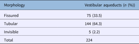
Examinations of the gross morphology on the CT images showed that tubular morphology was the most prevalent (144 out of 224; 64.3 per cent), followed by the fissured (75 out of 224; 33.5 per cent) and invisible (5 out of 224; 2.2 per cent) morphologies (Table 5).
Numbers of vestibular aqueducts according to gross morphology on CT images

CT = computed tomography
Discussion
The present study demonstrated that the morphology and dimensions of the vestibular aqueduct vary greatly depending on whether the evaluations are performed using axial, single-oblique or double-oblique images.
In an adult, the vestibular aqueduct has an inverted ‘J’ appearance, with a short ascending proximal segment and a longer distal descending segment. The proximal segment arises from the medial wall of the vestibule, and curves superiorly and medially into a bend, which is the narrowest portion of the aqueduct; this segment is called the isthmus and it corresponds to the bend. The distal straight segment enlarges along its inferior and posterior course, and ends as the external aperture on the posterior surface of the petrous pyramid.Reference Swartz6, Reference Ozgen, Cunnane, Caruso and Curtin15, Reference Pyle19 The isthmus is the narrowest segment of the aqueduct, measuring 0.3 mm in diameter.Reference Minerva, Mafee, Valvassori and Becker14 The outer aperture of the aqueduct measures approximately 2.0–6.0 mm in the larger diameter and 1.0 mm in the shorter diameter.Reference Minerva, Mafee, Valvassori and Becker14
Here, the size of the operculum was largest when measured on double-oblique images (1.66 ± 1.07 mm), followed by single-oblique (1.11 ± 0.45 mm) and axial (0.91 ± 0.30 mm) images (Table 1). This finding is in agreement with results reported previously.Reference Minerva, Mafee, Valvassori and Becker14 Lo et al. reported that seeing the entire endolymphatic sac on a single section requires double-oblique reformation at 70° from the infraorbital-meatal plane and 45° from the sagittal plane.Reference Lo, Daniels, Chakeres, Linthicum, Ulmer and Mark20 Because of the oblique orientation of the aqueduct, axial, coronal and sagittal images are differently angulated from its long axis. Single-oblique images are partially consistent with its oblique orientation. However, double-oblique images are completely consistent with its oblique orientation. Thus, double-oblique images show more of the vestibular aqueduct on a single section than do axial images. This explains why the size of the operculum was largest when measured on double-oblique images.
In the current study, the vestibular aqueduct measurements varied the most when using double-oblique images, but had little variability when using axial images. Our results showed that the SDs for both the midpoint and operculum measurements were largest when using double-oblique images (0.38 and 1.07, respectively), followed by single-oblique (0.27 and 0.45, respectively) and axial (0.23 and 0.30, respectively) images. A large SD indicates that the data points are far from the mean, while a small SD indicates that they are clustered closely around the mean. Indeed, the co-efficients of variation for the midpoint and operculum measurements were largest for the double-oblique images (47.5 per cent and 64.5 per cent, respectively). These findings confirm high variance in the size of the vestibular aqueduct when measured on double-oblique images, while the vestibular aqueduct measurements on axial and single-oblique images have low variance.
In terms of the morphology of the aqueduct, we found that the tubular form was the most prevalent (64.3 per cent), followed by the fissured (33.5 per cent) and invisible (2.2 per cent) forms. Moreover, the prevalence of each morphological type differed depending on whether axial, single-oblique or double-oblique images were utilised. In total, 75 ears (33.5 per cent) had a fissured aqueduct and 144 ears (64.3 per cent) had a tubular aqueduct in our study (Table 5). We considered the vestibular aqueduct to be fissured if it was funnel-shaped in any one of the axial, single-oblique or double-oblique images, but tubular in the other two image types. In fact, the fissured morphology is in agreement with the three-dimensional anatomy of the aqueduct. However, as mentioned above, the tubular morphology was the most prevalent, and this high prevalence may be related to our categorisation.
In addition, most of the vestibular aqueducts were found to be tubular on axial images. This is likely because the plane of axial images is inconsistent with the axis of the vestibular aqueduct. When the plane of the CT image is consistent with the axis of the vestibular aqueduct, then the vestibular aqueduct will usually appear as funnel-shaped in morphology.
Several limitations of our study should be noted. First, we did not examine whether age had an effect on or was related to the vestibular aqueduct measurements. However, prior studies by Vijayasekaran et al.Reference Vijayasekaran, Halsted, Boston, Meinzen-Derr, Bardo and Greinwald17 and Legeais et al.Reference Legeais, Haguenoer, Cottier and Sirinelli21 reported that the size of the vestibular aqueduct was unrelated to age. Thus, it is unlikely that age affected our findings. Second, it was difficult to demonstrate the fissured morphology on single-oblique and double-oblique images, particularly as we positioned the reference lines through the midpoint of the vestibular aqueduct; hence, the proximal segment of the vestibular aqueduct was non-linear. This may have resulted in an underestimation of the prevalence of the fissured morphology in our subject population. Finally, our study lacked anatomical measurements of the vestibular aqueduct. However, we can suppose that axial measurements of the aqueduct on axial CT images should be slightly larger than the anatomical measurements, as axial images are significantly angulated from the axis of the aqueduct.
• An enlarged vestibular aqueduct is a common imaging abnormality in computed tomography evaluations of children with sensorineural hearing loss
• The vestibular aqueduct diameter at the post-isthmic segment midpoint on axial images is a potential diagnostic standard for an enlarged vestibular aqueduct
• Because of the oblique orientation of the vestibular aqueduct, axial, coronal and sagittal images are differently angulated from its long axis
• Single-oblique images are partially consistent with its oblique orientation, but double-oblique images are completely consistent
• The vestibular aqueduct morphology and dimensions were highly variable among axial, single-oblique and double-oblique images
• Regarding aqueduct morphology, the tubular form was most prevalent (64.3 per cent), followed by fissured (33.5 per cent) and invisible (2.2 per cent) forms
Conclusion
Our results revealed high variability in the morphology and dimensions of the vestibular aqueduct among axial, single-oblique and double-oblique images.
Competing interests
None declared