1. Introduction
Combustion chambers in many propulsion systems such as diesel engines, gas turbine engines and rocket engines operate at high-pressure (high- $p$) conditions. In those engines, the pressure is above critical pressures of several species, and the combustion gas may become a fluid mixture of species at supercritical pressure. The interaction of this fluid with the combustion chamber wall is the aspect stimulating the subject of this study. Indeed, heat transfer near the wall, in the boundary layer, strongly affects the processes inside the combustion chamber through quenching reactions and soot formation. Thus, understanding the physics of the boundary layer is crucial for the thermal design of many propulsion systems.
Considering that combustion chamber walls are generally cooled, boundary layers have a large temperature gradient in the wall-normal direction. This large temperature gradient leads to variations in thermodynamic properties and molecular transport properties. For high- $p$ situations, these property variations deviate from the perfect-gas law due to real fluid effects, and, thus, flow physics of the boundary layer is different from that under atmospheric-
 $p$ conditions. In addition, at high-
 $p$, thermal diffusion becomes important (Harstad & Bellan Reference Harstad and Bellan2000) so that even for binary species mixing the diffusive species-mass flux is not simply given by the Fick's law (Harstad & Bellan Reference Harstad and Bellan2004). These additional diffusion aspects make the flow physics more complicated.
To investigate the flow physics of boundary layers at high- $p$ conditions, direct numerical simulation (DNS) is an attractive method. This is because DNS provides detailed turbulent statistics and an opportunity to explore flow structures since it numerically resolves turbulent motions at all scales overwhelmingly responsible for the dissipation. In the past, Bae, Yoo & Choi (Reference Bae, Yoo and Choi2005) and Bae, Yoo & McEligot (Reference Bae, Yoo and McEligot2008) used DNS to simulate heated
 $\mathrm {CO}_{2}$ turbulent vertical pipe and annular flows with buoyancy effects at small Mach numbers. In those studies, it was found that due to buoyancy effects, unique velocity profiles cause a decrease in turbulent heat fluxes. Nemati et al. (Reference Nemati, Patel, Boersma and Pecnik2015, Reference Nemati, Patel, Boersma and Pecnik2016) and Peeters et al. (Reference Peeters, Pecnik, Rohde, van der Hagen and Boersma2016) also simulated vertical pipe and annular flows at small Mach numbers. The results from those investigations revealed that turbulent statistics and turbulent structures are significantly affected by variations in dynamic viscosity and density. More recently, Kawai (Reference Kawai2019) used a fully compressible DNS to simulate heated boundary layers of supercritical hydrogen over zero-pressure-gradient flat plates, and reported that real fluid effects at transcritical conditions cause strong density fluctuations, and that the strong density fluctuations alter turbulent statistics from those of incompressible constant-property flow. Ma, Yang & Ihme (Reference Ma, Yang and Ihme2018) used fully compressible DNS to study a planar turbulent channel flow of supercritical nitrogen and demonstrated that semilocal scaling has limited success near a wall where violent fluctuations are found. Toki, Teramoto & Okamoto (Reference Toki, Teramoto and Okamoto2020) also simulated a planar turbulent channel flow of supercritical nitrogen and introduced a new transformation equation for the temperature profile in the logarithmic region. Transcritical channel flow of R-134a was simulated by Kim, Hickey & Scalo (Reference Kim, Hickey and Scalo2019) and it was reported that even the recent improvements to the scaling laws cannot accurately capture the velocity distribution in that transcritical flow.
These previous DNS studies have mainly focused on effects of variations in thermodynamic properties and molecular transport properties in single-species boundary layers. They have revealed the physics of single-species boundary layers at high- $p$ conditions, however, there are no equivalent studies for boundary layers where the fluid is composed of more than one species. The present study begins to fill the gap of understanding high-
 $p$ multi-species boundary layers by initiating the study of this topic with a binary-species fluid and examining how the results differ from, or are similar to, the single-species situation. Because the previous relevant studies have not addressed this topic, this investigation focuses on the species-mass diffusion in the high-
 $p$ boundary layers.
This paper is organized as follows. In § 2 we recall the governing equations consisting of the conservation equations and the equation of state; details are relegated to Appendices A and B. The numerical methods are briefly described in § 3. The configuration, boundary conditions and initial conditions are summarized in § 4. The results, presented in § 5, encompass flow statistics and flow structures, with emphasis on species-mass diffusion for the binary-species simulations. Flow statistics are presented in § 5.2. Flow structures for the binary-species case are investigated in § 5.3. Species-mass diffusion in the binary-species cases is discussed in § 5.4. Finally, conclusions are offered in § 6.
2. Governing equations
The governing equations are the conservation equations complemented by the equation of state (EOS).
2.1. Differential conservation equations
The conservation equations for multi-species flow (Okong'o & Bellan Reference Okong'o and Bellan2002) are
 $$\begin{gather} \frac{\partial\rho}{\partial t}+\frac{\partial}{\partial x_{j}}[ \rho u_{j}] =0, \end{gather}$$
 $$\begin{gather}\frac{\partial}{\partial t}\left( \rho u_{i}\right) +\frac{\partial }{\partial x_{j}}[ \rho u_{i}u_{j}+p\delta_{ij}-\sigma_{ij}] =0, \end{gather}$$
 $$\begin{gather}\frac{\partial}{\partial t}\left( \rho e_{t}\right) +\frac{\partial }{\partial x_{j}}[ ( \rho e_{t}+p) u_{j}-u_{i}\sigma _{ij}+q_{j}] =0, \end{gather}$$
 $$\begin{gather}\frac{\partial}{\partial t}\left( \rho Y_{\alpha}\right) +\frac{\partial }{\partial x_{j}}[ \rho Y_{\alpha}\ u_{j}+J_{\alpha j}] =0, \end{gather}$$
where  $\alpha \in \lbrack 1,N-1]$,
 $t$ denotes the time,
 $x$ is a Cartesian coordinate,
 $u$ is the velocity,
 $e_{t}=e+u_{i}u_{i}/2$ is the total energy (i.e. internal energy,
 $e$, plus kinetic energy),
 $Y_{\alpha }$ is the mass fraction of species
 $\alpha$,
 $N$ is the number of species,
 $\boldsymbol {q}$ is the heat flux and
 $\boldsymbol {J}_{\alpha }$ is
 $\alpha$-species mass flux. The subscripts
 $i$ and
 $j$ refer to spatial coordinates. The Newtonian viscous stress tensor
 $\sigma _{ij}$ is written as
 \begin{equation} \sigma_{ij}=\mu\left( 2S_{ij}-\dfrac{2}{3}S_{kk}\delta_{ij}\right) ,\quad S_{ij}=\dfrac{1}{2}\left( \dfrac{\partial u_{i}}{\partial x_{j}} +\dfrac{\partial u_{j}}{\partial x_{i}}\right) , \end{equation}
where  $\mu$ is the viscosity and
 $S_{ij}$ is the strain-rate tensor.
Because of the different constitutive relations used for expressing  $\boldsymbol {J}_{\alpha }$ and
 $\boldsymbol {q}$, (2.1)–(2.4) under high-
 $p$ conditions have ultimately a different form from that used under atmospheric-
 $p$ conditions. The present
 $\boldsymbol {J}_{\alpha }$ and
 $\boldsymbol {q}$ expressions are based on the full matrices of mass diffusion coefficients and thermal-diffusion factors derived by Harstad & Bellan (Reference Harstad and Bellan2004). Since (2.1) is solved, only a set of independent (
 $N-1)$ species equations rather than the set of
 $N$ dependent species is considered; in these (
 $N-1)$ equations, the original molar-fraction fluxes and the heat flux were rewritten to account for only (
 $N-1)$ gradients. The final form is
 $$\begin{gather} \boldsymbol{J}_{\alpha}={-}\rho\left[ Y_{\alpha}\left( D_{T,\alpha}\right) \frac{\boldsymbol{\nabla} T}{T}+Y_{\alpha}\left( D_{p,\alpha}\right) \frac{\boldsymbol{\nabla} p} {p}+\sum_{\beta=1}^{N-1}\left(D_{\alpha\beta}^{\prime} \frac{m_{\alpha} }{m_{\beta}}\right) \boldsymbol{\nabla} Y_{\beta}\right] , \end{gather}$$
 $$\begin{gather}\boldsymbol{q}={-}\lambda\boldsymbol{\nabla} T+\sum_{\alpha=1}^{N-1}\boldsymbol{J}_{\alpha}\left[ \left( \frac{h_{\alpha}}{m_{\alpha}}-\frac{h_{N}}{m_{N}}\right) -R_{u}T\left( \frac{\bar{\alpha}_{T,\alpha}^{b}}{m_{\alpha}}-\frac {\bar{\alpha}_{T,N}^{b}}{m_{N}}\right) \right] , \end{gather}$$
where
 $$\begin{gather} D_{T,\alpha}={-}\sum_{\beta=1}^{N}\bar{\alpha}_{T,\beta}^{b}\mathbb{D} _{\beta\alpha},\quad{}D_{p,\alpha}=\frac{p}{R_{u}T}\sum _{\beta=1}^{N}v_{\beta}\mathbb{D}_{\beta\alpha}, \end{gather}$$
 $$\begin{gather}D_{\alpha\gamma}=\sum_{\beta=1}^{N}\mathbb{D}_{\alpha\beta}\alpha _{D\beta\gamma}, \end{gather}$$
 $$\begin{gather}\bar{\alpha}_{T,\alpha}^{b}=\sum_{\beta=1}^{N}X_{\beta}\alpha_{T,\beta\alpha }^{b}, \end{gather}$$
 $$\begin{gather}D_{\alpha\beta}^{\prime}=D_{\alpha\beta}-\left( 1-\frac{m_{\beta}}{m_{N} }\right) \left( \sum_{\gamma=1}^{N-1}D_{\alpha\gamma}X_{\gamma}\right) . \end{gather}$$
Here,  $T$ is the temperature;
 $X_{\alpha }=Y_{\alpha }m/m_{\alpha }$ is the molar fraction;
 $m_{\alpha }$ is the species molar mass;
 $m$ is the mixture molar mass,
 $m=\sum _{\gamma =1}^{N}m_{\gamma }X_{\gamma };$
 $v_{\alpha }=(\partial v/\partial X_{\alpha })_{T,p,X_{\beta }(\beta \neq \alpha )}$ is the partial molar volume, where the molar volume is
 $v=1/n$ and
 $n=\rho /m$ is the molar density;
 $h_{\alpha }=(\partial h/\partial X_{\alpha })_{T,p,X_{\beta }(\beta \neq \alpha )}$ is the partial molar enthalpy, where the molar enthalpy is
 $h=G-T(\partial G/\partial T)_{p,X}$ with
 $G$ being the Gibbs energy
 $;$
 $R_{u}$ is the universal gas constant;
 $D_{\alpha \gamma }$ are the pairwise mass diffusion coefficients;
 $\alpha _{T,\alpha \beta }^{b}$ are the binary thermal-diffusion factors; and
 $\lambda$ is the thermal conductivity. The mass diffusion factors,
 $\alpha _{D\alpha \beta },$ are calculated from thermodynamics as
 \begin{equation} \alpha_{D\alpha\beta}\equiv\dfrac{1}{R_{u}T}X_{\alpha}\dfrac{\partial \mu_{\alpha}}{\partial X_{\beta}}=(\delta_{\alpha\beta}-\delta_{\alpha N})+X_{\alpha}(R_{\alpha\beta}-R_{\alpha N}), \end{equation}
with  $1\leqslant \alpha \leqslant N$,
 $1\leqslant \beta \leqslant N-1$, and
 \begin{equation} R_{\alpha\beta}\equiv\frac{\partial\ln\gamma_{\alpha}}{\partial X_{\beta}}, \end{equation}
with  $1\leqslant \alpha \leqslant N,\text { }1\leqslant \beta \leqslant N$. In (2.12) and (2.13),
 $\mu _{\alpha }$ is the chemical potential of species
 $\alpha$ written in terms of
 $N-1$ species;
 $\gamma _{\alpha }\equiv \varphi _{\alpha }/\varphi _{\alpha }^{o}$, where
 $\varphi$ is the fugacity coefficient written in terms of
 $N$ species and the superscript
 $o$ denotes the pure (
 $X_{\alpha }=1)$ limit. More details are provided in Appendix A.
2.2. Equation of state
Equations (2.1)–(2.4) are coupled with a modified Peng–Robinson (PR) EOS introduced by Harstad, Miller & Bellan (Reference Harstad, Miller and Bellan1997),
 \begin{equation} p=\dfrac{R_{u}T\left(\displaystyle\sum_{\alpha=1}^{\alpha=N}X_{\alpha}\right) }{\left( v_{PR}-b_{mix}\right) }-\dfrac{a_{mix}}{\left( v_{PR}^{2}+2b_{mix} v_{PR}-b_{mix}^{2}\right) }. \end{equation}
Here,  $v_{PR}$ is the molar PR volume and
 $v=v_{PR}+v_{s}$, where
 $v_{s}$ is the volume shift introduced for improving the accuracy of the PR EOS at high pressure, the
 $v_{s}$ computation was described in detail elsewhere (Okong'o, Harstad & Bellan Reference Okong'o, Harstad and Bellan2002). The calculation of
 $a_{mix}$ and
 $b_{mix}$ together with other details are provided in Appendix B.
3. Numerical method
The differential equations combined with the EOS described in § 2 are numerically solved using a fourth-order explicit Runge–Kutta time integration and a sixth-order compact scheme spatial discretization (Lele Reference Lele1992). The conservation equations are first solved, and  $T$ and
 $p$ are obtained as an iterative solution which satisfies both values of
 $\rho$ and
 $e$, as obtained from the conservation equations. In order to ensure time stability, the conservative variables were filtered using the eighth-order compact filter described elsewhere (Gaitonde & Visbal Reference Gaitonde and Visbal1998). Because the order of the filter is larger than that of the discretization, no physical information is removed by the filter which only serves to remove unphysical fluctuations associated with long computer run times. In the past (Sciacovelli & Bellan Reference Sciacovelli and Bellan2019), a parametric study using several filter coefficients (0.45, 0.475 and 0.49) was conducted indicating that the value 0.49 was sufficiently large to ensure that the filter only acts on the shortest wavelengths that can be resolved on the grid and it does not affect the physical content of the data. The code was parallelized using three-dimensional domain decomposition and message passing. The tridiagonal solvers for the compact derivative scheme and the compact filter were efficiently parallelized using a well-established method (Muller & Scheerer Reference Muller and Scheerer1991).
4. Configuration, boundary conditions and initial conditions
Currently, there are two approaches which may lead to well-converged statistics in boundary layer simulations: (1) using spatial boundary layers with known turbulent inlet boundary conditions, and (2) employing the recycling method in which turbulent velocities on a specified plane are rescaled and recycled back to the inlet as the inflow boundary condition. However, simulating spatial boundary layers would be very computationally intensive for the present situation because here the modified PR EOS is solved using an iteration method and the transport properties are computed at each time step as a function of the local pressure, temperature and composition, all of which requires a large computation time. Furthermore, the recycling method is not applicable because there is no data regarding the self-similarity of mass fraction profiles.
Therefore, the choice of the present configuration is that of a temporal boundary layer, an approach which is justified by the realization that temporal boundary layers and spatial boundary layers have the same physics (e.g. Martín Reference Martín2004; Kozul, Chung & Monty Reference Kozul, Chung and Monty2016). To be consistent with boundary layer notations in the literature,  $(x_{1},x_{2},x_{3})\equiv (x, y, z)$ denote the streamwise, wall-normal and spanwise directions and
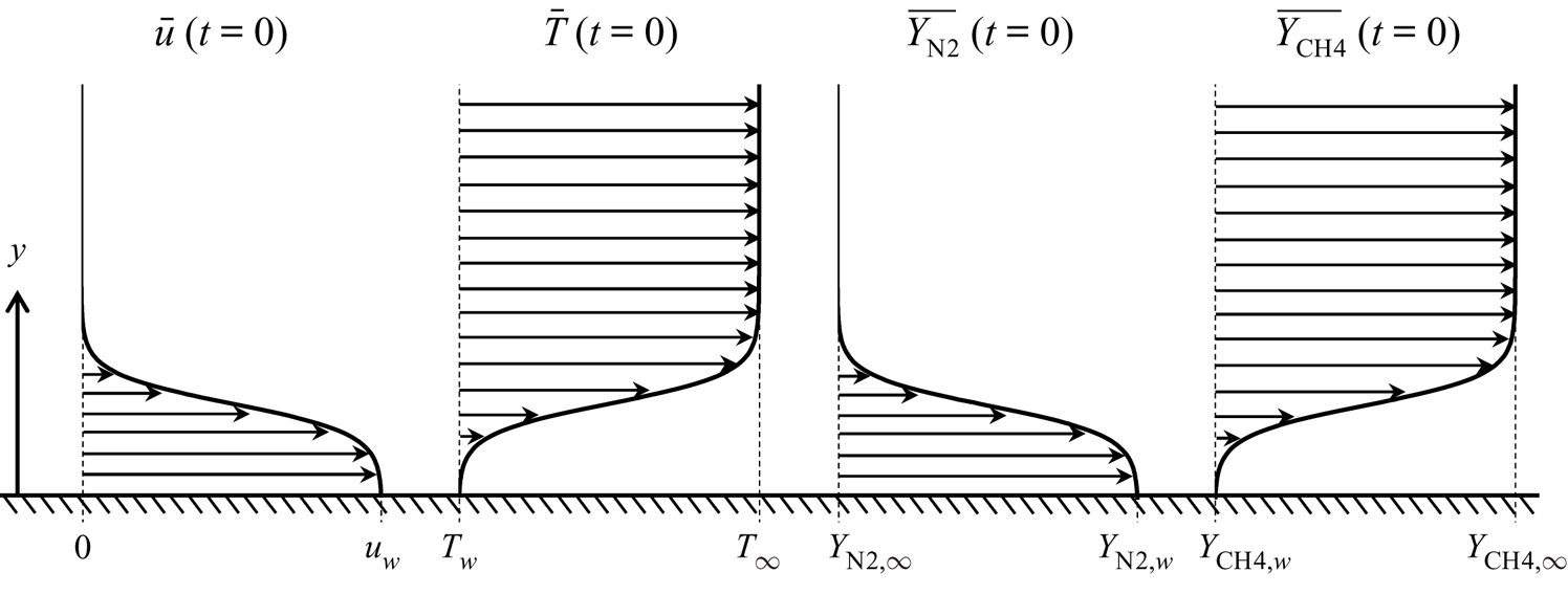
 $(u_{1} ,u_{2},u_{3})\equiv (u,v,w)$. For single-species cases, the working fluid is nitrogen and for binary-species cases the working fluid is a mixture of nitrogen and methane. Figure 1 provides a sketch of the configuration. The wall moves at constant velocity, while the far field is at rest. Periodic boundary conditions are applied to the streamwise (
 $x$) and spanwise (
 $z$) directions. No-slip wall conditions are applied at the wall, and the temperature and velocity are there constant in space and time. The simulation is initiated with a thin shear layer, and continues until the flow field reaches a target Reynolds number. In the past, the same configuration was used by Kozul et al. (Reference Kozul, Chung and Monty2016) to conduct DNS of an incompressible boundary layer, and it was shown that turbulent statistics of the temporal set-up agree very well with those of spatial boundary layers. In contrast to Kozul et al. (Reference Kozul, Chung and Monty2016), the upper-domain boundary condition consists of non-reflecting boundary conditions (Okong'o & Bellan Reference Okong'o and Bellan2002); the mass flux of each species is set to be null at a wall.
Sketch of initial profiles of mean streamwise velocity, temperature and mass fractions.

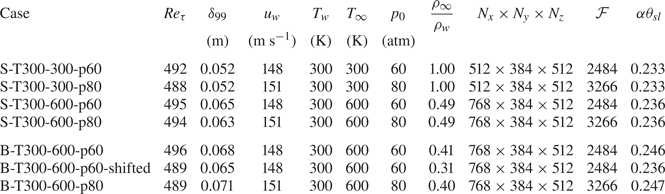
The simulations encompass four single-species cases and three binary-species cases, all listed in table 1. Each case is denoted by an acronym is which the first character indicates the single-species ( $S$) or binary-species case (
 $B$). The adopted notation is that subscripts
 $w$ and
 $\infty$ indicate wall and far field locations, respectively. In table 1,
 $Re_{\tau }\equiv u_{\tau }\delta _{99}\rho _{w}/\mu _{w}$ is the friction Reynolds number where
 $\delta _{99}$ is a length which is 99 % of boundary layer thickness,
 $u_{\tau }\equiv \sqrt {\tau _{w}/\rho _{w}}$, where
 $\tau _{w}$ is the fluid shear stress at the wall and
 $\rho _{w}$ is the fluid density at the wall. Table 1 lists the friction Reynolds numbers at the time when the data shown in and thereafter § 5.2 are obtained. In all simulations the Mach number,
 $Ma$, value associated with the wall velocity
 $u_{w}$ is 0.4, based on the sound speed of pure nitrogen. Although the
 $Ma$ value is modest in the realm of compressible flows, due to the strong nonlinearity of the EOS, the flow cannot be considered incompressible. Indeed, for a real-gas EOS, pressure gradients are much larger than in atmospheric flows at otherwise same conditions because small spatial changes in temperature and composition induce large changes in pressure as a result of the strong nonlinearity. The wall temperature
 $T_{w}$ is 300 K in all cases. The far field temperature
 $T_{\infty }$ is either 300 K (S-T300-300-p60 and S-T300-300-p80) or 600 K. The temperature difference between
 $T_{w}$ and
 $T_{\infty }$ causes variations in thermodynamic and molecular transport properties. The initial pressure
 $p_{0}$ is 60 or 80 atm, both values being above the critical pressures of nitrogen and methane. The gradients of temperature and mass fraction induce density variation and
 $\rho _{\infty } /\rho _{w}$ is the density ratio between the wall fluid and the far field fluid. Table 2 lists the critical properties of the species and provides information regarding their thermodynamic regime at the initial conditions.
List of computational cases and conditions. All symbols are defined in the text.

Species thermodynamic critical properties,  $T_c$ and
 $p_c$, and reduced properties,
 $T_r$ =
 $T/T_c$ and
 $p_r$ =
 $p/p_c$.

In table 1  $N_{x}$,
 $N_{y}$ and
 $N_{z}$ are the number of grid points in each direction;
 $\mathcal {F}$ is a scaling factor defined elsewhere (Masi et al. Reference Masi, Bellan, Harstad and Okong'o2013; Sciacovelli & Bellan Reference Sciacovelli and Bellan2019) representing the scaling of the viscosity by a reference value in order to ensure that the Reynolds number value is such that DNS is feasible. Then, all transport properties are scaled by
 $\mathcal {F}$, in particular ensuring that the Schmidt number and Prandtl number have physical values. The momentum thickness of the layer is
 $\theta _{sl}$ (discussed in § 4.1),
 $\alpha$ is a real number (see Appendix C) and
 $\alpha \theta _{sl}$ is a parameter used to derive perturbations of the initial flow; details are provided in Appendix C.
4.1. Initial profiles
Typically, boundary layer simulations are conducted considering a flow of a single chemical species. However, in the present simulations the emphasis is on the binary-species mixing and the differences from the single-species situation. Since the velocity field is affected by species mixing, the growth rate of perturbations is consequently affected by mixing. Thus, here the adopted initialization is found employing the procedure used in previous mixing layer simulations of Masi et al. (Reference Masi, Bellan, Harstad and Okong'o2013) and Sciacovelli & Bellan (Reference Sciacovelli and Bellan2019). The initial profiles are composed of mean quantities upon which perturbations are imposed. The mean profiles are based on tangent hyperbolic functions, and the perturbations are analytically derived (shown in Appendix D). The mean profiles of velocities, temperature and pressure are set to resemble a shear layer as
 $$\begin{gather} \bar{u}(y) =u_{w}-\frac{1}{2}u_{w}\left( 1-\tanh\left[ \frac {D}{2\theta_{sl}}\left( 1-\frac{y}{D}\right) \right] \right) , \end{gather}$$
 $$\begin{gather}\bar{T}(y) =T_{w}+\frac{1}{2}\left( T_{\infty}-T_{w}\right) \left( 1-\tanh\left[ \frac{D}{2\theta_{sl}}\left( 1-\frac{y}{D}\right) \right] \right) , \end{gather}$$
 $$\begin{gather}p =p_{0},\quad v=0,\quad w=0, \end{gather}$$
where  $D$ is the displacement thickness. The overline
 $\overline {(\cdot )}$ indicates averaging in the homogeneous (
 $x,z)$ plane. The displacement thickness
 $D$ is set to
 $Re_{D}\equiv Du_{w}/\nu _{w}=1000$ (
 $\nu _{w}\equiv \mu _{w}/\rho _{w}$), consistent with Kozul et al. (Reference Kozul, Chung and Monty2016) who did a parametric study of the initial profile based on
 $Re_{D}$, and demonstrated that in those cases
 $Re_{D}=1000$ results in a natural turbulent evolution as soon as the computation was initiated. In the present study the momentum thickness
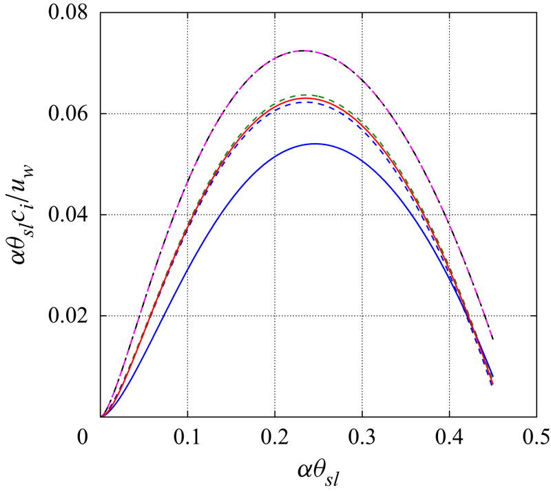
 $\theta _{sl}$ is specified by stability analyses to achieve the largest growth rate for the initial perturbations. The numerical methods of the stability analyses yielding the perturbations are provided in Appendix C.
In the binary-species cases, mean profiles of mass fractions are set as
 $$\begin{gather} \overline{Y_{\textrm{CH}4}}(y) =1+\frac{1}{2}\left( 1-\tanh\left[ \frac{D_{mass} }{2\theta_{sl}}\left( 1-\frac{y}{D_{mass}}\right) \right] \right) , \end{gather}$$
 $$\begin{gather}\overline{Y_{\textrm{N}2}}(y) =1-\overline{Y_{\textrm{CH}4}}(y), \end{gather}$$
where  $D_{mass}$ is a parameter determining the inflection point of the profiles. The parameter is set to
 $D_{mass}=D$ in B-T300-600-p60 and B-T300-600-p80, and, thus, initial profiles of mass fractions are similar to those of velocity and temperature. The parameter is set to
 $D_{mass}=8D$ in B-T300-600-p60-shifted to promote strong mixing away from the wall.
4.2. Domain size and grid spacing
The domain size is determined by a specified boundary layer thickness,  $\delta _{p}$. The specified friction Reynolds number is 500 so as to be comparable to the spatial boundary layer of Schlatter & Örlü (Reference Schlatter and Örlü2010) for which
 $Re_{\tau }=492$. When the friction Reynolds number is 500,
 $\delta _{p}\simeq 0.07\ \textrm {m}$, which is the value adopted here. The wall-normal domain size is set to
 $L_{y}=3\delta _{p}$. The streamwise domain size is set to
 $L_{x}=2{\rm \pi} \delta _{p}$, and the spanwise domain size is set to
 $L_{z}={\rm \pi} \delta _{p}$. This domain size was proved to be sufficiently large to capture the main dynamic features of the flow and the wall-normal statistics (Kozul et al. Reference Kozul, Chung and Monty2016). The grid spacing is uniform in the streamwise and spanwise directions. The grid spacing in the wall-normal direction is determined by the following tangent hyperbolic function:
 \begin{equation} y_{j}=\frac{L_{y}}{\alpha_{st}}\tanh\left[{-}1+\frac{j-1}{N_{y}-1}\tanh ^{{-}1}(\alpha_{st})\right]. \end{equation}
Here  $\alpha _{st}$ is a constant value,
 $\alpha _{st}=0.985$. The wall-normal coordinates based on wall units are defined as
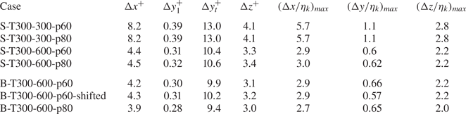
 $y^{+}\equiv yu_{\tau }/\nu _{w}$. The grid resolutions in wall units are shown in table 3. They are evaluated as
 $\Delta x_{i}^{+}\equiv \Delta x_{i}u_{\tau }/\nu _{w}$, where
 $\Delta x_{i}$ is the grid spacing in the
 $x_{i}$ direction;
 $\Delta x^{+}$ and
 $\Delta z^{+}$ are grid resolutions in the streamwise and spanwise directions, respectively. The wall-normal grid spacings
 $\Delta y_{t}^{+}$ and
 $\Delta y_{1}^{+}$ correspond to those at the top and bottom of the domain. For each simulation, the grid resolution listed in table 1 is that at the time when
 $Re_{\tau} \approx 500$. In addition, table 3 lists the maximum grid spacing in terms of the Kolmogorov scale
 $\eta _{k}$ calculated as
 \begin{equation} \eta_{k}=\left( \frac{\left( \bar{\mu}\right) ^{3}}{\left( \bar{\rho}\right) ^{2}\varepsilon}\right) ^{1/4}, \end{equation}
where  $\varepsilon \equiv \overline {\sigma _{ij}^{\prime }\partial u_{i}^{\prime }/\partial x_{j}}$ is the turbulent kinetic energy (TKE) dissipation. The notation
 $(\cdot )^{\prime }$ indicates fluctuation from the average. The Kolmogorov scale is commonly quoted as the smallest scale that must be resolved in DNS, however according to Moin & Mahesh (Reference Moin and Mahesh1998), this requirement is too stringent. Moin & Mahesh (Reference Moin and Mahesh1998) convincingly show that for several configurations, including boundary layers, the smallest required resolved scale must only be
 $O(\eta )$, not equal to
 $\eta$. Prior DNS studies have reported the resolution requirements of
 $\Delta x<12\min \{\eta _{k},\eta _{\theta }\},\Delta y<2\min \{\eta _{k},\eta _{\theta }\},\Delta z<6\min \{\eta _{k},\eta _{\theta }\}$, where
 $\eta _{\theta }\equiv \eta _{k}\sqrt {1/Pr}$ is the Bachelor scale (Zonta, Marchioli & Soldati Reference Zonta, Marchioli and Soldati2012; Lee et al. Reference Lee, Jung, Sung and Zaki2013; Patel, Boersma & Pecnik Reference Patel, Boersma and Pecnik2016; Kawai Reference Kawai2019). Table 3 shows that the present grid resolutions satisfy the requirements in terms of the Kolmogorov scale. Since the molecular Prandtl number
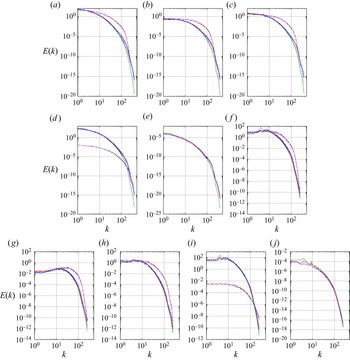
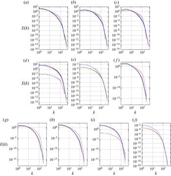
 $Pr$ is less than 1 in all cases, the requirements concerning the Batchelor scale are also satisfied. However, these requirements are insufficient for binary-species flows, because the Soret effect and the species-mass diffusion can affect the length scale of thermal diffusion (Masi et al. Reference Masi, Bellan, Harstad and Okong'o2013). Therefore, one-dimensional spectra of all quantities were investigated to check the grid resolutions (shown in Appendix E). The spectra show the smoothness associated with turbulent characteristics, and there is no accumulation of energy at the smallest scales, thereby indicating excellent resolution. Additionally, to check the validity of the chosen domain size, two-point correlations were computed (not shown) that compared very favourably with similar plots in the literature (e.g. Duan, Beekman & Martín Reference Duan, Beekman and Martín2010, Reference Duan, Beekman and Martín2011).
Grid resolution and maximum resolution normalized using the Kolmogorov scale  $\eta _{K}$.

5. Results
Temporal flows do not achieve a statistical steady state, however, they reach a self-similar state which is representative of the physical situation under consideration. To show that such a state is reached in the simulations, in § 5.1 it is shown that the simulations do reach a self-similar state and that the resolution during the flow evolution is appropriate, leading to the state at  $Re_{\tau }\approx 500$. Further, for each case in table 1, the state at
 $Re_{\tau }\approx 500$ is analysed. First, the mean flow field, turbulent fluctuations and TKE are addressed in § 5.2. Then in § 5.3 attention is turned to the instantaneous details of the flow by investigating the velocity, temperature and mass fraction spatial structure. Finally, the details of species-mass diffusion are examined in § 5.4 with special attention to the Soret effect.
5.1. Temporal evolution of the flow
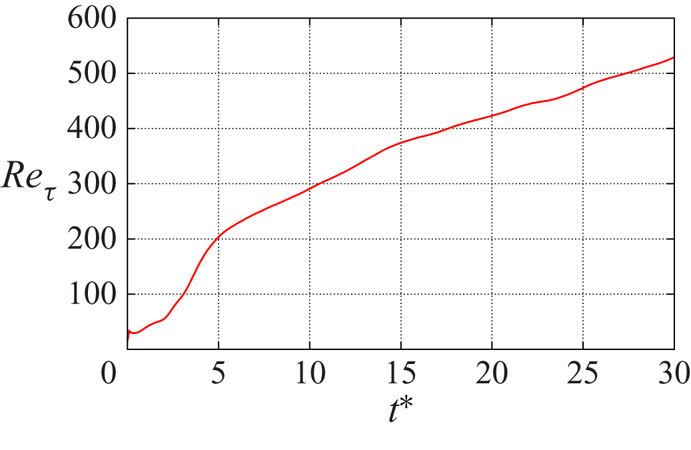
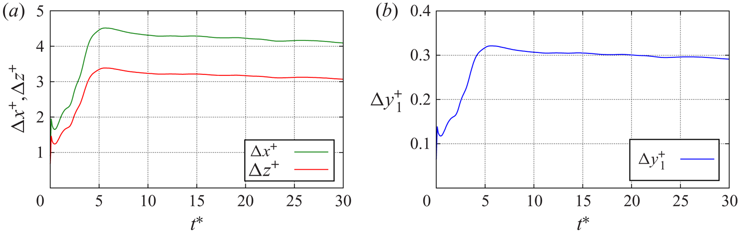
To understand the temporal evolution of the flow in the present configuration, figure 2 displays the time history of  $Re_{\tau }$ for B-T300-600-p60. The computational time is non-dimensionalized as
 $t^{\ast }\equiv tu_{w}/\delta _{p}$. The friction Reynolds number monotonically increases and reaches the specified value
 $Re_{\tau }=500$ at
 $t^{\ast }=27$. Furthermore, figure 2 shows that
 $Re_{\tau }$ increases drastically before
 $t^{\ast }=5$ but after
 $t^{\ast }=10$ it assumes a more subdued and quasi-uniform rate of increase, the latter attribute being symptomatic of reaching self-similarity at
 $Re_{\tau }=300$. Accordingly, figure 3 shows that the time-wise resolution variation tacks well this
 $Re_{\tau }$ growth history. In all directions, the grids reach a peak at
 $t^{\ast }=5$ and afterwards slightly decrease with
 $t^{\ast }$. However, the decrease in the grid resolution is very small in all directions and the values reached at
 $t^{\ast }=27$ corresponding to
 $Re_{\tau }=500$ are almost the same as their peak values at
 $t^{\ast }=5$. This information regarding grid history complements that shown in § 4.2 indicating that the grid resolution is sufficient before the attainment of
 $Re_{\tau }=500$ as it is also at that final state.
Time history of the friction Reynolds number in B-T300-600-p60.

Time histories of the grid resolutions in wall units in B-T300-600-p60: (a)  $\Delta x^{+}$ and
 $\Delta z^{+}$; (b)
 $\Delta y_{1}^{+}$.

This time history indicates that the flow field varies substantially before  $t^{\ast }=5$, whereas the variation becomes moderate after
 $Re_{\tau }=300$ at
 $t^{\ast }=10$. To further investigate the flow variation with
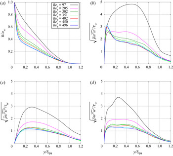
 $t^{\ast }$, in figure 4 the mean velocity and velocity fluctuations are compared at different
 $t^{\ast }$ values. The mean profiles and fluctuations are calculated by averaging in homogeneous
 $(x,z)$ planes;
 $\widetilde {( \cdot ) }$ indicates the Favre average and
 $(\cdot )^{\prime \prime }$ indicates fluctuations from the Favre average. The comparison shows that the differences among
 $Re_{\tau }=97$,
 $205$ and
 $302$ are large in all plots, whereas profiles at
 $Re_{\tau }=496$ agree well with those at
 $Re_{\tau }=402$ and
 $450$. Especially, the profiles at
 $Re_{\tau }=496$ collapse on those at
 $Re_{\tau }=450$. This observation indicates that a self-similarity appears in the mean velocity and velocity fluctuations after
 $Re_{\tau }=400$, a result which is somewhat more constraining in terms of the
 $Re_{\tau }$ value than that observed in figure 2. Thus, the flow has reached self-similarity at
 $Re_{\tau }=496$. All following analyses are conducted at the time when
 $Re_{\tau }\approx 500,$ and, thus, the flow fields are analysed at the state when the velocity field is self-similar.
Comparison of mean velocity and velocity fluctuations at the different computational time in B-T300-600-p60: (a) mean streamwise velocity, (b) streamwise velocity fluctuation, (c) wall-normal velocity fluctuation and (d) spanwise velocity fluctuation.

5.2. Flow statistics
The analysis first focuses on the most basic quantities in the flow such as mean profiles, fluctuations and the TKE budget. All analyses are conducted at the time when  $Re_{\tau }\approx 500$, as shown in table 1.
5.2.1. Mean flow field
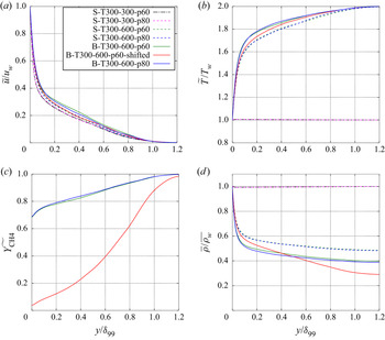
Mean profiles are calculated by averaging in the homogeneous  $(x,z)$ plane; the averages can be of regular type or Favre averages. Figure 5 shows non-dimensionalized mean profiles by the corresponding values at the wall –
 $\tilde {u}/u_{w},\tilde {T}/T_{w},\bar {\rho }/\rho _{w}$ – and
 $\widetilde {Y_{\textrm {CH}4}}$ for the binary-species cases. The qualitative characteristics of
 $\tilde {u}/u_{w}$ are the same in all cases in that the velocity monotonically decreases from the wall to the far field, with the gradient being much larger near the wall. The
 $\tilde {T}/T_{w}$ profile is almost the same in S-T300-300-p60 and S-T300-300-p80, because
 $T_{w}$ and
 $T_{\infty }$ have the same values in these cases. In the other cases,
 $\tilde {T}/T_{w}$ monotonically increases from the wall to the far field, and the gradient is much larger near the wall. Note that
 $\widetilde {Y_{\textrm {CH}4}}$ also monotonically increases from the wall to the far field, but there is no large gradient near the wall. The difference between the mass fraction profiles is a manifestation of the initial profile: the value at the wall is approximately 0.7 in B-T300-600-p60 and B-T300-600-p80, and this value is larger than that in B-T300-600-p60-shifted. Although the initial mass fraction of methane is almost 0 at the wall, and that at the far field is 1, the inflection point of the hyperbolic tangent function is shifted to a larger
 $y$ value in B-T300-600-p60-shifted. Therefore, it takes a longer time for methane to reach the wall in B-T300-600-p60-shifted, the gradient is larger and
 $\widetilde {Y_{\textrm {CH}4}}$ is smaller at the wall. The variation in
 $T$ and
 $Y_{\textrm {CH}4}$ affects the
 $\rho$ profile. The
 $\bar {\rho }/\rho _{w}$ profile is almost the same in S-T300-300-p60 and S-T300-300-p80, reflecting the variation in the
 $\tilde {T}/T_{w}$ profiles. In the other cases,
 $\bar {\rho }/\rho _{w}$ monotonically decreases from the wall to the far field. The
 $\bar {\rho }/\rho _{w}$ gradient is very large near the wall, emulating that of
 $\tilde {T}/T_{w}$. The effect of the
 $\widetilde {Y_{\textrm {CH}4}}$ profile appears only for
 $y/\delta _{w}>0.1$ in that
 $\rho$ variations in the binary-species cases are larger than in the single-species cases. This difference occurs because the density of
 $\textrm {CH}_{4}$ is smaller than that of
 $\textrm {N}_{2}$ at the same
 $T$ and
 $p$ conditions. In going further from the wall,
 $\widetilde {Y_{\textrm {CH}4}}$ becomes larger, and, thus,
 $\rho$ becomes much smaller at the far field in the binary-species cases compared with the single-species cases.
Mean profiles of (a) streamwise velocity, (b) temperature, (c) mass fraction of methane and (d) density, all at  $Re_{\tau }\approx 500.$ Single-species cases are indicated by dashed lines; binary-species cases are indicated by solid lines. Cases with the same temperature arrangement and pressure have lines of the same colour.

The mean profiles show that  $\tilde {u}/u_{w}$ and
 $\tilde {T}/T_{w}$ profiles have very large gradients near the wall, whereas the
 $\widetilde {Y_{\textrm {CH}4}}$ profile does not. This result implies that the mean-profile similarity law among velocity, temperature and mass fraction does not hold true in the present situation, a fact which is traced to the different type of boundary conditions for the momentum and temperature compared with the species mass. To investigate the similarity law, the following normalized function is introduced:
 \begin{equation} \varTheta_{01}=\frac{\tilde{\varTheta}-\widetilde{\varTheta_{w}}} {\widetilde{\varTheta_{\infty}}-\widetilde{\varTheta_{w}}}. \end{equation}
Here  $\varTheta$ is
 $u$,
 $T$ or
 $Y_{\textrm {CH}4}$. Thus, all values of
 $u_{01}$,
 $T_{01}$ or
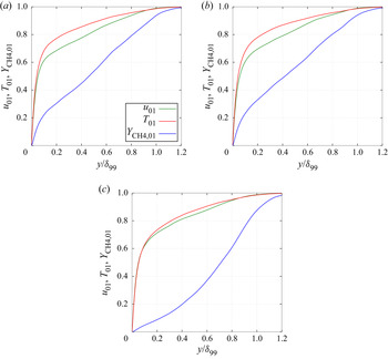
 $Y_{\textrm {CH}4,01}$ are 0 at the wall, and 1 at the far field. Figure 6 shows a comparison of these normalized values. The gradient of the
 $Y_{\textrm {CH}4,01}$ profile is considerably smaller than those of
 $u_{01}$ and
 $T_{01}$ near the wall. Particularly, in the B-T300-600-p60-shifted case, the
 $Y_{\textrm {CH}4,01}$ gradient near the wall is smaller than
 $y/\delta _{99}\simeq 0.8$. This result indicates that the similarity law among velocity, temperature and mass fraction does not hold true.
Comparison at  $Re_{\tau }\approx 500$ of normalized mean profiles of velocity, temperature and mass fraction of methane: (a) B-T300-600-p60, (b) B-T300-600-p80 and (c) B-T300-600-p60-shifted.

5.2.2. Turbulent fluctuations
As already stated, a temporal flow does not achieve a statistically steady state, so that any turbulent fluctuations indicate fluctuations from the Favre average in the homogeneous  $(x,z)$ planes.
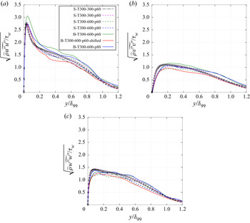
To examine whether the information regarding the mean profiles extends to the fluctuations, these fluctuations are examined in figure 7 which illustrates velocity fluctuations non-dimensionalized by the wall shear stress. The DNS results of the incompressible constant-property turbulent boundary layer by Schlatter & Örlü (Reference Schlatter and Örlü2010) for  $Re_{\tau }=492$ are also included in the figures. Schlatter & Örlü (Reference Schlatter and Örlü2010) make their DNS data publicly available on the URL https://www.mech.kth.se/~pschlatt/DATA/; that database contains the data used here for comparisons. (When
 $Re_{\tau }=492$,
 $Re_{\theta }\simeq 1410$ in their simulation.) The results show that the fluctuation profiles of the present DNS are similar to those of the incompressible DNS data, indicating that the qualitative characteristic of momentum diffusion is the same as that of the incompressible flow, a fact which is attributed to the relatively small value of the Mach number in the compressible regime.
Velocity fluctuations at  $Re_{\tau }\approx 500$ in (a) streamwise, (b) wall-normal and (c) spanwise directions. The legend is the same as in figure 5. Circles represent the DNS results from the incompressible constant-property boundary layer study of Schlatter & Örlü (Reference Schlatter and Örlü2010).

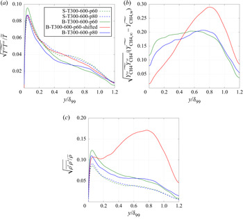
Figure 8 depicts fluctuations of  $T$,
 $Y_{\textrm {CH}4}$ and
 $\rho$. The data of S-T300-300-p60 and S-T300-300-p80 are not included because the fluctuations are almost null in these cases. The temperature fluctuations peak at
 $y/\delta _{99}=0.05$ in all cases. In contrast, the mass fraction fluctuations peak at
 $y/\delta _{99}\simeq 0.6$ in the B-T300-600-p60 and B-T300-600-p80 cases, and peak at
 $y/\delta _{99}\simeq 0.8$ in B-T300-600-p60-shifted. Comparing the binary-species cases, the case B-T300-600-p60-shifted has smaller fluctuations than the other cases near the wall, with larger fluctuations around the centre of the boundary layer. This is because the mass fraction gradient of the B-T300-600-p60-shifted is small near the wall, and becomes large at
 $y/\delta _{99}\simeq 0.8$ as shown in figure 6. These
 $T$ and
 $Y_{\textrm {CH}4}$ fluctuations affect the
 $\rho$ fluctuations. The
 $\rho$ fluctuations peak at
 $y/\delta _{w}=0.05$ in four cases, but the B-T300-600-p60-shifted behaviour is different. Because the
 $T$ fluctuation peaks at the same location as those of
 $\rho$ in the aforementioned four cases, it is conjectured that the peaks in the four cases are due to the strong
 $T$ fluctuations. In contrast, the B-T300-600-p60-shifted peak at
 $y/\delta _{w}=0.8$ is believed to be particularly affected by the larger fluctuations of
 $Y_{\textrm {CH}4}$ close to the centre of the boundary layer.
Fluctuations at  $Re_{\tau }\approx 500$ of (a) temperature, (b) mass fraction of methane and (c) density. Mass fraction profiles are only shown for the binary-species cases.

The comparison of fluctuations between  $T$ and
 $u$ shows that both profiles peak at the same location. In addition, the
 $T$ fluctuations are similar to the
 $u$ fluctuations. This result indicates that the similarity between
 $u$ and
 $T$ fluctuations holds. In contrast,
 $Y_{\textrm {CH}4}$ has the maximum close to the centre of the boundary layer, and there is no sharp peak near the wall. This result corroborates that mass diffusion is not similar to momentum diffusion or thermal diffusion.
5.2.3. Turbulent kinetic energy budget
To investigate whether the TKE may explain the differences between single-species and binary-species cases, the budget of this quantity is examined. The TKE is defined as
 \begin{equation} \tilde{k}=\frac{1}{2}\frac{\overline{\rho u_{i}^{\prime\prime} u_{i}^{\prime\prime}}}{\bar{\rho}}. \end{equation}
The TKE budget equation is
 \begin{equation} \frac{\partial\bar{\rho}\tilde{k}}{\partial t}+\frac{\partial }{\partial x_{j}}( \bar{\rho}\widetilde{u_{j}}\tilde{k}) =P+T+\varPi+\phi_{dif}+\phi_{dis}+M, \end{equation}
where
 \begin{equation} \left. \begin{array}{c} P ={-}\overline{\rho u_{i}^{\prime\prime}u_{i}^{\prime\prime}}\dfrac {\partial\widetilde{u_{i}}}{\partial x_{j}},\\ \displaystyle T ={-}\dfrac{1}{2}\dfrac{\partial}{\partial x_{j}}\left( \overline{\rho u_{i}^{\prime\prime}u_{i}^{\prime\prime}u_{j}^{\prime\prime}},\right) \\ \displaystyle \varPi =\varPi_{t}+\varPi_{d}={-}\dfrac{\partial}{\partial x_{j}}\left( \overline{p^{\prime}u_{j}^{\prime}}\right) +\overline{p^{\prime}\dfrac{\partial u_{i}^{\prime}}{\partial x_{i}}},\\ \displaystyle \phi_{dif} =\dfrac{\partial}{\partial x_{j}}\left( \sigma_{ij}^{\prime }u_{i}^{\prime}\right) ,\\ \displaystyle \phi_{dis} ={-}\overline{\sigma_{ij}^{\prime}\dfrac{\partial u_{i}^{\prime} }{\partial x_{j}}},\\ \displaystyle M =\overline{u_{i}^{\prime\prime}}\left( \dfrac{\partial\overline{\tau_{ij}}}{\partial x_{j}}- \dfrac{\partial\bar{p}}{\partial x_{i} }\right) . \end{array}\right\} \end{equation}
The terms on the right-hand side in (5.3) are as follows:  $P$ denotes the production;
 $T$ labels the turbulent transport;
 $\varPi$ designates the pressure term, which includes pressure diffusion,
 $\varPi _{t},$ and pressure dilatation,
 $\varPi _{d}$;
 $\phi _{dif}$ identifies the viscous diffusion;
 $\phi _{dis}$ denotes the viscous dissipation; and
 $M$ labels the mass flux contribution. Both
 $M$ and
 $\varPi _{d}$ result from non-constant density.
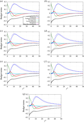
Figure 9 shows the terms in the budget of TKE near the wall. The DNS data by Schlatter & Örlü (Reference Schlatter and Örlü2010) is also included in the figure. The budget terms are non-dimensionalized by  $\tau _{w}^{2}/\bar {\mu }$ (Foysi, Sarkar & Friedrich Reference Foysi, Sarkar and Friedrich2004). The wall-normal coordinates are normalized by
 $y^{\ast }\equiv \bar {\rho }u_{\tau }^{\ast }y/\bar {\mu }$, where
 $u_{\tau }^{\ast }$ is semi-local friction velocity defined by
 $u_{\tau }^{\ast }\equiv \sqrt {\tau _{w} /\bar {\rho }}$ (Huang, Coleman & Bradshaw Reference Huang, Coleman and Bradshaw1995). The budget terms in S-T300-300-p60 and S-T300-300p80 collapse to the incompressible constant-property boundary layer. This result indicates that turbulent statistics of the present temporal boundary layers are faithfully comparable to those of spatial developing boundary layers. In the other cases, due to non-constant density, a negative mass flux contribution appears that peaks at
 $y^{\ast }\approx 10$. However, the negative peak of the mass flux contribution is smaller than the other budget terms, and all budget terms agree well with those of the incompressible boundary layer. Therefore, there is no significant difference in TKE budget between single-species and binary-species boundary layers.
Turbulent kinetic energy budget for cases (a) S-T300-300-p60, (b) S-T300-300-p80, (c) S-T300-600-p60, (d) S-T300-600-p80, (e) B-T300-600-p60, ( f) B-T300-600-p80 and (g) B-T300-600-p60-shifted, all at  $Re_{\tau } \approx 500$. Quantities have been non-dimensionalized by
 $\tau ^{2} _{w}/\bar {\mu }$. Symbols represent the DNS results from the incompressible constant-property boundary layer study of Schlatter & Örlü (Reference Schlatter and Örlü2010).

The flow statistics provided information based on averaging of various quantities. To trace the findings to specific phenomena, the flow structure is examined next. Since the lack of similarity only occurs for  $Y_{\textrm {CH}4}$, the following analysis exclusively focuses on the binary-species cases.
5.3. Flow structure
For the purpose of understanding variations in flow structure, fluctuation data of  $u$,
 $T$ and
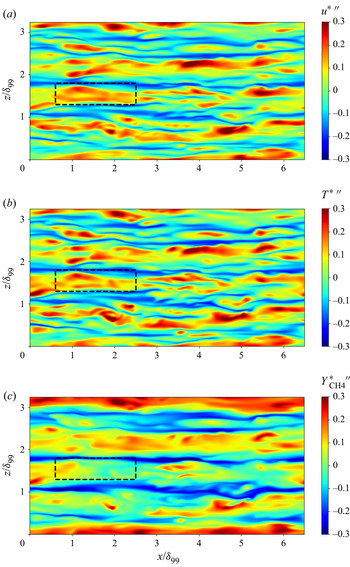
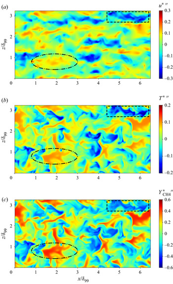
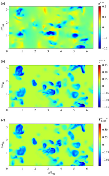
 $Y_{\textrm {CH}4}$ are extracted at various distances from the wall. To investigate the flow structure of the binary-species boundary layer, instantaneous snapshot contours of B-T300-600-p60 are shown in wall-parallel planes in figures 10–12 at different
 $y^{+}$ locations. Figure 10 shows fluctuations at
 $y^{+}=10$, which is representative of the near-wall region; figure 11 illustrates data at
 $y^{+} =250$, which is located at the centre of the boundary layer; and figure 12 depicts information at
 $y^{+}=450$, which is near the edge of the boundary layer. Fluctuations shown in these figures are normalized as
 \begin{equation} {\varTheta^{{\ast}}}^{\prime\prime}=\frac{\varTheta^{\prime\prime}}{\widetilde{\varTheta_{\infty}}-\widetilde{\varTheta_{w}}}, \end{equation}
where  $\varTheta$ is
 $u$,
 $T$ or
 $Y_{\textrm {CH}4}$. Because the wall moves and the far field is at rest, this normalization switches the sign of velocity fluctuations from the original value (the signs of temperature and mass fraction of methane are not switched). The colour legend selected for this normalization is such that a region where
 $\varTheta$ is closer to a wall value is coloured blue, and a region where
 $\varTheta$ is closer to a far field value is coloured red.
Instantaneous snapshot at  $Re_{\tau }\approx 500$ in the
 $y^{+}=10$ (
 $y/\delta _{99}=0.02$) wall-parallel plane for B-T300-600-p60. (a) Streamwise velocity, (b) temperature and (c) mass fraction of methane.

Instantaneous snapshot at  $Re_{\tau }\approx 500$ in the
 $y^{+}=250$ (
 $y/\delta _{99}=0.5$) wall-parallel plane for B-T300-600-p60. (a) Streamwise velocity, (b) temperature and (c) mass fraction of methane.

Instantaneous snapshot at  $Re_{\tau }\approx 500$ in the
 $y^{+}=450$ (
 $y/\delta _{99}=0.92$) wall-parallel plane for B-T300-600-p60. (a) Streamwise velocity, (b) temperature and (c) mass fraction of methane.

The velocity field at  $y^{+}=10$ exhibits the typical streaky structures. The blue-coloured streaks are accompanied by the upward (
 $v^{\prime \prime }>0$) vertical transport of the near-wall fluid, and can be interpreted as ejection events. The red-coloured streaks are accompanied by the downward (
 $v^{\prime \prime }<0$) vertical transport of the upper fluid, and can be interpreted as sweep events. Similar streaky structures were observed in many DNS of compressible boundary layers (Duan et al. Reference Duan, Beekman and Martín2010, Reference Duan, Beekman and Martín2011; Pirozzoli & Bernardini Reference Pirozzoli and Bernardini2011; Kawai Reference Kawai2019). The temperature field at
 $y^{+}=10$ also shows similar streaky structures. The comparison with the velocity field clearly shows that both blue-coloured and red-coloured temperature streaks appear at the same location as the velocity field, and the temperature contour pattern is quite similar to that of the velocity. The coincidence of the contour patterns indicates the well-known similarity between velocity and temperature fluctuations. The contour of mass fraction of methane at
 $y^{+}=10$ also shows streaky structures. However, careful observation reveals that there are some differences between the mass fraction and the other fields. For example, in the region included in the black dashed-line square box, a red-coloured streaky structure was observed in the velocity and temperature fields. In contrast, there is no streaky structure of the mass fraction field in the same region. This contrary behaviour indicates that locally in
 $(x,z)$ planes, mass diffusion is not similar to momentum diffusion and thermal diffusion at
 $y$ locations near the wall.
The velocity field at  $y^{+}=250$ shows that the spanwise spacing and the length of the velocity streaks are wider and shorter than those at
 $y^{+}=10,$ but the streaky structures remain at the centre of the boundary layer. The similarity between the velocity and temperature fields becomes less clear. A blue-coloured streak inside the black dashed-line square box is common between the velocity and temperature contours. In contrast, an orange-coloured streak inside the region surrounded by the dash–dotted line is observed in the velocity field, while a non-streaky structure is observed in the temperature field in the same region. This difference indicates that the similarity between the momentum and thermal diffusion becomes weaker at the centre of the boundary layer. In contrast, the mass fraction contour is quite similar to that of the temperature, and there is no clear difference in shape between them. The coincidence of the contour pattern indicates that the flow physics of mass diffusion is fundamentally the same as that of thermal diffusion at the centre of the boundary layer.
At  $y^{+}=450,$ the streaky velocity structure no longer exists, and intermittent ejections can be observed. Intermittent ejections also appear in the temperature field, but their shape is different. Some temperature ejections are shaped akin to a mushroom-like structure, similar to that reported in supersonic boundary layers by Pirozzoli & Bernardini (Reference Pirozzoli and Bernardini2011). The mass fraction contour is quite similar to that of the temperature and, thus, the similarity between mass and thermal diffusions holds true near the edge of the boundary layer, analogous to the situation at the centre in the wall-normal coordinate.
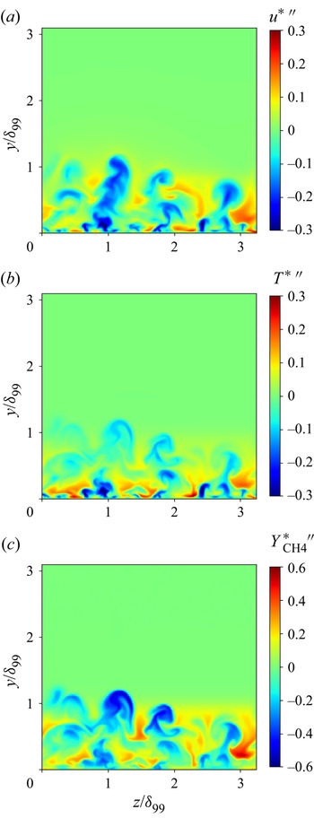
To investigate flow structure variation in the wall-normal direction, snapshot contours are illustrated in figure 13 in the  $x/\delta _{99}=3.25$ plane. The velocity contours show that some blue-coloured ejections near the wall extend to the edge of the boundary layer. Such extension of the ejections cannot be observed in the temperature field. This difference implies that the weakened similarity between the temperature and velocity field at
 $y^{+}=250$ is due to the gap of the ejection events. Although the mass fraction contour in the wall-parallel plane is quite similar to that of the temperature at
 $y^{+}=250$ and
 $450$, the contours in the cross-stream plane are very different. The temperature fluctuations are strong near the wall, and become weaker away from the wall, whereas relatively strong fluctuations of the mass fraction appear near the edge of the boundary layer and the intensity of the fluctuations does not largely vary in the wall-normal direction. These observations are consistent with the fluctuation profiles of figure 8. This result implies either of two scenarios: fluctuations of the mass fraction are suppressed near the wall, or the fluctuations are enhanced away from the wall. However, the second scenario is unlikely, because the contours in wall-parallel planes indicate similarity between the mass and thermal diffusions away from the wall. Therefore, the contours in the cross-stream plane imply the first scenario. To further investigate this scenario, the details of species-mass diffusion are scrutinized.
Instantaneous snapshot at  $Re_{\tau }\approx 500$ in the
 $x/\delta _{99}=3.25$ plane for B-T300-600-p60. (a) Streamwise velocity, (b) temperature and (c) mass fraction of methane.

5.4. Species-mass diffusion
Since turbulent statistics and observation of the flow field reveal that the flow physics of mass diffusion near the wall is different from momentum diffusion and thermal diffusion, the special characteristics of species-mass diffusion involving the Soret effect are investigated. The interest is primarily in the flux in the wall-normal direction. First, the information provided by the mean flow field is investigated, followed by the examination of the instantaneous flow field and finally the turbulent transport is addressed. Included in the study of turbulent transport are the representative non-dimensional numbers quantifying it: the turbulent Schmidt number and turbulent Prandtl number. The study of turbulent transport culminates with a quadrant analysis.
5.4.1. Species-mass diffusion balance in the mean flow field
For the purpose of this analysis, (2.4) is averaged in the homogeneous  $(x,z)$ plane and since through averaging the derivatives in the homogeneous directions are null, the following equation holds:
 \begin{equation} \frac{\partial}{\partial t}\left( \bar{\rho}\widetilde{Y_{\alpha} }\right) +\frac{\partial}{\partial y}\left[ \bar{\rho} \widetilde{Y_{\alpha}}\tilde{v}+\bar{\rho}\widetilde{Y_{\alpha}^{\prime\prime }v^{\prime\prime}}+\overline{J_{\alpha,y}}\right] = 0. \end{equation}
When  $\tilde {v}$ is sufficiently small to be negligible, (5.6) is rewritten as
 \begin{align}
&\frac{\partial}{\partial t}(
\bar{\rho}\widetilde{Y_{\alpha} })
+\frac{\partial}{\partial y}\left[
\bar{\rho}\widetilde{Y_{\alpha}^{\prime\prime}v^{\prime\prime}}-\overline{\rho
Y_{\alpha}( D_{T,\alpha}) \frac{\partial
T}{\partial y}}-\overline{\rho Y_{\alpha }(
D_{p,\alpha}) \frac{\partial p}{\partial
y}}\right.\notag\\
&\quad -\left.\sum_{\beta =1}^{N-1}\overline{\rho\left(
D_{\alpha\beta}^{\prime}\frac{m_{\alpha}
}{m_{\beta}}\right) \frac{\partial Y_{\beta}}{\partial
y}}\right] \simeq0.
\end{align}
Equation (5.7) shows that the  $\alpha$-species species-mass flux for the mean flow field is given by
 \begin{equation} J_{mean}(y)\simeq\bar{\rho}\widetilde{Y_{\alpha}^{\prime\prime} v^{\prime\prime}}-\overline{\rho Y_{\alpha}\left( D_{T,\alpha}\right) \frac{\partial T}{\partial y}}-\overline{\rho Y_{\alpha}\left( D_{p,\alpha }\right) \frac{\partial p}{\partial y}}-\sum_{\beta=1}^{N-1}\overline{\rho\left( D_{\alpha\beta}^{\prime}\frac{m_{\alpha}}{m_{\beta}}\right) \frac{\partial Y_{\beta}}{\partial y}}, \end{equation}
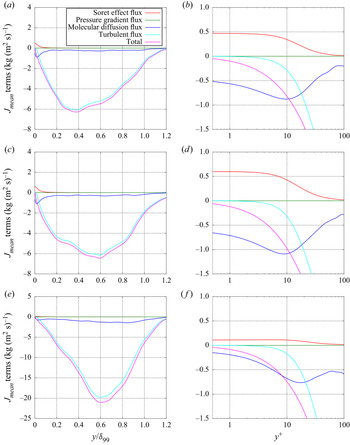
where the first term is the turbulent flux, the second term is the Soret effect flux, the third term is the pressure gradient flux and the forth term is the molecular diffusion flux.
Figure 14 depicts the profiles of these four terms for methane as a function of either  $y/\delta _{99}$ or
 $y^{+}$. Since the mass fraction of methane monotonically increases from the wall, the total mass flux
 $J_{mean}$ is negative in all cases. The turbulent flux and the molecular diffusion flux are also negative because the sign of these fluxes depends on a gradient of mass fraction. In contrast, the Soret effect flux is positive because the coefficient
 $D_{T,\alpha }$ is negative and the derivative
 $\partial T/\partial y$ is positive. The pressure gradient flux is sufficiently small to be negligible in the entire region. The total mass flux is null at the wall, and has a negative peak at
 $y/\delta _{99}=0.4$ in case B-T300-600-p60, and at
 $y/\delta _{99}=0.6$ in cases B-T300-600-p80 and B-T300-600-p60-shifted. The turbulent flux is overwhelmingly larger than the other terms for
 $y^{+}\geqslant 20$. In contrast, the turbulent flux is suppressed for
 $y^{+}\leqslant 20$, and the molecular diffusion flux is the largest, as expected in the near-wall region. In addition, the Soret effect flux becomes relatively large near the wall because of the large temperature gradient.
Species-mass flux of the mean flow field as a function of the outer scaling  $y/\delta _{99}$ (a,c,e) and as a function of the wall unit
 $y^{+}$ (b,d, f): for cases (a,b) B-T300-600-p60, (c,d) B-T300-600-p80 and (e, f) B-T300-600-p60-shifted, all at
 $Re_{\tau }\approx 500$.

It is well known that molecular diffusion is dominant in the viscous sublayer, and velocity and temperature gradients become steeper due to the large molecular diffusion. However, the sign of the Soret effect flux is opposite to that of the molecular diffusion flux, and absolute values of these fluxes are quantitatively similar in the viscous sublayer for  $y^{+} \leqslant 5$, leading to the total mass flux being approximately 0 in the viscous sublayer. The approximately null total mass flux indicates that methane is hardly diffused, and this is the reason why the species-mass fraction remains small near the wall.
5.4.2. Relationship between the molecular diffusion flux and the Soret effect flux
In order to further investigate species-mass diffusion near the wall, the relationship in the instantaneous flow field between molecular diffusion and the Soret effect is here assessed and discussed. The Soret effect operates independent of the prevailing  $p$, however, the value of
 $\bar {\alpha }_{T,\beta }^{b}$ is typically smaller at atmospheric
 $p$ than at high
 $p$, meaning that at the same temperature difference between wall and gas, the Soret effect is much smaller at atmospheric
 $p$ than at high-
 $p$ conditions.
Since the species-mass diffusion balance for the mean flow shows that the pressure gradient flux is sufficiently small to be negligible, the  $\alpha$-species mass flux in the wall-normal direction can be approximated as the sum of the molecular diffusion flux
 $J_{mol,y}$ and the Soret effect flux
 $J_{sor,y}$, i.e.
 \begin{equation} J_{\alpha,y}\approx J_{mol,y}+J_{sor,y}, \end{equation}
where
 $$\begin{gather} J_{mol,y}={-}\sum_{\beta=1}^{N-1}\rho\left( D_{\alpha\beta}^{\prime} \frac{m_{\alpha}}{m_{\beta}}\right) \frac{\partial Y_{\beta}}{\partial y}, \end{gather}$$
 $$\begin{gather}J_{sor,y}={-}\rho Y_{\alpha}\left( D_{T,\alpha}\right) \frac{\partial T}{\partial y}. \end{gather}$$
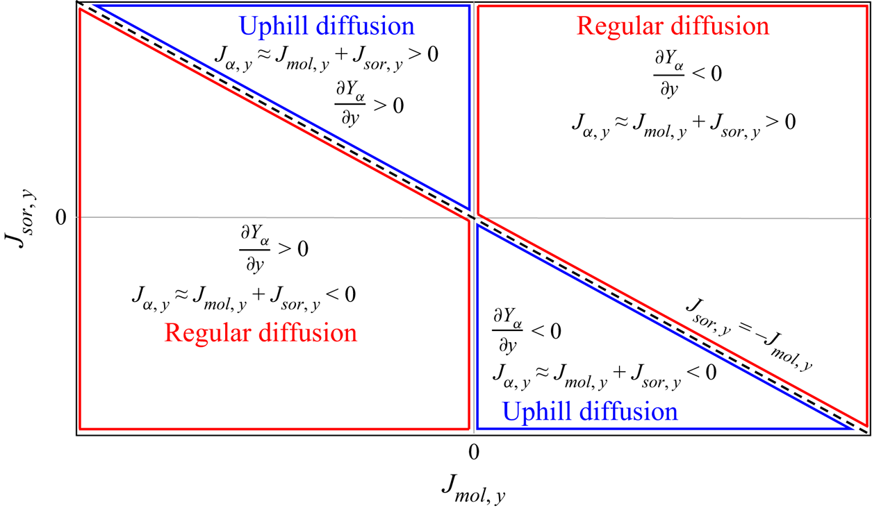
In the past, species-mass diffusion has been classified as either regular or uphill (Taylor & Krishna Reference Taylor and Krishna1993; Sciacovelli & Bellan Reference Sciacovelli and Bellan2019). This classification was introduced for isothermal and isobaric situations related to the original experiment of Duncan & Toor (Reference Duncan and Toor1962) discovering uphill diffusion. Under those conditions, uphill diffusion occurs due to strong coupling among fluxes when there are more than two species, and it is manifested by the signs of  $J_{\alpha ,y}$ and
 $\partial Y_{\alpha }/\partial y$ being the same, that is, by the flux of the species being directed from regions of small concentrations of that species to regions of large concentrations. In contrast, regular diffusion occurs when the signs of
 $J_{\alpha ,y}$ and
 $\partial Y_{\alpha }/\partial y$ are different, so that the flux is directed from regions of large concentrations to regions of low concentration. However, the present situation is neither isothermal nor isobaric. Moreover, in a binary-species flow, the molecular diffusion flux never occurs against the mass fraction gradient, although the Soret effect flux can be against the mass fraction gradient because the Soret effect flux depends on the temperature gradient, not the mass fraction gradient. Therefore, if the original definition of uphill diffusion is retained, the Soret effect flux may cause uphill diffusion in a binary-species flow, unlike in isothermal and isobaric flows in which this phenomenon was originally observed. Figure 15 illustrates this new concept. When the signs of
 $J_{mol,y}$ and
 $J_{sor,y}$ are the same, regular diffusion occurs. When the signs of
 $J_{mol,y}$ and
 $J_{sor,y}$ are different, the interface between the regular and uphill diffusion is determined by the line of
 $J_{sor,y} =-J_{mol,y}$. If
 $J_{sor,y}$ is against and larger in absolute value than
 $J_{mol,y}$, uphill diffusion occurs because the sum of these fluxes is against the mass fraction gradient. If the
 $J_{sor,y}$ is against but smaller in absolute value than
 $J_{mol,y}$, regular diffusion occurs. The previous mechanism for uphill diffusion (Taylor & Krishna Reference Taylor and Krishna1993; Sciacovelli & Bellan Reference Sciacovelli and Bellan2019) is completely different from the uphill diffusion due to the Soret effect. Thus, here a new mechanism has been identified – Soret-induced uphill diffusion – which is crucial to explaining species-mass diffusion in boundary layers when there is a temperature gradient between the wall and the fluid flow.
Diagram illustrating the classification of mass diffusion events.

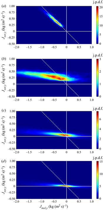
To analyse the interactions between  $J_{sor,y}$ and
 $J_{mol,y}$ at different boundary layer heights, the joint probability density function (j.p.d.f.) of
 $J_{mol,y}$ and
 $J_{sor,y}$ for B-T300-600-p60 at
 $y^{+}=0.3$,
 $10$,
 $30$ and
 $50$ is illustrated in figure 16. The line
 $J_{sor,y}=-J_{mol,y}$ is shown in each figure to locate the j.p.d.f. with respect to this crucial boundary between regular and uphill diffusion. The j.p.d.f.s are computed using
 $(x,z)$ plane data at each location. At
 $y^{+}=0.3,$ the j.p.d.f. shows that the probability density is concentrated near the
 $J_{sor,y}=-J_{mol,y}$ line. The concentration near the line indicates that
 $J_{mol,y}$ and
 $J_{sor,y}$ are balanced and the total species-mass flux is approximately 0 in almost the entire area. This result is consistent with the species-mass diffusion balance shown in figure 14. A peak of the j.p.d.f. at
 $y^{+}=10$ is located at
 $(J_{mol,y},J_{sor,y})=(-0.3,0.2)$. The different sign of
 $J_{mol,y}$ and
 $J_{sor,y}$ indicates that the Soret effect flux is primarily preventing the species-mass diffusion. At
 $y^{+}=10,$
 $J_{mol,y}$ extends over a wide region of values from
 $-2.0$ to
 $0.5$, while
 $J_{sor,y}$ concentrates in a narrow band between 0.2 and 0.5. Significantly, the j.p.d.f. overlaps with the upper uphill diffusion region. This result clearly shows that Soret-induced uphill diffusion occurs at
 $y^{+}=10$. Soret-induced uphill diffusion inevitably makes Fick's law invalid for the species-mass diffusion for binary-species systems, and the similarity law between the thermal and species-mass diffusions also becomes invalid. Therefore, the j.p.d.f. indicates that the difference between the temperature and mass fraction fields at
 $y^{+}=10$ (figure 10) results from Soret-induced uphill diffusion. At
 $y^{+}=30$ and
 $50$, the j.p.d.f.s show that the regions of significant values are located near the null axis of the
 $J_{sor,y}$ because the temperature gradient decreases further away from the wall. As
 $J_{sor,y}$ becomes smaller, Soret-induced uphill diffusion occurs less frequently. In addition, when
 $J_{sor,y}$ is sufficiently small to be negligible, the mass flux
 $J_{\alpha ,y}$ in a binary-species flow can be approximated as Fick's law and the similarity law between the mass and thermal diffusions is recovered. This consideration is supported by the similarity between the temperature and mass fraction field at
 $y^{+}=250$ and
 $450$ (figures 11 and 12).
Joint probability density function of  $J_{mol,y}$ and
 $J_{sor,y}$ at
 $Re_{\tau }\approx 500$ for B-T300-600-p60: (a) at
 $y^{+}=0.3$, (b)
 $y^{+}=10$, (c)
 $y^{+}=30$ and (d)
 $y^{+}=50$. The solid white lines are null axes, and the white broken line is given by
 $J_{sor,y}=-J_{mol,y}$.

Of note, because for the  $\textrm {CH}_{4}/\textrm {N}_{2}$ mixture the value of
 $\bar {\alpha }_{T,\beta }^{b}$ is not a strong function of pressure, with increasing
 $p$ the absolute value of the corresponding term in the species flux is a stronger function of
 $\boldsymbol {\nabla } T$ than of the multiplying coefficient. Under atmospheric-
 $p$ situations species-mass diffusion is much larger (typically by
 $O(10^{2})$; see Masi et al. Reference Masi, Bellan, Harstad and Okong'o2013) than at higher
 $p$ and, thus,
 $\boldsymbol {\nabla }\rho$ is much smaller; since
 $\boldsymbol {\nabla } T$ is related to
 $\boldsymbol {\nabla }\rho$ through the EOS, this means that
 $\boldsymbol {\nabla } T$ will be considerably larger at large
 $p$ than at atmospheric
 $p$. Therefore, for otherwise same initial conditions at high
 $p$, it is much more likely to expect Soret effect induced uphill diffusion than at atmospheric
 $p$. For example, no uphill diffusion was observed in previously performed simulations for high-
 $p$ binary-species mixing layers (Okong'o & Bellan Reference Okong'o and Bellan2002; Okong'o et al. Reference Okong'o, Harstad and Bellan2002) in absence of a wall, indicating that the crucial condition leading here to a very large Soret effect is the large
 $\boldsymbol {\nabla } T$ at the wall. Furthermore, with increasing
 $p$, nonlinearities increase and the species-mass fluxes become increasingly coupled, compounding the possibility of obtaining uphill diffusion.
5.4.3. Comparison of species-mass and thermal turbulent transport
The impact of Soret-induced uphill diffusion on the turbulent non-dimensional numbers is here examined, and the influence of Soret-induced uphill diffusion in determining the mass fraction of the species in different regions of the flow is assessed.
5.4.3.1 Turbulent Prandtl and Schmidt numbers
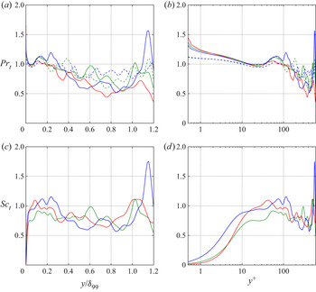
Figure 17 illustrates the turbulent Prandtl number and turbulent Schmidt number defined as
 $$\begin{gather} Pr_{t} =\frac{\left[ -\bar{\rho}\widetilde{u^{\prime\prime} v^{\prime\prime}}\right] \partial\tilde{T}/\partial y}{\left[ -\bar{\rho}\widetilde{v^{\prime\prime}T^{\prime\prime}}\right] \partial\tilde{u}/\partial y}, \end{gather}$$
 $$\begin{gather}Sc_{t} =\frac{\left[ -\bar{\rho}\widetilde{u^{\prime\prime} v^{\prime\prime}}\right] \partial\widetilde{Y_{\textrm{CH}4}}/\partial y}{\left[ -\bar{\rho}\widetilde{v^{\prime\prime}Y_{\textrm{CH}4}^{\prime\prime}}\right] \partial\tilde{u}/\partial y}. \end{gather}$$
Each  $Pr_{t}$ and
 $Sc_{t}$ are depicted as functions of both
 $y/\delta _{99}$ and
 $y^{+}.$ The
 $Pr_{t}$ value is approximately 1 for
 $y/\delta _{99}<0.2$, a fact which reflects strong similarity of turbulent transport for temperature and momentum. The
 $Pr_{t}$ value slightly decreases for
 $y/\delta _{99}>0.2$ (
 $y^{+}>100$), a fact which is a manifestation of the weaker similarity between the temperature and velocity field at the centre of the boundary layer. The qualitative aspects of
 $Pr_{t}$ are common between the single-species and binary-species cases, indicating that turbulent thermal diffusion in binary-species flows is qualitatively the same as in single-species flow. Here
 $Sc_{t}$ shows similar behaviour to
 $Pr_{t}$ for
 $y/\delta _{99}>0.2$, but its near-wall trend is different from that of
 $Pr_{t}$. Particularly, for
 $y^{+}<10$,
 $Sc_{t}$ has values considerably less than 1 for all binary-species cases, indicating reduced similarity of turbulent transport of mass and momentum near the wall.
Turbulent Prandtl number and turbulent Schmidt number at  $Re_{\tau }\approx 500$ as a function of the outer scaling
 $y/\delta _{99}$ (a,c) and as a function of the wall unit
 $y^{+}$ (b,d): (a,b) turbulent Prandtl number and (c,d) turbulent Schmidt number. The legend is the same as in figure 5.

5.4.3.2 Quadrant contributions to turbulent fluxes
A powerful method to investigate the similarities and differences among phenomena is quadrant analysis. Details about quadrant analysis may be found in Wallace (Reference Wallace2016). The goal here is to investigate quadrant contributions to the Reynolds stress  $\bar {\rho }\widetilde {u^{\prime \prime } v^{\prime \prime }}$, the turbulent heat flux
 $\bar {\rho }\widetilde {v^{\prime \prime }T^{\prime \prime }}$ and the turbulent mass flux of methane
 $\bar {\rho }\widetilde {v^{\prime \prime }Y_{\textrm {CH}4}^{\prime \prime }}$ where quadrants are classified for these turbulent fluxes in four categories:
 $\textrm {Q}1(\theta ^{\prime \prime }>0,v^{\prime \prime }>0)$,
 $\textrm {Q}2(\theta ^{\prime \prime }<0,v^{\prime \prime }>0)$,
 $\textrm {Q}3(\theta ^{\prime \prime }<0,v^{\prime \prime }<0)$ and
 $\textrm {Q}4(\theta ^{\prime \prime }>0,v^{\prime \prime }<0)$, with
 $\theta$ being
 $-u$,
 $T$ or
 $Y_{\textrm {CH}4}$. The sign of
 $u$ is negative because the wall moves and the far field remains at rest in the present simulations. The Q2 and Q4 motions are related to ejection and sweep events, respectively, and they have a positive contribution to the turbulent fluxes. For example, in the present flows, a low-temperature region is ejected by the Q2 motion and a high-temperature region is swept by the Q4 motion. The ejection and sweep mainly generate turbulent fluxes. However, Wallace, Eckelmann & Brodkey (Reference Wallace, Eckelmann and Brodkey1972) clarified that the ejection and sweep contribute turbulent fluxes that are more than 100 % of the average values and indicated that an ejected fluid parcel is pushed back towards the wall and a swept one is reflected away from the wall. The parcel which has either been pushed back or reflected away generates an opposite flux to either the ejection or sweep, and such opposite flux corresponds to either the Q1 or Q3 motion. These regions of parcels pushed back and reflected away were observed in many studies, and the quadrant analysis has been useful to investigate the contribution of each motion (Wallace Reference Wallace2016).
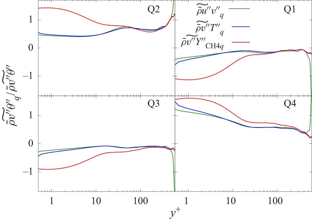
The turbulent fluxes are decomposed and assigned to quadrant contributions and their profiles are shown in figure 18. The contributions of each motion is computed by averaging the turbulent fluxes over  $(x,z)$ planes as
 \begin{equation} \bar{\rho}\widetilde{v^{\prime\prime}\theta^{\prime\prime}} =\overline{\rho v^{\prime\prime}\theta^{\prime\prime}}=\frac{1}{N_{x}N_{z} }\sum_{k=1}^{N_{z}}\sum_{i=1}^{N_{x}}\left( \rho v^{\prime\prime} \theta^{\prime\prime}\right) _{ik}. \end{equation}
The turbulent fluxes can be decomposed to
 \begin{equation} \bar{\rho}\widetilde{v^{\prime\prime}\theta^{\prime\prime}}=\sum _{q=1}^{4}{\bar{\rho}\widetilde{v^{\prime\prime}\theta^{\prime\prime}} }_{q}, \end{equation}
where  $\bar {\rho }\widetilde {v^{\prime \prime }\theta ^{\prime \prime }}_{q}$ is the
 $q$th quadrant contribution given as
 $$\begin{gather} {\bar{\rho}\widetilde{v^{\prime\prime}\theta^{\prime\prime}}}_{1} =\frac{1}{N_{x}N_{z}}\left( \sum_{\substack{k=1\\\theta^{\prime\prime }>0,v^{\prime\prime}>0}}^{N_{z}}\ \sum_{\substack{i=1\\\theta^{\prime\prime }>0,v^{\prime\prime}>0}}^{N_{x}}\left( \rho v^{\prime\prime}\theta ^{\prime\prime}\right) _{ik}\right) , \end{gather}$$
 $$\begin{gather}{\bar{\rho}\widetilde{v^{\prime\prime}\theta^{\prime\prime}}}_{2} =\frac{1}{N_{x}N_{z}}\left( \sum_{\substack{k=1\\\theta^{\prime\prime }<0,v^{\prime\prime}>0}}^{N_{z}}\ \sum_{\substack{i=1\\\theta^{\prime\prime }<0,v^{\prime\prime}>0}}^{N_{x}}\left( \rho v^{\prime\prime}\theta ^{\prime\prime}\right) _{ik}\right) , \end{gather}$$
 $$\begin{gather}{\bar{\rho}\widetilde{v^{\prime\prime}\theta^{\prime\prime}}}_{3} =\frac{1}{N_{x}N_{z}}\left( \sum_{\substack{k=1\\\theta^{\prime\prime }<0,v^{\prime\prime}<0}}^{N_{z}}\ \sum_{\substack{i=1\\\theta^{\prime\prime }<0,v^{\prime\prime}<0}}^{N_{x}}\left( \rho v^{\prime\prime}\theta ^{\prime\prime}\right) _{ik}\right) , \end{gather}$$
 $$\begin{gather}{\bar{\rho}\widetilde{v^{\prime\prime}\theta^{\prime\prime}}}_{4} =\frac{1}{N_{x}N_{z}}\left( \sum_{\substack{k=1\\\theta^{\prime\prime }>0,v^{\prime\prime}<0}}^{N_{z}}\ \sum_{\substack{i=1\\\theta^{\prime\prime }>0,v^{\prime\prime}<0}}^{N_{x}}\left( \rho v^{\prime\prime}\theta ^{\prime\prime}\right) _{ik}\right) . \end{gather}$$
Quadrant contributions to Reynolds stress, turbulent heat flux and turbulent mass flux of methane in B-T300-600-p60 at  $Re_{\tau }\approx 500$.

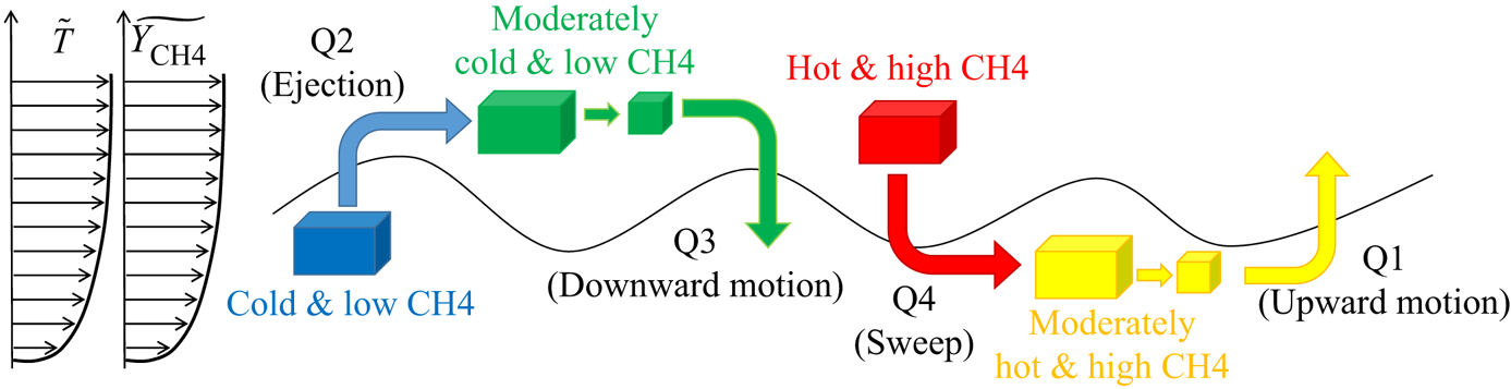
Figure 18 shows that contributions of the Q2 and Q4 motions are positive and those of the Q1 and Q3 motions are negative for all flux profiles. The negative contributions of the Q1 and Q3 motions indicate that regions where the fluid has been either pushed back or reflected away occur in the present situation. These quadrant contributions for the examined simulation are conceptually sketched in figure 19. In the present binary-species simulations, the mean temperature increases in the direction away from the wall. Therefore, figure 19 shows that the lower cold fluid is ejected and that the upper hot fluid is swept. Similarly, the mass fraction of methane also increases in the direction away from the wall and, thus, a small amount of methane is ejected and the enriched fluid with methane is swept. A comparison among the fluxes in figure 18 shows that the heat flux distribution correlates well with the information obtained from the Reynolds stresses but disagrees with the information on the species turbulent flux. The agreement supports the similarity of turbulent transport for temperature and momentum. Inspecting values of the Reynolds stress and turbulent heat flux, positive contributions of the Q2 and Q4 motions are found to be much larger than negative contributions of the Q1 and Q3 motions. This result indicates that a region containing fluid pushed back or reflected away does exist, however, its negative contribution to the Reynolds stress and turbulent heat flux is small, and the result is that the Q2 and Q4 motions are dominant in the Reynolds stress and turbulent heat flux. The distributions of the turbulent species-mass flux collapse to those of the heat flux for  $y^{+}>200$, indicating a similarity of turbulent transport between species mass and temperature. In contrast, the distributions are much different for
 $y^{+}<30$, and especially the negative contributions of the Q1 and Q3 motions are close to
 $-1$. This result indicates that the contributions of the Q1 and Q3 motions become substantial. Therefore, to understand the flow dynamics of turbulent species-mass transport, all quadrant motions including those of Q1 and Q3 should be investigated. Although not shown, the results of the quadrant contributions for the other binary-species cases are qualitatively the same.
Sketch of quadrant contributions.

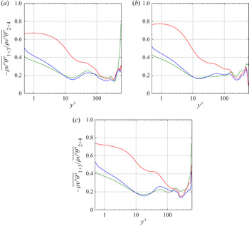
To compare the negative and positive contributions for the three types of fluxes, the sum of the Q1 and Q3 contributions and that of Q2 and Q4 contributions are computed. Figure 20 illustrates these ratios vs  $y^{+}$ in all binary-species cases. For the Reynolds stresses and in the
 $y^{+}<10$ region, the ratio decreases with increasing
 $y^{+}$, and it is approximately 0.2 for
 $y^{+}>10$. The ratio of the turbulent heat flux is qualitatively the same as for the Reynolds stress. These results indicate that for both
 $\bar {\rho }\widetilde {u^{\prime \prime }v^{\prime \prime }}$ and
 $\bar {\rho }\widetilde {v^{\prime \prime }T^{\prime \prime }},$ contributions of the Q1 and Q3 motions are significantly smaller than those of the Q2 and Q4 motions. In contrast, the ratio of the turbulent species-mass flux is relatively larger for
 $y^{+}<100$ than for the other fluxes, and particularly it is larger than 0.5 for
 $y^{+}<10$. This result indicates that, similarly to the other two types of fluxes, the Q2 and Q4 motions are primarily responsible for the generation (see the positive contributions in Q2 and Q4 in figure 18) of the turbulent species-mass flux. However, contrary to the other two types of fluxes, more than 50 % of the generated species-mass flux returns (see negative contributions in figure 18) due to the Q1 and Q3 motions. The physics of the large negative contributions can be explained as follows. Parcels of small methane concentration near the wall are ejected by a Q2 motion. The ejected parcels mix with the surrounding fluid having a larger methane concentration, and the concentration of methane of these parcels would tend to increase due to the molecular diffusion. However, as shown in § 5.4, the Soret effect flux opposes molecular species-mass diffusion due to the high-temperature gradient near the wall, and reduces the total species-mass flux. Therefore, the ejected fluid maintains a small methane concentration. The fluid parcel related to the Q3 motion comes from the formerly ejected parcel and, thus, this fluid parcel maintains a small methane concentration. When the small methane-concentration parcel is pushed back towards the wall, it generates the large negative flux contribution as seen in figure 18. The opposite occurs for the Q4 sweep and Q1 motion. Thus, parcels having small species concentration tend to be trapped near the wall.
Ratio of negative and positive quadrant contributions at  $Re_{\tau }\approx 500$. Here
 $\bar {\rho }\widetilde {v^{\prime \prime }\theta ^{\prime \prime }}_{1+3}$ is the sum of the Q1 and Q3 contributions and
 $\bar {\rho }\widetilde {v^{\prime \prime }\theta ^{\prime \prime }}_{2+4}$ is the sum of the Q2 and Q4 contributions: (a) B-T300-600-p60, (b) B-T300-600-p80 and (c) B-T300-600-p60-shifted. The legend is as in figure 18.

6. Conclusions
Direct numerical simulation of temporal boundary layers at high-pressure conditions has been conducted to investigate the differences and similarities between the single-species and binary-species situations with the focus on species-mass diffusion. The working fluid for the single-species cases is nitrogen and that for the binary-species cases is a mixture of nitrogen and methane. The initial pressure is 60 or 80 atm. After showing that a self-similarity becomes established in these unsteady flows, results from all simulations have been analysed at a similar value of the friction Reynolds number,  $Re_{\tau }\approx 500$ for which the flow is shown to exhibit turbulent characteristics. Examination of these temporal boundary layers elucidated several aspects of their behaviour.
The analysis at  $Re_{\tau }\approx 500$ showed that mean profiles of the streamwise velocity and temperature exhibit steep gradients near the wall, whereas the mass fraction profile does not have a steep gradient near the wall, a fact traced to the different types of boundary conditions. In addition, a comparison of non-dimensionalized values between streamwise velocity, temperature and mass fraction indicated that the similarity law among these profiles does not hold true in the binary-species cases. The fluctuation profiles showed that the qualitative characteristics of velocity fluctuations for high-pressure boundary layers are the same as those of incompressible constant-property boundary layers, a fact attributed to the relatively modest value of the Mach number in the compressible regime. A comparison between velocity and temperature fluctuations indicated that these fluctuations are similar, however, the fluctuations of mass fraction are largely different from those of velocity and temperature. Thus, species-mass diffusion is not similar to momentum and thermal diffusion in binary-species boundary layers under these conditions. The budget of TKE near the wall revealed that the terms due to non-constant density are relatively small, and there is no significant difference in TKE budget between single-species and binary-species boundary layers, thus indicating that the lack of self-similarity cannot be attributed to density spatio-temporal variations.
The flow field in wall-parallel planes is shown to exhibit streaky structures of the streamwise velocity and temperature near the wall, and their fields are similar. However, the mass fraction field at the same location is different from the streamwise velocity and temperature, indicating that mass diffusion is not similar to momentum and thermal diffusion near the wall. Nevertheless, the comparisons at the centre of the boundary layer and near the edge of the boundary layer indicated that the mass fraction field becomes similar to the temperature field, thus implying that the mass diffusion is similar to the thermal diffusion away from the wall. Examination of wall-perpendicular planes indicated that the temperature fluctuations are stronger near the wall and become weaker away from the wall, whereas the mass fraction has relatively strong fluctuations near the edge of the boundary layer, thus implying that the fluctuations of the mass fraction are suppressed near the wall.
Investigation of the species-mass diffusion balance for mean flow fields revealed that the boundary condition combined with high-pressure effects induce the Soret effect flux to become relatively large near the wall. Since the species-mass diffusion flux is null at the wall, the direction of the Soret flux is opposite to the molecular diffusion flux for the initial specification of the wall colder than the fluid. In addition, the analysis of j.p.d.f.s clarified that the Soret effect flux is not only oriented against the species-mass molecular diffusion flux at the wall but that it is occasionally larger in magnitude there than the molecular diffusion flux and, thus, induces uphill diffusion. This mechanism of uphill diffusion is completely different from that previously reported and defined for isothermal and isobaric systems; that type of uphill diffusion cannot occur for a binary-species system. Thus, we have discovered a previously unreported physical mechanism – Soret-induced uphill diffusion – which is promoted at high pressure for binary species, and also presumably multi-species, when heat transfer is large. Under these circumstances, Fick's molecular diffusion flux cannot represent the total species-mass flux. Examination of the j.p.d.f.s also revealed that the Soret flux becomes smaller away from the wall, as expected, explaining why the similarity between the mass and thermal diffusions becomes operative at those locations.
Assessment of turbulent Prandtl number profiles indicated that turbulent thermal transport for the binary-species case is qualitatively the same as that of the single-species case. In contrast, the turbulent Schmidt number becomes small near the wall, and its behaviour is different from that of the turbulent Prandtl number. An analysis based on quadrant contributions elucidated the role of the Soret effect in essentially trapping small species-concentration parcels of fluid in the wall vicinity due to the negative contribution of the Soret effect flux.
Acknowledgements
The authors thank Dr M. Kozul for detailed information about her study of incompressible temporal mixing layers. Computational resources were provided by the JPL Supercomputing Center, by NASA Advanced Supercomputing at Ames Research Center under the T3 program directed by Dr M.M. Rogers.
Funding
This work was conducted at the Jet Propulsion Laboratory (JPL) of the California Institute of Technology (Caltech) and sponsored by the Department of Energy (DOE), Basic Energy Sciences (BES) under the direction of Drs Wade Sisk, with the DOE grant number DE-SC0002679.
Declaration of interests
The authors report no conflict of interest.
Appendix A. Diffusion coefficient calculation
Matrix elements  $\mathbb {D}_{\beta \gamma }$ of (2.8a,b)–(2.9) are the solution of the mixing rules equations (Harstad & Bellan Reference Harstad and Bellan2004)
 \begin{equation} \sum_{\beta=1}^{N}\left[ \delta_{\alpha\beta}-\left( 1-\delta_{\alpha\beta }\right) X_{\beta}\frac{\mathcal{\bar{D}}_{\alpha}}{\mathcal{D}_{\alpha\beta }^{b}}\right] \frac{\mathbb{D}_{\beta\gamma}}{X_{\beta}}=\mathcal{\bar{D} }_{\alpha}\frac{\left( \delta_{\alpha\gamma}-Y_{\alpha}\right) }{X_{\alpha}}, \end{equation}
where
 \begin{equation} \mathcal{\bar{D}}_{\alpha}=1\left/\sum_{\substack{\beta=1\\ \beta\!{\neq}\alpha }}^{N}\left( \dfrac{X_{\beta}}{\mathcal{D}_{\alpha\beta}^{b}}\right) \right.. \end{equation}
Solutions for  $\mathbb {D}_{\beta \gamma }$ may be obtained by an approximate inversion (Ern & Giovangigli Reference Ern and Giovangigli1998) as follows:
 $$\begin{gather} \mathbb{D}_{\beta\gamma} \simeq X_{\beta}\mathbb{D}_{\beta\gamma}^{\left( 1\right) }, \end{gather}$$
 $$\begin{gather}\mathbb{D}_{\alpha\beta}^{\left( 1\right) } = \frac{\left( 1+Y_{\alpha }\right) }{X_{\alpha}}\mathcal{D}_{\alpha}^{{\ast}}\delta_{\alpha\beta}+( 1-\delta_{\alpha\beta}) \frac{\mathcal{D}_{\alpha}^{{\ast}} \mathcal{D}_{\beta}^{{\ast}}}{\mathcal{D}_{\alpha\beta}^{b}}-( \sigma_{\alpha}\mathcal{D}_{\alpha}^{{\ast}}+\sigma_{\beta}\mathcal{D}_{\beta }^{{\ast}}) +\sum_{\gamma=1}^{N}( Y_{\gamma}\sigma_{\gamma }\mathcal{D}_{\gamma}^{{\ast}}) , \end{gather}$$
 $$\begin{gather}\mathcal{D}_{\alpha}^{{\ast}} =\left( 1-Y_{\alpha}\right) \bar{\mathcal{D}}_{\alpha}, \end{gather}$$
 $$\begin{gather}\sigma_{\alpha} =\frac{m_{\alpha}}{m}\left( 1+Y_{\alpha}\right) +\sum_{\substack{\beta=1\\ \beta\!{\neq}\alpha}}^{N}Y_{\beta}\frac{\mathcal{D} _{\beta}^{{\ast}}}{\mathcal{D}_{\alpha\beta}^{b}}. \end{gather}$$
Here  ${\mathcal {D}_{\alpha \beta }^{b}}$ is the full approximation binary-diffusion matrix. This method leads to a singularity when the mixture is composed of only one species (as, for instance, in pure fuel zones). In that case (A2) is no longer used and the diffusion coefficients are evaluated using the binary-diffusion matrix, by setting
 $\mathcal {D}_{\alpha }^{\ast }=$
 $\mathcal {D}_{\alpha N}^{b}$, where
 $N$ represents the index associated with the solvent. This method was tested against an exact Gauss inversion (not shown) and it gave the same results, with an additional gain in computational time. Defining
 $\mathcal {D} _{\alpha \beta }$ as the first approximation of the binary-diffusion matrix and realizing that the deviation of the ratio
 $\mathcal {D}_{\alpha \beta } ^{b}/\mathcal {D}_{\alpha \beta }$ from unity is comparable to uncertainties in binary-diffusion coefficient values (Harstad & Bellan Reference Harstad and Bellan2004), we assume that
 $\mathcal {D}_{\alpha \beta }^{b}=\mathcal {D}_{\alpha \beta }$. The computation of
 ${\mathcal {D}_{\alpha \beta }^{{}}}$ and
 $\alpha _{T,\alpha \beta }^{b}$ is described in references of Masi et al. (Reference Masi, Bellan, Harstad and Okong'o2013) and Sciacovelli & Bellan (Reference Sciacovelli and Bellan2019) along with the other transport properties.
Appendix B. Relationships for the EOS
Miscellaneous relationships relevant to the EOS are
 \begin{equation} a_{mix}=\sum_{\alpha}\sum_{\gamma}X_{\alpha}X_{\gamma}a_{\alpha\gamma}\left( T\right) ,\quad{} b_{mix}=\sum_{\alpha}X_{\alpha}b_{\alpha}, \end{equation}
where indices do not follow the Einstein notation, and
 \begin{align} a_{\alpha\gamma}&=(1-k_{\alpha\gamma}^{\prime})\sqrt{\alpha_{\alpha\alpha }\alpha_{\gamma\gamma}},\end{align}
 \begin{align} \alpha_{\alpha\alpha}(T) & \equiv0.457236(R_{u}T_{c,\alpha})^{2}\nonumber\\ &\quad\times \frac{\left[ 1+c_{\alpha}(1-\sqrt{T_{red,\alpha}})\right] ^{2} }{p_{c,\alpha}}, \end{align}
 \begin{align} c_{\alpha}&=0.37464+1.54226\varOmega_{\alpha}-0.26992\varOmega_{\alpha}^{2}, \end{align}
where  $T_{red,\alpha }\equiv T/T_{c,\alpha },$
 $T_{c,\alpha }$ is the critical temperature and
 $\varOmega _{\alpha }$ is the acentric factor. Also,
 $$\begin{gather} b_{\alpha}=0.077796\dfrac{R_{u}T_{c,\alpha}}{p_{c,\alpha}}, \end{gather}$$
 $$\begin{gather}T_{c,\alpha\gamma}=\left( 1-k_{\alpha\gamma}\right) \sqrt{T_{c,\alpha }T_{c,\gamma}}\quad \text{with }k_{\alpha\alpha}=0, \end{gather}$$
 $$\begin{gather}v_{c,\alpha\gamma}=\tfrac{1}{8}\left( v_{c,\alpha}^{1/3}+v_{c,\gamma} ^{1/3}\right) ^{3}, \end{gather}$$
 $$\begin{gather}Z_{c,\alpha\gamma}=\tfrac{1}{2}\left( Z_{c,\alpha}+Z_{c,\gamma}\right) , \end{gather}$$
 $$\begin{gather}p_{c,\alpha\gamma}=\dfrac{R_{u}T_{c,\alpha\gamma}Z_{c,\alpha\gamma} }{v_{c,\alpha\gamma n}}, \end{gather}$$
with  $T_{red,\alpha \gamma }\equiv T/T_{c,\alpha \gamma },Z_{c,\alpha }$ being the critical compression factor with the compression factor defined as
 $Z=p/(\rho TR_{u}/m)$,
 $v_{c,\alpha }$ being the critical volume,
 $p_{c,\alpha }$ being the critical pressure and
 $k_{\alpha \gamma }$ is an empirical mixing parameter. The relationship between parameters
 $k_{\alpha \gamma }$ and
 $k_{\alpha \gamma }^{\prime }$ is
 \begin{equation} (1-k_{\alpha\gamma})=(1-k_{\alpha\gamma}^{\prime})\frac{(v_{c,\alpha }v_{c,\gamma})^{1/2}}{v_{c,\alpha\gamma}}. \end{equation}
For  $\textrm {N}_{2}/\textrm {CH}_{4}$,
 $k^{\prime }=$0.0311 (Knapp et al. Reference Knapp, Döring, Oellrich, Plöcker and Prausnitz1982).
Appendix C. Stability analysis for perturbations of initial profiles
The perturbations of the initial profiles are derived using stability analysis with the objective to accelerate the attainment of turbulent transition. The stability analysis is performed using inviscid equations because in many experimental situations it has been observed that the most unstable wavelength dominates spatial mixing; for temporal mixing layers, the most unstable wavelength would have the fastest growth rate and reach large Reynolds numbers fastest. Thus, at the  ${Re}$ values of present interest, the development of large structures will be determined by inviscid instabilities. Here, the perturbed flow variables
 $\psi =(\rho ,u,p)$ are given by
 $\psi =\bar {\psi }+\Delta \psi$, where
 $\overline {(\cdot )}$ denotes the mean flow variables, which are functions of
 $y$ only. The perturbations are given by
 \begin{equation} \Delta\psi=\hat{\psi}(y)\exp\left[ \textrm{i}\alpha(x\cos\phi+z\sin\phi -ct)\right] , \end{equation}
where  $\widehat {(\cdot )}$ denotes the perturbation amplitudes and, for temporal analysis,
 $\alpha$ is real and
 $c$ is complex. The functional form of the perturbation in the
 $(x,z)$ plane is chosen so that the unit vector makes an angle
 $\phi$ with the streamwise direction. The streamwise and spanwise wavelengths are
 $\lambda _{1}=2{\rm \pi} /(\alpha \cos \phi )$ and
 $\lambda _{3} =2{\rm \pi} /(\alpha \sin \phi )$, respectively (
 $\lambda _{3}/\lambda _{1}=1/\tan \phi$). According to Okong'o & Bellan (Reference Okong'o and Bellan2003), substituting the expression of (C1) into the conservative equations, linearizing, neglecting perturbations in the fluid properties and assuming streamwise mean flow (
 $\bar {v}=\bar {w}=0$), with uniform mean pressure
 $\bar {p}=p_{0}$, leads to the following differential equation for the perturbation:
 $$\begin{gather} \frac{\textrm{d}^{2}\hat{p}}{{\textrm{d} y}^{2}}-\left( \frac{1}{\bar{\rho}} \frac{\textrm{d}\bar{\rho}}{\textrm{d} y}+\frac{2\cos\phi}{\left( \bar{u}\cos \phi-c\right) }\frac{\textrm{d}\bar{u}}{\textrm{d} y}\right) \frac{\textrm{d}\hat{p}} {\textrm{d} y}-(1-M^{2}){\alpha}^{2}\hat{p}=0, \end{gather}$$
 $$\begin{gather}M(y)=\frac{\bar{u}\cos\phi-c}{a_{s}}. \end{gather}$$
Assuming a two-dimensional flow field,  $\phi$ is set to 0. Then, (C2) is rewritten as
 \begin{equation} \frac{\textrm{d}^{2}\hat{p}}{{\textrm{d} y}^{2}}-\left( \frac{1}{\bar{\rho}} \frac{\textrm{d}\bar{\rho}}{\textrm{d} y}+\frac{2}{\left( \bar{u}-c\right) } \frac{\textrm{d}\bar{u}}{\textrm{d} y}\right) \frac{\textrm{d}\hat{p}}{\textrm{d} y}-(1-M^{2}){\alpha} ^{2}\hat{p}=0. \end{equation}
Equation (C4) specifies an eigenvalue problem: given  $\bar {u}$,
 $\bar {\rho }$,
 $\alpha$ and
 $a_{s}$, a solution must be found for
 $\hat {p}$ and
 $c$. This eigenvalue problem is numerically solved to find the most unstable mode.
C.1. Boundary conditions
Because the streamline is along the wall,  $\partial p/\partial y=0$ at the wall (
 $y=0$). Substituting
 $\partial p/\partial y=0$ into (C1), the boundary condition at the wall is obtained as
 \begin{equation} y=0:\frac{\textrm{d}\hat{p}}{\textrm{d} y}=0. \end{equation}
However, as  $y\rightarrow$
 $+\infty$, density and velocity gradients are null. Therefore, at
 $+\infty$, (C4) is rewritten as
 \begin{equation} y\rightarrow+\infty:\frac{\textrm{d}^{2}\hat{p}}{{\textrm{d} y}^{2}}-\left( \varepsilon \alpha\right) ^{2}\hat{p}=0, \end{equation}
where  $\varepsilon =\sqrt {1-M^{2}}$. The general solution of (C6) is well known as
 \begin{equation} y\rightarrow+\infty:\hat{p}=a_{1}\exp\left( \varepsilon\alpha y\right) +a_{2}\exp\left( -\varepsilon\alpha y\right) , \end{equation}
where  $a_{1}$ and
 $a_{2}$ are complex constants. With the current conditions, the real part of
 $\varepsilon$ is positive and, thus,
 $\exp ( \varepsilon \alpha y)$ diverges and
 $\exp ( -\varepsilon \alpha y)$ converges to 0 at the boundary. Now, we consider the following boundary condition:
 \begin{equation} y\rightarrow+\infty:\hat{p}=0. \end{equation}
To satisfy (C8),  $a_{1}$ should be null since
 $\exp ( \varepsilon \alpha y)$ diverges. Thus, (C7) is rewritten as
 \begin{equation} y\rightarrow+\infty:\hat{p}=a_{2}\exp\left( -\varepsilon\alpha y\right) . \end{equation}
From this equation, the boundary condition of  $\textrm {d}\hat {p}/{\textrm {d} y}$ at
 $y\rightarrow +\infty$ is calculated as
 \begin{equation} y\rightarrow+\infty:\frac{\textrm{d}\hat{p}}{\textrm{d} y}={-}a_{2}\varepsilon\alpha\exp\left( -\varepsilon\alpha y\right) . \end{equation}
C.2. Numerical methods
The eigenvalue problem is solved to find a solution that satisfies (C4), (C5), (C9) and (C10). First,  $\hat {p}$ and
 $\textrm {d}\hat {p}/{\textrm {d} y}$ at
 $y_{max}$ are computed from (C9) and (C10). The coefficient
 $a_{1}$ is set to 1 because
 $a_{1}$ does not affect growth rate of the perturbation and, thus, can be set to any non-zero value. Second, (C4) is solved from
 $y_{max}$ to 0 using a fourth-order Runge–Kutta integration. Finally, a steepest-descent optimizer is used to find out an appropriate
 $c$ value to satisfy (C5) at
 $y=0$. These three steps are conducted for each
 $\alpha$.
C.3. Results
Figure 21 shows stability curves where  $c_{i}$ is the imaginary part of
 $c$. The value
 $\alpha \theta _{sl}$ is selected so that the perturbation growth rate
 $\alpha \theta _{sl}c_{i}/u_{w}$ is maximum. Table 1 lists the values
 $\alpha \theta _{sl}$ for each case.
Stability curves for the initial profiles. The lines of S-T300-300-p60 and B-T300-600-p60 overlap those of S-T300-300-p80 and B-T300-600-p80. The legend is the same as in figure 5.

Appendix D. Analytical solutions of perturbations
The simulations are initiated with streamwise and spanwise vorticity perturbations superimposed on the mean initial velocity profile,
 $$\begin{gather} \omega_{1}(x_{2},x_{3}) =F_{3D}\frac{\lambda_{3}u_{w}}{\varGamma_{1}} f_{2}(x_{2})\,f_{3}(x_{3}), \end{gather}$$
 $$\begin{gather}\omega_{3}(x_{1},x_{2}) =F_{2D}\frac{\lambda_{1}u_{w}}{\varGamma_{3}} f_{1}(x_{1})\,f_{2}(x_{2}), \end{gather}$$
 $$\begin{gather}f_{1}(x_{1}) =A_{k}\sin\left( \frac{2{\rm \pi} x_{1}}{2^{k}\lambda_{1}}\right), \end{gather}$$
 $$\begin{gather}f_{2}(x_{2}) =\exp\left[ -{\rm \pi}\left( \frac{x_{2}}{\theta_{sl}}\right)^{2}\right] , \end{gather}$$
 $$\begin{gather}f_{3}(x_{3}) =B_{k}\sin\left( \frac{2{\rm \pi} x_{3}}{2^{k}\lambda_{3}}\right), \end{gather}$$
where  $\varGamma _{1}$ and
 $\varGamma _{3}$ are the circulations. The wavelengths
 $\lambda _{1}$ and
 $\lambda _{3}$ are
 $L_{x}/16$ and
 $L_{z}/8$, respectively. For each vorticity component
 $(\omega _{1},\omega _{3})$, the velocity components are computed from the analytical solution of a system consisting of the vorticity component equation and the divergence-free condition. To ensure the divergence-free condition, the analytical perturbation is obtained separately for each wavelength (
 $2^{k}\lambda _{1}$ and
 $2^{k}\lambda _{3}$) and then the perturbations are added after being weighted according to
 $A_{k}$ or
 $B_{k}$ of (D3) and (D5). The analytical perturbation at a given wavelength is separately derived for the spanwise and streamwise directions.
The spanwise vorticity and the divergence-free condition are written as
 $$\begin{gather} \frac{\partial u_{2}}{\partial x_{1}}-\frac{\partial u_{1}}{\partial x_{2} }=\omega_{3}, \end{gather}$$
 $$\begin{gather}\frac{\partial u_{1}}{\partial x_{1}}+\frac{\partial u_{2}}{\partial x_{2}}=0, \end{gather}$$
where  $u_{i}$ are perturbation velocities and
 $\omega _{3}$ is the spanwise vorticity. Introducing wavelength
 $n\lambda _{1}$ and wavenumber
 $\alpha _{n}=2{\rm \pi} /(n\lambda _{1})$,
 \begin{equation} \alpha_{n}^{{\ast}}=\alpha_{n}\theta_{sl},\quad x_{i}^{{\ast}}=\frac{x_{i}} {\theta_{sl}},\quad\hat{\omega}_{3}^{{\ast}}=\hat{\omega}_{3} \theta_{sl}, \end{equation}
are defined, and the perturbations are
 \begin{align} u_{1}=\hat{u}_{1}(x_{2}^{{\ast}})\exp(\text{i}\alpha_{n}^{{\ast}}x_{1}^{{\ast} }),\quad u_{2}=\hat{u}_{2}(x_{2}^{{\ast}})\exp(\text{i}\alpha_{n}^{{\ast}} x_{1}^{{\ast}}),\quad \omega_{3}=\hat{\omega}_{3}(x_{2}^{{\ast}})\exp (\text{i}\alpha_{n}^{{\ast}}x_{1}^{{\ast}}), \end{align}
where  $\widehat {u_{1}}$,
 $\widehat {u_{2}}$ and
 $\widehat {\omega _{3}}$ are the perturbation amplitudes. Substituting (D9) into (D6) and (D7), the following relationships are obtained:
 $$\begin{gather} \frac{\textrm{d}\hat{u}_{1}}{\textrm{d}\kern0.06em x_{2}}=\text{i}\alpha_{n}\hat{u}_{2} -\hat{\omega}_{3}, \end{gather}$$
 $$\begin{gather}\frac{\textrm{d}\hat{u}_{2}}{\textrm{d}\kern0.06em x_{2}}={-}\text{i}\alpha_{n}\hat{u}_{1}. \end{gather}$$
From (D10) and (D11), we obtain
 \begin{equation} \frac{\textrm{d}}{\textrm{d}\kern0.06em x_{2}^{{\ast}}}\left( \frac{\textrm{d}\hat{u}_{2}}{\textrm{d}\kern0.06em x_{2}}\right) -\left( \alpha_{n}^{{\ast}}\right) ^{2}\hat{u}_{2}=\text{i}\alpha _{n}^{{\ast}}\hat{\omega}_{3}^{{\ast}}. \end{equation}
The general solutions of (D12) are written as
 $$\begin{gather} \hat{u}_{1}=\text{i}a_{1}\exp(\alpha_{n}^{{\ast}}x_{2}^{{\ast}})-\text{i} a_{2}\exp(-\alpha_{n}^{{\ast}}x_{2}^{{\ast}}), \end{gather}$$
 $$\begin{gather}\hat{u}_{2}=a_{1}\exp(\alpha_{n}^{{\ast}}x_{2}^{{\ast}})+a_{2}\exp(-\alpha _{n}^{{\ast}}x_{2}^{{\ast}}), \end{gather}$$
where
 $$\begin{gather} \frac{\textrm{d}a_{1}}{\textrm{d}\kern0.06em x_{2}^{{\ast}}}=\frac{1}{2\exp(\alpha_{n}^{{\ast}}x_{2}^{{\ast}} )}\text{i}\hat{\omega}_{3}^{{\ast}}, \end{gather}$$
 $$\begin{gather}\frac{\textrm{d}a_{2}}{\textrm{d}\kern0.06em x_{2}^{{\ast}}}=\frac{1}{2\exp(-\alpha_{n}^{{\ast}}x_{2}^{{\ast}} )}\text{i}\hat{\omega}_{3}^{{\ast}} . \end{gather}$$
For the boundary layer simulations,  $\widehat {u_{1}}$ and
 $\widehat {u_{2}}$ must satisfy the following boundary conditions:
 $$\begin{gather} \hat{u}_{1}(0)=0\ \Longrightarrow\ a_{1}(0)-a_{2}(0)=0, \end{gather}$$
 $$\begin{gather}\hat{u}_{2}(0)=0\ \Longrightarrow\ a_{1}(0)+a_{2}(0)=0, \end{gather}$$
 $$\begin{gather}\hat{u}_{1}(\infty)=0\ \Longrightarrow\ a_{1}(\infty)=0, \end{gather}$$
 $$\begin{gather}\hat{u}_{2}(\infty)=0\ \Longrightarrow\ a_{1}(\infty)=0. \end{gather}$$
Because (D19) and (D20) are the same,  $\widehat {u_{1}}$ and
 $\widehat {u_{2}}$ have to satisfy equations of (D17), (D18) and (D19). To satisfy the boundary conditions,
 $\hat {\omega } _{3}^{\ast }$ is chosen as
 \begin{equation} \hat{\omega}_{3}^{{\ast}}=\exp\left[ -{\rm \pi}(x_{2}^{{\ast}}-D^{{\ast}} )^{2}\right] +C\exp\left[ -{\rm \pi}\left(x_{2}^{{\ast}}-\frac{D^{{\ast}}}{2}\right)^{2}\right] , \end{equation}
where  $D^{\ast }$ is
 $D/\theta _{sl}$. Substituting the function
 $\hat {\omega }_{3}^{\ast }$ into (D15) and (D16), we obtain
 \begin{align} \frac{\textrm{d}a_{1}}{\textrm{d}\kern0.06em x_{2}^{{\ast}}}&=\text{i}\frac{1}{2}\exp\left[ \left( \frac{\alpha_{n}^{{\ast}}}{2\sqrt{\rm \pi}}\right) ^{2}-\alpha_{n}^{{\ast}}D^{{\ast} }\right] \exp\left[ -\left( \sqrt{\rm \pi}(x_{2}^{{\ast}}-D^{{\ast}})+\frac {\alpha_{n}^{{\ast}}}{2\sqrt{\rm \pi}}\right) ^{2}\right]\nonumber\\ &\quad +\text{i}\frac{C}{2}\exp\left[ \left( \frac{\alpha_{n}^{{\ast}}}{2\sqrt{\rm \pi} }\right) ^{2}-\alpha_{n}^{{\ast}}\frac{D^{{\ast}}}{2}\right] \exp\left[ -\left( \sqrt{\rm \pi}\left(x_{2}^{{\ast}}-\frac{D^{{\ast}}}{2}\right)+\frac{\alpha_{n}^{{\ast}} }{2\sqrt{\rm \pi}}\right) ^{2}\right] , \end{align}
and, thus,
 \begin{equation} a_{1}=F_{1}(x_{2}^{{\ast}})+CG_{1}(x_{2}^{{\ast}})+b_{1}, \end{equation}
and
 \begin{align} \frac{\textrm{d}a_{2}}{\textrm{d}\kern0.06em x_{2}^{{\ast}}}&=\text{i}\frac{1}{2}\exp\left[ \left( \frac{\alpha_{n}^{{\ast}}}{2\sqrt{\rm \pi}}\right) ^{2}+\alpha_{n}^{{\ast}}D^{{\ast} }\right] \exp\left[ -\left( \sqrt{\rm \pi}(x_{2}^{{\ast}}-D^{{\ast}})+\frac {\alpha_{n}^{{\ast}}}{2\sqrt{\rm \pi}}\right) ^{2}\right]\nonumber\\ &\quad +\text{i}\frac{C}{2}\exp\left[ \left( \frac{\alpha_{n}^{{\ast}}}{2\sqrt{\rm \pi} }\right) ^{2}+\alpha_{n}^{{\ast}}\frac{D^{{\ast}}}{2}\right] \exp\left[ -\left( \sqrt{\rm \pi}\left(x_{2}^{{\ast}}-\frac{D^{{\ast}}}{2}\right)+\frac{\alpha_{n}^{{\ast}} }{2\sqrt{\rm \pi}}\right) ^{2}\right] , \end{align}
and, thus,
 \begin{equation} a_{2}=F_{2}(x_{2}^{{\ast}})+CG_{2}(x_{2}^{{\ast}})+b_{2}, \end{equation}
where
 $$\begin{gather} F_{1}(x_{2}^{{\ast}})=\text{i}\frac{1}{4}\exp\left[ \left( \frac{\alpha _{n}^{{\ast}}}{2\sqrt{\rm \pi}}\right) ^{2}-\alpha_{n}^{{\ast}}D^{{\ast}}\right] \left[ \text{erf}\left( \sqrt{\rm \pi}(x_{2}^{{\ast}}-D^{{\ast}})+\frac{\alpha _{n}^{{\ast}}}{2\sqrt{\rm \pi}}\right) -1\right] , \end{gather}$$
 $$\begin{gather}F_{2}(x_{2}^{{\ast}})={-}\text{i}\frac{1}{4}\exp\left[ \left( \frac{\alpha _{n}^{{\ast}}}{2\sqrt{\rm \pi}}\right) ^{2}+\alpha_{n}^{{\ast}}D^{{\ast}}\right] \left[ \text{erf}\left( \sqrt{\rm \pi}(x_{2}^{{\ast}}-D^{{\ast}})-\frac{\alpha _{n}^{{\ast}}}{2\sqrt{\rm \pi}}\right) +1\right] , \end{gather}$$
 $$\begin{gather}G_{1}(x_{2}^{{\ast}})=\text{i}\frac{1}{4}\exp\left[ \left( \frac{\alpha _{n}^{{\ast}}}{2\sqrt{\rm \pi}}\right) ^{2}-\alpha_{n}^{{\ast}}\frac{D^{{\ast}}} {2}\right] \left[ \text{erf}\left( \sqrt{\rm \pi}\left( x_{2}^{{\ast}} -\frac{D^{{\ast}}}{2}\right) +\frac{\alpha_{n}^{{\ast}}}{2\sqrt{\rm \pi}}\right) -1\right] , \end{gather}$$
 $$\begin{gather}G_{2}(x_{2}^{{\ast}})={-}\text{i}\frac{1}{4}\exp\left[ \left( \frac{\alpha _{n}^{{\ast}}}{2\sqrt{\rm \pi}}\right) ^{2}+\alpha_{n}^{{\ast}}\frac{D^{{\ast}}} {2}\right] \left[ \text{erf}\left( \sqrt{\rm \pi}\left( x_{2}^{{\ast}} -\frac{D^{{\ast}}}{2}\right) -\frac{\alpha_{n}^{{\ast}}}{2\sqrt{\rm \pi}}\right) +1\right] . \end{gather}$$
From (D17), (D18) and (D19),  $b_{1}$ and
 $b_{2}$ must satisfy the following equations:
 $$\begin{gather} F_{1}(0)+CG_{1}(0)-F_{2}(0)-CG_{2}(0)+b_{1}-b_{2}=0, \end{gather}$$
 $$\begin{gather}F_{1}(0)+CG_{1}(0)+F_{2}(0)+CG_{2}(0)+b_{1}+b_{2}=0, \end{gather}$$
 $$\begin{gather}F_{1}(\infty)+CG_{1}(\infty)+b_{1}=0 . \end{gather}$$
From (D30) and (D31), the following equation is obtained:
 \begin{equation} F_{1}(0)+CG_{1}(0)+b_{1}=0. \end{equation}
From (D30), (D32) and (D33),  $C$,
 $b_{1}$ and
 $b_{2}$ are solved as
 $$\begin{gather} C=\frac{F_{1}(\infty)-F_{1}(0)}{G_{1}(\infty)-G_{1}(0)}={-}\frac{F_{1}(0)} {G_{1}(0)}, \end{gather}$$
 $$\begin{gather}b_{1}={-}F_{1}(\infty)-CG_{1}(\infty)=0, \end{gather}$$
 $$\begin{gather}b_{2}={-}F_{2}(0)-CG_{2}(0)=\frac{F_{1}(0)G_{2}(0)-F_{2}(0)G_{1}(0)}{G_{1}(0)}. \end{gather}$$
A similar solution is obtained for the streamwise vorticity perturbation by solving the equations
 $$\begin{gather} \frac{\partial u_{2}}{\partial x_{3}}-\frac{\partial u_{3}}{\partial x_{2}} ={-}\omega_{1}, \end{gather}$$
 $$\begin{gather}\frac{\partial u_{3}}{\partial x_{3}}+\frac{\partial u_{2}}{\partial x_{2}} =0, \end{gather}$$
and the perturbations are given as
 $$\begin{gather} u_{2} =\hat{u}_{2}(x_{2}^{{\ast}})\exp\left( \text{i}\alpha_{n}^{{\ast} }x_{3}^{{\ast}}-\frac{k{\rm \pi}}{6}\right) , \end{gather}$$
 $$\begin{gather}u_{3} =\hat{u}_{3}(x_{2}^{{\ast}})\exp\left( \text{i}\alpha_{n}^{{\ast} }x_{3}^{{\ast}}-\frac{k{\rm \pi}}{6}\right) , \end{gather}$$
 $$\begin{gather}\omega_{1} =\hat{\omega}_{1}(x_{2}^{{\ast}})\exp\left( \text{i} \alpha_{n}^{{\ast}}x_{3}^{{\ast}}-\frac{k{\rm \pi}}{6}\right) . \end{gather}$$
The phase of the perturbations is separately shifted for each wavelength to avoid symmetry of the initial profile in the spanwise direction.
Appendix E. Streamwise and spanwise spectra
The grid resolutions of the present simulations satisfy the requirements of the Kolmogorov scale and the Batchelor scale, but these requirements can be insufficient as mentioned in § 4. Therefore, we investigate one-dimensional spectra to check the grid resolutions. Figures 22 and 23 show the streamwise and spanwise spectra,  $E(k)$, of the three velocity components, the temperature and the mass fraction of methane. The spectra are computed near the wall (
 $y^{+}=10$) and the centre of the boundary layers (
 $y/\delta _{99}=0.5$) at
 $Re_{\tau }\approx 500$. The spectra of all quantities show the smoothness associated with turbulent characteristics, except for the small peak at the perturbation frequency, and ensure the excellent grid resolution because there is no energy accumulation at the smallest scales.
One-dimensional spectra at  $y^{+}=10$ for several cases at
 $Re_{\tau }\approx 500$: streamwise spectra of (a)
 $u$, (b)
 $v$, (c)
 $w$, (d)
 $T$, (e)
 $Y_{\textrm {CH}4}$; spanwise spectra of ( f)
 $u$, (g)
 $v$, (h)
 $w$, (i)
 $T$, (j)
 $Y_{\textrm {CH}4}$. The legend is the same as in figure 5.

One-dimensional spectra at  $y/\delta _{99}=0.5$ for several cases at
 $Re_{\tau }\approx 500$: streamwise spectra of (a)
 $u$, (b)
 $v$, (c)
 $w$, (d)
 $T$, (e)
 $Y_{\textrm {CH}4}$; spanwise spectra of ( f)
 $u$, (g)
 $v$, (h)
 $w$, (i)
 $T$, ( j)
 $Y_{\textrm {CH}4}$. The legend is the same as in figure 5.