1 Introduction
Thermal, or natural, convection results from a complex interaction between dynamical principles and the thermodynamics of a fluid. This complexity was an obstacle to the analysis of even the most idealized configurations. A great simplification, assumed to be valid when compressibility effects can be ignored, was put forward by Oberbeck (Reference Oberbeck1879), then Boussinesq (Reference Boussinesq1903), at the expense of thermodynamic coherence. Using Boussinesq’s equations, Rayleigh (Reference Rayleigh1916) was able to solve the problem of the stability of a fluid layer heated from below, and obtained a critical value, now expressed as a dimensionless number named after him, the Rayleigh number. For boundary conditions of no shear stress with imposed temperatures, the critical Rayleigh number is
 $27\unicode[STIX]{x03C0}^{4}/4$
. Thanks to the Oberbeck–Boussinesq model, this stability analysis can be done analytically, with a simple eigenvector spatial structure for temperature perturbations of the form of plane waves, with lateral wavenumber equal to
 $\unicode[STIX]{x03C0}/\sqrt{2}$
and a cosine dependence along the vertical direction.
Meanwhile, Schwarzschild (Reference Schwarzschild1906) proved that a sufficient condition for stability in a compressible fluid was obtained when the temperature gradient does not exceed the adiabatic gradient, which can equivalently be stated as the non-decrease of entropy with height. Then Jeffreys (Reference Jeffreys1930) showed that, in the limit of small compressibility effects, the critical threshold for convection instability was identical to the original critical Rayleigh number, as long as the temperature difference is replaced by the excess temperature difference above the adiabatic temperature difference (usually called the superadiabatic temperature difference).
Since these pioneering works, the stability of compressible convection has continued to be an active subject of research. Spiegel (Reference Spiegel1965) has been studying the convective instability of a layer of ideal gas. A single small parameter was identified, equivalent to the dissipation number. It was found that the critical superadiabatic Rayleigh number does not depend on that parameter at order one (when evaluated in the middle of the layer), so that the first deviation is of order two. Giterman & Shteinberg (Reference Giterman and Shteinberg1970) and, more recently, Bormann (Reference Bormann2001) argue essentially that Jeffreys (Reference Jeffreys1930) is correct and that the superadiabatic critical Rayleigh number has small deviations from its Boussinesq value
 $27\unicode[STIX]{x03C0}^{4}/4$
. Other papers have attempted to evaluate the change in critical superadiabatic Rayleigh number, when compressibility effects are negligible but when the temperature difference is large (Busse Reference Busse1967; Paolucci & Chenoweth Reference Paolucci and Chenoweth1987; Fröhlich, Laure & Peyret Reference Fröhlich, Laure and Peyret1992). They show that the deviation from the Boussinesq value scales as the square of the dimensionless temperature difference between the bottom and top boundaries,
 $(T_{bottom}-T_{top})/T_{0}$
(where
 $T_{0}$
is the average temperature
 $(T_{bottom}+T_{top})/2$
).
A category of research work is related to the formal derivation of the Boussinesq equations from the general equations. Spiegel & Veronis (Reference Spiegel and Veronis1960) use one small parameter
 $\unicode[STIX]{x0394}\unicode[STIX]{x1D70C}/\unicode[STIX]{x1D70C}$
; Mihaljan (Reference Mihaljan1962) uses two small parameters,
 $\unicode[STIX]{x1D6FC}T$
and the ratio between the dissipation number and the dimensionless temperature difference; while Malkus (Reference Malkus1964) considers the vanishing limit of the dissipation parameter and of the dimensionless temperature difference: we shall here choose the same small parameters as Malkus. Other research is highly relevant to the present study, namely the derivation of intermediate models between the exact and Boussinesq models. A number of ‘soundproof’ models have been proposed whose first motivation was to remove sound waves from the set of solutions to the convection equations. Otherwise, one would like the anelastic models to be able to model accurately convective phenomena. The anelastic model was derived first for atmospheric studies by Ogura & Phillips (Reference Ogura and Phillips1961), then for the Earth’s core by Braginsky & Roberts (Reference Braginsky and Roberts1995) and then for stellar convection by Lantz & Fan (Reference Lantz and Fan1999). The anelastic model is basically a linear expansion of the general equations around an isentropic profile. This is in complete correspondence with Jeffreys (Reference Jeffreys1930), as the reference takes into account the adiabatic profile already, and only superadiabatic quantities are computed. The anelastic liquid approximation (ALA) was proposed later by Anufriev, Jones & Soward (Reference Anufriev, Jones and Soward2005), where the contribution of pressure fluctuations are neglected compared to that of entropy fluctuations. In the present work, we shall test one aspect only of these models: their ability to provide a good approximation of the critical superadiabatic Rayleigh number. It should be noted however that we will have to make changes to these approximation models in order to study their stability: essentially, instead of an adiabatic base profile, we will need to take a conductive base profile. The adiabatic profile is indeed unconditionally stable. Other soundproof models (Durran Reference Durran1989; Lipps Reference Lipps1990), used preferentially in stratified cases, will not be considered in this paper.
The structure of the present work is the following. Section 2 will be devoted to the geometry, notation, governing equations and boundary conditions. Dimensional scales and dimensionless equations will be defined in § 3, and base profile solutions in § 4. In § 5, we present the linear stability analysis and the determination of eigenvalues using the tau-Chebyshev expansion. An approximate stability analysis is performed in § 6 using two modes only for temperature disturbances (with vertical dependence in
 $\cos (\unicode[STIX]{x03C0}z)$
and
 $\sin (2\unicode[STIX]{x03C0}z)$
, where
 $-1/2<z<1/2$
is the range of the dimensionless vertical coordinate
 $z$
), allowing us to obtain analytical equations for the critical superadiabatic Rayleigh number up to degree two in the dissipation number and in the dimensionless temperature difference. In § 7 we introduce the approximation models that will be tested compared to the exact stability analysis: the quasi-Boussinesq and quasi-anelastic liquid approximation (quasi-ALA): they have the same features as the Boussinesq and ALA models, but the base profile is the conduction profile with compressibility taken into account (for the determination of the profile of density, pressure, entropy, …). In § 8, we consider different equations of state (ideal gas, Murnaghan’s equation for condensed matter, and a generic equation of state) and solve the linear stability analysis. We compare the numerical Chebyshev results to the analytical expressions obtained from the two-mode analysis. Those expressions allow us to predict, for each equation of state, the accuracy achieved by the approximation models considered, as far as the critical superadiabatic Rayleigh number is concerned (see § 9). In the same section, we discuss the validity of the approximation models in geophysical objects. In § 10, the current state of our knowledge is summarized. The routines and files necessary to obtain the numerical results presented in this paper are available at https://doi.org/10.1017/jfm.2017.108. The file README.txt provides explanations on how to run the Chebyshev eigenvalue calculations and how to compute the two-mode results, using octave for instance.
2 Rayleigh–Bénard configuration and governing equations
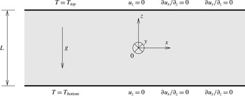
A horizontal fluid layer of thickness
 $L$
, in a uniform gravity field
 $\boldsymbol{g}=-g\boldsymbol{e}_{z}$
, is heated from below: the lower and upper boundaries are maintained at
 $T_{bottom}$
and
 $T_{top}$
, respectively. The fluid is a Newtonian fluid and obeys the Fourier law of heat conduction. Its dynamic viscosity
 $\unicode[STIX]{x1D707}$
and thermal conductivity
 $k$
are taken to be uniform, independent of pressure and temperature, for simplicity. The mechanical boundary conditions are stress-free, impermeable, on the upper and lower planar boundaries. The governing equations for convection consist of the equations of continuity, momentum conservation (Navier–Stokes with no bulk viscosity), entropy balance and an equation of state:
 $$\begin{eqnarray}\displaystyle & \displaystyle \frac{\unicode[STIX]{x2202}\unicode[STIX]{x1D70C}}{\unicode[STIX]{x2202}t}+\unicode[STIX]{x1D735}\boldsymbol{\cdot }(\unicode[STIX]{x1D70C}\boldsymbol{u})=0, & \displaystyle\end{eqnarray}$$
 $$\begin{eqnarray}\displaystyle & \displaystyle \unicode[STIX]{x1D70C}\frac{\text{D}\boldsymbol{u}}{\text{D}t}=-\unicode[STIX]{x1D735}p+\unicode[STIX]{x1D70C}\boldsymbol{g}+\unicode[STIX]{x1D707}\left(\unicode[STIX]{x1D6FB}^{2}\boldsymbol{u}+\frac{1}{3}\unicode[STIX]{x1D735}(\unicode[STIX]{x1D735}\boldsymbol{\cdot }\boldsymbol{u})\right), & \displaystyle\end{eqnarray}$$
 $$\begin{eqnarray}\displaystyle & \displaystyle \unicode[STIX]{x1D70C}c_{p}\frac{\text{D}T}{\text{D}t}-\unicode[STIX]{x1D6FC}T\frac{\text{D}p}{\text{D}t}=\dot{\unicode[STIX]{x1D750}}\boldsymbol{ : }\unicode[STIX]{x1D749}+k\unicode[STIX]{x1D6FB}^{2}T, & \displaystyle\end{eqnarray}$$
 $$\begin{eqnarray}\displaystyle & \displaystyle \unicode[STIX]{x1D70C}=\unicode[STIX]{x1D70C}(p,T), & \displaystyle\end{eqnarray}$$
where
 $t,\unicode[STIX]{x1D70C},\boldsymbol{u},p,T,c_{p},\unicode[STIX]{x1D6FC},\dot{\unicode[STIX]{x1D750}}$
and
 $\unicode[STIX]{x1D749}$
are the time, density, velocity vector, pressure, temperature, heat capacity at constant pressure, expansion coefficient, deformation rate tensor and stress tensor, respectively. A vertical coordinate axis
 $z$
is defined with its origin on the mid-plane of the layer (see figure 1). Horizontal coordinates
 $x$
and
 $y$
form an orthogonal unit reference frame. The boundary conditions associated with the governing equations are the following:
 $$\begin{eqnarray}\displaystyle u_{z}\left(z=\pm \frac{L}{2}\right)=0, & & \displaystyle\end{eqnarray}$$
 $$\begin{eqnarray}\displaystyle T\left(z=\frac{L}{2}\right)=T_{top},\quad T\left(z=-\frac{L}{2}\right)=T_{bottom}, & & \displaystyle\end{eqnarray}$$
 $$\begin{eqnarray}\displaystyle & \displaystyle \frac{\unicode[STIX]{x2202}u_{x}}{\unicode[STIX]{x2202}z}\left(z=\pm \frac{L}{2}\right)=0, & \displaystyle\end{eqnarray}$$
 $$\begin{eqnarray}\displaystyle & \displaystyle \frac{\unicode[STIX]{x2202}u_{y}}{\unicode[STIX]{x2202}z}\left(z=\pm \frac{L}{2}\right)=0. & \displaystyle\end{eqnarray}$$
The initial condition considered will be a quiescent state and will be described in § 4. The mass of fluid per horizontal unit surface area is set when the density of the base profile
 $\unicode[STIX]{x1D70C}_{0}$
is specified at
 $z=0$
.
Rayleigh–Bénard configuration, with imposed temperatures and tangential stress-free boundary conditions.

3 Dimensionless formulation
The dimensional quantities will be made dimensionless with the help of the quiescent base solution. The density, thermal expansion coefficient and specific heat capacity at constant pressure of the base solution at
 $z=0$
, i.e.
 $\unicode[STIX]{x1D70C}_{0}$
,
 $\unicode[STIX]{x1D6FC}_{0}$
and
 $c_{p0}$
respectively, will be the scales for density, thermal expansion coefficient and specific heat capacity at constant pressure, and
 $T_{0}=(T_{top}+T_{bottom})/2$
will be the scale for temperature. Pressure
 $p$
, velocity
 $\boldsymbol{u}$
, time
 $t$
and spatial coordinates
 $\boldsymbol{x}$
are made dimensionless using
 $\unicode[STIX]{x1D70C}_{0}gL$
,
 $k/(\unicode[STIX]{x1D70C}_{0}c_{p0}L)$
,
 $L^{2}\unicode[STIX]{x1D70C}_{0}c_{p0}/k$
and
 $L$
, respectively. The governing equations take the following dimensionless form:
 $$\begin{eqnarray}\displaystyle & \displaystyle \frac{\unicode[STIX]{x2202}\unicode[STIX]{x1D70C}}{\unicode[STIX]{x2202}t}+\unicode[STIX]{x1D735}\boldsymbol{\cdot }(\unicode[STIX]{x1D70C}\boldsymbol{u})=0, & \displaystyle\end{eqnarray}$$
 $$\begin{eqnarray}\displaystyle & \displaystyle Pr^{-1}\unicode[STIX]{x1D70C}\frac{\text{D}\boldsymbol{u}}{\text{D}t}=-Ra_{th}\unicode[STIX]{x1D735}p-Ra_{th}\unicode[STIX]{x1D70C}\boldsymbol{e}_{z}+\unicode[STIX]{x1D6FB}^{2}\boldsymbol{u}+\frac{1}{3}\unicode[STIX]{x1D735}(\unicode[STIX]{x1D735}\boldsymbol{\cdot }\boldsymbol{u}), & \displaystyle\end{eqnarray}$$
 $$\begin{eqnarray}\displaystyle & \displaystyle \unicode[STIX]{x1D70C}c_{p}\frac{\text{D}T}{\text{D}t}-{\mathcal{D}}\unicode[STIX]{x1D6FC}T\frac{\text{D}p}{\text{D}t}=\dot{\unicode[STIX]{x1D750}}\boldsymbol{ : }\unicode[STIX]{x1D749}+\unicode[STIX]{x1D6FB}^{2}T, & \displaystyle\end{eqnarray}$$
where
 $Pr=\unicode[STIX]{x1D707}c_{p0}/k$
is the Prandtl number,
 $Ra_{th}=\unicode[STIX]{x1D70C}_{0}^{2}gc_{p0}L^{3}/(\unicode[STIX]{x1D707}k)$
is called here the thermodynamic Rayleigh number and
 ${\mathcal{D}}=\unicode[STIX]{x1D6FC}_{0}gL/c_{p0}$
is the dissipation number. The thermal boundary conditions necessitate an additional dimensionless parameter and we choose the ratio of the temperature difference to the average temperature
 $a=2(T_{bottom}-T_{top})/(T_{bottom}+T_{top})$
, so that the boundary conditions (2.6) become
 $$\begin{eqnarray}T\left(z=\frac{1}{2}\right)=1-\frac{a}{2},\quad T\left(z=-\frac{1}{2}\right)=1+\frac{a}{2}.\end{eqnarray}$$
From our choice of dimensional scales, another dimensionless number is obtained from the product
 $\unicode[STIX]{x1D6FC}_{0}T_{0}$
. The equations of state will also be made dimensionless when they are considered in § 8. Depending on the equation of state, dimensionless parameters other than the four numbers listed above may or may not be necessary. We have not specified how the viscous dissipation term
 $\dot{\unicode[STIX]{x1D716}}:\unicode[STIX]{x1D70F}$
was made dimensionless because this term is quadratic in terms of velocity disturbances, hence will play no role in the linear stability analysis.
From this set of dimensionless numbers, it is possible to express the classical Rayleigh number,
 $Ra$
, as follows:
 $$\begin{eqnarray}Ra=Ra_{th}\unicode[STIX]{x1D6FC}_{0}(T_{bottom}-T_{top})=Ra_{th}\unicode[STIX]{x1D6FC}_{0}T_{0}a.\end{eqnarray}$$
4 Motionless base solution
The base solution is a pure conduction, hydrostatic state. The dynamic and thermal equations (3.2) and (3.3) lead to the following equations for
 $p_{b}$
,
 $\unicode[STIX]{x1D70C}_{b}$
and
 $T_{b}$
, the base pressure, density and temperature solutions, which are functions of
 $z$
only:
 $$\begin{eqnarray}\displaystyle & \displaystyle \frac{\text{d}p_{b}}{\text{d}z}=-\unicode[STIX]{x1D70C}_{b}, & \displaystyle\end{eqnarray}$$
 $$\begin{eqnarray}\displaystyle & \displaystyle \frac{\text{d}^{2}T_{b}}{\text{d}z^{2}}=0. & \displaystyle\end{eqnarray}$$
The boundary condition (3.4) for temperature needs to be satisfied. The conduction solution can be expressed as
 $$\begin{eqnarray}T_{b}=1-az.\end{eqnarray}$$
The opposite of the temperature gradient is
 $a$
and the bottom to top temperature ratio
 $T_{bottom}/T_{top}$
is
 $r=(2+a)/(2-a)$
.
5 Eigenvalue equations for infinitesimal disturbances
Infinitesimal disturbances, denoted by primes, are added to the base solution and the temporal linear stability is analysed. The governing equations are linearized around the base solution and the resulting problem can be written as
 $$\begin{eqnarray}\displaystyle & \displaystyle \frac{\unicode[STIX]{x2202}\unicode[STIX]{x1D70C}^{\prime }}{\unicode[STIX]{x2202}t}=-\unicode[STIX]{x1D735}\boldsymbol{\cdot }(\unicode[STIX]{x1D70C}_{b}\boldsymbol{u}^{\prime }), & \displaystyle\end{eqnarray}$$
 $$\begin{eqnarray}\displaystyle & \displaystyle Pr^{-1}\unicode[STIX]{x1D70C}_{b}\frac{\unicode[STIX]{x2202}\boldsymbol{u}^{\prime }}{\unicode[STIX]{x2202}t}=-Ra_{th}\unicode[STIX]{x1D735}p^{\prime }-Ra_{th}\unicode[STIX]{x1D70C}^{\prime }\boldsymbol{e}_{z}+\unicode[STIX]{x1D6FB}^{2}\boldsymbol{u}^{\prime }+\frac{1}{3}\unicode[STIX]{x1D735}(\unicode[STIX]{x1D735}\boldsymbol{\cdot }\boldsymbol{u}^{\prime }), & \displaystyle\end{eqnarray}$$
 $$\begin{eqnarray}\displaystyle & \displaystyle \unicode[STIX]{x1D70C}_{b}c_{pb}\frac{\unicode[STIX]{x2202}T^{\prime }}{\unicode[STIX]{x2202}t}-{\mathcal{D}}\unicode[STIX]{x1D6FC}_{b}T_{b}\frac{\unicode[STIX]{x2202}p^{\prime }}{\unicode[STIX]{x2202}t}=-\unicode[STIX]{x1D70C}_{b}c_{pb}u_{z}^{\prime }\frac{\text{d}T_{b}}{\text{d}z}+{\mathcal{D}}\unicode[STIX]{x1D6FC}_{b}T_{b}u_{z}^{\prime }\frac{\text{d}p_{b}}{\text{d}z}+\unicode[STIX]{x1D6FB}^{2}T^{\prime }, & \displaystyle\end{eqnarray}$$
where
 $c_{pb}$
and
 $\unicode[STIX]{x1D6FC}_{b}$
are the heat capacity and thermal expansivity along the base profile. The problem does not explicitly depend on time
 $t$
, nor on the horizontal directions
 $x$
and
 $y$
. Thus general solutions can be sought in the linear space of plane waves:
 $$\begin{eqnarray}T^{\prime }=\widetilde{T}(z)\exp (\unicode[STIX]{x1D70E}t+\text{i}k_{x}x+\text{i}k_{y}y),\end{eqnarray}$$
and so on for all variables, where
 $\unicode[STIX]{x1D70E}$
is the growth rate of the disturbance, and
 $k_{x}$
and
 $k_{y}$
its horizontal wavenumbers. As rotation along a vertical axis leaves the problem unchanged, we can restrict the analysis to
 $k_{y}=0$
without any loss of generality. Equations (5.1), (5.2) and (5.3) are then changed into the following eigenvalue problem:
 $$\begin{eqnarray}\displaystyle & \displaystyle \unicode[STIX]{x1D70E}\widetilde{\unicode[STIX]{x1D70C}}=-\text{i}k_{x}\unicode[STIX]{x1D70C}_{b}\widetilde{u}_{x}-\unicode[STIX]{x1D70C}_{b}\frac{\text{d}\widetilde{u}_{z}}{\text{d}z}-\frac{\text{d}\unicode[STIX]{x1D70C}_{b}}{\text{d}z}\widetilde{u}_{z}, & \displaystyle\end{eqnarray}$$
 $$\begin{eqnarray}\displaystyle & \displaystyle \unicode[STIX]{x1D70E}Pr^{-1}\unicode[STIX]{x1D70C}_{b}\widetilde{u}_{x}=-Ra_{th}\text{i}k_{x}\widetilde{p}-\frac{4}{3}k_{x}^{2}\widetilde{u}_{x}+\frac{\text{i}k_{x}}{3}\frac{\text{d}\widetilde{u}_{z}}{\text{d}z}+\frac{\text{d}^{2}\widetilde{u}_{x}}{\text{d}z^{2}}, & \displaystyle\end{eqnarray}$$
 $$\begin{eqnarray}\displaystyle & \displaystyle \unicode[STIX]{x1D70E}Pr^{-1}\unicode[STIX]{x1D70C}_{b}\widetilde{u}_{z}=-Ra_{th}\frac{\text{d}\widetilde{p}}{\text{d}z}-Ra_{th}\widetilde{\unicode[STIX]{x1D70C}}-k_{x}^{2}\widetilde{u}_{z}+\frac{\text{i}k_{x}}{3}\frac{\text{d}\widetilde{u}_{x}}{\text{d}z}+\frac{4}{3}\frac{\text{d}^{2}\widetilde{u}_{z}}{\text{d}z^{2}}, & \displaystyle\end{eqnarray}$$
 $$\begin{eqnarray}\displaystyle & \displaystyle \unicode[STIX]{x1D70E}\unicode[STIX]{x1D70C}_{b}c_{pb}\widetilde{T}-\unicode[STIX]{x1D70E}{\mathcal{D}}\unicode[STIX]{x1D6FC}_{b}T_{b}\widetilde{p}=-\unicode[STIX]{x1D70C}_{b}c_{pb}\widetilde{u}_{z}\frac{\text{d}T_{b}}{\text{d}z}+{\mathcal{D}}\unicode[STIX]{x1D6FC}_{b}T_{b}\widetilde{u}_{z}\frac{\text{d}p_{b}}{\text{d}z}-k_{x}^{2}\widetilde{T}+\frac{\text{d}^{2}\widetilde{T}}{\text{d}z^{2}}. & \displaystyle\end{eqnarray}$$
Finally, the density disturbance
 $\widetilde{\unicode[STIX]{x1D70C}}$
is expanded linearly in terms of temperature
 $\widetilde{T}$
and pressure
 $\widetilde{p}$
disturbances in (5.7) when a particular equation of state will be considered:
 $$\begin{eqnarray}\widetilde{\unicode[STIX]{x1D70C}}=\left.\frac{\unicode[STIX]{x2202}\unicode[STIX]{x1D70C}}{\unicode[STIX]{x2202}T}\right|_{p}\widetilde{T}+\left.\frac{\unicode[STIX]{x2202}\unicode[STIX]{x1D70C}}{\unicode[STIX]{x2202}p}\right|_{T}\widetilde{p}.\end{eqnarray}$$
Our objective is to obtain the critical value of the thermodynamic Rayleigh number
 $Ra_{th}$
as a function of the other dimensionless numbers. We restrict our analysis to the critical threshold,
 $\text{Re}(\unicode[STIX]{x1D70E})=0$
. The eigenvalue problem is not self-adjoint in general, unlike the classical Boussinesq problem; however, the imaginary part of the critical eigenvalue is always found to be zero in our numerical calculations. The first instability takes the form of a stationary pattern, not a travelling wave. A consequence is that the Prandtl number is irrelevant in our study, since it appears only as the product
 $\unicode[STIX]{x1D70E}\,Pr^{-1}$
in the eigenvalue problem, in (5.6) and (5.7).
The eigenvalue problem is solved and the critical Rayleigh number for neutral stability is obtained. The method is that of Chebyshev collocation expansion and we use the differentiation matrices provided by the DIFFMAT suite (Weideman & Reddy Reference Weideman and Reddy2000). The computations are run in GNU Octave on a laptop. The results of the stability analysis will be presented in terms of the superadiabatic Rayleigh number, defined as
 $$\begin{eqnarray}Ra_{SA}=Ra_{th}\unicode[STIX]{x1D6FC}_{0}T_{0}\unicode[STIX]{x0394}T_{SA},\end{eqnarray}$$
where
 $\unicode[STIX]{x0394}T_{SA}$
denotes the dimensionless superadiabatic temperature difference. The imposed total dimensionless temperature difference is
 $a$
, but there are actually different possibilities to define the dimensionless adiabatic temperature difference. Here, we simply take the product of the adiabatic gradient
 $\unicode[STIX]{x1D6FC}gT/c_{p}$
at
 $z=0$
(at conditions
 $\unicode[STIX]{x1D70C}=\unicode[STIX]{x1D70C}_{0}$
and
 $T=T_{0}$
) with the thickness
 $L$
, which provides a dimensionless adiabatic temperature difference equal to
 ${\mathcal{D}}$
, so that we define
 $\unicode[STIX]{x0394}T_{SA}$
as
 $$\begin{eqnarray}\unicode[STIX]{x0394}T_{SA}=a-{\mathcal{D}}.\end{eqnarray}$$
We could have taken the total temperature difference calculated across a complete adiabat, instead. Then, again, different choices of adiabatic profiles are possible: the profile passing through the same conditions as the conduction profile at
 $z=0$
, the profile with the same total mass, …. Each choice of an adiabatic temperature profile leads to a different value of the superadiabatic jump. Because a difference in
 $z^{2}$
in the adiabatic temperature makes no contribution between
 $z=-1/2$
and
 $1/2$
, other definitions would have led to temperature jumps departing from (5.11) by a cubic expression in terms of
 $a$
and
 ${\mathcal{D}}$
. Anticipating the rest of the analysis, this would change the departure of the critical Rayleigh number from the Boussinesq limit by quadratic terms in
 $a$
and
 ${\mathcal{D}}$
. This is also the order of departure of the critical Rayleigh number from the Boussinesq limit that we compute in the following. However, differences of superadiabatic Rayleigh numbers from different approximations (exact, quasi-ALA and quasi-Boussinesq) will not depend on that choice of superadiabatic temperature difference, as its contributions will essentially cancel out.
6 An approximate analysis with two modes
We assume that the imaginary part of the eigenvalue is zero at critical conditions,
 $\unicode[STIX]{x1D70E}=0$
, and (5.5), (5.6), (5.7) and (5.8) take the form:
 $$\begin{eqnarray}\displaystyle & \displaystyle 0=-\text{i}k_{x}\unicode[STIX]{x1D70C}_{b}\widetilde{u}_{x}-\unicode[STIX]{x1D70C}_{b}\text{D}\widetilde{u}_{z}-\unicode[STIX]{x1D70C}_{b}^{\prime }\widetilde{u}_{z}, & \displaystyle\end{eqnarray}$$
 $$\begin{eqnarray}\displaystyle & \displaystyle 0=-Ra_{th}\text{i}k_{x}\widetilde{p}-\frac{4}{3}k_{x}^{2}\widetilde{u}_{x}+\frac{\text{i}k_{x}}{3}\text{D}\widetilde{u}_{z}+\text{D}^{2}\widetilde{u}_{x}, & \displaystyle\end{eqnarray}$$
 $$\begin{eqnarray}\displaystyle & \displaystyle 0=-Ra_{th}\text{D}\widetilde{p}-Ra_{th}\left.\frac{\unicode[STIX]{x2202}\unicode[STIX]{x1D70C}}{\unicode[STIX]{x2202}T}\right|_{P}\widetilde{T}-Ra_{th}\left.\frac{\unicode[STIX]{x2202}\unicode[STIX]{x1D70C}}{\unicode[STIX]{x2202}p}\right|_{T}\widetilde{p}-k_{x}^{2}\widetilde{u}_{z}+\frac{\text{i}k_{x}}{3}\text{D}\widetilde{u}_{x}+\frac{4}{3}\text{D}^{2}\widetilde{u}_{z}, & \displaystyle\end{eqnarray}$$
 $$\begin{eqnarray}\displaystyle & \displaystyle 0=(-\unicode[STIX]{x1D70C}_{b}c_{pb}T_{b}^{\prime }+{\mathcal{D}}\unicode[STIX]{x1D6FC}_{b}T_{b}p_{b}^{\prime })\widetilde{u}_{z}-k_{x}^{2}\widetilde{T}+\text{D}^{2}\widetilde{T}. & \displaystyle\end{eqnarray}$$
The primes denotes
 $z$
derivatives of the base solution profiles, while the symbol
 $\text{D}$
(respectively
 $\text{D}^{2}$
,
 $\text{D}^{3}$
, …) denotes
 $z$
derivatives (respectively second, third, … derivatives) of the perturbation variables. Then
 $\widetilde{u}_{x}$
is substituted using the first equation, and a function of
 $z$
is introduced,
 $g(z)=(\unicode[STIX]{x1D70C}_{b}c_{pb}T_{b}^{\prime }-{\mathcal{D}}\unicode[STIX]{x1D6FC}_{b}T_{b}p_{b}^{\prime })^{-1}$
, in order to simplify the fourth equation, which takes the form
 $\widetilde{u}_{z}=g(z)(\text{D}^{2}-k_{x}^{2})\widetilde{T}$
. Note that
 $g(0)=(T_{b}^{\prime }(0)-{\mathcal{D}}p_{b}^{\prime }(0))^{-1}=(-a+{\mathcal{D}})^{-1}$
. The pressure term is substituted using the second equation into the third one and
 $\widetilde{u}_{z}$
is expressed in terms of
 $\widetilde{T}$
using the fourth equation. Finally, we get a single differential equation for the perturbation
 $\widetilde{T}$
:
 $$\begin{eqnarray}\displaystyle 0 & = & \displaystyle -(\text{D}^{2}-k_{x}^{2})\text{D}\left(\text{D}+\frac{\unicode[STIX]{x1D70C}_{b}^{\prime }}{\unicode[STIX]{x1D70C}_{b}}\right)g(\text{D}^{2}-k_{x}^{2})\widetilde{T}-k_{x}^{2}Ra_{th}\left.\frac{\unicode[STIX]{x2202}\unicode[STIX]{x1D70C}}{\unicode[STIX]{x2202}T}\right|_{p}\widetilde{T}+k_{x}^{2}(\text{D}^{2}-k_{x}^{2})g(\text{D}^{2}-k_{x}^{2})\widetilde{T}\nonumber\\ \displaystyle & & \displaystyle +\,\left.\frac{\unicode[STIX]{x2202}\unicode[STIX]{x1D70C}}{\unicode[STIX]{x2202}p}\right|_{T}\left[\frac{1}{3}k_{x}^{2}\frac{\unicode[STIX]{x1D70C}_{b}^{\prime }}{\unicode[STIX]{x1D70C}_{b}}g(\text{D}^{2}-k_{x}^{2})-(\text{D}^{2}-k_{x}^{2})\left(\text{D}+\frac{\unicode[STIX]{x1D70C}_{b}^{\prime }}{\unicode[STIX]{x1D70C}_{b}}\right)g(\text{D}^{2}-k_{x}^{2})\right]\widetilde{T}.\end{eqnarray}$$
We now introduce
 $f(z)=\unicode[STIX]{x0394}T_{SA}\,g(z)=\unicode[STIX]{x0394}T_{SA}/(\unicode[STIX]{x1D70C}_{b}c_{pb}T_{b}^{\prime }-{\mathcal{D}}\unicode[STIX]{x1D6FC}_{b}T_{b}p_{b}^{\prime })$
, where the superadiabatic temperature difference
 $\unicode[STIX]{x0394}T_{SA}$
has been defined in (5.11). As a consequence of the choice of superadiabatic temperature difference (5.11), we obtain the value of
 $f$
at
 $z=0$
:
 $$\begin{eqnarray}f|_{0}=-1.\end{eqnarray}$$
The critical disturbance equation can be written:
 $$\begin{eqnarray}\displaystyle 0 & = & \displaystyle -(\text{D}^{2}-k_{x}^{2})\text{D}\left(\text{D}+\frac{\unicode[STIX]{x1D70C}_{b}^{\prime }}{\unicode[STIX]{x1D70C}_{b}}\right)f(\text{D}^{2}-k_{x}^{2})\widetilde{T}\nonumber\\ \displaystyle & & \displaystyle -\,\frac{k_{x}^{2}}{\unicode[STIX]{x1D6FC}_{0}T_{0}}Ra_{SA}\left.\frac{\unicode[STIX]{x2202}\unicode[STIX]{x1D70C}}{\unicode[STIX]{x2202}T}\right|_{p}\widetilde{T}+k_{x}^{2}(\text{D}^{2}-k_{x}^{2})f(\text{D}^{2}-k_{x}^{2})\widetilde{T}\nonumber\\ \displaystyle & & \displaystyle +\,\left.\frac{\unicode[STIX]{x2202}\unicode[STIX]{x1D70C}}{\unicode[STIX]{x2202}p}\right|_{T}\left[\frac{1}{3}k_{x}^{2}\frac{\unicode[STIX]{x1D70C}_{b}^{\prime }}{\unicode[STIX]{x1D70C}_{b}}f(\text{D}^{2}-k_{x}^{2})-(\text{D}^{2}-k_{x}^{2})\left(\text{D}+\frac{\unicode[STIX]{x1D70C}_{b}^{\prime }}{\unicode[STIX]{x1D70C}_{b}}\right)f(\text{D}^{2}-k_{x}^{2})\right]\widetilde{T}.\end{eqnarray}$$
This equation depends on several functions of
 $z$
, computed along the base profile, namely
 $f$
,
 $\unicode[STIX]{x1D70C}_{b}^{\prime }/\unicode[STIX]{x1D70C}_{b}$
,
 $(\unicode[STIX]{x2202}\unicode[STIX]{x1D70C}/\unicode[STIX]{x2202}T)|_{p}$
and
 $(\unicode[STIX]{x2202}\unicode[STIX]{x1D70C}/\unicode[STIX]{x2202}p)|_{T}$
, all depending on the equation of state considered and on the dimensionless governing parameters
 $a$
and
 ${\mathcal{D}}$
. In the limit of vanishing temperature difference across the convecting layer,
 $a\ll 1$
, the temperature becomes nearly homogeneous
 $T\simeq T_{0}$
. The variation of density with pressure at
 $z=0$
,
 $(\unicode[STIX]{x2202}\unicode[STIX]{x1D70C}/\unicode[STIX]{x2202}p)|_{T0}=\unicode[STIX]{x1D70C}_{0}/K_{T0}$
(
 $K_{T0}$
is the isothermal incompressibility at
 $z=0$
) can be expressed in the following dimensionless form:
 $$\begin{eqnarray}\left.\frac{\unicode[STIX]{x2202}\unicode[STIX]{x1D70C}}{\unicode[STIX]{x2202}p}\right|_{T0}=\widetilde{{\mathcal{D}}}\unicode[STIX]{x1D6FC}_{0}T_{0},\end{eqnarray}$$
using the general Mayer’s relation
 $$\begin{eqnarray}c_{p}-c_{v}=\frac{\unicode[STIX]{x1D6FC}^{2}K_{T}T}{\unicode[STIX]{x1D70C}},\end{eqnarray}$$
where
 $c_{v}$
is the heat capacity at constant volume, and defining, for the sake of brevity,
 $$\begin{eqnarray}\widetilde{{\mathcal{D}}}=\frac{{\mathcal{D}}}{1-\unicode[STIX]{x1D6FE}_{0}^{-1}},\quad \unicode[STIX]{x1D6FE}_{0}=\frac{c_{p0}}{c_{v0}}\quad \text{and}\quad \hat{\unicode[STIX]{x1D6FC}}=\unicode[STIX]{x1D6FC}_{0}T_{0}.\end{eqnarray}$$
Note that
 $\widetilde{{\mathcal{D}}}$
can also be written as
 $$\begin{eqnarray}\widetilde{{\mathcal{D}}}=\frac{1}{\hat{\unicode[STIX]{x1D6FC}}}\frac{\unicode[STIX]{x1D70C}_{0}gL}{K_{T0}}.\end{eqnarray}$$
The parameter
 $\widetilde{{\mathcal{D}}}$
is therefore the ratio of compressible to thermal effects. There is no surprise in that it will be the central parameter to discuss the compressible effects in thermal convection. In the limit of a vanishing compressibility (
 $\widetilde{{\mathcal{D}}}\ll 1$
or
 ${\mathcal{D}}\ll 1$
), the base density becomes independent of pressure. Therefore, when both
 $a$
and
 ${\mathcal{D}}$
are small, the temperature becomes constant, the density independent of pressure and
 $f=-1$
,
 $\unicode[STIX]{x1D70C}_{b}^{\prime }/\unicode[STIX]{x1D70C}_{b}=0$
,
 $(\unicode[STIX]{x2202}\unicode[STIX]{x1D70C}/\unicode[STIX]{x2202}T)|_{p}=-\unicode[STIX]{x1D6FC}_{0}T_{0}$
and
 $(\unicode[STIX]{x2202}\unicode[STIX]{x1D70C}/\unicode[STIX]{x2202}p)|_{T}=0$
, and the critical equation becomes the well-known dispersion relation for Rayleigh–Bénard stability:
 $$\begin{eqnarray}(\text{D}^{2}-k_{x}^{2})^{3}\widetilde{T}+k_{x}^{2}Ra_{SA}\widetilde{T}=0,\end{eqnarray}$$
in accordance with Jeffreys’ analysis (Jeffreys Reference Jeffreys1930). Under the additional assumption of a negligible adiabatic gradient compared to the imposed temperature difference,
 ${\mathcal{D}}\ll a$
, the superadiabatic Rayleigh number
 $Ra_{SA}$
is replaced by the classical Rayleigh number (3.5) in (6.12), which then becomes the exact equation solved by Rayleigh (Reference Rayleigh1916) in the Boussinesq approximation. The thermal perturbation
 $\widetilde{T}$
satisfies
 $\widetilde{T}=0$
in
 $z=\pm 1/2$
(fixed temperatures),
 $\text{D}^{2}\widetilde{T}=0$
(
 $\widetilde{u}_{z}=0$
) and
 $\text{D}^{4}\widetilde{T}=0$
(no-stress conditions). It has non-zero solutions for a minimal value of
 $Ra_{SA}=27\unicode[STIX]{x03C0}^{4}/4$
and a corresponding wavenumber
 $k_{x}=\unicode[STIX]{x03C0}/\sqrt{2}$
. The corresponding eigenvector is a cosine function
 $\cos (\unicode[STIX]{x03C0}z)$
.
Now, for a finite temperature gradient
 $a$
or dissipation number
 ${\mathcal{D}}$
, the functions
 $f$
and
 $(\unicode[STIX]{x2202}\unicode[STIX]{x1D70C}/\unicode[STIX]{x2202}T)|_{p}$
, have some
 $z$
dependence and the functions
 $\unicode[STIX]{x1D70C}_{b}^{\prime }/\unicode[STIX]{x1D70C}_{b}$
and
 $(\unicode[STIX]{x2202}\unicode[STIX]{x1D70C}/\unicode[STIX]{x2202}p)|_{T}$
are not zero. As a consequence, when an even function of
 $z$
is initially considered for the temperature eigenvector, there are odd contributions generated in (6.7). Hence, the eigenvectors must be a combination of at least an even and an odd contribution. Hence, we decided to expand the eigenmodes as
 $$\begin{eqnarray}\widetilde{T}=\cos (\unicode[STIX]{x03C0}z)+\unicode[STIX]{x1D716}\sin (2\unicode[STIX]{x03C0}z).\end{eqnarray}$$
The motivation for this particular choice
 $\sin (2\unicode[STIX]{x03C0}z)$
of odd function of
 $z$
is that it satisfies the boundary conditions and that it is the second least dissipative harmonic mode after
 $\cos (\unicode[STIX]{x03C0}z)$
. In addition, we have checked on some eigenvectors obtained using Chebyshev expansion that they could be written as the sum of two such modes (6.13) with negligible residuals (see § 8 and figure 9).
We wish to achieve a second-order accuracy, in the base temperature gradient
 $a$
and in the dissipation number
 ${\mathcal{D}}$
, so that we can evaluate the change in critical Rayleigh number to a similar degree. We thus expand the functions of
 $z$
related to the base profile
 $f$
,
 $\unicode[STIX]{x1D70C}_{b}^{\prime }/\unicode[STIX]{x1D70C}_{b}$
,
 $(\unicode[STIX]{x2202}\unicode[STIX]{x1D70C}/\unicode[STIX]{x2202}T)|_{p}$
and
 $(\unicode[STIX]{x2202}\unicode[STIX]{x1D70C}/\unicode[STIX]{x2202}p)|_{T}$
in Taylor expansions of degree two, for instance:
 $$\begin{eqnarray}f(z)=f_{0}+\left.\frac{\text{d}f}{\text{d}z}\right|_{0}z+\frac{1}{2}\left.\frac{\text{d}^{2}f}{\text{d}z^{2}}\right|_{0}z^{2},\end{eqnarray}$$
and similarly for the others. The introduction of the expansions of the form (6.14) and (6.13) into the critical equation (6.7) generates terms that are products of trigonometric functions and powers of
 $z$
. We project these functions back on the two chosen modes
 $\cos (\unicode[STIX]{x03C0}z)$
and
 $\sin (2\unicode[STIX]{x03C0}z)$
. The projection is that associated with the
 $L^{2}$
functional space on
 $[-1/2,1/2]$
(see table 1). The change in the reference profiles due to the dissipation parameter
 ${\mathcal{D}}$
and finite temperature gradient
 $a$
affects not only
 $\unicode[STIX]{x1D716}$
but also the critical Rayleigh number by a quantity
 $\text{d}Ra_{SA}$
,
 $$\begin{eqnarray}Ra_{SA}={\textstyle \frac{27}{4}}\unicode[STIX]{x03C0}^{4}+\text{d}Ra_{SA}.\end{eqnarray}$$
For any equation of state from which the stable basic state can be computed and Taylor-expanded (as in (6.14)), our eigenmodes (6.13) introduced into the critical equation (6.7) lead to two equations (i.e. the terms in
 $\cos (\unicode[STIX]{x03C0}z)$
and
 $\sin (2\unicode[STIX]{x03C0}z)$
) whose solutions are the eigenmode amplitude
 $\unicode[STIX]{x1D716}$
(from the
 $\sin (2\unicode[STIX]{x03C0}z)$
part) and the perturbation of the critical Rayleigh number
 $\text{d}Ra_{SA}$
(from the
 $\cos (\unicode[STIX]{x03C0}z)$
part). A close look at the equations indicates that
 $\unicode[STIX]{x1D716}$
depends linearly on the parameters describing the distance of the problem from the classical Boussinesq problem (mainly
 $a$
and
 ${\mathcal{D}}$
, the temperature gradient and dissipation number) while
 $\text{d}Ra_{SA}$
is only affected by terms of order two. Similarly the horizontal wavenumber
 $k_{x}$
is also affected by terms of order two. Moreover, because the critical Rayleigh number is also such that
 $\text{d}Ra_{SA}/\text{d}k_{x}=0$
(minimal Rayleigh number over wavenumbers), the quadratic disturbance of
 $k_{x}$
does not affect the evaluation of the quadratic disturbance of
 $Ra_{SA}$
. It is hence correct to use a constant value
 $k_{x}=\unicode[STIX]{x03C0}/\sqrt{2}$
for this analysis.
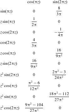
Projection coefficients of some functions on the modes
 $\cos (\unicode[STIX]{x03C0}z)$
and
 $\sin (2\unicode[STIX]{x03C0}z)$
.

Let us now provide some details on how the equations for
 $\unicode[STIX]{x1D716}$
and
 $\text{d}Ra_{SA}$
are derived. We introduce
 $\widetilde{u}=f(\text{D}^{2}-k_{x}^{2})\widetilde{T}$
,
 $a-{\mathcal{D}}$
times the vertical velocity component
 $\widetilde{u}_{z}$
, and
 $\widetilde{v}=\text{D}(\text{D}+\unicode[STIX]{x1D70C}_{b}^{\prime }/\unicode[STIX]{x1D70C}_{b})\widetilde{u}$
, which is
 $\text{i}(a-{\mathcal{D}})/k_{x}$
times the
 $z$
derivative of the horizontal velocity component (from (6.1)). Using variables
 $\widetilde{T}$
,
 $\widetilde{u}$
and
 $\widetilde{v}$
, the critical equation (6.7) takes the form:
 $$\begin{eqnarray}0=-(\text{D}^{2}-k_{x}^{2})\widetilde{v}-\frac{k_{x}^{2}}{\unicode[STIX]{x1D6FC}_{0}T_{0}}Ra_{SA}\!\left.\frac{\unicode[STIX]{x2202}\unicode[STIX]{x1D70C}}{\unicode[STIX]{x2202}T}\right|_{p}\widetilde{T}+k_{x}^{2}(\text{D}^{2}-k_{x}^{2})\widetilde{u}+\!\left.\frac{\unicode[STIX]{x2202}\unicode[STIX]{x1D70C}}{\unicode[STIX]{x2202}p}\right|_{T}\left[\frac{4}{3}k_{x}^{2}\frac{\unicode[STIX]{x1D70C}_{b}^{\prime }}{\unicode[STIX]{x1D70C}_{b}}\widetilde{u}-\text{D}\widetilde{v}+k_{x}^{2}\text{D}\widetilde{u}\right]\!.\end{eqnarray}$$
Both
 $\widetilde{u}$
and
 $\widetilde{v}$
satisfy the same boundary conditions as
 $\widetilde{T}$
(zero in
 $z=\pm 1/2$
) so that they are also projected on the same modes defined in (6.13):
 $$\begin{eqnarray}\displaystyle & \displaystyle \widetilde{u}=U_{c}\cos (\unicode[STIX]{x03C0}z)+U_{s}\sin (2\unicode[STIX]{x03C0}z), & \displaystyle\end{eqnarray}$$
 $$\begin{eqnarray}\displaystyle & \displaystyle \widetilde{v}=V_{c}\cos (\unicode[STIX]{x03C0}z)+V_{s}\sin (2\unicode[STIX]{x03C0}z). & \displaystyle\end{eqnarray}$$
From the definition
 $\widetilde{u}=f(\text{D}^{2}-k_{x}^{2})\widetilde{T}$
, we have
 $$\begin{eqnarray}\displaystyle & \displaystyle U_{c}=-\frac{3\unicode[STIX]{x03C0}^{2}}{2}f_{0}-8\unicode[STIX]{x1D716}\left.\frac{\text{d}f}{\text{d}z}\right|_{0}+\left(-\frac{\unicode[STIX]{x03C0}^{2}}{16}+\frac{3}{8}\right)\left.\frac{\text{d}^{2}f}{\text{d}z^{2}}\right|_{0}, & \displaystyle\end{eqnarray}$$
 $$\begin{eqnarray}\displaystyle & \displaystyle U_{s}=-9\frac{\unicode[STIX]{x03C0}^{2}}{2}\unicode[STIX]{x1D716}f_{0}-\frac{8}{3}\left.\frac{\text{d}f}{\text{d}z}\right|_{0}, & \displaystyle\end{eqnarray}$$
where the projections determined in table 1 have been used. Using Maxima, software for formal manipulations, we shall obtain the Taylor coefficients for
 $f$
and other quantities, once an equation of state is specified. Next, from
 $\widetilde{v}=\text{D}(\text{D}+\unicode[STIX]{x1D70C}_{b}^{\prime }/\unicode[STIX]{x1D70C}_{b})\widetilde{u}$
, and using table 1 again, we obtain:
 $$\begin{eqnarray}\displaystyle & \displaystyle V_{c}=\left(-\unicode[STIX]{x03C0}^{2}+\frac{1}{2}\left.\frac{\text{d}(\unicode[STIX]{x1D70C}_{b}^{\prime }/\unicode[STIX]{x1D70C}_{b})}{\text{d}z}\right|_{0}\right)U_{c}+\frac{8}{3}\left.\frac{\unicode[STIX]{x1D70C}_{b}^{\prime }}{\unicode[STIX]{x1D70C}_{b}}\right|_{0}U_{s}, & \displaystyle\end{eqnarray}$$
 $$\begin{eqnarray}\displaystyle & \displaystyle V_{s}=-4\unicode[STIX]{x03C0}^{2}U_{s}-\frac{8}{3}\left.\frac{\unicode[STIX]{x1D70C}_{b}^{\prime }}{\unicode[STIX]{x1D70C}_{b}}\right|_{0}U_{c}. & \displaystyle\end{eqnarray}$$
Before we can write (6.16) using our two base functions, we need to define two auxiliary variables with the same zero boundary conditions as
 $\widetilde{T}$
in
 $z=\pm 1/2$
:
 $$\begin{eqnarray}\displaystyle & \displaystyle \left.\frac{\unicode[STIX]{x2202}\unicode[STIX]{x1D70C}}{\unicode[STIX]{x2202}T}\right|_{p}\widetilde{T}=A_{c}\cos (\unicode[STIX]{x03C0}z)+A_{s}\sin (2\unicode[STIX]{x03C0}z), & \displaystyle\end{eqnarray}$$
 $$\begin{eqnarray}\displaystyle & \displaystyle \frac{\unicode[STIX]{x1D70C}_{b}^{\prime }}{\unicode[STIX]{x1D70C}_{b}}\widetilde{u}=B_{c}\cos (\unicode[STIX]{x03C0}z)+B_{s}\sin (2\unicode[STIX]{x03C0}z), & \displaystyle\end{eqnarray}$$
with coefficients
 $$\begin{eqnarray}\displaystyle & \displaystyle A_{c}=-\hat{\unicode[STIX]{x1D6FC}}+\left(\frac{1}{24}-\frac{1}{4\unicode[STIX]{x03C0}^{2}}\right)\left.\frac{\text{d}^{2}(\unicode[STIX]{x2202}\unicode[STIX]{x1D70C}/\unicode[STIX]{x2202}T)|_{p}}{\text{d}z^{2}}\right|_{0}+\frac{16}{9\unicode[STIX]{x03C0}^{2}}\left.\frac{\text{d}(\unicode[STIX]{x2202}\unicode[STIX]{x1D70C}/\unicode[STIX]{x2202}T)|_{p}}{\text{d}z}\right|_{0}\unicode[STIX]{x1D716}, & \displaystyle\end{eqnarray}$$
 $$\begin{eqnarray}\displaystyle & \displaystyle A_{s}=\frac{16}{9\unicode[STIX]{x03C0}^{2}}\left.\frac{\text{d}(\unicode[STIX]{x2202}\unicode[STIX]{x1D70C}/\unicode[STIX]{x2202}T)|_{p}}{\text{d}z}\right|_{0}-\hat{\unicode[STIX]{x1D6FC}}\unicode[STIX]{x1D716}, & \displaystyle\end{eqnarray}$$
 $$\begin{eqnarray}\displaystyle & \displaystyle B_{c}=\left.\frac{\unicode[STIX]{x1D70C}_{b}^{\prime }}{\unicode[STIX]{x1D70C}_{b}}\right|_{0}U_{c}+\frac{16}{9\unicode[STIX]{x03C0}^{2}}\left.\frac{\text{d}(\unicode[STIX]{x1D70C}_{b}^{\prime }/\unicode[STIX]{x1D70C}_{b})}{\text{d}z}\right|_{0}U_{s}, & \displaystyle\end{eqnarray}$$
 $$\begin{eqnarray}\displaystyle & \displaystyle B_{s}=\left.\frac{\unicode[STIX]{x1D70C}_{b}^{\prime }}{\unicode[STIX]{x1D70C}_{b}}\right|_{0}U_{s}+\frac{16}{9\unicode[STIX]{x03C0}^{2}}\left.\frac{\text{d}(\unicode[STIX]{x1D70C}_{b}^{\prime }/\unicode[STIX]{x1D70C}_{b})}{\text{d}z}\right|_{0}U_{c}, & \displaystyle\end{eqnarray}$$
where we have used
 $(\unicode[STIX]{x2202}\unicode[STIX]{x1D70C}/\unicode[STIX]{x2202}T)|_{p0}=-\hat{\unicode[STIX]{x1D6FC}}$
. We can now write the projection of (6.16) on
 $\cos (\unicode[STIX]{x03C0}z)$
and
 $\sin (2\unicode[STIX]{x03C0}z)$
keeping only the terms of appropriate order:
 $$\begin{eqnarray}\displaystyle & & \displaystyle \frac{3}{2}\unicode[STIX]{x03C0}^{2}V_{c}-\frac{\unicode[STIX]{x03C0}^{2}}{2\hat{\unicode[STIX]{x1D6FC}}}\left(\frac{27\unicode[STIX]{x03C0}^{4}}{4}+\text{d}Ra_{SA}\right)A_{c}-\frac{3\unicode[STIX]{x03C0}^{4}}{4}U_{c}+\left.\frac{\unicode[STIX]{x2202}\unicode[STIX]{x1D70C}}{\unicode[STIX]{x2202}p}\right|_{T0}\left[\frac{2\unicode[STIX]{x03C0}^{2}}{3}B_{c}-\frac{8}{3}V_{s}+\frac{4\unicode[STIX]{x03C0}^{2}}{3}U_{s}\right]\nonumber\\ \displaystyle & & \displaystyle \quad +\,\left.\frac{\text{d}(\unicode[STIX]{x2202}\unicode[STIX]{x1D70C}/\unicode[STIX]{x2202}p)|_{T}}{\text{d}z}\right|_{0}\left[\frac{1}{2}V_{c}-\frac{\unicode[STIX]{x03C0}^{2}}{4}U_{c}\right]=0,\end{eqnarray}$$
 $$\begin{eqnarray}\displaystyle \frac{9}{2}\unicode[STIX]{x03C0}^{2}V_{s}-\frac{\unicode[STIX]{x03C0}^{2}}{2\hat{\unicode[STIX]{x1D6FC}}}\frac{27\unicode[STIX]{x03C0}^{4}}{4}A_{s}-\frac{9\unicode[STIX]{x03C0}^{4}}{4}U_{s}+\left.\frac{\unicode[STIX]{x2202}\unicode[STIX]{x1D70C}}{\unicode[STIX]{x2202}p}\right|_{T0}\left[\frac{8}{3}V_{c}-\frac{4\unicode[STIX]{x03C0}^{2}}{3}U_{c}\right]=0. & & \displaystyle\end{eqnarray}$$
Equation (6.30) is used to determine the coefficient
 $\unicode[STIX]{x1D716}$
(see 6.13). This coefficient
 $\unicode[STIX]{x1D716}$
depends linearly on the parameters describing the distance of the problem from the classical Boussinesq problem,
 $a$
and
 ${\mathcal{D}}$
, the temperature gradient and dissipation number. Equation (6.29) is then solved to obtain
 $\text{d}Ra_{SA}$
, the change in critical Rayleigh number compared to the classical critical Rayleigh number
 $27\unicode[STIX]{x03C0}^{4}/4$
for no-stress boundary conditions. This change is thus quadratic in
 $a$
and
 ${\mathcal{D}}$
: the terms of order zero cancel out (Boussinesq limit), the terms of order one are found in (6.30) used to determine the coefficient
 $\unicode[STIX]{x1D716}$
of the
 $\sin (2\unicode[STIX]{x03C0}z)$
mode, and the terms of order two balance
 $\text{d}Ra_{SA}$
in (6.29), with
 $A_{c}$
containing a term of order zero in
 $a$
and
 ${\mathcal{D}}$
.
Equation (6.30) and then (6.29) are solved explicitly in terms of the quantities
 $f$
,
 $\text{d}f/\text{d}z$
,
 $\text{d}^{2}f/\text{d}z^{2}$
,
 $\unicode[STIX]{x1D70C}_{b}^{\prime }/\unicode[STIX]{x1D70C}_{b}$
,
 $\text{d}(\unicode[STIX]{x1D70C}_{b}^{\prime }/\unicode[STIX]{x1D70C}_{b})/\text{d}z$
,
 $(\unicode[STIX]{x2202}\unicode[STIX]{x1D70C}/\unicode[STIX]{x2202}T)|_{p}$
,
 $\text{d}((\unicode[STIX]{x2202}\unicode[STIX]{x1D70C}/\unicode[STIX]{x2202}T)|_{p})/\text{d}z$
,
 $\text{d}^{2}((\unicode[STIX]{x2202}\unicode[STIX]{x1D70C}/\unicode[STIX]{x2202}T)|_{p})/\text{d}z^{2}$
,
 $\unicode[STIX]{x2202}(\unicode[STIX]{x1D70C}/\unicode[STIX]{x2202}p)|_{T}$
and
 $\text{d}((\unicode[STIX]{x2202}\unicode[STIX]{x1D70C}/\unicode[STIX]{x2202}p)|_{T})/\text{d}z$
, evaluated at
 $z=0$
. Equation (6.30) leads to
 $$\begin{eqnarray}\unicode[STIX]{x1D716}=\frac{8}{117\unicode[STIX]{x03C0}^{2}}\left[9\left.\frac{\text{d}f}{\text{d}z}\right|_{0}-\frac{1}{\hat{\unicode[STIX]{x1D6FC}}}\left.\frac{\text{d}}{\text{d}z}\frac{\unicode[STIX]{x2202}\unicode[STIX]{x1D70C}}{\unicode[STIX]{x2202}T}\right|_{p0}-\left.\frac{\unicode[STIX]{x2202}\unicode[STIX]{x1D70C}}{\unicode[STIX]{x2202}p}\right|_{T0}-3\left.\frac{\unicode[STIX]{x1D70C}_{b}^{\prime }}{\unicode[STIX]{x1D70C}_{b}}\right|_{0}\right].\end{eqnarray}$$
With this value for
 $\unicode[STIX]{x1D716}$
,
 $\text{d}Ra_{SA}$
is obtained from (6.29):
 $$\begin{eqnarray}\displaystyle \text{d}Ra_{SA} & = & \displaystyle -\frac{9}{4}\unicode[STIX]{x03C0}^{2}\left.\frac{\text{d}}{\text{d}z}\frac{\unicode[STIX]{x1D70C}_{b}^{\prime }}{\unicode[STIX]{x1D70C}_{b}}\right|_{0}-\left(36\unicode[STIX]{x03C0}^{2}\unicode[STIX]{x1D716}+\left[2\unicode[STIX]{x03C0}^{2}+\frac{64}{3}\right]\left.\frac{\unicode[STIX]{x2202}\unicode[STIX]{x1D70C}}{\unicode[STIX]{x2202}p}\right|_{T0}-\frac{64}{3}\left.\frac{\text{d}f}{\text{d}z}\right|_{0}\right)\left.\frac{\unicode[STIX]{x1D70C}_{b}^{\prime }}{\unicode[STIX]{x1D70C}_{b}}\right|_{0}\nonumber\\ \displaystyle & & \displaystyle +\,\left(\frac{9\unicode[STIX]{x03C0}^{4}}{32}-\frac{27\unicode[STIX]{x03C0}^{2}}{16}\right)\left(\frac{1}{\hat{\unicode[STIX]{x1D6FC}}}\left.\frac{\text{d}^{2}}{\text{d}z^{2}}\frac{\unicode[STIX]{x2202}\unicode[STIX]{x1D70C}}{\unicode[STIX]{x2202}T}\right|_{p0}-\left.\frac{\text{d}^{2}f}{\text{d}z^{2}}\right|_{0}\right)\nonumber\\ \displaystyle & & \displaystyle -\,\left(36\left.\frac{\text{d}f}{\text{d}z}\right|_{0}-\frac{12}{\hat{\unicode[STIX]{x1D6FC}}}\left.\frac{\text{d}}{\text{d}z}\frac{\unicode[STIX]{x2202}\unicode[STIX]{x1D70C}}{\unicode[STIX]{x2202}T}\right|_{p0}+108\left.\frac{\unicode[STIX]{x2202}\unicode[STIX]{x1D70C}}{\unicode[STIX]{x2202}p}\right|_{T0}\right)\unicode[STIX]{x03C0}^{2}\unicode[STIX]{x1D716}\nonumber\\ \displaystyle & & \displaystyle +\,\frac{9\unicode[STIX]{x03C0}^{2}}{4}\left.\frac{\text{d}}{\text{d}z}\frac{\unicode[STIX]{x2202}\unicode[STIX]{x1D70C}}{\unicode[STIX]{x2202}p}\right|_{T0}+64\left.\frac{\unicode[STIX]{x2202}\unicode[STIX]{x1D70C}}{\unicode[STIX]{x2202}p}\right|_{T0}\left.\frac{\text{d}f}{\text{d}z}\right|_{0}.\end{eqnarray}$$
7 The quasi-Boussinesq and quasi-ALA models
We refer to the stability analysis presented in §§ 5 and 6 as to the exact model for Rayleigh–Bénard stability, since it is based on the continuity, Navier–Stokes and entropy equations without any approximation. In the exact model the linearized density perturbation is therefore
 $$\begin{eqnarray}\unicode[STIX]{x1D70C}^{\prime }=\left.\frac{\unicode[STIX]{x2202}\unicode[STIX]{x1D70C}}{\unicode[STIX]{x2202}T}\right|_{p}T^{\prime }+\left.\frac{\unicode[STIX]{x2202}\unicode[STIX]{x1D70C}}{\unicode[STIX]{x2202}p}\right|_{T}p^{\prime },\end{eqnarray}$$
like in (5.9). We will now introduce two models, corresponding to changes in the governing equations, with different assumptions on compressibility. For both models, the base solution is kept unchanged, which means that compressible effects are fully taken into account. Consequently, the energy equation for the fluctuations is not changed. The assumptions only concern the density fluctuations in the momentum equation. The quasi-Boussinesq model consists in neglecting the pressure dependence of the density fluctuations in (7.1) and therefore in using
 $$\begin{eqnarray}\unicode[STIX]{x1D70C}^{\prime }=\left.\frac{\unicode[STIX]{x2202}\unicode[STIX]{x1D70C}}{\unicode[STIX]{x2202}T}\right|_{p}T^{\prime }.\end{eqnarray}$$
The quasi-Boussinesq critical superadiabatic Rayleigh number
 $Ra_{SA}^{B}$
is obtained from the same Chebyshev collocation expansion as described in § 5. This model is not called a Boussinesq model, because the base profile takes into account compressibility effects, contrary to the original Boussinesq model. Similarly, the quasi-ALA model is reminiscent of but not identical to the ALA as described in (Anufriev et al.
Reference Anufriev, Jones and Soward2005), as the base profile is the conduction profile, not the adiabatic profile. Density fluctuations are first expressed in terms of fluctuations of pressure and entropy, instead of pressure and temperature in (7.1):
 $$\begin{eqnarray}\unicode[STIX]{x1D70C}^{\prime }=\left.\frac{\unicode[STIX]{x2202}\unicode[STIX]{x1D70C}}{\unicode[STIX]{x2202}p}\right|_{s}p^{\prime }+\left.\frac{\unicode[STIX]{x2202}\unicode[STIX]{x1D70C}}{\unicode[STIX]{x2202}s}\right|_{p}s^{\prime }.\end{eqnarray}$$
Then two assumptions are made. The first term is evaluated as though the base density gradient were close to the adiabat, and the pressure dependence of entropy fluctuations are neglected compared to their temperature dependence:
 $$\begin{eqnarray}\unicode[STIX]{x1D70C}^{\prime }=-\frac{1}{\unicode[STIX]{x1D70C}_{b}}\frac{\text{d}\unicode[STIX]{x1D70C}_{b}}{\text{d}z}p^{\prime }+\left.\frac{\unicode[STIX]{x2202}\unicode[STIX]{x1D70C}}{\unicode[STIX]{x2202}T}\right|_{p}T^{\prime }.\end{eqnarray}$$
The first assumption on the density gradient does not need to be made in the classical ALA model, where the solutions are indeed expanded from the (hydrostatic) adiabatic profile, which is not possible in a stability analysis, as the adiabatic profile is always stable. The quasi-ALA critical Rayleigh number
 $Ra_{SA}^{ALA}$
is obtained from a similar analysis as described in § 5. In summary, the terms
 $-\unicode[STIX]{x1D735}p^{\prime }-\unicode[STIX]{x1D70C}^{\prime }\boldsymbol{e}_{z}$
in (5.2) are changed into
 $-\unicode[STIX]{x1D735}p^{\prime }-(\unicode[STIX]{x2202}\unicode[STIX]{x1D70C}/\unicode[STIX]{x2202}T)|_{p}T^{\prime }\boldsymbol{e}_{z}$
in the quasi-Boussinesq model and into
 $-\unicode[STIX]{x1D70C}_{b}\unicode[STIX]{x1D735}(p^{\prime }/\unicode[STIX]{x1D70C}_{b})-(\unicode[STIX]{x2202}\unicode[STIX]{x1D70C}/\unicode[STIX]{x2202}T)|_{p}T^{\prime }\boldsymbol{e}_{z}$
in the quasi-ALA model.
For the quasi-Boussinesq and quasi-ALA models, a two-mode approximation analysis is also carried out (see § 6), providing
 $\unicode[STIX]{x1D716}^{B}$
and
 $\unicode[STIX]{x1D716}^{ALA}$
, the
 $\sin (2\unicode[STIX]{x03C0}z)$
contributions of the eigenmodes of the quasi-Boussinesq and quasi-ALA approximations, as well as
 $\text{d}Ra_{SA}^{B}$
and
 $\text{d}Ra_{SA}^{ALA}$
, the departures from
 $27\unicode[STIX]{x03C0}^{4}/4$
of the critical Rayleigh numbers for each approximation, respectively. Equations (6.29) and (6.30) are modified in the following way. For the quasi-Boussinesq approximation, all terms involving
 $(\unicode[STIX]{x2202}\unicode[STIX]{x1D70C}/\unicode[STIX]{x2202}p)|_{T}$
or its derivative with respect to
 $z$
are removed, while for the quasi-ALA approximation,
 $(\unicode[STIX]{x2202}\unicode[STIX]{x1D70C}/\unicode[STIX]{x2202}p)|_{T}$
is replaced by
 $-\unicode[STIX]{x1D70C}_{b}^{\prime }/\unicode[STIX]{x1D70C}_{b}$
and
 $\text{d}((\unicode[STIX]{x2202}\unicode[STIX]{x1D70C}/\unicode[STIX]{x2202}p)|_{T})/\text{d}z$
by
 $-\text{d}(\unicode[STIX]{x1D70C}_{b}^{\prime }/\unicode[STIX]{x1D70C}_{b})/\text{d}z$
. The same changes are therefore made to the solutions for
 $\unicode[STIX]{x1D716}$
and
 $\text{d}Ra_{SA}$
in (6.31) and (6.32). The differences
 $\unicode[STIX]{x1D6FF}\unicode[STIX]{x1D716}^{B}=\unicode[STIX]{x1D716}^{B}-\unicode[STIX]{x1D716}$
and
 $\unicode[STIX]{x1D6FF}\unicode[STIX]{x1D716}^{ALA}=\unicode[STIX]{x1D716}^{ALA}-\unicode[STIX]{x1D716}$
can then be expressed as
 $$\begin{eqnarray}\displaystyle & \displaystyle \unicode[STIX]{x1D6FF}\unicode[STIX]{x1D716}^{B}=\frac{8}{117\unicode[STIX]{x03C0}^{2}}\left.\frac{\unicode[STIX]{x2202}\unicode[STIX]{x1D70C}}{\unicode[STIX]{x2202}p}\right|_{T0}, & \displaystyle\end{eqnarray}$$
 $$\begin{eqnarray}\displaystyle & \displaystyle \unicode[STIX]{x1D6FF}\unicode[STIX]{x1D716}^{ALA}=\frac{8}{117\unicode[STIX]{x03C0}^{2}}\left(\left.\frac{\unicode[STIX]{x2202}\unicode[STIX]{x1D70C}}{\unicode[STIX]{x2202}p}\right|_{T0}+\left.\frac{\unicode[STIX]{x1D70C}_{b}^{\prime }}{\unicode[STIX]{x1D70C}_{b}}\right|_{0}\right). & \displaystyle\end{eqnarray}$$
The differences of
 $\text{d}Ra_{SA}$
induced by the quasi-Boussinesq and quasi-ALA approximations,
 $\unicode[STIX]{x1D6FF}Ra_{SA}^{B}=\text{d}Ra_{SA}^{B}-\text{d}Ra_{SA}$
and
 $\unicode[STIX]{x1D6FF}Ra_{SA}^{ALA}=\text{d}Ra_{SA}^{ALA}-\text{d}Ra_{SA}$
, take the following form:
 $$\begin{eqnarray}\displaystyle \unicode[STIX]{x1D6FF}Ra_{SA}^{B} & = & \displaystyle -\left(36\unicode[STIX]{x03C0}^{2}\unicode[STIX]{x1D6FF}\unicode[STIX]{x1D716}^{B}-\left[2\unicode[STIX]{x03C0}^{2}+\frac{64}{3}\right]\left.\frac{\unicode[STIX]{x2202}\unicode[STIX]{x1D70C}}{\unicode[STIX]{x2202}p}\right|_{T0}\right)\left.\frac{\unicode[STIX]{x1D70C}_{b}^{\prime }}{\unicode[STIX]{x1D70C}_{b}}\right|_{0}\nonumber\\ \displaystyle & & \displaystyle -\,\left(36\left.\frac{\text{d}f}{\text{d}z}\right|_{0}-\frac{12}{\hat{\unicode[STIX]{x1D6FC}}}\left.\frac{\text{d}}{\text{d}z}\frac{\unicode[STIX]{x2202}\unicode[STIX]{x1D70C}}{\unicode[STIX]{x2202}T}\right|_{p0}\right)\unicode[STIX]{x03C0}^{2}\unicode[STIX]{x1D6FF}\unicode[STIX]{x1D716}^{B}+108\left.\frac{\unicode[STIX]{x2202}\unicode[STIX]{x1D70C}}{\unicode[STIX]{x2202}p}\right|_{T0}\unicode[STIX]{x03C0}^{2}\unicode[STIX]{x1D716}\nonumber\\ \displaystyle & & \displaystyle -\,\frac{9\unicode[STIX]{x03C0}^{2}}{4}\left.\frac{\text{d}}{\text{d}z}\frac{\unicode[STIX]{x2202}\unicode[STIX]{x1D70C}}{\unicode[STIX]{x2202}p}\right|_{T0}-64\left.\frac{\unicode[STIX]{x2202}\unicode[STIX]{x1D70C}}{\unicode[STIX]{x2202}p}\right|_{T0}\left.\frac{\text{d}f}{\text{d}z}\right|_{0},\end{eqnarray}$$
 $$\begin{eqnarray}\displaystyle \unicode[STIX]{x1D6FF}Ra_{SA}^{ALA} & = & \displaystyle -\left(36\unicode[STIX]{x03C0}^{2}\unicode[STIX]{x1D6FF}\unicode[STIX]{x1D716}^{ALA}-\left[2\unicode[STIX]{x03C0}^{2}+\frac{64}{3}\right]\left[\left.\frac{\unicode[STIX]{x2202}\unicode[STIX]{x1D70C}}{\unicode[STIX]{x2202}p}\right|_{T0}+\left.\frac{\unicode[STIX]{x1D70C}_{b}^{\prime }}{\unicode[STIX]{x1D70C}_{b}}\right|_{0}\right]\right)\left.\frac{\unicode[STIX]{x1D70C}_{b}^{\prime }}{\unicode[STIX]{x1D70C}_{b}}\right|_{0}\nonumber\\ \displaystyle & & \displaystyle -\,\left(36\left.\frac{\text{d}f}{\text{d}z}\right|_{0}-\frac{12}{\hat{\unicode[STIX]{x1D6FC}}}\left.\frac{\text{d}}{\text{d}z}\frac{\unicode[STIX]{x2202}\unicode[STIX]{x1D70C}}{\unicode[STIX]{x2202}T}\right|_{p0}\right)\unicode[STIX]{x03C0}^{2}\unicode[STIX]{x1D6FF}\unicode[STIX]{x1D716}^{ALA}+108\unicode[STIX]{x03C0}^{2}\left(\left.\frac{\unicode[STIX]{x2202}\unicode[STIX]{x1D70C}}{\unicode[STIX]{x2202}p}\right|_{T0}\unicode[STIX]{x1D716}+\left.\frac{\unicode[STIX]{x1D70C}_{b}^{\prime }}{\unicode[STIX]{x1D70C}_{b}}\right|_{0}\unicode[STIX]{x1D716}^{ALA}\right)\nonumber\\ \displaystyle & & \displaystyle -\,\frac{9\unicode[STIX]{x03C0}^{2}}{4}\left(\left.\frac{\text{d}}{\text{d}z}\frac{\unicode[STIX]{x2202}\unicode[STIX]{x1D70C}}{\unicode[STIX]{x2202}p}\right|_{T0}+\frac{\text{d}}{\text{d}z}\left.\frac{\unicode[STIX]{x1D70C}_{b}^{\prime }}{\unicode[STIX]{x1D70C}_{b}}\right|_{0}\right)-64\left(\left.\frac{\unicode[STIX]{x2202}\unicode[STIX]{x1D70C}}{\unicode[STIX]{x2202}p}\right|_{T0}+\left.\frac{\unicode[STIX]{x1D70C}_{b}^{\prime }}{\unicode[STIX]{x1D70C}_{b}}\right|_{0}\right)\left.\frac{\text{d}f}{\text{d}z}\right|_{0}.\end{eqnarray}$$
8 Stability results for various equations of state
We now consider different equations of state and perform the stability analyses, numerical Chebyshev expansion and two-mode analysis, for the exact, quasi-Boussinesq and quasi-ALA approximations.
8.1 Ideal gas equation of state
The following dimensional equation of state is considered:
 $$\begin{eqnarray}p=\unicode[STIX]{x1D70C}RT,\end{eqnarray}$$
where
 $R={\mathcal{R}}/M$
is the gas constant, while
 ${\mathcal{R}}$
and
 $M$
are the universal gas constant and molar mass of the gas, respectively. In addition, ideal gases are characterized by the choice of a constant heat capacity at constant volume
 $c_{v}$
. It can then be shown that
 $c_{p}$
is constant as well and obeys Mayer’s relation:
 $c_{p}-c_{v}=R$
. The ratio of heat capacities is
 $\unicode[STIX]{x1D6FE}=c_{p}/c_{v}$
. Using the scales already defined,
 $\unicode[STIX]{x1D70C}_{0}gL$
for pressure,
 $\unicode[STIX]{x1D70C}_{0}$
for density and
 $T_{0}$
for temperature, the equation of state takes the following dimensionless form:
 $$\begin{eqnarray}p=\unicode[STIX]{x1D70C}T\frac{1-\unicode[STIX]{x1D6FE}^{-1}}{{\mathcal{D}}}=\frac{\unicode[STIX]{x1D70C}T}{\widetilde{{\mathcal{D}}}}.\end{eqnarray}$$
Finally, for ideal gases, the marginal stability problem depends on four dimensionless numbers:
 $Ra_{th}$
,
 ${\mathcal{D}}$
,
 $a$
and
 $\widetilde{{\mathcal{D}}}$
. It can be shown that the product
 $\unicode[STIX]{x1D6FC}T$
is always unity for an ideal gas. The base thermal profile is given by (4.3). Then the dimensionless hydrostatic equation
 $\text{d}p_{b}/\text{d}z=-\unicode[STIX]{x1D70C}_{b}$
is used with the equation of state (8.2) to derive the density and pressure profiles:
 $$\begin{eqnarray}\frac{\text{d}p_{b}}{\text{d}z}=\frac{1}{\widetilde{{\mathcal{D}}}}\left(\frac{\text{d}\unicode[STIX]{x1D70C}_{b}}{\text{d}z}T_{b}+\unicode[STIX]{x1D70C}_{b}\frac{\text{d}T_{b}}{\text{d}z}\right)=-\unicode[STIX]{x1D70C}_{b}.\end{eqnarray}$$
Having already derived the temperature profile (4.3), this is a differential equation for
 $\unicode[STIX]{x1D70C}_{b}$
. With
 $\unicode[STIX]{x1D70C}_{b}=1$
when
 $z=0$
, imposed by our normalization, the solution is
 $$\begin{eqnarray}\unicode[STIX]{x1D70C}_{b}=T_{b}^{-1-\widetilde{{\mathcal{D}}}/a}.\end{eqnarray}$$
The corresponding pressure profile can then be derived from the equation of state:
 $$\begin{eqnarray}p_{b}=\frac{1}{\widetilde{{\mathcal{D}}}}T_{b}^{-\widetilde{{\mathcal{D}}}/a}.\end{eqnarray}$$
Every quantity related to the base profile and needed in the eigenvalue problem (5.5), (5.6), (5.7) and (5.8) is now available and we can solve exactly for the critical Rayleigh number using a Chebyshev collocation expansion.
In addition to this exact problem (no approximation was made in the governing equations), two models are considered: quasi-Boussinesq and quasi-ALA, described in § 7 and using, respectively, the approximated density variations (7.2) and (7.4). The critical Rayleigh number is expressed through the superadiabatic Rayleigh number (5.10). The critical (superadiabatic) Rayleigh numbers for the exact, quasi-Boussinesq and quasi-ALA models are denoted
 $Ra_{SA}^{x}$
,
 $Ra_{SA}^{B}$
and
 $Ra_{SA}^{ALA}$
, respectively.
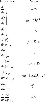
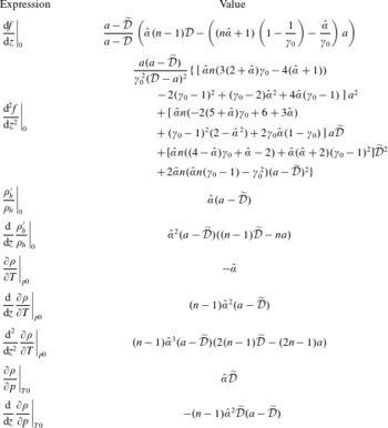
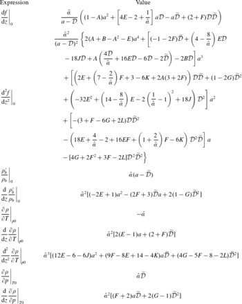
Some quantities related to the base flow, needed for the two-mode approximation, for the equation of state of an ideal gas.
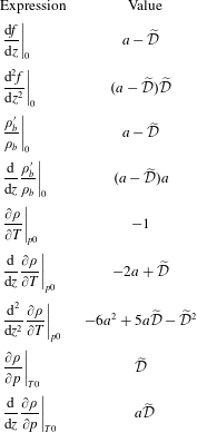
We also apply the analysis based on just two eigenmodes (
 $\cos (\unicode[STIX]{x03C0}z)$
and
 $\sin (2\unicode[STIX]{x03C0}z)$
), leading to (6.29) and (6.30), which are themselves issued from the critical relation (6.16). We need to derive some expressions from the equation of state: they are values of quantities at
 $z=0$
, relative to the base profile
 $f$
,
 $\unicode[STIX]{x1D70C}_{b}^{\prime }/\unicode[STIX]{x1D70C}_{b}$
,
 $(\unicode[STIX]{x2202}\unicode[STIX]{x1D70C}/\unicode[STIX]{x2202}T)|_{p}$
,
 $(\unicode[STIX]{x2202}\unicode[STIX]{x1D70C}/\unicode[STIX]{x2202}p)|_{T}$
and their derivatives at
 $z=0$
. They are listed in table 2 for the case of an ideal gas. The expressions for the base profile in table 2 are simple enough to be substituted in the two-mode general solutions (6.31) and (6.32). The
 $\sin (2\unicode[STIX]{x03C0}z)$
contributions
 $\unicode[STIX]{x1D716}$
,
 $\unicode[STIX]{x1D716}^{B}$
and
 $\unicode[STIX]{x1D716}^{ALA}$
to the exact model, quasi-Boussinesq and quasi-ALA approximations take the form
 $$\begin{eqnarray}\displaystyle & \displaystyle \unicode[STIX]{x1D716}=\frac{64}{117\unicode[STIX]{x03C0}^{2}}(a-\widetilde{{\mathcal{D}}}), & \displaystyle\end{eqnarray}$$
 $$\begin{eqnarray}\displaystyle & \displaystyle \unicode[STIX]{x1D716}^{B}=\frac{64}{117\unicode[STIX]{x03C0}^{2}}\left(a-\frac{7}{8}\widetilde{{\mathcal{D}}}\right), & \displaystyle\end{eqnarray}$$
 $$\begin{eqnarray}\displaystyle & \displaystyle \unicode[STIX]{x1D716}^{ALA}=\frac{64}{117\unicode[STIX]{x03C0}^{2}}\left(\frac{9}{8}a-\widetilde{{\mathcal{D}}}\right). & \displaystyle\end{eqnarray}$$
The corresponding critical superadiabatic Rayleigh number is obtained from (6.32) as an expansion of degree two in
 $a$
and
 ${\mathcal{D}}$
. We also obtain approximate critical Rayleigh numbers in the quasi-Boussinesq and quasi-ALA approximations. The differences between these critical Rayleigh numbers and the classical Boussinesq value
 $27\unicode[STIX]{x03C0}^{4}/4$
are denoted
 $\text{d}Ra_{SA}^{x}$
,
 $\text{d}Ra_{SA}^{B}$
and
 $\text{d}Ra_{SA}^{ALA}$
:
 $$\begin{eqnarray}\displaystyle \text{d}Ra_{SA}^{x} & = & \displaystyle \!\left[2\unicode[STIX]{x03C0}^{2}-\frac{320}{39}\right]\widetilde{{\mathcal{D}}}^{2}+\!\left[\frac{9\unicode[STIX]{x03C0}^{4}}{8}-\frac{17\unicode[STIX]{x03C0}^{2}}{4}+\frac{512}{13}\right]a\widetilde{{\mathcal{D}}}-\!\left[\frac{27\unicode[STIX]{x03C0}^{4}}{16}-\frac{63\unicode[STIX]{x03C0}^{2}}{8}+\frac{1216}{39}\right]a^{2},\nonumber\\ \displaystyle & \simeq & \displaystyle 11.53\widetilde{{\mathcal{D}}}^{2}+107.02a\widetilde{{\mathcal{D}}}-117.83a^{2},\end{eqnarray}$$
 $$\begin{eqnarray}\displaystyle \text{d}Ra_{SA}^{B} & = & \displaystyle -\frac{736}{39}\widetilde{{\mathcal{D}}}^{2}+\left[\frac{9\unicode[STIX]{x03C0}^{4}}{8}-\frac{9\unicode[STIX]{x03C0}^{2}}{2}+\frac{640}{13}\right]a\widetilde{{\mathcal{D}}}-\left[\frac{27\unicode[STIX]{x03C0}^{4}}{16}-\frac{63\unicode[STIX]{x03C0}^{2}}{8}+\frac{1216}{39}\right]a^{2},\nonumber\\ \displaystyle & \simeq & \displaystyle -18.87\widetilde{{\mathcal{D}}}^{2}+114.40a\widetilde{{\mathcal{D}}}-117.83a^{2},\end{eqnarray}$$
 $$\begin{eqnarray}\displaystyle \text{d}Ra_{SA}^{ALA} & = & \displaystyle \left[2\unicode[STIX]{x03C0}^{2}-\frac{320}{39}\right]\widetilde{{\mathcal{D}}}^{2}+\left[\frac{9\unicode[STIX]{x03C0}^{4}}{8}-\frac{25\unicode[STIX]{x03C0}^{2}}{4}+\frac{64}{3}\right]a\widetilde{{\mathcal{D}}}-\left[\frac{27\unicode[STIX]{x03C0}^{4}}{16}-\frac{61\unicode[STIX]{x03C0}^{2}}{8}+\frac{544}{39}\right]a^{2},\nonumber\\ \displaystyle & \simeq & \displaystyle 11.53\widetilde{{\mathcal{D}}}^{2}+69.23a\widetilde{{\mathcal{D}}}-103.07a^{2}.\end{eqnarray}$$
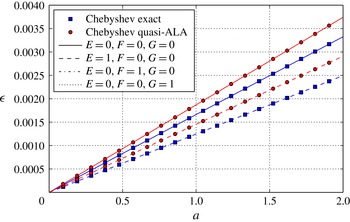
Asymmetrical contribution
 $\unicode[STIX]{x1D716}$
of the
 $\sin (2\unicode[STIX]{x03C0}z)$
mode to the critical eigenmode, for an ideal gas as a function of the temperature gradient
 $a$
of the base linear solution, for a negligible
 ${\mathcal{D}}=10^{-8}$
and a ratio of heat capacities
 $\unicode[STIX]{x1D6FE}$
equal to
 $5/3$
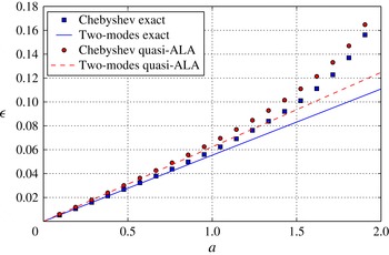
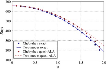
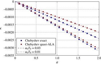
. The label ‘Chebyshev exact’ denotes the numerical solution of the exact model using a Chebyshev expansion (usually 17 polynomials), while the label ‘Chebyshev quasi-ALA’ corresponds to the solutions of the quasi-ALA model. The labels ‘Two-mode exact’ and ‘Two-mode quasi-ALA’ correspond to the approximate two-mode analytical solutions for the exact and quasi-ALA models. Note that when the dissipation number is negligible, the quasi-Boussinesq model and the exact model coincide.

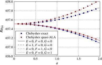
Linear stability critical threshold for the Rayleigh number for an ideal gas as a function of the temperature gradient
 $a$
of the base linear solution, for a negligible
 ${\mathcal{D}}=10^{-8}$
and a ratio of heat capacities
 $\unicode[STIX]{x1D6FE}$
equal to
 $5/3$
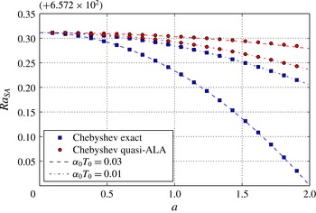
. Labels and line styles correspond to those of figure 2.

The eigenmode odd contribution
 $\unicode[STIX]{x1D716}$
obtained from the Chebyshev analysis is compared to that obtained from the two-mode analysis in figure 2 and for an ideal gas. As it is much easier experimentally to impose a large temperature gradient than large compressible effects, we first consider the case of a negligible dissipation number (
 ${\mathcal{D}}=10^{-8}$
). Exact and approximate eigenmode odd contributions are very similar throughout the whole range of
 $a$
(between
 $0$
and
 $2$
). Figure 3 shows how the critical Rayleigh number depends on the dimensionless temperature difference,
 $a$
, imposed between the bottom and the top. The Boussinesq value
 $27\unicode[STIX]{x03C0}^{4}/4$
is obtained in the limit
 $a=0$
(corresponding to a unity temperature ratio,
 $r=1$
). Increasing
 $a$
causes a decrease in the value of the superadiabatic critical Rayleigh number
 $Ra_{SA}^{x}$
. The approximate analysis (8.9) with two eigenmodes (
 $\cos (\unicode[STIX]{x03C0}z)$
and
 $\sin (2\unicode[STIX]{x03C0}z)$
) fits the numerical solution very well up to
 $a=1.5$
(corresponding to
 $r=7$
). With a negligible
 ${\mathcal{D}}$
, the quasi-Boussinesq approximation is identical to the exact analysis. The quasi-ALA approximation results are also plotted in figure 3, although this approximation is clearly not best at small
 ${\mathcal{D}}$
. Again, the quadratic two-mode approximation is very good for small values of
 $a$
. The results in figure 3 are independent of the ratio of heat capacities
 $\unicode[STIX]{x1D6FE}$
, as can be seen also on the two-mode approximations (8.9), (8.10) and (8.11).
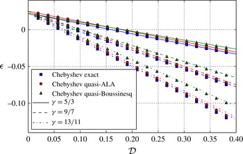
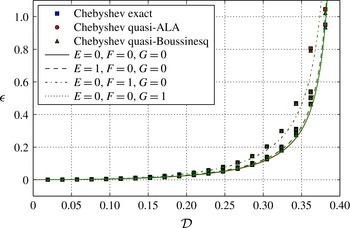
Asymmetrical contribution
 $\unicode[STIX]{x1D716}$
of the
 $\sin (2\unicode[STIX]{x03C0}z)$
mode to the critical eigenmode, for an ideal gas as a function of the dissipation number
 ${\mathcal{D}}$
, for a fixed temperature gradient
 $a=0.4$
(corresponding to a temperature ratio
 $r=1.5$
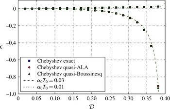
). The labels Chebyshev exact, quasi-ALA and quasi-Boussinesq correspond to numerical solutions obtained using the Chebyshev collocation eigenvalue calculations described in § 5, for the exact equations, quasi-ALA and Boussinesq models, respectively. The lines are the approximate two-mode analytical solutions described in § 6. Solid, dashed and dash-dotted lines correspond to three different values of the heat capacity ratio
 $\unicode[STIX]{x1D6FE}=5/3$
,
 $9/7$
and
 $13/11$
, respectively.

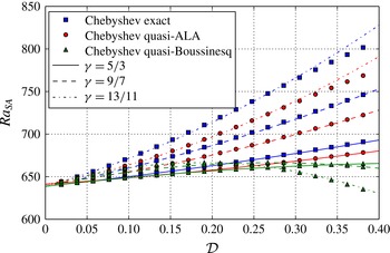
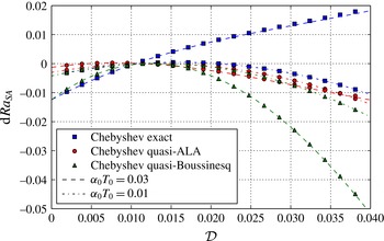
Linear stability critical threshold for the Rayleigh number for an ideal gas as a function of the dissipation number
 ${\mathcal{D}}$
, for a fixed temperature gradient
 $a=0.4$
(corresponding to a temperature ratio
 $r=1.5$
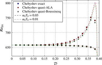
). The labels and line styles correspond to those of figure 4.

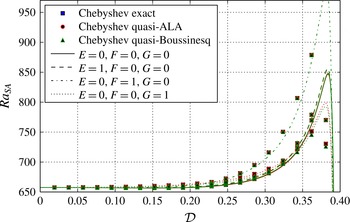
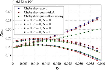
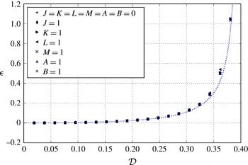
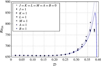
Figures 4 and 5 show how the asymmetrical contribution
 $\unicode[STIX]{x1D716}$
and the critical Rayleigh number depend on the dissipation number
 ${\mathcal{D}}$
for a fixed value of
 $a=0.4$
. The maximum value for
 ${\mathcal{D}}$
is
 $0.4$
so that superadiabaticity is ensured: for an ideal gas equation of state, this happens exactly when
 ${\mathcal{D}}<a$
, since the adiabatic gradient is uniform
 $\text{d}T_{a}/\text{d}z=-{\mathcal{D}}$
. At small
 ${\mathcal{D}}$
, the critical Rayleigh numbers increase with
 ${\mathcal{D}}$
and that tendency is enhanced as
 $\unicode[STIX]{x1D6FE}$
becomes closer to unity. We can see in figure 5 that the two-mode results (8.9), (8.10) and (8.11) are in excellent agreement with the Chebyshev calculations.
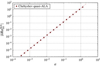
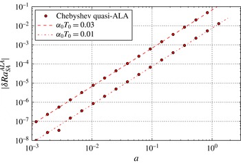
Absolute difference between the quasi-ALA critical Rayleigh number and the exact critical Rayleigh number, for an ideal gas as a function of
 $a$
, for
 ${\mathcal{D}}=10^{-8}$
and three values of the ratio of heat capacities,
 $\unicode[STIX]{x1D6FE}=5/3$
,
 $9/7$
and
 $13/11$
. The results using these three values are indistinguishable as expected from the approximate solutions (8.12) and (8.13).

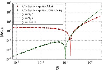
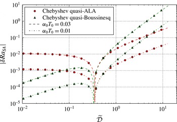
Absolute difference between the Boussinesq approximation critical Rayleigh number and the exact critical Rayleigh number, and absolute difference between the quasi-ALA and exact Rayleigh numbers, for an ideal gas as a function of
 $\widetilde{{\mathcal{D}}}$
, for
 $a=0.4$
and three values of the ratio of heat capacities,
 $\unicode[STIX]{x1D6FE}=5/3$
,
 $9/7$
and
 $13/11$
.

We shall now consider the results from a different point of view. Instead of looking at the Rayleigh number dependence, we shall plot the differences between the critical Rayleigh numbers of the quasi-Boussinesq and exact models and between the quasi-ALA and exact models:
 $\unicode[STIX]{x1D6FF}Ra_{SA}^{B}=Ra_{SA}^{B}-Ra_{SA}^{x}$
and
 $\unicode[STIX]{x1D6FF}Ra_{SA}^{ALA}=Ra_{SA}^{ALA}-Ra_{SA}^{x}$
. From (8.9), (8.10) and (8.11), we can extract the two-mode approximations for these differences:
 $$\begin{eqnarray}\displaystyle & \displaystyle \unicode[STIX]{x1D6FF}Ra_{SA}^{B}=-\frac{6\unicode[STIX]{x03C0}^{2}+32}{3}\widetilde{{\mathcal{D}}}^{2}-\frac{13\unicode[STIX]{x03C0}^{2}-512}{52}a\widetilde{{\mathcal{D}}}\simeq -30.41\widetilde{{\mathcal{D}}}^{2}+7.38a\widetilde{{\mathcal{D}}}, & \displaystyle\end{eqnarray}$$
 $$\begin{eqnarray}\displaystyle & \displaystyle \unicode[STIX]{x1D6FF}Ra_{SA}^{ALA}=-\frac{78\unicode[STIX]{x03C0}^{2}+704}{39}a\widetilde{{\mathcal{D}}}-\frac{13\unicode[STIX]{x03C0}^{2}-896}{52}a^{2}\simeq -37.79a\widetilde{{\mathcal{D}}}+14.76a^{2}. & \displaystyle\end{eqnarray}$$
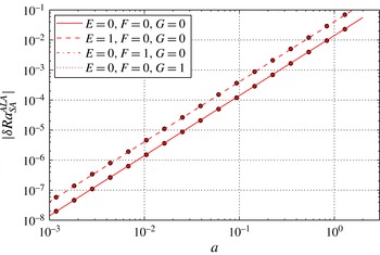
Plotting these differences provides an assessment of the quasi-Boussinesq and quasi-ALA models. Moreover, as we are interested in evaluating small departures from the exact model, we plot the absolute value of these differences in logarithmic coordinates. Figure 6 shows the difference between the quasi-ALA approximation and the exact models, for
 ${\mathcal{D}}=10^{-8}$
, as a function of
 $a$
. This difference is quadratic in
 $a$
, in agreement with (8.13).
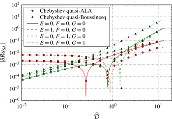
In figure 7, we plot the differences between the quasi-ALA and exact models and between the quasi-Boussinesq and exact models, for a constant value of
 $a=0.4$
, as a function of
 $\widetilde{{\mathcal{D}}}$
. Plotting these differences in terms of
 $\widetilde{{\mathcal{D}}}$
instead of
 ${\mathcal{D}}$
removes the dependence on
 $\unicode[STIX]{x1D6FE}$
that was observed in figure 5. All points collapse onto a single curve (for each model, quasi-Boussinesq and quasi-ALA) and the two-mode approximations (8.12) and (8.13) are in very good agreement with those obtained through the collocation Chebyshev eigenvalue solutions. These differences are quadratic in
 $a$
and
 $\widetilde{{\mathcal{D}}}$
, hence our plot for a constant
 $a$
and varying
 $\widetilde{{\mathcal{D}}}$
can exhibit constant values (
 $a^{2}$
contribution), linear regimes (
 $a\widetilde{{\mathcal{D}}}$
contribution) or quadratic regimes (
 $\widetilde{{\mathcal{D}}}^{2}$
contributions). Indeed, the quasi-Boussinesq model differs first linearly from the exact model at small
 $\widetilde{{\mathcal{D}}}$
, then quadratically when
 $\widetilde{{\mathcal{D}}}$
exceeds
 $a=0.4$
. The quasi-ALA model is different from the exact model at
 $\widetilde{{\mathcal{D}}}=0$
, so that
 $\unicode[STIX]{x1D6FF}Ra_{SA}^{ALA}$
is first constant as a function of
 $\widetilde{{\mathcal{D}}}$
, and is then a linear function of
 $\widetilde{{\mathcal{D}}}$
because it has no quadratic contribution (see (8.13)). A cusp between different regimes indicates simply a change of sign, as we plot the absolute value of the differences: use (8.12) and (8.13) to determine the sign. Figure 7 shows that the quasi-Boussinesq model is better at small
 $\widetilde{{\mathcal{D}}}$
and the quasi-ALA model is better at larger values. For a given value of the dissipation parameter
 ${\mathcal{D}}$
, decreasing the heat capacity ratio
 $\unicode[STIX]{x1D6FE}$
towards unity has the effect of increasing
 $\widetilde{{\mathcal{D}}}$
, so that the quasi-ALA model may be better than the quasi-Boussinesq model even for a relatively small dissipation parameter, provided
 $\unicode[STIX]{x1D6FE}$
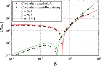
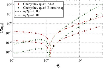
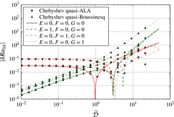
is close enough to unity. Figure 8 corresponds to a larger temperature ratio of
 $r=7$
(
 $a=1.5$
), for which the quadratic two-mode approximation is less good, although still acceptable.
Similar to figure 7, but with a temperature ratio
 $r=7$
(
 $a=1.5$
) instead of
 $r=1.5$
(
 $a=0.4$
).

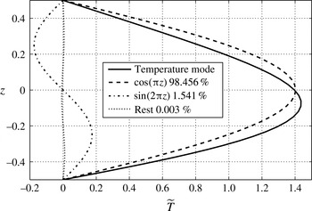
Temperature eigenmode, at the critical threshold for an ideal gas of
 $\unicode[STIX]{x1D6FE}=5/3$
,
 $a=1.5$
(equivalently
 $r=7$
),
 ${\mathcal{D}}=1.3$
. Its
 $\cos (\unicode[STIX]{x03C0}z)$
and
 $\sin (2\unicode[STIX]{x03C0}z)$
parts represent 98.456 % and 1.541 % of its
 $L^{2}$
norm. The rest (0.003 %) can hardly be distinguished from zero.

Figure 9 shows an eigenmode, for temperature, corresponding to the critical threshold, obtained for a temperature ratio equal to
 $7$
and a dissipation number equal to
 $1.3$
. The value of the ratio of heat capacities is
 $\unicode[STIX]{x1D6FE}=5/3$
. The eigenmode is projected on
 $\cos (\unicode[STIX]{x03C0}z)$
and
 $\sin (2\unicode[STIX]{x03C0}z)$
using the standard
 $L^{2}$
inner product on the interval
 $-0.5<z<0.5$
. The
 $L^{2}$
norm contributions of the
 $\cos (\unicode[STIX]{x03C0}z)$
and
 $\sin (2\unicode[STIX]{x03C0}z)$
modes are 98.456 % and 1.541 %, respectively, while the rest is 0.003 % only. This example is chosen so that the
 $\sin (2\unicode[STIX]{x03C0}z)$
contribution can be seen easily, i.e. with large values of the temperature gradient
 $a=1.5$
(corresponding to a temperature ratio of
 $r=7$
) and
 ${\mathcal{D}}=1.3$
. For small values of
 $a$
and
 ${\mathcal{D}}$
, suitable for our expansion near
 $a=0$
and
 ${\mathcal{D}}=0$
, the modes are closer to a pure
 $\cos (\unicode[STIX]{x03C0}z)$
function and the
 $\sin (2\unicode[STIX]{x03C0}z)$
function captures even better the difference between the mode and its cosine part. The example in figure 9 shows that the two functions
 $\cos (\unicode[STIX]{x03C0}z)$
and
 $\sin (2\unicode[STIX]{x03C0}z)$
are a good choice for an approximate representation of the eigenmodes.
8.2 Murnaghan’s equation of state
Let us now consider an equation of state suitable for condensed matter, liquid or solid, proposed by Murnaghan (Reference Murnaghan1951) with a temperature dependence appropriate for models of solid-state planetary interiors (Ricard Reference Ricard2007). This equation of state can be written as
 $$\begin{eqnarray}\left(\frac{\unicode[STIX]{x1D70C}}{\unicode[STIX]{x1D70C}_{0}}\right)^{n}=1+\frac{np}{K_{0}}-n\unicode[STIX]{x1D6FC}_{0}(T-T_{0}),\end{eqnarray}$$
with
 $n=3$
or
 $n=4$
for most solid materials, and
 $K_{0}$
and
 $\unicode[STIX]{x1D6FC}_{0}$
are constants. The reference density
 $\unicode[STIX]{x1D70C}_{0}$
is obtained for the reference temperature
 $T_{0}$
and pressure
 $p=0$
(the reference pressure is irrelevant as only pressure gradients play a role in the dynamical equations). This equation reproduces the observations that, for liquids and solids, the isothermal incompressibility
 $K_{T}=\unicode[STIX]{x1D70C}(\unicode[STIX]{x2202}p/\unicode[STIX]{x2202}\unicode[STIX]{x1D70C})|_{T}$
increases with compression,
 $$\begin{eqnarray}K_{T}=K_{0}\left(\frac{\unicode[STIX]{x1D70C}}{\unicode[STIX]{x1D70C}_{0}}\right)^{n},\end{eqnarray}$$
and that the coefficient of thermal expansion diminishes with compression,
 $$\begin{eqnarray}\unicode[STIX]{x1D6FC}=\unicode[STIX]{x1D6FC}_{0}\left(\frac{\unicode[STIX]{x1D70C}_{0}}{\unicode[STIX]{x1D70C}}\right)^{n}.\end{eqnarray}$$
We also need to derive the heat capacity from the equation of state. The thermodynamic relation
 $(\unicode[STIX]{x2202}c_{v}/\unicode[STIX]{x2202}\unicode[STIX]{x1D708})|_{T}=T(\unicode[STIX]{x2202}^{2}p/\unicode[STIX]{x2202}T^{2})|_{\unicode[STIX]{x1D708}}$
(where
 $\unicode[STIX]{x1D708}$
is the specific volume
 $1/\unicode[STIX]{x1D70C}$
) indicates that, for a solid following (8.14),
 $c_{v}$
is not a function of
 $\unicode[STIX]{x1D70C}$
, as the pressure is linear in
 $T$
for a given density. So
 $c_{v}$
can only be a function of temperature
 $T$
: any choice is valid in principle. We make the choice of a constant
 $c_{v0}$
, which is in agreement with the Dulong and Petit rule for condensed matter. It follows then from Mayer’s relation (6.9) that
 $$\begin{eqnarray}c_{p}=c_{v0}+\frac{\unicode[STIX]{x1D6FC}_{0}^{2}K_{0}T}{\unicode[STIX]{x1D70C}}\left(\frac{\unicode[STIX]{x1D70C}_{0}}{\unicode[STIX]{x1D70C}}\right)^{n}.\end{eqnarray}$$
With notation (6.10), using our dimensional scales, Murnaghan’s equation of state therefore takes the following dimensionless form:
 $$\begin{eqnarray}\unicode[STIX]{x1D70C}^{n}=1+\hat{\unicode[STIX]{x1D6FC}}\widetilde{{\mathcal{D}}}np-n\hat{\unicode[STIX]{x1D6FC}}(T-1).\end{eqnarray}$$
The base profile is determined as follows. The temperature base profile is independent of the equation of state, hence (4.3) is still valid. The derivative of (8.18) and the hydrostatic equation
 $\text{d}p_{b}/\text{d}z=-\unicode[STIX]{x1D70C}_{b}$
lead to a differential equation for the base density profile
 $\unicode[STIX]{x1D70C}_{b}$
:
 $$\begin{eqnarray}\frac{\text{d}\unicode[STIX]{x1D70C}_{b}}{\text{d}z}=-\hat{\unicode[STIX]{x1D6FC}}\widetilde{{\mathcal{D}}}\unicode[STIX]{x1D70C}_{b}^{2-n}+\hat{\unicode[STIX]{x1D6FC}}a\unicode[STIX]{x1D70C}_{b}^{1-n}.\end{eqnarray}$$
This equation is integrated numerically, under the condition that
 $\unicode[STIX]{x1D70C}_{b}=1$
at
 $z=0$
in accordance with our choice for the dimensional reference density
 $\unicode[STIX]{x1D70C}_{0}$
. The base pressure profile
 $p_{b}$
is then obtained from the equation of state (8.18).
In the resolution of the eigenvalue problem (5.5), (5.6), (5.7) and (5.8), we also need to determine the base profile for the dimensionless specific heat capacity
 $c_{pb}$
and expansivity
 $\unicode[STIX]{x1D6FC}_{b}$
. After non-dimensionalization, (8.16) can be written as
 $$\begin{eqnarray}\unicode[STIX]{x1D6FC}_{b}=\unicode[STIX]{x1D70C}_{b}^{-n},\end{eqnarray}$$
and (8.17) as
 $$\begin{eqnarray}c_{pb}=\frac{1}{\unicode[STIX]{x1D6FE}_{0}}+\frac{\unicode[STIX]{x1D6FE}_{0}-1}{\unicode[STIX]{x1D6FE}_{0}}T_{b}\unicode[STIX]{x1D70C}_{b}^{-1-n}.\end{eqnarray}$$
Coefficients of Taylor expansion of some quantities related to the base flow, for Murnaghan’s equation of state, for arbitrary values of
 $\unicode[STIX]{x1D6FE}_{0}=c_{p0}/c_{v0}$
and
 $\hat{\unicode[STIX]{x1D6FC}}=\unicode[STIX]{x1D6FC}_{0}T_{0}$
.

Asymmetrical contribution of the
 $\sin (2\unicode[STIX]{x03C0}z)$
mode to the critical eigenmode, for a Murnaghan equation of state as a function of the temperature gradient
 $a$
of the base linear solution, for a negligible
 ${\mathcal{D}}=10^{-8}$
. The label ‘Chebyshev exact’ denotes the numerical solution of the exact model using a Chebyshev expansion (usually 17 polynomials), while the label ‘Chebyshev quasi-ALA’ corresponds to the solutions of the quasi-ALA model. The dashed and dash-dotted lines correspond to the approximate two-mode analytical solutions for the exact and quasi-ALA models, at
 $\hat{\unicode[STIX]{x1D6FC}}=\unicode[STIX]{x1D6FC}_{0}T_{0}=0.03$
and
 $0.01$
, respectively. The ratio of heat capacities and integer
 $n$
in the equation of state (8.18) are kept constant,
 $\unicode[STIX]{x1D6FE}_{0}=1.03$
and
 $n=3$
. Note that, when the dissipation number is negligible, the quasi-Boussinesq model and the exact model coincide.

Linear stability critical threshold for the Rayleigh number for a Murnaghan equation of state as a function of the temperature gradient
 $a$
of the base linear solution, for a negligible
 ${\mathcal{D}}=10^{-8}$
. The labels are similar to those of figure 10.

Asymmetrical contribution of the
 $\sin (2\unicode[STIX]{x03C0}z)$
mode to the critical eigenmode, for the Rayleigh number for a Murnaghan equation of state as a function of the dissipation number
 ${\mathcal{D}}$
, for a fixed temperature gradient
 $a=0.4$
(corresponding to a temperature ratio
 $r=1.5$
). The labels Chebyshev exact, quasi-ALA and quasi-Boussinesq correspond to numerical solutions obtained using the Chebyshev collocation eigenvalue calculations described in § 5, for the exact equations, quasi-ALA and Boussinesq approximations, respectively. The lines are the analytical two-mode solutions described in § 6. Dashed and dash-dotted lines correspond to two different values for the product of the expansion coefficient and temperature at
 $z=0$
,
 $\hat{\unicode[STIX]{x1D6FC}}=\unicode[STIX]{x1D6FC}_{0}T_{0}=0.03$
and
 $0.01$
, while the heat capacity ratio at
 $z=0$
is kept constant
 $\unicode[STIX]{x1D6FE}_{0}=1.03$
and
 $n=3$
.

Linear stability critical threshold for the Rayleigh number for a Murnaghan equation of state as a function of the dissipation number
 ${\mathcal{D}}$
, for a fixed temperature gradient
 $a=0.4$
(corresponding to a temperature ratio
 $r=1.5$
). The labels are defined in figure 12.

Same as figure 13 with a close-up around small values of
 ${\mathcal{D}}$
, between
 $0$
and
 $0.04$
. The difference
 $\text{d}Ra_{SA}=Ra_{SA}-27\unicode[STIX]{x03C0}^{4}/4$
is plotted instead of
 $Ra_{SA}$
.

In table 3, we show the expression of all quantities needed for the approximate two-mode analysis: the derivatives of the function
 $f(z)$
at
 $z=0$
, and other quantities, can then be determined using (8.20) and (8.21) up to degree two in
 $a$
and
 ${\mathcal{D}}$
. From these expressions, using (6.29) and (6.30), we obtain the approximate expressions for the critical Rayleigh numbers with and without the effect of compressibility for the small disturbances.
With table 3 and the general solutions (6.31) and (6.32), we have the quadratic departure of the superadiabatic critical Rayleigh number in terms of the parameters
 $a$
and
 ${\mathcal{D}}$
. It would actually take too much space to display
 $\text{d}Ra_{SA}$
once the quantities in table 3 are substituted in those general equations. However, it is possible to do so for the
 $\sin (2\unicode[STIX]{x03C0}z)$
contributions. The coefficients
 $\unicode[STIX]{x1D716}$
(coefficient of
 $\sin (2\unicode[STIX]{x03C0}z)$
) obtained by the two-mode analysis (6.31), (7.5) and (7.6) are the following, for the exact model, quasi-Boussinesq and quasi-ALA approximations:
 $$\begin{eqnarray}\displaystyle & \displaystyle \unicode[STIX]{x1D716}^{x}=\frac{8\hat{\unicode[STIX]{x1D6FC}}[a-\widetilde{{\mathcal{D}}}]}{117\unicode[STIX]{x03C0}^{2}}\left[9\frac{(n-1){\mathcal{D}}-[(1-\unicode[STIX]{x1D6FE}_{0}^{-1})(n+\hat{\unicode[STIX]{x1D6FC}}^{-1})-\unicode[STIX]{x1D6FE}_{0}^{-1}]a}{a-{\mathcal{D}}}-n-2\right]-\frac{8\hat{\unicode[STIX]{x1D6FC}}\widetilde{{\mathcal{D}}}}{117\unicode[STIX]{x03C0}^{2}},\qquad & \displaystyle\end{eqnarray}$$
 $$\begin{eqnarray}\displaystyle & \displaystyle \unicode[STIX]{x1D716}^{B}=\frac{8\hat{\unicode[STIX]{x1D6FC}}[a-\widetilde{{\mathcal{D}}}]}{117\unicode[STIX]{x03C0}^{2}}\left[9\frac{(n-1){\mathcal{D}}-[(1-\unicode[STIX]{x1D6FE}_{0}^{-1})(n+\hat{\unicode[STIX]{x1D6FC}}^{-1})-\unicode[STIX]{x1D6FE}_{0}^{-1}]a}{a-{\mathcal{D}}}-n-2\right], & \displaystyle\end{eqnarray}$$
 $$\begin{eqnarray}\displaystyle & \displaystyle \unicode[STIX]{x1D716}^{ALA}=\frac{8\hat{\unicode[STIX]{x1D6FC}}[a-\widetilde{{\mathcal{D}}}]}{117\unicode[STIX]{x03C0}^{2}}\left[9\frac{(n-1){\mathcal{D}}-[(1-\unicode[STIX]{x1D6FE}_{0}^{-1})(n+\hat{\unicode[STIX]{x1D6FC}}^{-1})-\unicode[STIX]{x1D6FE}_{0}^{-1}]a}{a-{\mathcal{D}}}-n-1\right]. & \displaystyle\end{eqnarray}$$
Similarly, the differences between critical superadiabatic Rayleigh numbers obtained from the quasi-Boussinesq or quasi-ALA approximations and the exact model (7.7) and (7.8) are also short enough to be shown explicitly:
 $$\begin{eqnarray}\displaystyle & \displaystyle \unicode[STIX]{x1D6FF}Ra_{SA}^{B}=\left[\frac{9n-1}{4}\unicode[STIX]{x03C0}^{2}-\frac{256n-128}{39}\right]\hat{\unicode[STIX]{x1D6FC}}^{2}a\widetilde{{\mathcal{D}}}-\left[\frac{9n-1}{4}\unicode[STIX]{x03C0}^{2}-\frac{256n-416}{39}\right]\hat{\unicode[STIX]{x1D6FC}}^{2}\widetilde{{\mathcal{D}}}^{2},\qquad & \displaystyle\end{eqnarray}$$
 $$\begin{eqnarray}\displaystyle & \displaystyle \unicode[STIX]{x1D6FF}Ra_{SA}^{ALA}=\left[\frac{9n+8}{4}\unicode[STIX]{x03C0}^{2}-\frac{256n-416}{39}\right]\hat{\unicode[STIX]{x1D6FC}}^{2}a^{2}-\left[\frac{9n+8}{4}\unicode[STIX]{x03C0}^{2}-\frac{256n-704}{39}\right]\hat{\unicode[STIX]{x1D6FC}}^{2}a\widetilde{{\mathcal{D}}}.\qquad & \displaystyle\end{eqnarray}$$
Figure 11 shows the dependence of the critical Rayleigh numbers for the exact model and quasi-ALA approximation on the base temperature gradient
 $a$
for a negligible dissipation parameter
 ${\mathcal{D}}=10^{-8}$
and a constant
 $\unicode[STIX]{x1D6FE}_{0}=1.03$
and
 $n=3$
. These critical Rayleigh numbers are also obtained with the two-mode analysis with an excellent accuracy. Two different values of
 $\hat{\unicode[STIX]{x1D6FC}}$
are considered and we can see that the departure of the critical Rayleigh numbers from
 $27\unicode[STIX]{x03C0}^{4}/4$
gets smaller as
 $\hat{\unicode[STIX]{x1D6FC}}$
diminishes. Figure 12 shows the dependence of the asymmetrical contribution of the
 $\sin (2\unicode[STIX]{x03C0}z)$
mode to the critical eigenmode on
 ${\mathcal{D}}$
for a fixed value of the base temperature gradient
 $a=0.4$
. The ratio of heat capacities is kept constant at
 $\unicode[STIX]{x1D6FE}_{0}=1.03$
and two values of
 $\hat{\unicode[STIX]{x1D6FC}}=\unicode[STIX]{x1D6FC}_{0}T_{0}=0.03$
and
 $0.01$
are considered. The two-mode analysis provides a good fit throughout the whole range of
 ${\mathcal{D}}$
. Correspondingly, figure 13 shows the dependence of the critical Rayleigh numbers (exact, quasi-Boussinesq and quasi-ALA) on
 ${\mathcal{D}}$
for the same conditions, with an equally good fit of the two-mode analysis to the numerical data obtained using the Chebyshev expansion.
A close-up around small values of
 ${\mathcal{D}}$
is shown in figure 14, emphasizing the quality of the approximate analysis and its ability to recover small variations of the critical Rayleigh numbers.
Absolute difference between the critical Rayleigh number of the quasi-ALA and exact model, with Murnaghan’s equation of state and for a negligible dissipation number equal to
 ${\mathcal{D}}=10^{-8}$
. The difference is plotted as a function of
 $a$
, for two values of
 $\unicode[STIX]{x1D6FC}_{0}T_{0}=\hat{\unicode[STIX]{x1D6FC}}$
(
 $0.03$
and
 $0.01$
) and
 $\unicode[STIX]{x1D6FE}_{0}=1.03$
. The parameter
 $n$
in Murnaghan’s equation of state is equal to
 $3$
in all cases.

Similar to figure 13 but in logarithmic coordinates and for the absolute difference of the critical Rayleigh numbers between the approximations and exact model, for two values of
 $\unicode[STIX]{x1D6FC}_{0}T_{0}=\hat{\unicode[STIX]{x1D6FC}}$
(
 $0.03$
and
 $0.01$
) and
 $\unicode[STIX]{x1D6FE}_{0}=1.03$
.

Similar to figure 16 but the temperature ratio is
 $r=7$
(
 $a=1.5$
) instead of
 $r=1.5$
(
 $a=0.4$
).

In figure 15, we plot the absolute difference of the quasi-ALA and exact critical Rayleigh numbers, for a negligible dissipation parameter and varying temperature gradients, which can be seen to be very well approximated by the two-mode analysis. This is also the case, for a constant temperature gradient
 $a=0.4$
and varying dissipation parameter, shown in figure 16. With a larger temperature gradient
 $a=1.5$
, and for the largest value of the dissipation parameter, we can detect a small deviation from the two-mode analysis (see figure 17). These results, shown in figures 16 and 17, confirm that the quasi-ALA approximation is much better than the quasi-Boussinesq approximation when
 $\widetilde{{\mathcal{D}}}$
is larger than
 $a$
. Obviously, that condition is most easily fulfilled when
 $\unicode[STIX]{x1D6FE}_{0}$
is very close to
 $1$
.
8.3 A generic equation of state
An examination of the previous results – for instance (8.25) or (8.26) – reveals that the first derivatives of density with respect to temperature or pressure (related to
 $\hat{\unicode[STIX]{x1D6FC}}$
and
 ${\mathcal{D}}$
, respectively) are not the only parameters affecting the critical Rayleigh numbers: the parameter
 $n$
is not related to the first derivatives and yet affects the critical Rayleigh numbers. The predictions of our two-mode semi-analytic model are based on a set of quantities (those listed in tables 2 and 3, for the ideal gas and the Murnaghan fluid). These quantities involve up to the third degree of the equation of state in the terms
 $\text{d}^{2}((\unicode[STIX]{x2202}\unicode[STIX]{x1D70C}/\unicode[STIX]{x2202}T)|_{p0})/\text{d}z^{2}$
and
 $(\text{d}^{2}f/\text{d}z^{2})|_{0}$
, because any differentiation along
 $z$
is a combination of derivatives with respect to temperature and pressure, and because
 $c_{p}$
(in
 $f$
) is itself already based on a derivative of the equation of state. A generic equation of state that would completely determine the Rayleigh number with a second-order precision should extend to degree three in
 $p$
and
 $T$
.
In fact, it turns out that it is mathematically more convenient to expand the specific volume
 $\unicode[STIX]{x1D708}=1/\unicode[STIX]{x1D70C}$
with respect to temperature and pressure, rather than density. So a dimensionless equation of state can be written:
 $$\begin{eqnarray}\displaystyle \unicode[STIX]{x1D708} & = & \displaystyle \frac{1}{\unicode[STIX]{x1D70C}}=1+\hat{\unicode[STIX]{x1D6FC}}(T-1)-\hat{\unicode[STIX]{x1D6FC}}\widetilde{{\mathcal{D}}}p+\hat{\unicode[STIX]{x1D6FC}}^{2}E(T-1)^{2}+\hat{\unicode[STIX]{x1D6FC}}^{2}\widetilde{{\mathcal{D}}}Fp(T-1)+\hat{\unicode[STIX]{x1D6FC}}^{2}\widetilde{{\mathcal{D}}}^{2}Gp^{2}\nonumber\\ \displaystyle & & \displaystyle +\,\hat{\unicode[STIX]{x1D6FC}}^{3}J(T-1)^{3}+\hat{\unicode[STIX]{x1D6FC}}^{3}\widetilde{{\mathcal{D}}}Kp(T-1)^{2}+\hat{\unicode[STIX]{x1D6FC}}^{3}\widetilde{{\mathcal{D}}}^{2}Lp^{2}(T-1)+\hat{\unicode[STIX]{x1D6FC}}^{3}\widetilde{{\mathcal{D}}}^{3}Mp^{3}.\end{eqnarray}$$
The expression for the dimensionless derivative of
 $\unicode[STIX]{x1D708}$
with respect to
 $p$
is found to be
 $-\hat{\unicode[STIX]{x1D6FC}}\widetilde{{\mathcal{D}}}$
and the coefficients
 $E$
,
 $F$
,
 $G$
,
 $J$
,
 $K$
,
 $L$
and
 $M$
are dimensionless parameters proportional to the second and third derivatives of the specific volume. We have chosen to make these coefficients independent of gravity
 $g$
by multiplying systematically any occurrence of the dimensionless pressure
 $p$
by the dissipation parameter
 $\widetilde{{\mathcal{D}}}$
.
Coefficients of Taylor expansion of some quantities related to the base flow, for a generic equation of state (8.27).

We apply the same procedure for this generic equation of state as for the equations of state considered previously. In order to obtain an expression for
 $c_{p}$
, we integrate the relation
 $$\begin{eqnarray}\left.\frac{\unicode[STIX]{x2202}c_{p}}{\unicode[STIX]{x2202}p}\right|_{T}=\left.-\frac{{\mathcal{D}}}{\hat{\unicode[STIX]{x1D6FC}}}T\frac{\unicode[STIX]{x2202}^{2}\unicode[STIX]{x1D708}}{\unicode[STIX]{x2202}T^{2}}\right|_{p},\end{eqnarray}$$
which leads to
 $$\begin{eqnarray}c_{p}=1+\hat{\unicode[STIX]{x1D6FC}}A(T-1)+\hat{\unicode[STIX]{x1D6FC}}^{2}B(T-1)^{2}-\hat{\unicode[STIX]{x1D6FC}}{\mathcal{D}}T(2Ep+6\hat{\unicode[STIX]{x1D6FC}}Jp(T-1)+\hat{\unicode[STIX]{x1D6FC}}\widetilde{{\mathcal{D}}}Kp^{2}),\end{eqnarray}$$
where the
 $p$
-independent integration term has been expressed up to degree two by introducing two extra coefficients
 $A$
and
 $B$
.
The reference temperature is still
 $$\begin{eqnarray}T_{b}(z)=1-az,\end{eqnarray}$$
with a uniform gradient.
All quantities needed in the approximate analysis have been determined and listed in table 4. With table 4 and the general solutions obtained in §§ 6 and 7, the analytic expressions for
 $\unicode[STIX]{x1D716}$
and
 $\text{d}Ra_{SA}$
(and corresponding results for the quasi-Boussinesq and quasi-ALA approximations) are explicitly determined. Some results, like
 $\text{d}Ra_{SA}$
, would take a page to display when the substitution is made. Others are shorter. For instance, the relative amplitude of the
 $\sin (2\unicode[STIX]{x03C0}z)$
component relative to the
 $\cos (\unicode[STIX]{x03C0}z)$
component can be written entirely in terms of the elementary governing coefficients:
 $$\begin{eqnarray}\displaystyle \unicode[STIX]{x1D716}^{x}=\frac{8\hat{\unicode[STIX]{x1D6FC}}}{\unicode[STIX]{x03C0}^{2}}\left[\frac{(1-A)a^{2}-a\widetilde{{\mathcal{D}}}+\left[4E+\displaystyle \frac{1}{\hat{\unicode[STIX]{x1D6FC}}}-2\right]a{\mathcal{D}}+(F+2)\widetilde{{\mathcal{D}}}{\mathcal{D}}}{13(a-{\mathcal{D}})}-\frac{(1+2E)a+F\widetilde{{\mathcal{D}}}}{117}\right], & & \displaystyle \nonumber\\ \displaystyle & & \displaystyle\end{eqnarray}$$
 $$\begin{eqnarray}\displaystyle \unicode[STIX]{x1D716}^{B} & = & \displaystyle \frac{8\hat{\unicode[STIX]{x1D6FC}}}{\unicode[STIX]{x03C0}^{2}}\left[\frac{(1-A)a^{2}-a\widetilde{{\mathcal{D}}}+\left[4E+\displaystyle \frac{1}{\hat{\unicode[STIX]{x1D6FC}}}-2\right]a{\mathcal{D}}+(F+2)\widetilde{{\mathcal{D}}}{\mathcal{D}}}{13(a-{\mathcal{D}})}\right.\nonumber\\ \displaystyle & & \displaystyle -\,\left.\frac{(1+2E)a+(F-1)\widetilde{{\mathcal{D}}}}{117}\right],\end{eqnarray}$$
 $$\begin{eqnarray}\displaystyle \unicode[STIX]{x1D716}^{ALA}=\frac{8\hat{\unicode[STIX]{x1D6FC}}}{\unicode[STIX]{x03C0}^{2}}\left[\frac{(1-A)a^{2}-a\widetilde{{\mathcal{D}}}+\left[4E+\displaystyle \frac{1}{\hat{\unicode[STIX]{x1D6FC}}}-2\right]a{\mathcal{D}}+(F+2)\widetilde{{\mathcal{D}}}{\mathcal{D}}}{13(a-{\mathcal{D}})}-\frac{2Ea+F\widetilde{{\mathcal{D}}}}{117}\right].\qquad & & \displaystyle\end{eqnarray}$$
We can also expand the two-mode approximations (7.7) and (7.8), using table 4, for the difference between the quasi-Boussinesq approximation and the exact model
 $\unicode[STIX]{x1D6FF}Ra_{SA}^{B}$
, and between the quasi-ALA approximation and exact model
 $\unicode[STIX]{x1D6FF}Ra_{SA}^{ALA}$
:
 $$\begin{eqnarray}\displaystyle \unicode[STIX]{x1D6FF}Ra_{SA}^{B} & = & \displaystyle -\left[-{\textstyle \frac{5}{2}}\unicode[STIX]{x03C0}^{2}+{\textstyle \frac{224}{13}}+{\textstyle \frac{9}{2}}\unicode[STIX]{x03C0}^{2}G+{\textstyle \frac{256}{39}}F\right]\hat{\unicode[STIX]{x1D6FC}}^{2}\widetilde{{\mathcal{D}}}^{2}\nonumber\\ \displaystyle & & \displaystyle -\,\left[{\textstyle \frac{5}{2}}\unicode[STIX]{x03C0}^{2}-{\textstyle \frac{128}{13}}+{\textstyle \frac{9}{4}}\unicode[STIX]{x03C0}^{2}F+{\textstyle \frac{512}{39}}E\right]\hat{\unicode[STIX]{x1D6FC}}^{2}a\widetilde{{\mathcal{D}}},\end{eqnarray}$$
 $$\begin{eqnarray}\displaystyle \unicode[STIX]{x1D6FF}Ra_{SA}^{ALA} & = & \displaystyle \left[{\textstyle \frac{1}{4}}\unicode[STIX]{x03C0}^{2}-{\textstyle \frac{320}{13}}+\left({\textstyle \frac{9}{4}}\unicode[STIX]{x03C0}^{2}-{\textstyle \frac{256}{39}}\right)F\right]\hat{\unicode[STIX]{x1D6FC}}^{2}a\widetilde{{\mathcal{D}}}\nonumber\\ \displaystyle & & \displaystyle +\,\left[{\textstyle \frac{1}{4}}\unicode[STIX]{x03C0}^{2}+{\textstyle \frac{224}{13}}+\left({\textstyle \frac{9}{2}}\unicode[STIX]{x03C0}^{2}-{\textstyle \frac{512}{39}}\right)E\right]\hat{\unicode[STIX]{x1D6FC}}^{2}a^{2}.\end{eqnarray}$$
The two-mode analysis and table 4 indicate that the quadratic departure of the suparadiabatic threshold from the Boussinesq limit (6.32) depends on all coefficients of the cubic expansion of the generic equation of state (8.27) and on the extra free coefficients
 $A$
and
 $B$
in the expression for the heat capacity (8.29). Only
 $M$
(related to
 $\unicode[STIX]{x2202}^{3}\unicode[STIX]{x1D708}/\unicode[STIX]{x2202}p^{3}$
) has no influence, as expected, because that particular third derivative is not involved in the relevant coefficients
 $\text{d}^{2}((\unicode[STIX]{x2202}\unicode[STIX]{x1D70C}/\unicode[STIX]{x2202}T)|_{p0})/\text{d}z^{2}$
and
 $(\text{d}^{2}f/\text{d}z^{2})|_{0}$
. The two-mode analyses of the quasi-Boussinesq and quasi-ALA models show that the difference of the critical superadiabatic Rayleigh numbers depends entirely on the second-order expansion of the equation of state:
 $J$
,
 $K$
,
 $L$
and
 $M$
do not affect the differences (8.34) and (8.35), neither do
 $A$
and
 $B$
.
Asymmetrical contribution of the
 $\sin (2\unicode[STIX]{x03C0}z)$
mode to the critical eigenmode, for a generic equation of state (8.27) as a function of the temperature gradient
 $a$
of the base linear solution, for a negligible
 ${\mathcal{D}}=10^{-8}$
. The label ‘Chebyshev exact’ denotes the numerical solution of the exact model using a Chebyshev expansion (usually 17 polynomials), while the label ‘Chebyshev quasi-ALA’ corresponds to the solutions of the quasi-ALA model. The solid, dashed, dash-dotted and dotted lines correspond to the approximate two-mode analytical solutions for the exact and quasi-ALA models, for different choices of the dimensionless parameters
 $E$
,
 $F$
and
 $G$
, respectively. The ratio of heat capacities and the product of temperature and the thermal expansion coefficient are kept constant,
 $\unicode[STIX]{x1D6FE}_{0}=1.03$
and
 $\hat{\unicode[STIX]{x1D6FC}}=\unicode[STIX]{x1D6FC}_{0}T_{0}=0.03$
. When the dissipation number is negligible, the quasi-Boussinesq model and the exact model coincide.


With so many parameters (nine parameters without counting
 $\hat{\unicode[STIX]{x1D6FC}}$
,
 $a$
and
 $\widetilde{{\mathcal{D}}}$
), it is impossible to show and explore all the possible cases. Similarly to what we have computed for the ideal gas and the Murnaghan equations of state, we start by depicting a few cases where the compressible effects are small,
 ${\mathcal{D}}=10^{-8}$
, but the temperature difference large, which are conditions that could be easily reproduced experimentally. In figures 18 and 19, we plot the asymmetrical contributions of the critical eigenmode
 $\unicode[STIX]{x1D716}$
and the corresponding changes in the critical Rayleigh number when only the second-order coefficients of the generic equation of state (i.e.
 $E$
,
 $F$
and
 $G$
) are changed. In agreement with (8.31) or (8.33), when
 ${\mathcal{D}}\ll 1$
and
 $A$
is constant,
 $\unicode[STIX]{x1D716}$
is a function only of
 $E$
, which corresponds very precisely to the numerical estimates (see figure 18). The Rayleigh numbers of the exact and ALA cases are also functions only of
 $E$
(see figure 18).
Asymmetrical contribution of the
 $\sin (2\unicode[STIX]{x03C0}z)$
mode to the critical eigenmode, for the Rayleigh number for a generic equation of state (8.27) as a function of the dissipation number
 ${\mathcal{D}}$
, for a fixed temperature gradient
 $a=0.4$
(corresponding to a temperature ratio
 $r=1.5$
). The labels Chebyshev exact, quasi-ALA and quasi-Boussinesq correspond to numerical solutions obtained using the Chebyshev collocation eigenvalue calculations described in § 5, for the exact equations, quasi-ALA and Boussinesq approximations, respectively. The lines are the analytical two-mode solutions described in § 6. Solid, dashed, dash-dotted and dotted lines correspond to different selections of the parameters
 $E$
,
 $F$
and
 $G$
, while the heat capacity ratio and
 $\unicode[STIX]{x1D6FC}T$
at
 $z=0$
are kept constant,
 $\unicode[STIX]{x1D6FE}_{0}=1.03$
and
 $\hat{\unicode[STIX]{x1D6FC}}=\unicode[STIX]{x1D6FC}_{0}T_{0}=0.03$
, and the other parameters of the generic equation of state are set to zero:
 $J=K=L=M=A=B=0$
.

Linear stability critical threshold for the Rayleigh number for a generic equation of state (8.27) as a function of the dissipation number
 ${\mathcal{D}}$
, for a fixed temperature gradient
 $a=0.4$
(corresponding to a temperature ratio
 $r=1.5$
). The labels are similar to those in figure 20.

Same as figure 21 with a close-up around small values of
 ${\mathcal{D}}$
, between
 $0$
and
 $0.04$
.

We then compute a few cases with a fixed temperature interval
 $a=0.4$
but for varying compressible effects. Like for the cases illustrated in the two previous figures, we only vary the second-order coefficients of the equation of state. The asymmetrical contributions of the critical eigenmode
 $\unicode[STIX]{x1D716}$
and the corresponding change in the critical
 $Ra$
number are depicted in figures 20 and 21. In these two figures, an asymptote is present at
 ${\mathcal{D}}=0.4$
because of the singular term in
 $a-{\mathcal{D}}$
in the various analytical expressions. Here, again, the two-mode expansion captures reasonably accurately the numerical results. However, the two-mode expansion is even better for small values of
 ${\mathcal{D}}$
since it is a Taylor expansion of degree two. In figure 22, we show a close-up of figure 21 at small
 ${\mathcal{D}}$
(between
 $0$
and
 $0.04$
) and it is apparent that each coefficient
 $E$
,
 $F$
and
 $G$
has a specific influence on the critical Rayleigh number, which is very accurately modelled by the two-mode analysis.
Same as figure 20, but only the results from the exact governing equations are shown, along with its two-mode approximation. Now the parameters
 $E$
,
 $F$
and
 $G$
of the equation of state (8.27) are set to zero, while each of the other parameters (
 $J$
,
 $K$
,
 $L$
,
 $M$
,
 $A$
and
 $B$
) is set to
 $1$
in turn.

Same as figure 21, but only the results from the exact governing equations are shown, along with its two-mode approximation. Now the parameters
 $E$
,
 $F$
and
 $G$
of the equation of state (8.27) are set to zero, while each of the other parameters (
 $J$
,
 $K$
,
 $L$
,
 $M$
,
 $A$
and
 $B$
) is set to
 $1$
in turn.

Same as figure 24 with a close-up around small values of
 ${\mathcal{D}}$
, between
 $0$
and
 $0.04$
. It is clear that all parameters have an impact on the critical Rayleigh number, except
 $M$
(
 $+$
and
 $\times$
symbols superimpose), as predicted by the approximate analysis.

We now test the effects of the third-order terms (i.e.
 $J$
,
 $K$
,
 $L$
and
 $M$
, see (8.27)) as well as of the two terms controlling the heat capacity at reference pressure (
 $A$
and
 $B$
, see (8.29)) in figures 23–25. In all these simulations the temperature gradient is fixed to
 $a=0.4$
. We only compare the solutions of the exact equations solved numerically (symbols) or using analytical two-mode approximations (dotted lines). In agreement with (8.31), the analytical approximations for
 $\unicode[STIX]{x1D716}$
are independent of all these parameters. The fit to the numerical solutions is very good, although we notice a slight difference between the numerical solutions when the parameters are varied, probably due to the contributions of higher degrees above our second-order approximation. In agreement with (6.32) and table 4, the exact values of the critical Rayleigh numbers are affected by each of these coefficients, except for
 $M$
(see figure 24). This is more obvious on the close-up (figure 25), for small values of
 ${\mathcal{D}}$
, as the second-order two-mode analysis provides accurate estimates for the critical Rayleigh number: changing
 $M$
from
 $0$
to
 $1$
does not affect the critical Rayleigh number, while changing any of the other third-order coefficients
 $J$
,
 $K$
,
 $L$
,
 $A$
and
 $B$
produces a change in
 $Ra_{SA}$
.
Difference between the critical Rayleigh number of the quasi-ALA and exact model, with the generic equation of state (8.27) and for a negligible dissipation number equal to
 ${\mathcal{D}}=10^{-8}$
. The difference is plotted as a function of
 $a$
, for different selections of the parameters
 $E$
,
 $F$
and
 $G$
. The heat capacity ratio and
 $\unicode[STIX]{x1D6FC}T$
at
 $z=0$
are kept constant
 $\unicode[STIX]{x1D6FE}_{0}=1.03$
,
 $\hat{\unicode[STIX]{x1D6FC}}=\unicode[STIX]{x1D6FC}_{0}T_{0}=0.03$
and
 $J=K=L=M=A=B=0$
.

Difference between the critical Rayleigh number of the quasi-Boussinesq and exact model, and between the quasi-ALA and exact model, with the generic equation of state (8.27), for a constant temperature gradient
 $a=0.4$
, as a function of the modified dissipation number
 $\widetilde{{\mathcal{D}}}={\mathcal{D}}/(1-\unicode[STIX]{x1D6FE}_{0}^{-1})$
. The heat capacity ratio and
 $\unicode[STIX]{x1D6FC}T$
at
 $z=0$
are kept constant,
 $\unicode[STIX]{x1D6FE}_{0}=1.03$
,
 $\hat{\unicode[STIX]{x1D6FC}}=\unicode[STIX]{x1D6FC}_{0}T_{0}=0.03$
, and
 $J=K=L=M=A=B=0$
.

Similar to figure 27, but with a temperature ratio
 $r=7$
(
 $a=1.5$
) instead of
 $r=1.5$
(
 $a=0.4$
).

Finally we compute the departures between the exact, Boussinesq and ALA approximations, solved numerically (symbols) or analytically (lines). In figure 26, we vary only the second-order coefficients, keeping
 ${\mathcal{D}}\approx 0$
. In agreement with the analytical results (8.34), the exact and Boussinesq models coincide. The difference between the ALA and exact solution (8.35) is a function of
 $E$
only, i.e. independent of
 $F$
and
 $G$
. To prove the quality of the analytical model, in figure 28 we maintain a rather large temperature gradient
 $a=1.5$
across the layer (i.e. a temperature ratio
 $r=7$
), and we vary the dissipation number and the second-order coefficients of the equation of state. In figure 28, as in all the previous figures using the generic equation of state, the two-mode approximation gives an accurate fit to the numerical computations. We performed a number of other simulations that we do not show here, varying rather systematically all the parameters. All these simulations confirmed the quality of the two-mode approximation.
8.4 Universality of the generic equation of state
The generic equation of state (8.27) is meant to represent any equation of state, as an expansion up to degree three in temperature and pressure: the quadratic departure in
 $a$
and
 ${\mathcal{D}}$
from
 $27\unicode[STIX]{x03C0}^{4}/4$
is recovered exactly. We test here its applicability, or universality, when compared to the ideal gas (8.2) and Murnaghan’s (8.18) equations. For the ideal gas equation,
 $c_{p}$
is constant and we expand
 $\unicode[STIX]{x1D708}=1/\unicode[STIX]{x1D70C}$
around
 $T=1$
and
 $p=1/\widetilde{{\mathcal{D}}}$
(the pressure for the base profile at
 $z=0$
) and identify the coefficients of equation (8.27). We obtain
 $$\begin{eqnarray}A=B=E=J=K=0,\quad F=M=-1,\quad G=L=1.\end{eqnarray}$$
When these values are substituted in the expressions of table 4, we obtain exactly the results obtained for the ideal gas in table 3.
For Murnaghan’s equation of state (8.18), the second-order expansion leads to
 $$\begin{eqnarray}E=G=\frac{n+1}{2},\quad F=-(n+1),\quad L=-K=3J=-3M=\frac{(n+1)(2n+1)}{2},\end{eqnarray}$$
and the expansion of
 $c_{p}$
implies that
 $$\begin{eqnarray}A=\frac{{\mathcal{D}}}{\hat{\unicode[STIX]{x1D6FC}}\widetilde{{\mathcal{D}}}}(\hat{\unicode[STIX]{x1D6FC}}+\hat{\unicode[STIX]{x1D6FC}}n+1),\quad B=\frac{{\mathcal{D}}}{2\hat{\unicode[STIX]{x1D6FC}}\widetilde{{\mathcal{D}}}}(\hat{\unicode[STIX]{x1D6FC}}(2n+1)+2)(n+1).\end{eqnarray}$$
Again, when substituted in the expressions of table 4, we obtain exactly the results obtained for the Murnaghan fluid in table 3. Hence all expressions for the superadiabatic Rayleigh number are retrieved: equation (8.25) from (8.34) and (8.26) from (8.35).
8.5 On the singularity at
 ${\mathcal{D}}=a$

Singularities at
 ${\mathcal{D}}=a$
appear in the coefficients obtained for the Murnaghan and generic equations of state (see tables 3 and 4). They lead to a divergence of the
 $\sin (2\unicode[STIX]{x03C0}z)$
coefficient and of the Rayleigh departure
 $\text{d}Ra_{SA}$
. The physical interpretation of this singular limit is related to the curvature of the adiabatic profile. The conduction profile has no curvature because we have imposed a uniform thermal conductivity. However, the adiabatic profile has a non-zero curvature in general, the ideal gas case being an exception. So the difference between the conduction and adiabatic profiles has a non-zero curvature. The case
 ${\mathcal{D}}=a$
corresponds roughly to a vanishing superadiabatic temperature difference between the bottom and top of the cavity, but the finite curvature implies that half of the layer is stably stratified and the other half is unstably stratified, hence subjected to instability. When an instability is obtained for a vanishing superadiabatic temperature difference, the (total) superadiabatic critical Rayleigh number vanishes, hence the departure
 $\text{d}Ra_{SA}$
diverges.
9 Discussion of the stability analysis
Let us first analyse the departure
 $\text{d}Ra_{SA}^{x}$
of the critical superadiabatic Rayleigh number from the Boussinesq limit
 $27\unicode[STIX]{x03C0}^{4}/4$
. The numerical (Chebyshev) results are very well retrieved by the two-mode analytical results, when
 ${\mathcal{D}}$
and
 $a$
are very small, and still reasonably well retrieved over the whole range of
 $a$
and
 ${\mathcal{D}}$
. From the two-mode analysis result (6.32), we can see that those departures are quadratic in
 $a$
and
 $\widetilde{{\mathcal{D}}}$
. A striking point is that
 $\widetilde{{\mathcal{D}}}$
may reach much larger values than
 $a$
: although
 ${\mathcal{D}}$
is restricted to be less than
 $a$
so that the configuration is superadiabatic – hence prone to convective instability – the ratio of specific heat capacities may be very close to one, which makes
 $\widetilde{{\mathcal{D}}}$
much larger than
 ${\mathcal{D}}$
and potentially much larger than
 $a$
. A consequence is that pressure effects are significantly larger than temperature effects on the departure from the Boussinesq stability threshold. The quadratic non-Boussinesq departure depends on the structure of the equation of state: the expansion of density in terms of pressure and temperature has to be made up to degree three (see (8.27)). The fact that the degrees beyond three play no role is confirmed by the excellent comparison between numerical Chebyshev results and the two-mode analytical results.
The difference of critical threshold between the approximation models and the exact model are of special interest because we use them as a proxy for the validity of the Boussinesq and ALA approximations. The corresponding two-mode analytical differences, equations (8.12) and (8.13) for ideal gases, equations (8.25) and (8.26) for a Murnaghan equation of state, and (8.34) and (8.35) for a generic equation of state, have a simple analytical expression. They are quadratic in
 $a$
and
 $\widetilde{{\mathcal{D}}}$
, but the
 $a^{2}$
contribution is zero for the difference between the quasi-Boussinesq and exact models, while the
 $\widetilde{{\mathcal{D}}}^{2}$
contribution is absent in the difference between quasi-ALA and exact models. Both differences contain a cross-product contribution
 $a\widetilde{{\mathcal{D}}}$
. As expected, the quasi-Boussinesq approximation is better than the quasi-ALA when
 $\widetilde{{\mathcal{D}}}<O(a)$
, and conversely for large
 $\widetilde{{\mathcal{D}}}>O(a)$
. Also, we observe that all analytical threshold differences are proportional to
 $(\unicode[STIX]{x1D6FC}_{0}T_{0})^{2}=\hat{\unicode[STIX]{x1D6FC}}^{2}$
. This seems to indicate that the approximations should always be much better for condensed matter than for gases, but that conclusion must include a discussion on the Grüneisen number.
We have not mentioned the Grüneisen number so far in this paper. This parameter is a dimensionless number associated with any equation of state, often denoted
 $\unicode[STIX]{x1D6FE}$
, sometimes
 $\unicode[STIX]{x1D6E4}$
. We choose the latter to avoid any confusion with the ratio of heat capacities
 $\unicode[STIX]{x1D6FE}=c_{p}/c_{v}$
, thus
 $$\begin{eqnarray}\unicode[STIX]{x1D6E4}=\frac{1}{\unicode[STIX]{x1D70C}}\left.\frac{\unicode[STIX]{x2202}p}{\unicode[STIX]{x2202}e}\right|_{\unicode[STIX]{x1D70C}},\end{eqnarray}$$
where
 $e$
is the specific internal energy. Using the definition of
 $c_{v}$
and the triple product identity, the Grüneisen parameter can be written
 $\unicode[STIX]{x1D6E4}=\unicode[STIX]{x1D6FC}/(c_{v}(\unicode[STIX]{x2202}\unicode[STIX]{x1D70C}/\unicode[STIX]{x2202}p)|_{T})$
. Then using Mayer’s relation, we obtain
 $$\begin{eqnarray}\unicode[STIX]{x1D6E4}=\frac{\unicode[STIX]{x1D6FE}-1}{\unicode[STIX]{x1D6FC}T}=\frac{\unicode[STIX]{x1D6FE}{\mathcal{D}}}{\hat{\unicode[STIX]{x1D6FC}}\widetilde{{\mathcal{D}}}}.\end{eqnarray}$$
For condensed matter, theoretical reasons, and more importantly experimental measurements for a range of materials, pressure and temperature, converge towards values of
 $\unicode[STIX]{x1D6E4}$
between
 $1$
and
 $2$
(Anderson, Isaak & Oda Reference Anderson, Isaak and Oda1992), while Mayer’s relation leads to
 $\unicode[STIX]{x1D6FE}\simeq 1$
. This implies that choosing a small value for the product
 $\unicode[STIX]{x1D6FC}T$
should imply that the ratio of specific heat capacities should be chosen accordingly,
 $\unicode[STIX]{x1D6FE}-1\simeq \unicode[STIX]{x1D6FC}T$
, i.e.
 $\hat{\unicode[STIX]{x1D6FC}}\simeq {\mathcal{D}}/\widetilde{{\mathcal{D}}}$
. A decrease of
 $\hat{\unicode[STIX]{x1D6FC}}$
implies an increase of
 $\widetilde{{\mathcal{D}}}$
for a given dissipation number
 ${\mathcal{D}}$
. So, small values of
 $\hat{\unicode[STIX]{x1D6FC}}$
will be completely (for the quasi-Boussinesq difference) or partly (for the quasi-ALA difference) compensated by an increase in
 $\widetilde{{\mathcal{D}}}$
. If the coefficient
 $F$
is of order unity, and the Grüneisen parameter is of order unity
 $\unicode[STIX]{x1D6E4}\simeq 1$
, we may rewrite (8.35) as
 $$\begin{eqnarray}\unicode[STIX]{x1D6FF}Ra_{SA}^{ALA}\propto \hat{\unicode[STIX]{x1D6FC}}a{\mathcal{D}}.\end{eqnarray}$$
This does not apply to ideal gases. They can have a Grüneisen number smaller than unity, with
 $\hat{\unicode[STIX]{x1D6FC}}=1$
and
 $\unicode[STIX]{x1D6FE}-1\ll 1$
(polyatomic gases), so that the quasi-ALA may still be a good approximation for them: an anelastic liquid approximation is indeed an accurate approximation for a gas with molecules constituted by many atoms.
Let us consider typical results relevant to the mantle and core of the Earth. For the mantle, we may consider typical values of
 $\unicode[STIX]{x1D6FC}_{0}T_{0}=0.03$
,
 $\unicode[STIX]{x1D6FE}=1.03$
,
 ${\mathcal{D}}=0.5$
and a temperature ratio of 10 between the bottom of the mantle (core–mantle boundary) and the surface of the solid Earth. With a Murnaghan equation of state with
 $n=3$
, we obtain the following critical superadiabatic Rayleigh numbers:
 $$\begin{eqnarray}Ra_{SA}^{x}=664.87,\quad Ra_{SA}^{B}=650.23,\quad Ra_{SA}^{ALA}=662.63.\end{eqnarray}$$
Although the adiabatic temperature difference is only half the total temperature difference, the quasi-ALA approximation is closer to the exact result than the quasi-Boussinesq approximation by a factor 6 to 7. For the Earth’s core (assuming that free–free top and bottom boundary conditions are appropriate), the adiabatic temperature difference is very close to the total temperature difference: we choose
 $r=2$
and
 ${\mathcal{D}}=0.6$
. Otherwise, we use the same parameters as for the typical mantle above. The results are the following:
 $$\begin{eqnarray}Ra_{SA}^{x}=927.97,\quad Ra_{SA}^{B}=905.92,\quad Ra_{SA}^{ALA}=926.90.\end{eqnarray}$$
The difference between the critical quasi-ALA and exact Rayleigh numbers is approximately
 $20$
times smaller than the difference between the critical quasi-Boussinesq and exact superadiabatic Rayleigh numbers.
10 Conclusions
We have made a contribution to the study of the convection stability beyond that of Jeffreys. Using an approximate analysis based on two functions (
 $\cos (\unicode[STIX]{x03C0}z)$
and
 $\sin (2\unicode[STIX]{x03C0}z)$
), we have shown that the critical superadiabatic Rayleigh number can be expressed as the sum of the Boussinesq value
 $27\unicode[STIX]{x03C0}^{4}/4$
and a quadratic function of the dimensionless temperature gradient
 $a$
and the dissipation number
 ${\mathcal{D}}$
. That quadratic function is entirely dependent on the choice of the equation of state. Rayleigh number may be split into an adiabatic part (based on the adiabatic gradient) and a superadiabatic part:
 $$\begin{eqnarray}Ra=Ra_{ad}+Ra_{SA}.\end{eqnarray}$$
Denoting by
 $\unicode[STIX]{x0394}T_{ad}$
the adiabatic temperature difference between bottom and top, and by
 $\unicode[STIX]{x0394}T$
the imposed temperature difference (
 $T_{bottom}-T_{top}$
), we have
 $Ra_{ad}=Ra\unicode[STIX]{x0394}T_{ad}/\unicode[STIX]{x0394}T$
and (10.1) can be written:
 $$\begin{eqnarray}Ra=\frac{Ra_{SA}}{1-\displaystyle \frac{\unicode[STIX]{x0394}T_{ad}}{\unicode[STIX]{x0394}T}}.\end{eqnarray}$$
In dimensionless terms,
 $\unicode[STIX]{x0394}T=a$
and
 $\unicode[STIX]{x0394}T_{ad}={\mathcal{D}}$
, as defined in § 5. Hence the critical Rayleigh number can be expressed as
 $$\begin{eqnarray}Ra_{c}\simeq \frac{\displaystyle \frac{27\unicode[STIX]{x03C0}^{4}}{4}+\text{d}Ra_{SA}}{1-\displaystyle \frac{{\mathcal{D}}}{a}},\end{eqnarray}$$
where
 $\text{d}Ra_{SA}$
is evaluated correctly up to the second order in the parameters measuring the distance to the Boussinesq limit,
 $a$
and
 ${\mathcal{D}}$
. Note that, because of the singularity at
 ${\mathcal{D}}=a$
, the departure of the superadiabatic Rayleigh number
 $\text{d}Ra_{SA}$
is not always a quadratic polynomial in
 $a$
and
 ${\mathcal{D}}$
. However,
 $\text{d}Ra_{SA}$
is always a homogeneous function of degree two in
 $a$
and
 ${\mathcal{D}}$
: when both parameters are multiplied by a real constant
 $\unicode[STIX]{x1D709}$
,
 $\text{d}Ra_{SA}$
is multiplied by
 $\unicode[STIX]{x1D709}^{2}$
. This is the case when
 $\text{d}Ra_{SA}$
is the ratio between a polynomial of degree four in
 $a$
and
 ${\mathcal{D}}$
, divided by a polynomial of degree two (see (6.32), along with table 3 or table 4).
Typical representation of the quadratic
 $\text{d}Ra_{SA}$
in the plane (
 $a,{\mathcal{D}}$
). The value of
 $\text{d}Ra_{SA}$
is related to the background colour: red (top right) is positive, blue (bottom right) is negative. Solid lines are contours of constant positive values, while dashed lines are contours of constant negative values. In the limit of small
 $a$
and
 ${\mathcal{D}}$
,
 $\text{d}Ra_{SA}$
vanishes and the superadiabatic critical Rayleigh number is equal to the traditional value
 $27\unicode[STIX]{x03C0}^{4}/4$
(Jeffreys Reference Jeffreys1930). In addition, the strict Boussinesq limit requires that the superadiabatic Rayleigh number and the Rayleigh number coincide, corresponding to the additional constraint
 ${\mathcal{D}}\ll a$
. Above
 ${\mathcal{D}}=a$
, the configuration is unconditionally stable (Schwarzschild Reference Schwarzschild1906).

A typical representation of the departure of the critical superadiabatic Rayleigh number is shown in figure 29, which serves here as a reminder for important features of compressible convection. In the plane (
 $a,{\mathcal{D}}$
), the Schwarzschild criterion of stability corresponds to
 ${\mathcal{D}}<a$
, the Jeffreys limit to small
 $a$
and
 ${\mathcal{D}}$
, and the Boussinesq limit to the additional requirement
 ${\mathcal{D}}\ll a$
.
We have also studied two variants of the stability problem (quasi-Boussinesq and quasi-ALA models), which are in the spirit of the Boussinesq and of the anelastic liquid models. Approximate analytical expressions have been obtained for the discrepancy of the critical superadiabatic Rayleigh number obtained with these two models (see the general expressions (8.34) and (8.35)). Although our study does not provide any indication concerning the quality of the Boussinesq or anelastic liquid approximations for developed convection, we have assessed them in terms of a critical threshold for convection: the quasi-ALA approximation is in general better than the quasi-Boussinesq approximation, except for very small values of the dissipation parameter
 ${\mathcal{D}}$
. This tendency is even more pronounced as
 $\unicode[STIX]{x1D6FE}_{0}$
is closer to unity.
Besides providing accurate estimates for the superadiabatic Rayleigh threshold, we have used a two-mode analysis to obtain analytical expressions for the superadiabatic critical Rayleigh number, depending explicitly on the governing physical parameters. We have combined the two-mode analysis with a generic equation of state (8.27) to prove that a cubic expansion of density (or specific volume) in terms of pressure and temperature is needed for the evaluation of the quadratic departure, in terms of
 $a$
and
 ${\mathcal{D}}$
, of the superadiabatic critical Rayleigh number beyond the Boussinesq limit. The first derivatives of density (or specific volume) with respect to temperature and pressure are prescribed through the two dimensionless parameters
 $\hat{\unicode[STIX]{x1D6FC}}$
and
 $\widetilde{{\mathcal{D}}}$
. The second derivatives are specified with the introduction of three dimensionless parameters (
 $E$
,
 $F$
and
 $G$
), while the third-order derivatives are defined with four dimensionless parameters (
 $J$
,
 $K$
,
 $L$
and
 $M$
). We also needed to expand the temperature dependence of the heat capacity
 $c_{p}$
up to degree two (8.29): dimensionless coefficients
 $A$
and
 $B$
specify the linear and quadratic temperature dependence. We have shown that only
 $M$
(related to
 $(\unicode[STIX]{x2202}^{3}\unicode[STIX]{x1D70C}/\unicode[STIX]{x2202}p^{3})|_{T}$
) does not affect the superadiabatic critical Rayleigh number. The superadiabatic Rayleigh number thus depends on 12 parameters:
 $\hat{\unicode[STIX]{x1D6FC}}$
,
 $a$
,
 ${\mathcal{D}}$
,
 $\widetilde{{\mathcal{D}}}$
,
 $E$
,
 $F$
,
 $G$
,
 $J$
,
 $K$
,
 $L$
,
 $A$
and
 $B$
. The differences in critical suparadiabatic Rayleigh numbers induced in the quasi-Boussinesq and quasi-ALA approximations have been found to depend on fewer parameters,
 $\hat{\unicode[STIX]{x1D6FC}}$
,
 ${\mathcal{D}}$
,
 $\widetilde{{\mathcal{D}}}$
,
 $E$
,
 $F$
and
 $G$
, in effect on the expansion of the specific volume up to degree two in temperature and pressure.
Let us summarize our main conclusions, as a list of key points.
-
(1) A projection of the eigenmode on just two modes,
$\cos (\unicode[STIX]{x03C0}z)$
and
$\sin (2\unicode[STIX]{x03C0}z)$
, provides a very good approximation of the critical superadiabatic Rayleigh number, without any assumption on the equation of state. -
(2) For small values of the dimensionless temperature gradient and dissipation number,
$a$
and
${\mathcal{D}}$
, the two-mode analysis shows that the critical superadiabatic Rayleigh number,
$Ra_{SA}$
, departs quadratically in
$a$
and
${\mathcal{D}}$
from Rayleigh’s value
$27\unicode[STIX]{x03C0}^{4}/4$
. -
(3) When comparing compressibility effects to thermal effects, one should in general compare
$\widetilde{{\mathcal{D}}}$
to
$a$
(rather than
${\mathcal{D}}$
to
$a$
). -
(4) Nevertheless, the specific quadratic departure of
$Ra_{SA}$
from
$27\unicode[STIX]{x03C0}^{4}/4$
depends on the expansion of the equation of state
$\unicode[STIX]{x1D70C}(T,p)$
up to degree three in
$T$
and
$p$
. -
(5) Quasi-anelastic liquid and quasi-Boussinesq approximations have been derived and compared to the exact analysis. As soon as
$\widetilde{{\mathcal{D}}}$
exceeds
$a$
, the quasi-ALA performs better than the quasi-Boussinesq approximation. -
(6) The differences between the quasi-ALA or quasi-Boussinesq approximations with the exact analysis depend on the expansion of the equation of state
$\unicode[STIX]{x1D70C}(T,p)$
up to degree two only. -
(7) Those differences do not depend on the exact definition of the superadiabatic temperature difference.


Our results are in principle valid for any equation of state, hence the introduction of a generic equation of state. We have tested it against the ideal gas equation and Murnaghan’s equation of state for condensed matter. Other equations of state might be considered, like those concerning fluids in the vicinity of the critical point, which are the subject of a number of papers devoted to the threshold of convection (Mayer & Kogan Reference Mayer and Kogan2002; Ahlers et al. Reference Ahlers, Dressel, Oh and Pesch2010).
A feature of our two-mode analysis is that we have treated the equations of thermodynamics as rigorously as those of fluid mechanics. There are thermodynamic relations between
 $\unicode[STIX]{x1D6FC}$
,
 $c_{p}$
,
 $\unicode[STIX]{x1D6FE}$
and other parameters (Alboussière & Ricard Reference Alboussière and Ricard2013, Reference Alboussière and Ricard2014), so that it is not exact to assume independent expansions of all parameters in terms of temperature and pressure. Our analysis is based on the general form of an equation of state with coherent associated expressions for the heat capacities.
Acknowledgements
Thanks are due to the Labex Lyon Institute of Origins (ANR-10-LABX-0066) and its financial support (ANR-11-IDEX-0007), to the CrysCore project (ANR-08-BLAN-0234-01), to the program PNP of INSU (CNRS), for financial support, and to Frédéric Chambat for fruitful discussions. We also thank the referees who helped simplify the presentation.
Supplementary materials
Supplementary materials are available at https://doi.org/10.1017/jfm.2017.108.