3.1 Linear coherence spectrum

To inspect the linear coupling between $u$ fluctuations of each scale – at a near-wall reference position $z_{R}$ and at a position $z$ in the TBL (see figure 1 b) – we compute the linear coherence spectrum (LCS), defined as

Here, $\widetilde{U}(z;\unicode[STIX]{x1D706}_{x})={\mathcal{F}}[u(z)]$ is the Fourier transform of $u(z)$ , in either $x$ or time, depending on the data. For temporal data, we transform frequency to wavelength using Taylor’s hypothesis, where the local mean velocity is taken as the convection velocity. The asterisk $\ast$ indicates the complex conjugate, $\langle \,\rangle$ denotes ensemble averaging and $\Vert$ designates the modulus. It is noted that by definition $0\leqslant \unicode[STIX]{x1D6FE}_{L}^{2}\leqslant 1$ , and that $\unicode[STIX]{x1D6FE}_{L}^{2}$ may be interpreted as the square of a scale-specific correlation coefficient (fraction of common variance shared by $u$ fluctuations at $z_{R}$ and $z$ ). In (3.1) only the magnitude of $\unicode[STIX]{x1D719}_{uu}^{\prime }(z,z_{R};\unicode[STIX]{x1D706}_{x})\in \mathbb{C}$ is considered, meaning that a consistent stochastic phase shift between $u(z_{R})$ and $u(z)$ cannot be deduced from the LCS. Scale-dependent phase information is explicitly embedded in the phase of the cross-spectrum $\unicode[STIX]{x1D719}_{uu}^{\prime }$ . However, the LCS may be interpreted as an indirect measure of the phase consistency across ensembles of $u(z_{R})$ and $u(z)$ , with concurrent amplitude covariations. That is, if each ensemble used to construct the cross-spectrum contains a different random phase shift for a certain scale (a non-consistent phase shift), that scale is not correlated and hence $\unicode[STIX]{x1D6FE}_{L}^{2}\approx 0$ .

To illustrate the LCS, we consider one arbitrary velocity–velocity combination from dataset ${\mathcal{E}}_{2}$ : an outer-region signal at $z_{O}^{+}\equiv 3.9Re_{\unicode[STIX]{x1D70F}}^{1/2}\approx 473$ with its associated reference signal at $z_{R}^{+}\approx 4.4$ . The energy spectra and the LCS are shown in figures 2(a) and 2(b) respectively (all spectral quantities are bandwidth filtered at 20 %, meaning that the filtered quantity at wavelength $\unicode[STIX]{x1D706}_{xi}$ is averaged over $\unicode[STIX]{x1D706}_{xi}\pm 20\,\%$ ). Evidently, the LCS reveals that the largest energetic scales are correlated to a degree of roughly 0.8, while the correlation drops below 0.1 for $\unicode[STIX]{x1D706}_{x}^{+}\lesssim 10^{4}$ (for this specific wall-normal separation between $z_{O}$ and $z_{R}$ ). Application of (3.1) to the full $z$ range of dataset ${\mathcal{E}}_{2}$ provides an LCS for each $u(z_{R})$ – $u(z)$ combination. These $\unicode[STIX]{x1D6FE}_{L}^{2}$ spectra are shown in figure 2(c) as a coherence spectrogram – an isocontour map of $\unicode[STIX]{x1D6FE}_{L}^{2}(z,z_{R};\unicode[STIX]{x1D706}_{x})$ as function of $\unicode[STIX]{x1D706}_{x}$ and $z$ – overlaid on the energy spectrogram of figure 1(a).

Figure 2.

(a) Premultiplied energy spectra of $u$ at $z_{O}^{+}\approx 473$ and $z_{R}^{+}\approx 4.4$ (dataset ${\mathcal{E}}_{2}$ ) and (b) the corresponding LCS; it should be noted that $\unicode[STIX]{x1D706}_{x}\equiv U(z_{O})/f$ . (c) Coherence spectrogram (levels: 0.1 : 0.1 : 0.9) for dataset ${\mathcal{E}}_{2}$ , following $\unicode[STIX]{x1D6FE}_{L}^{2}(z,z_{R};\unicode[STIX]{x1D706}_{x})$ , overlaid on the energy spectrogram of figure 1(a) (the triangle is described in §§ 3.2–3.4).

Figure 3.

(a) Schematic of four successive self-similar hierarchies of attached-eddy structures in an $(x,z)$ plane, with its associated trend in the $\unicode[STIX]{x1D6FE}_{L}^{2}$ contours shown in (b). (c) Extension of (b) to 10 discrete hierarchies (the triangle is described in §§ 3.2–3.4).

3.2 Physical underpinning of the coherence spectrogram

In this section, we focus on the topography of the $\unicode[STIX]{x1D6FE}_{L}^{2}$ isocontours in the logarithmic region. A conceptual reconstruction of the $\unicode[STIX]{x1D6FE}_{L}^{2}$ isocontours is performed from an AEH point of view, which assumes the existence of a wall-attached structure with an embedded self-similar hierarchy of scales. 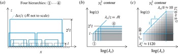However, alternative but equally valid explanations may exist for the empirically observed trends of the $\unicode[STIX]{x1D6FE}_{L}^{2}$ isocontours. Four discrete successive hierarchies of randomly positioned attached eddies are drawn in $(x,z)$ -space in figure 3(a), with each consecutive hierarchy being subject to a doubling in self-similar size and a halving of the number of eddies in this two-dimensional plane (it should be noted that the typical forward-leaning nature of the structures is neglected since a consistent phase shift is irrelevant in the context of the LCS; see 3.1). Self-similarity implies that each eddy hierarchy is associated with the same ratio of the minimum streamwise wavelength at which energetic variance still appears relative to its wall-normal extent. We refer to this ratio as the streamwise/wall-normal aspect ratio, denoted as  Due to the streamwise repetition of eddies associated with one specific hierarchy, say ones with a wall-normal extent of $z=l$ , energetic variance may appear for all scales larger than the smallest energetic scale, e.g. energy appears for  Therefore, for hierarchy 

 with a wall-normal extent of $2^{(i-1)}l$ , a non-zero coherence in $(\unicode[STIX]{x1D706}_{x},z)$ -space appears for $z<2^{(i-1)}l$ and  (see figure 3 b). The energy spectrum of the streamwise velocity fluctuations corresponding to one hierarchy of attached-eddy structures is likely non-uniform with $\unicode[STIX]{x1D706}_{x}$ and may depend on the $z$ position within the hierarchy. The magnitude of $\unicode[STIX]{x1D6FE}_{L}^{2}$ (the coherence between two locations separated in the wall-normal direction) may also vary with $\unicode[STIX]{x1D706}_{x}$ and $z$ (relative to $z_{R}$ ). That is, the coherence may depend on $\unicode[STIX]{x1D706}_{x}$ within that particular hierarchy of eddies, and within the wall-normal range spanned by the hierarchy, the coherence with the wall may vary. However, for simplicity, we idealize a uniform coherence magnitude in figure 3(b), e.g. the coherence magnitude for one hierarchy is drawn with a uniform greyscale. It should be noted that even if the coherence magnitude for one hierarchy is non-uniform, we would still obtain the same final structure of the reconstructed coherence spectrogram in the limit of infinite Reynolds number (a limitless increase of the number of hierarchies). When superposing each hierarchy of self-similar scales, coherence contours are additive (see hierarchies $\unicode[STIX]{x2460}$ – $\unicode[STIX]{x2463}$ in figure 3 b), as each attached-eddy structure is, on average, randomly positioned (Woodcock & Marusic Reference Woodcock and Marusic2015). When increasing the number of hierarchies to 10 in figure 3(c), the contour clearly reflects a discrete version of the smooth $\unicode[STIX]{x1D6FE}_{L}^{2}$ isocontours in figure 2(c). Within a triangular region in ( $\unicode[STIX]{x1D706}_{x},z$ )-space, bounded by a wall-normal height $z=l$ (the smallest self-similar structure in the eddy hierarchy), an inner limit (constant $\unicode[STIX]{x1D706}_{x}/z$ ) and an outer limit (constant $\unicode[STIX]{x1D706}_{x}/\unicode[STIX]{x1D6FF}$ ), the $\unicode[STIX]{x1D6FE}_{L}^{2}$ isocontours align with lines of constant $\unicode[STIX]{x1D706}_{x}/z$ (see the contours within the triangle in figure 3 c). The quantitative boundaries of this triangular region are discussed in § 3.4. Within the triangle, the magnitude of $\unicode[STIX]{x1D6FE}_{L}^{2}$ increases linearly with $\log (\unicode[STIX]{x1D706}_{x})$ (for constant $z$ ) and decreases with $\log (z)$ (for constant $\unicode[STIX]{x1D706}_{x}$ ), which is the natural artefact of a geometrically self-similar structure. Seemingly, the coherence magnitude obeys $\unicode[STIX]{x1D6FE}_{L}^{2}=C_{1x}\ln (\unicode[STIX]{x1D706}_{x})+C_{1z}\ln (z)+C_{2}$ . Since the aspect of self-similarity implies that constant $C_{1x}=-C_{1z}=C_{1}$ , the coherence magnitude within the self-similar region adheres to

Evidently, a self-similar attached-eddy structure is ingrained within the TBL flow where the wall-coherent structure is described by (3.2); its universality is examined in § 3.4. It should be noted that the sole dependence of $\unicode[STIX]{x1D6FE}_{L}^{2}$ on $\unicode[STIX]{x1D706}_{x}/z$ follows a similarity hypothesis already proposed by Davenport (Reference Davenport1961) in an investigation of the square-root coherence, $\unicode[STIX]{x1D6FE}_{L}$ , in meteorological boundary layers. Morrison & Kronauer (Reference Morrison and Kronauer1969) studied the same similarity hypothesis in pipe flow, which Bullock, Cooper & Abernathy (Reference Bullock, Cooper and Abernathy1978) supported via two-point radial correlations of turbulence in narrow frequency bands. del Álamo et al. (Reference del Álamo, Jiménez, Zandonade and Moser2004) used the square-root coherence between two wall-normal locations as a function of both streamwise and spanwise wavelengths to also highlight an ‘attached’ self-similar structure.

Figure 4.

Coherence and energy spectrograms, following $\unicode[STIX]{x1D6FE}_{L}^{2}(z,z_{R};\unicode[STIX]{x1D706}_{x})$ (levels: 0.1 : 0.1 : 0.9) and $k_{x}\unicode[STIX]{x1D719}_{uu}(z;\unicode[STIX]{x1D706}_{x})/U_{\unicode[STIX]{x1D70F}}^{2}$ (levels: 0.2 : 0.2 : 1.8) for all datasets listed in table 1. The triangles (and the regions identified with the dashed lines) are described in § 3.4 (it should be noted that the inner and outer limits of the triangle are listed in panel a).

3.3 Remarks about spanwise resolutions and temporal data limitations

Coherence spectrograms for all data listed in table 1 are shown in figure 4 (in the same way as in figure 2 c). A comparison of datasets ${\mathcal{S}}_{1}$ and ${\mathcal{S}}_{2}$ (figure 4 a,c) demonstrates that coarser spanwise resolutions (at least to the same degree as the laboratory experiments, simulated by ${\mathcal{S}}_{2}$ ) do not affect the coherence spectrograms in our region of interest ( $z^{+}\gtrsim 80$ per our discussion later on). The decrease in coherence for the filtered data ${\mathcal{S}}_{2}$ , in close proximity to $z_{R}$ , is an artefact of the different $\unicode[STIX]{x0394}y$ resolutions of the $z$ range and $z_{R}$ reference data (table 1). From figure 4(b,d), it can be concluded that the frequency attenuation in the hotfilm reference signal of ${\mathcal{E}}_{1}$ – compared with the hotwire reference of ${\mathcal{E}}_{2}$ – does not affect the coherence spectrogram. This insensitivity to spectral attenuation (or amplification) is an inherent advantage of the per-scale normalization in (3.1). Two-point correlation coefficients in the physical domain are fundamentally different in this regard, since the normalization utilizes the root mean square of all fluctuations via $\unicode[STIX]{x1D70C}_{uu}(z,z_{R},\unicode[STIX]{x1D70F})={\mathcal{F}}^{-1}[\unicode[STIX]{x1D719}_{uu}^{\prime }(z,z_{R};\unicode[STIX]{x1D706}_{x})]/[u_{rms}(z)u_{rms}(z_{R})]$ . As such, $\unicode[STIX]{x1D70C}_{uu}$ will differ for ${\mathcal{E}}_{1}$ and ${\mathcal{E}}_{2}$ since $u_{rms}(z_{R})$ of the attenuated hotfilm sensor signal includes more coherent energy (relative to the total resolved energy) in comparison to the hotwire reference signal ( ${\mathcal{E}}_{2}$ ). Even though phase information is embedded within the two-point correlation coefficient via the time shift $\unicode[STIX]{x1D70F}$ , a scale-dependent phase may also be considered directly from the complex cross-spectrum $\unicode[STIX]{x1D719}_{uu}^{\prime }$ (e.g. Baars, Hutchins & Marusic Reference Baars, Hutchins and Marusic2016; Baars et al. Reference Baars, Hutchins and Marusic2017). A noticeable difference in $\unicode[STIX]{x1D6FE}_{L}^{2}$ from datasets ${\mathcal{S}}_{2}$ , ${\mathcal{E}}_{2}$ and ${\mathcal{E}}_{3}$ (figure 4 c,d) is the vanishing coherence in temporal data ( ${\mathcal{E}}_{2}$ ), compared with spatial data ( ${\mathcal{S}}_{2}$ ), for $\unicode[STIX]{x1D706}_{x}^{+}\lesssim 7000$ . Recently, Baars et al. (Reference Baars, Hutchins and Marusic2017) showed that the characteristic temporal frequency of the small scales (generally $\unicode[STIX]{x1D706}_{x}^{+}<7000$ ) exhibits an enhanced large-scale (e.g. $\unicode[STIX]{x1D706}_{x}^{+}>7000$ ) modulation in comparison with the spatial frequency modulation. This strengthening arguably arises from a varying convection velocity of the small scales via $U_{c}(z,t)\propto [U(z)+u_{L}(z,t)]^{1/2}$ ( $u_{L}$ is the large-scale velocity), which to a fixed-observer sensor appears as an additional modulation to the already spatially modulated scales. Since this effect is driven by the amplitude of $u_{L}$ (varying in $z$ and time), the modulation is inconsistent across $z$ and therefore suppresses the phase-consistent coherence.

Figure 5.

(a) Coherence spectrogram of dataset ${\mathcal{E}}_{2}$ (with the wavelength axis predivided by $z$ ). The thicker portions of the curves correspond to $3Re_{\unicode[STIX]{x1D70F}}^{1/2}<z^{+}<0.15Re_{\unicode[STIX]{x1D70F}}$ and $20z<\unicode[STIX]{x1D706}_{x}<6\unicode[STIX]{x1D6FF}$ . It should be noted that the inclined plane with the solid boundary (bounded by $\unicode[STIX]{x1D6FE}_{L}^{2}=1$ ) reflects (3.2) with $C_{1}\approx 0.302$ and $C_{2}\approx -0.796$ determined from fitting (3.2) to the thick portions of the coherence spectra. Relation (3.2) has a region of validity bounded by an inner limit of $\unicode[STIX]{x1D706}_{x}/z\approx 14$ , an outer limit of $\unicode[STIX]{x1D706}_{x}/\unicode[STIX]{x1D6FF}\approx 10$ and a wall-normal height of $z^{+}=80$ (this region is also indicated in figure 4 d). (b) Linear coherence spectra $\unicode[STIX]{x1D6FE}_{L}^{2}(z,z_{R};\unicode[STIX]{x1D706}_{x})$ for all datasets listed in table 1 for wall-normal positions within the range $3Re_{\unicode[STIX]{x1D70F}}^{1/2}<z^{+}<0.15Re_{\unicode[STIX]{x1D70F}}$ .

3.4 Universality of self-similar wall-attached eddies

As reasoned in the lead-up to (3.2), the coherence is anticipated to be a sole function of $\unicode[STIX]{x1D706}_{x}/z$ in a triangular region bounded by $z=l$ , an inner limit $\unicode[STIX]{x1D706}_{x}/z$ and an outer limit $\unicode[STIX]{x1D706}_{x}/\unicode[STIX]{x1D6FF}$ . We here perform a fit of (3.2) to dataset ${\mathcal{E}}_{2}$ , since its corresponding coherence spectrogram contains a larger self-similar range in the logarithmic region than its DNS counterparts (datasets ${\mathcal{S}}_{1}$ and ${\mathcal{S}}_{2}$ ) and captures all energy in the largest scales (the large scales in the atmospheric surface layer data, ${\mathcal{E}}_{3}$ , were affected by filtering procedures to eliminate variations in the free-stream velocity; see Marusic & Heuer Reference Marusic and Heuer2007; Hutchins et al. Reference Hutchins, Chauhan, Marusic and Klewicki2012). All $\unicode[STIX]{x1D6FE}_{L}^{2}$ -spectra from dataset ${\mathcal{E}}_{2}$ (used in creating the isocontour in figure 4 d) are replotted in figure 5(a) with the wavelength axis predivided by $z$ . To fit (3.2) to the coherence spectra – and thus determine $C_{1}$ and $C_{2}$ – we select portions of the spectra within the logarithmic region, taken as $3Re_{\unicode[STIX]{x1D70F}}^{1/2}<z^{+}<0.15Re_{\unicode[STIX]{x1D70F}}$ (Marusic et al. Reference Marusic, Monty, Hultmark and Smits2013), and within a region bounded by inner and outer limits, $20z<\unicode[STIX]{x1D706}_{x}<6\unicode[STIX]{x1D6FF}$ (chosen by visual inspection). These portions are highlighted with thicker curves in figure 5(a) and are surrounded by the dashed lines indicating the bounds. It should be noted that these bounds for fitting (3.2) are redrawn on all panels in figure 4 for reference, and that the choice of lower limit $z^{+}=3Re_{\unicode[STIX]{x1D70F}}^{1/2}$ avoids the region where the spatial/temporal coherence discrepancy was observed (§ 3.3). A linear least squares fitting of (3.2) to the $\unicode[STIX]{x1D6FE}_{L}^{2}$ -spectra of ${\mathcal{E}}_{2}$ in the fitting region results in $C_{1}\approx 0.302$ and $C_{2}\approx -0.796$ . The corresponding surface represented by (3.2) is shown with the inclined triangular plane in figure 5(a) and is bounded by $\unicode[STIX]{x1D6FE}_{L}^{2}=1$ . Now, the inner-scaling limit of this plane may be taken as the $\unicode[STIX]{x1D706}_{x}/z$ value for which $\unicode[STIX]{x1D6FE}_{L}^{2}=0$ (see § 3.2); note this simultaneously exposes the aspect ratio of a self-similar attached-eddy structure. Hence, we obtain a stochastic streamwise/wall-normal aspect ratio of

indicated by the solid boundary of the triangle in the $\unicode[STIX]{x1D6FE}_{L}^{2}=0$ plane in figure 5(a).

At scales beyond an outer limit $\unicode[STIX]{x1D706}_{x}/\unicode[STIX]{x1D6FF}$ , the coherence is scale-independent, as is observed in figure 5(a). It should be noted that these scales are not part of the (3.2)-compatible self-similarity, because self-similar growth of these structures in $z$ is bounded by the boundary layer thickness; this results in scale-independent contours of $\unicode[STIX]{x1D6FE}_{L}^{2}$ (see the conceptual reconstruction of the coherence magnitude in figure 3 c). From (3.2), it follows that the scale-independent coherence should now adhere to $\unicode[STIX]{x1D6FE}_{L}^{2}=-C_{1}\ln (z)+C_{3}$ . This equation is fitted to the data of ${\mathcal{E}}_{2}$ within the range $0.07<z/\unicode[STIX]{x1D6FF}<0.50$ (plateau values of $\unicode[STIX]{x1D6FE}_{L}^{2}$ are indicated with the open circles in the $\unicode[STIX]{x1D706}_{x}/z=10^{4}$ plane in figure 5 a). The fit, indicated with the dashed line in the $\unicode[STIX]{x1D706}_{x}/z=10^{4}$ plane, intersects $\unicode[STIX]{x1D6FE}_{L}^{2}=0$ at $z/\unicode[STIX]{x1D6FF}\approx 0.710$ . Judiciously, an outer-scaling limit for (3.2) may be taken as  and represents the transition in the coherence from a self-similar scaling via (3.2) to a scale-independent trend at $\unicode[STIX]{x1D706}_{x}/\unicode[STIX]{x1D6FF}\gg 10$ . Vassilicos et al. (Reference Vassilicos, Laval, Foucaut and Stanislas2015) emphasized that an outer-scaling limit is required for modelling suitable subranges in $(\unicode[STIX]{x1D706}_{x},z)$ -space where the spectral energy density adheres to the AEH; our identified limit of $\unicode[STIX]{x1D706}_{x}/\unicode[STIX]{x1D6FF}\approx 10$ supports this.

Finally, regarding the wall-normal extent $l$ of the smallest eddying motions in the self-similar hierarchy, results (not explicitly shown) suggest that $l^{+}\approx 80$ for all Reynolds numbers. It should be noted that a Reynolds-number dependence in the lower limit of a logarithmic layer, such as the ${\sim}Re_{\unicode[STIX]{x1D70F}}^{1/2}$ dependence (Klewicki et al. Reference Klewicki, Fife and Wei2009), may be equally valid but is simply dependent on what types of motions are included in an analysis, namely self-similar or non-self-similar motions. Recent support for self-similar behaviour down to $l^{+}\approx 80$ was presented by Agostini & Leschziner (Reference Agostini and Leschziner2017) through examining subranges in ( $\unicode[STIX]{x1D706}_{x},z$ )-space of isotropic (associated with detached eddies) and anisotropic scales (associated with attached eddies) in $Re_{\unicode[STIX]{x1D70F}}\approx 4200$ channel flow. A lower bound for the validity of (3.2) cannot be deduced by fitting a proposed relation to the coherence spectra. First of all, the spatial/temporal coherence discrepancy affects the $\unicode[STIX]{x1D6FE}_{L}^{2}$ -spectra of dataset ${\mathcal{E}}_{2}$ at $z^{+}\lesssim 3Re_{\unicode[STIX]{x1D70F}}^{1/2}$ (see § 3.3). Second, within the near-wall region, the coherence spectra are not only influenced by a self-similar wall-attached structure but also by the strong coherent near-wall streaks. This is particularly clear from the high magnitude of the coherence in the spatial DNS dataset, ${\mathcal{S}}_{1}$ , shown in figure 4(a).

To summarize the expected region of validity of (3.2), we drew a triangular plane in figure 5(a) with a lower limit of $z^{+}=80$ , an inner-scaling limit of  and an outer-scaling limit of $\unicode[STIX]{x1D706}_{x}/\unicode[STIX]{x1D6FF}\approx 10$ (it should be noted that the coherence is bounded by $\unicode[STIX]{x1D6FE}_{L}^{2}=1$ ). The same triangular region is drawn on all panels in figure 4 (with the bounds summarized in figure 4 a). Intriguingly, the coherence spectrograms of the DNS data ( ${\mathcal{S}}_{1}$ and ${\mathcal{S}}_{2}$ ) and atmospheric surface layer data ( ${\mathcal{E}}_{3}$ ) in figure 4(a,c) appear to adhere to these inner- and outer-scaling limits determined from dataset ${\mathcal{E}}_{2}$ (similarly for dataset ${\mathcal{E}}_{1}$ in figure 4 b, although this is expected due to the almost identical Reynolds number between ${\mathcal{E}}_{1}$ and ${\mathcal{E}}_{2}$ ). To inspect the universality of (3.2) further, all $\unicode[STIX]{x1D6FE}_{L}^{2}$ -spectra within the range $3Re_{\unicode[STIX]{x1D70F}}^{1/2}<z^{+}<0.15Re_{\unicode[STIX]{x1D70F}}$ (the same wall-normal range as used for fitting (3.2)) are plotted as a function of $\unicode[STIX]{x1D706}_{x}/z$ in figure 5(b). A simultaneous increase in the greyscale and decrease in the line thickness indicates an increasing $z$ location of the coherence spectra. Relation (3.2), with $C_{1}$ and $C_{2}$ solely determined from dataset ${\mathcal{E}}_{2}$ , is superposed on all data. By inspection, we observe that the $Re_{\unicode[STIX]{x1D70F}}\approx 2000$ data from DNS contain the same self-similar streamwise/wall-normal structure of wall-attached turbulence as found in the laboratory ( $Re_{\unicode[STIX]{x1D70F}}\approx 14\,000$ ) and atmospheric data ( $Re_{\unicode[STIX]{x1D70F}}\approx 1.4\times 10^{6}$ ). This furthermore suggests the universality of (3.2) with constants $C_{1}\approx 0.302$ and $C_{2}\approx -0.796$ , and the associated region of validity drawn in figure 4.

Finally, in the context of self-similar structure identified in DNS of turbulent channel flow, our universal streamwise/wall-normal aspect ratio of  resides between two distinct self-similar components, described by Hwang (Reference Hwang2015) as long streaky structures ( $\unicode[STIX]{x1D706}_{x}/z\simeq 100$ ) and shorter vortex packet-type structures ( $\unicode[STIX]{x1D706}_{x}/z\simeq 3\sim 6$ ). Hwang’s observations are consistent with earlier work by, for instance, del Álamo et al. (Reference del Álamo, Jiménez, Zandonade and Moser2006). The self-similar components in DNS data have typically been extracted via asymptotic behaviours seen in unfiltered energy (co)spectra of velocities, which may obscure an underlying self-similarity (see § 1). del Álamo et al. (Reference del Álamo, Jiménez, Zandonade and Moser2004) showed, using the square-root coherence, that an inner limit of $\unicode[STIX]{x1D706}_{x}/z\approx 10$ separates the wall-attached and wall-detached eddies, closely resembling (3.3).