1 Introduction
As an important mechanism of heat transfer in fluids, Rayleigh–Bénard convection (RBC) has been studied extensively in the past (e.g. Ahlers, Grossmann & Lohse Reference Ahlers, Grossmann and Lohse2009). One new aspect of such studies is thermally induced fluid–structure interaction, where buoyancy-driven flow interacts with the solid body and passes momentum through fluid forces. Periodic motions and limit cycles are observed in thermally driven systems – for example in Zhang & Libchaber (Reference Zhang and Libchaber2000), a plate floating on top of convective fluid undergoes periodic motion between boundaries. Plate tectonics in geodynamics is another example but on a larger scale. Theories suggest that the continental motion is due to the convection in the mantle of Earth (see Turcotte & Schubert Reference Turcotte and Schubert2002), and this theory has been explored both experimentally (Elder Reference Elder1968; Howard, Malkus & Whitehead Reference Howard, Malkus and Whitehead1970; Whitehead Reference Whitehead1972) and numerically (Gurnis Reference Gurnis1988; Gurnis & Zhong Reference Gurnis and Zhong1991; Lowman & Jarvis Reference Lowman and Jarvis1993, Reference Lowman and Jarvis1995; Whitehead & Behn Reference Whitehead and Behn2015). Another example is self-propulsion through natural convection (Allshouse, Barad & Peacock Reference Allshouse, Barad and Peacock2010; Mercier et al. Reference Mercier, Ardekani, Allshouse, Doyle and Peacock2014), where an inclined heated surface induces upward buoyancy flow and propels itself through the counterforce generated by the fluid.
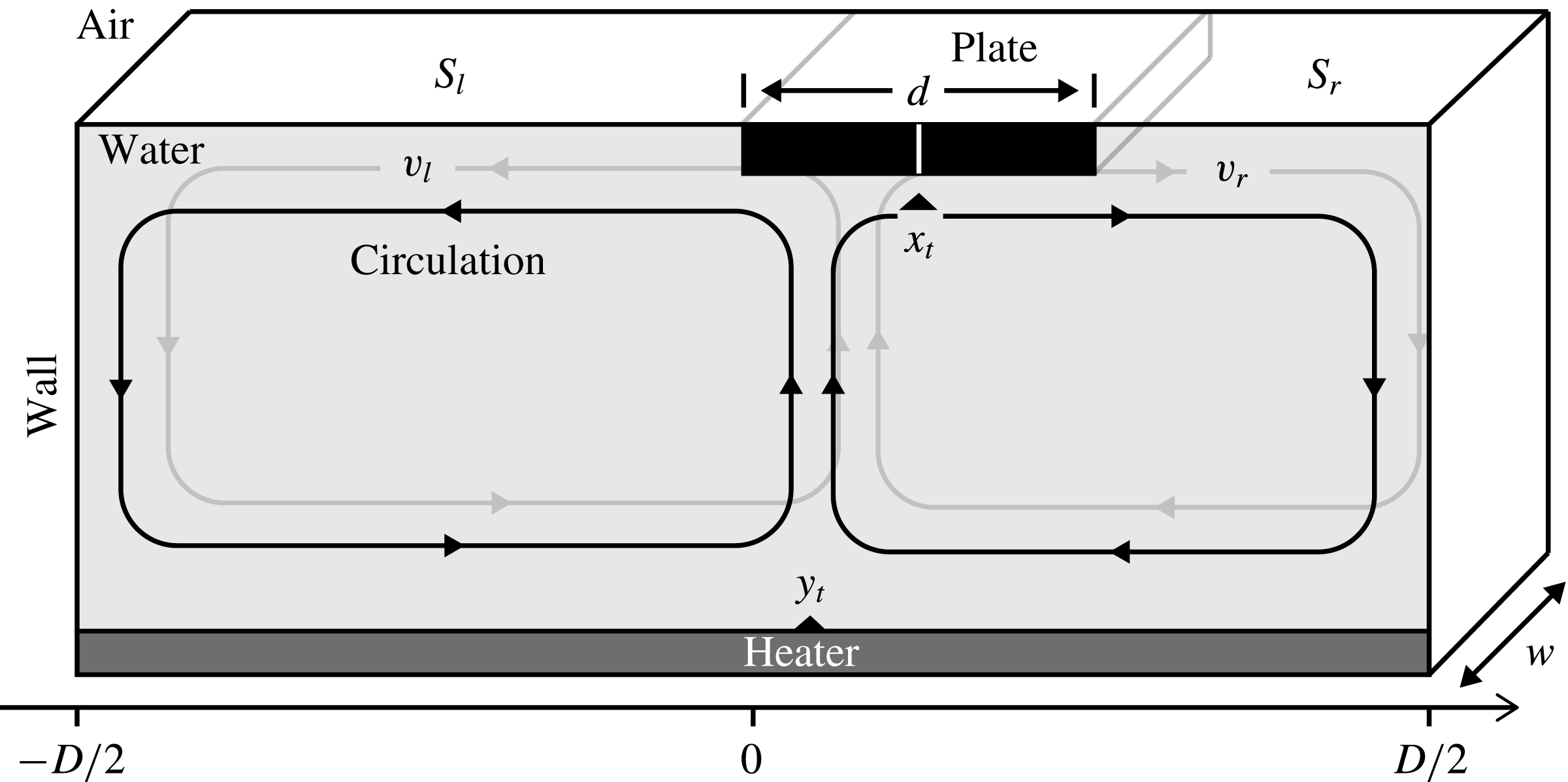
Schematic of the system. A floating plate with size
 $d$
is free to move horizontally on convective fluid in a rectangular tank. The fluid is heated from below and cooled from above, undergoing Rayleigh–Bénard convection and exerting a fluid force on the plate (centre at
 $x_{t}$
). Upwelling flow rises from the location
 $y_{t}$
and separates into two large-scale circulations that have velocity
 $v_{l},v_{r}$
to the left and right, respectively.

Zhong and Zhang have experimentally studied the interaction between convective fluid and a floating plate on the free surface (Zhang & Libchaber Reference Zhang and Libchaber2000; Zhong & Zhang Reference Zhong and Zhang2005, Reference Zhong and Zhang2007a
,Reference Zhong and Zhang
b
). In their experiment, the authors considered an elongated water tank of length
 $D$
and width
 $w$
, as shown in figure 1, where the fluid within is heated uniformly from the bottom and cooled at the open surface. In their experiments, the Rayleigh number
 $Ra=1.1\times 10^{9}$
and the Prandtl number
 $Pr=4.4$
, which yield a Reynolds number
 $Re\sim 3000$
in the bulk. Structures such as thermal plumes are formed and their collective motion forms the large-scale circulation (Krishnamurti & Howard Reference Krishnamurti and Howard1981; Ahlers et al.
Reference Ahlers, Grossmann and Lohse2009). The turbulent aspects of convective fluid, especially with the presence of large-scale circulation, have been modelled as noise in the past (Sreenivasan, Bershadskii & Niemela Reference Sreenivasan, Bershadskii and Niemela2002; Benzi Reference Benzi2005; Brown, Nikolaenko & Ahlers Reference Brown, Nikolaenko and Ahlers2005; Zhong, Sterl & Li Reference Zhong, Sterl and Li2015), and well-developed tools such as the Kolmogorov equations can then be utilized to analyse the stochastic processes involved in RBC. However, when fluid–structure interaction is involved, the existence of solid boundaries complicates the analysis and new mathematical tools are required.
Floating on the open surface, a free-moving plate of length
 $d$
is subject to the net viscous force from the fluid motion underneath. This mobile plate is free to move along the horizontal direction, with walls on each side of the tank as the limiting boundary. Intriguing dynamics are observed in the experiments, where two states of plate motion exist: when the plate size is smaller than a critical value
 $d_{c}=0.58D$
(Zhong & Zhang Reference Zhong and Zhang2007b
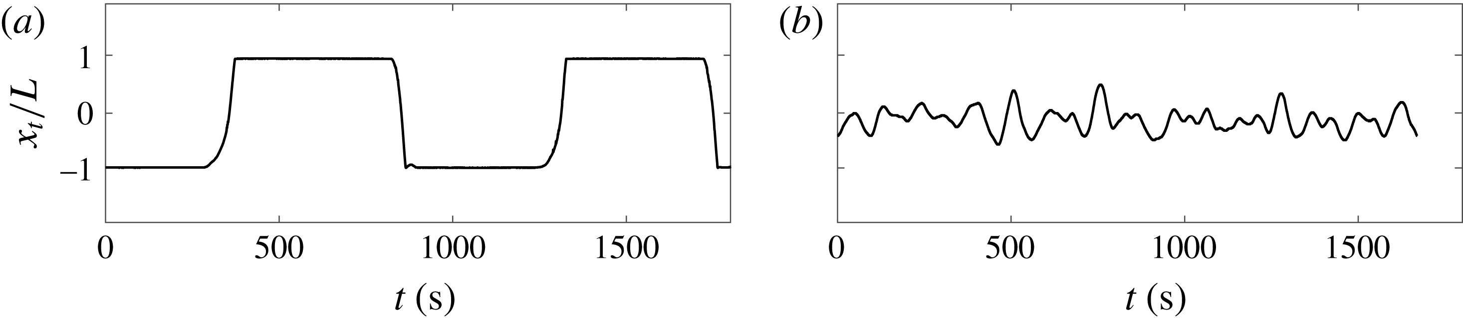
), the plate oscillates between two sides of the tank; as the plate size increases beyond this critical value, the plate becomes trapped in the middle of the tank. Two typical trajectories are presented in figure 2.
Zhong and Zhang also derived a model (ZZ model) in terms of a piecewise smooth dynamical system that incorporates the force balance and the ‘thermal blanket effect’ (Zhang & Libchaber Reference Zhang and Libchaber2000; Zhong & Zhang Reference Zhong and Zhang2005, Reference Zhong and Zhang2007a
,Reference Zhong and Zhang
b
). This model explains the existence of two states and provides an explanation of
 $d_{c}$
. However, the ZZ model cannot recover any stochastic features observed in the experiment due to its deterministic nature. In reality, the convective fluid is in a turbulent state that generates random forces on the plate, and it is clear that the plate undergoes stochastic motion, as shown in figure 2(b).
Our current work will further advance the ZZ model to a novel variational inequality. Furthermore, in the presence of random fluctuations, the problem becomes a stochastic variational inequality (SVI) whose solution is a continuous (degenerate) reflected diffusion. This type of problem has been studied in the past by Bensoussan et al. (Reference Bensoussan, Mertz, Pironneau and Turi2009), Bensoussan & Mertz (Reference Bensoussan and Mertz2012), Mertz & Feau (Reference Mertz and Feau2012), Laurière & Mertz (Reference Laurière and Mertz2015), Mertz & Bensoussan (Reference Mertz and Bensoussan2015), Bensoussan et al. (Reference Bensoussan, Mertz and Yam2016), Feau, Laurière & Mertz (Reference Feau, Laurière and Mertz2018) and Mertz, Stadler & Wylie (Reference Mertz, Stadler and Wylie2017), as well as by Bensoussan & Turi (Reference Bensoussan and Turi2008) and Bensoussan & Turi (Reference Bensoussan and Turi2010) in the context of elasto-plastic oscillators.
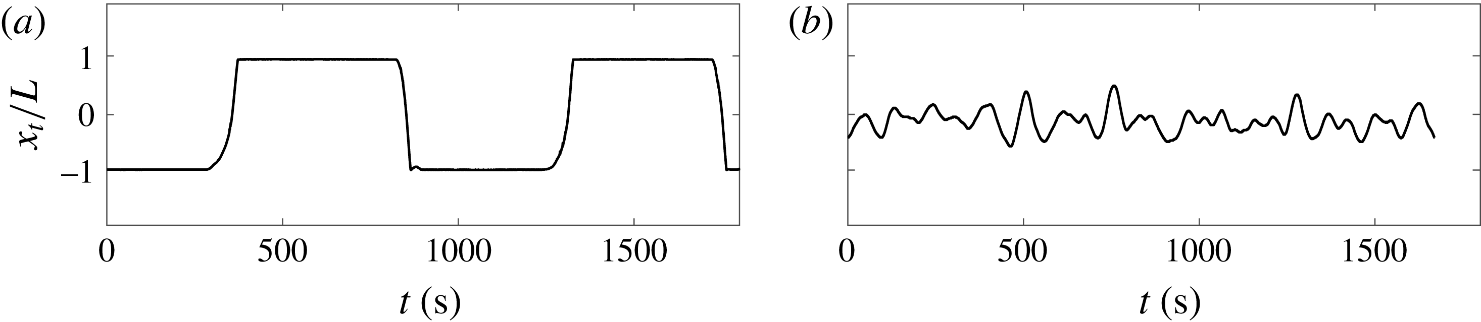
Experimental data from Zhong & Zhang (Reference Zhong and Zhang2005) and Zhong & Zhang (Reference Zhong and Zhang2007b
). The range of
 $x_{t}$
is defined as
 $L=(D-d)/2$
so
 $x_{t}\in [-L,L]$
. (a)
 $d<d_{c}$
: oscillatory state (
 $d/D=0.2$
), where the floating plate moves towards one sidewall and stays for a random but finite amount of time before moving towards the other sidewall. (b)
 $d>d_{c}$
: trapped state (
 $d/D=0.7$
), where the floating plate undergoes stochastic motion at the centre of tank without touching either sidewall.
Although our model follows along the lines of the ZZ model, the characterization of dynamical states raises completely different problems due to the stochastic nature of our model. One way to treat these problems is to employ the sophisticated (but necessary) mathematical approach based on SVIs. In terms of benefits for the modellers, the SVI approach provides a new tool to access statistics of the system that was not possible before our present work. From the SVI theory, we obtain the Kolmogorov equations that allow us to compute transition probabilities of the stochastic ZZ model, which has an advantage over other stochastic approaches.
As we will show, the good agreement between this newly developed mathematical model and the experiments suggests that the framework of SVI could have further applications in other scientific and engineering fields that involve fluid–structure interactions, where fluid forces are under temporal and/or spatial fluctuations. For example, a limit cycle exists in the geophysical process of continental drift that has been happening constantly on Earth for billions of years. The viscous force on the base of the continents changes the locations of continents in a way similar to the mechanism depicted in figure 1, and sets up the Wilson cycle of tectonic motion (Turcotte & Schubert Reference Turcotte and Schubert2002).
2 ZZ model and stochastic aspects of the experiments
A physically inspired ODE model is proposed by Zhong and Zhang (ZZ model), and it successfully captures different states of the plate motion. In the experiments, two counter-rotating circulations set up a diverging flow field centred at
 $y_{t}$
on the open surface, as shown in figure 1. Depending on its location
 $x_{t}$
, the plate is either transported by a single circulation or balanced by the diverging flow field underneath. The circulation speed
 $v_{i}$
on the open surface is observed to scale linearly with the open surface area
 $S_{i}(x_{t},y_{t})$
and can be determined as
 $v_{i}(x_{t},y_{t})=v_{0}+\unicode[STIX]{x1D703}S_{i}(x_{t},y_{t})$
, where
 $v_{0}$
and
 $\unicode[STIX]{x1D703}$
are constants and the index
 $i=(l,r)$
indicates the open surface to the left or the right. In the experiments, a delay
 $\unicode[STIX]{x1D6FF}t\approx 10$
s is also observed in the response of flow velocity to the surface area and
 $v_{i}(x_{t},y_{t})=v_{0}+\unicode[STIX]{x1D703}S_{i}(x_{t-\unicode[STIX]{x1D6FF}t},y_{t-\unicode[STIX]{x1D6FF}t})$
, which reflects the hysteretic dependence between the flow structure and the plate location. In this study, the delay is ignored due to its relative fast scale compared to other dynamics (typically approximately 5 min), so
 $S_{i}(x_{t-\unicode[STIX]{x1D6FF}t},y_{t-\unicode[STIX]{x1D6FF}t})\approx S_{i}(x_{t},y_{t})$
becomes a good approximation in our modelling. As noted in previous works (Zhong & Zhang Reference Zhong and Zhang2007b
), the plate dynamics stays unchanged for the model without the delay
 $\unicode[STIX]{x1D6FF}t$
, except for estimating the critical plate size
 $d_{c}$
, as we shall discuss later. The net fluid force on the plate can then be associated with the surface flow velocity through integrating the shear stress
 $\unicode[STIX]{x1D70F}$
over the plate surface,
 $$\begin{eqnarray}F(x_{t},y_{t})=\int _{plate}\unicode[STIX]{x1D70F}\,\text{d}S\sim \unicode[STIX]{x1D702}w/\unicode[STIX]{x1D706}\int _{x_{t}-d/2}^{x_{t}+d/2}[v_{i}(x_{t},y_{t})-{\dot{x}}_{t}]\,\text{d}x,\end{eqnarray}$$
with fluid viscosity
 $\unicode[STIX]{x1D702}$
and thermal boundary layer thickness
 $\unicode[STIX]{x1D706}$
. Due to the similar density between the plate and the fluid, the net force
 $F(x_{t},y_{t})\approx 0$
leads to the first equation in (2.2). In the experiment, the exposed fluid surface is cooled (i.e. loses heat faster) relative to the covered fluid due to the slowed heat transfer of diffusion through the plate. As a result, heat accumulates under the plate, leading to the ‘thermal blanket effect’ and a local upwelling flow which separates the two large-scale circulations. When the plate is in motion, the upwelling centre
 $y_{t}$
follows the plate with a speed that is observed to be proportional to the distance
 $x_{t}-y_{t}$
. This attraction sets the motion of
 $y_{t}$
and provides the second equation in (2.2) to close the system.
 $$\begin{eqnarray}{\dot{x}}_{t}=-U_{d}^{\prime }(x_{t};y_{t})\quad \text{and}\quad {\dot{y}}_{t}=\unicode[STIX]{x1D6FD}d(x_{t}-y_{t}),\end{eqnarray}$$
with
 $$\begin{eqnarray}U_{d}(x;y)\triangleq \frac{\unicode[STIX]{x1D6FC}(2d)}{2}x^{2}-\unicode[STIX]{x1D6FC}(d)xy,\quad \unicode[STIX]{x1D6FC}(\cdot )\triangleq \frac{\unicode[STIX]{x1D703}(\cdot -D)-2v_{0}}{d},\quad \unicode[STIX]{x1D703},v_{0},\unicode[STIX]{x1D6FD}>0.\end{eqnarray}$$
We have ignored the surface drag term that appeared in Zhong & Zhang (Reference Zhong and Zhang2007b
) by setting
 $\unicode[STIX]{x1D6FE}=0$
in their original work. It is noted that the mathematical treatment and results remain the same with or without this surface drag. The model without the surface drag simply suggests that the plate has negligible inertia and is always in equilibrium, such that the net fluid force is 0. Physical parameters
 $\unicode[STIX]{x1D703},v_{0},\unicode[STIX]{x1D6FD}$
can be either measured or estimated through experiments, and their values in Zhong & Zhang (Reference Zhong and Zhang2007b
) are
 $(\unicode[STIX]{x1D703},v_{0},\unicode[STIX]{x1D6FD})=(0.075~\text{s}^{-1},0.015D~\text{s}^{-1},0.017D^{-1}~\text{s}^{-1})$
.
It is important to emphasize that the potential
 $U_{d}$
is unidimensional with respect to the variable
 $x$
, whereas the variable
 $y$
appears only as a parameter, with the notation
 $^{\prime }$
representing the derivative with respect to
 $x$
. To describe the interaction with the walls, let us cite a passage of Zhong & Zhang (Reference Zhong and Zhang2007b
):

Physically, the experiment is designed so that the contact between the plate and sidewall is below the fluid–air interface, so the surface tension does not contribute to the boundary interaction and the plate can detach once the sign of
 $U_{d}$
is reversed. In the remainder of this study,
 $L\triangleq (D-d)/2$
so
 $x_{t}\in [-L,L]$
and
 $y_{t}\in \mathbb{R}$
(
 $y_{t}$
is not constrained but remains bounded in
 $[-D/2,D/2]$
from its own dynamics).
The boundary motion can then be classified into two states according to the shape of the potential in which
 $x$
evolves, and a direct calculation shows that
 $U_{d}^{^{\prime \prime }}(x;y)=\unicode[STIX]{x1D6FC}(2d)$
, which determines the convexity of
 $U_{d}$
with respect to the direction
 $x$
. Thus defining
 $d_{c}\triangleq D/2+v_{0}/\unicode[STIX]{x1D703}$
such that
 $U_{d_{c}}^{^{\prime \prime }}(x;y)=\unicode[STIX]{x1D6FC}(2d_{c})=0$
, the following properties hold:
(i) if
 $d=d_{c}$
,
$\unicode[STIX]{x1D6FC}(2d_{c})=0$
at criticality, and this is the intermittent state,
(ii) if
$d<d_{c}$
then
$\unicode[STIX]{x1D6FC}(2d)<0$
, the potential is concave and leads to an oscillatory state,(iii) if
$d>d_{c}$
then
$\unicode[STIX]{x1D6FC}(2d)>0$
, the potential is convex and leads to a trapped state.


In Zhong & Zhang (Reference Zhong and Zhang2007b
), the original ZZ model suggests
 $d_{c}=0.58D$
, which accurately captured the critical behaviour. However in our model, the value
 $d_{c}=D/2+v_{0}/\unicode[STIX]{x1D703}=0.7D$
is overestimated without the presence of the delay term
 $\unicode[STIX]{x1D6FF}t$
.
In figure 2(b), the stochastic motion of the floating plate is driven by fluctuations in the large-scale circulation, where thermal plumes arrive at the floating plate at random. Due to the stochastic movement of the plume centre
 $y_{t}$
, the speed and arrival time of thermal plumes is random and the floating boundary experiences stochastic forcing. This randomness of flow structure inspires us to impose a white noise
 $\unicode[STIX]{x1D70E}{\dot{w}}_{t}$
on the motion of the plumes centre
 $y_{t}$
, and (2.2) can be stochastically extended as
 $$\begin{eqnarray}{\dot{x}}_{t}=-U_{d}^{\prime }(x_{t};y_{t})\quad \text{and}\quad {\dot{y}}_{t}=\unicode[STIX]{x1D6FD}d(x_{t}-y_{t})+\unicode[STIX]{x1D70E}{\dot{w}}_{t}.\end{eqnarray}$$
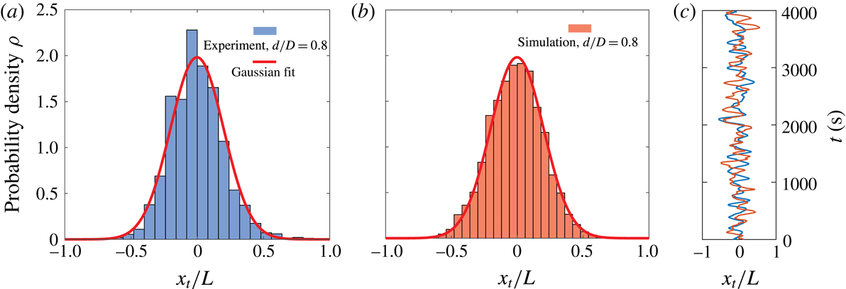
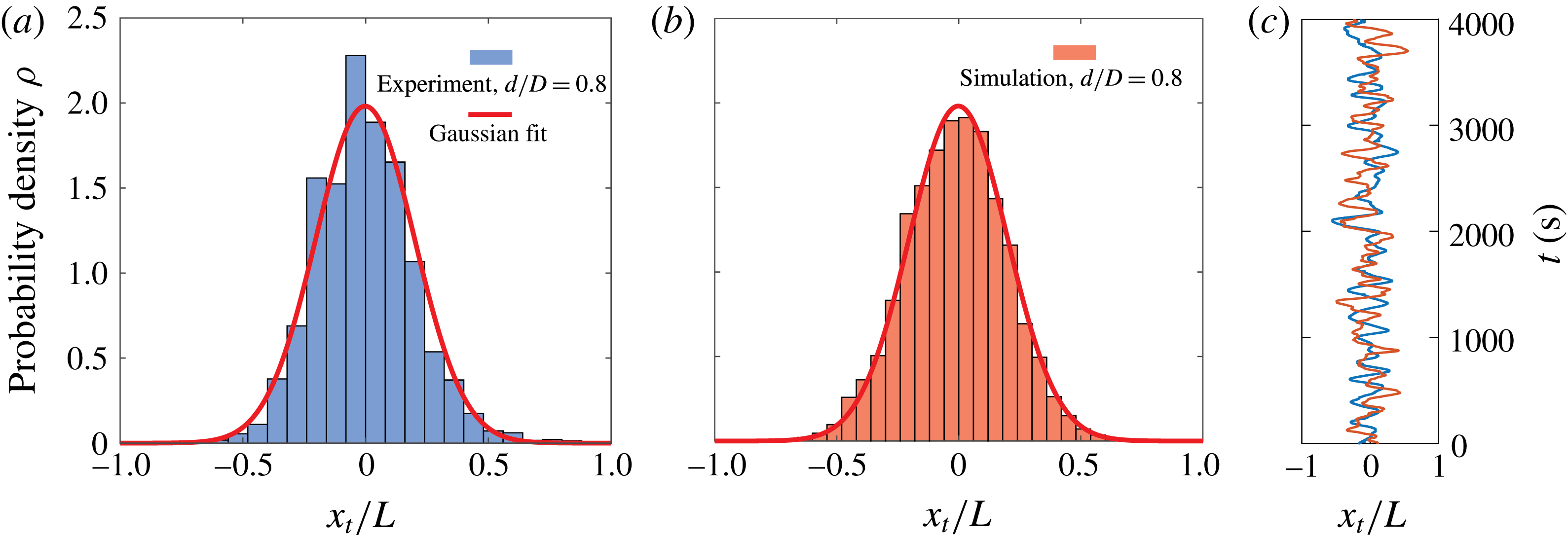
PDF and trajectory of the plate centre
 $x_{t}/L$
in a trapped state (
 $d/D=0.8$
). (a) Histogram of
 $x_{t}$
from the experiment. A Gaussian distribution is fitted to the data, the mean is near
 $m=0$
and standard deviation is
 $\unicode[STIX]{x1D70E}_{x}=0.20$
. (b) SDE simulation. The noise in stochastic model is estimated from the experimental data. (c) Trajectories corresponding to (a,b).
In a trapped state (
 $d>d_{c}$
),
 $x_{t}$
undergoes stochastic motion without reaching the boundary, and with the structure of (2.4) one can conclude that
 $x_{t}$
must have a Gaussian invariant distribution. Indeed this can be seen in figure 3(a), where the histogram of
 $x_{t}$
in a trapped state (
 $d/D=0.8$
) is plotted, and a Gaussian distribution fits well to the experimental data. Knowing the structure of (2.4), the strength of noise
 $\unicode[STIX]{x1D70E}$
could be estimated with the standard deviation
 $\unicode[STIX]{x1D70E}_{x}$
of
 $x_{t}$
,
 $$\begin{eqnarray}\unicode[STIX]{x1D70E}=\unicode[STIX]{x1D70E}_{x}\sqrt{2\unicode[STIX]{x1D6FD}d\frac{\unicode[STIX]{x1D6FC}(2d)}{\unicode[STIX]{x1D6FC}(d)^{2}}[\unicode[STIX]{x1D6FC}(2d)+\unicode[STIX]{x1D6FD}d]-2\unicode[STIX]{x1D6FD}d\frac{\unicode[STIX]{x1D6FD}d+\unicode[STIX]{x1D6FC}(2d)}{\unicode[STIX]{x1D6FC}(d)}}.\end{eqnarray}$$
From the experimental trajectory of
 $d=0.8D$
, we found
 $\unicode[STIX]{x1D70E}=0.001$
. Numerically solving (2.4) with
 $\unicode[STIX]{x1D70E}=0.001$
yields a PDF and a trajectory shown in figure 3(b,c), which shows a good agreement with the experiment. This estimation of noise is only valid for the trapped states, where the ZZ model behaves linearly without boundary effects.
3 Mathematical formulation of (stochastic) variational inequality
We can interpret the boundary condition
 $({\mathcal{B}}{\mathcal{C}})$
and (2.2) as follows: the sum of (a) the variation of displacement of the floating boundary, (b) the variation of flow forcing to the plate and (c) the variation of the forces from the wall interaction is 0. That is
 $$\begin{eqnarray}\text{for all }t_{0}<t_{1},\quad \underbrace{x_{t_{1}}-x_{t_{0}}}_{(a):\;\text{displacement}}=\underbrace{-\int _{t_{0}}^{t_{1}}U_{d}^{\prime }(x_{s};y_{s})\,\text{d}s}_{(b):\;\text{flow}}\underbrace{-(k_{t_{1}}-k_{t_{0}})}_{(c):\;\text{wall}}.\end{eqnarray}$$
To better understand
 $k(\cdot )$
(
 $k$
is a time-dependent function), consider the special case of a unilateral constraint
 $x_{t}\leqslant L$
in the sense that the left extremity of the water tank would be located at
 $x=-\infty$
while the right extremity would remain at
 $L$
. Then, there is an explicit expression for
 $k_{t}$
, that is
 $$\begin{eqnarray}k_{t}=\max _{0\leqslant s\leqslant t}\left(x_{0}-\int _{0}^{s}U_{d}^{\prime }(x_{s};y_{s})\,\text{d}s-L\right)^{+},\quad u^{+}\triangleq \max (0,u).\end{eqnarray}$$
Roughly speaking,
 $\text{d}k_{t}$
‘absorbs’ the part of the flow forces that would push
 $x_{t}$
beyond the wall. The bilateral constraint case,
 $|x_{t}|\leqslant L$
, belongs to the class of the so-called Skorokhod problem – see for instance Lions & Sznitman (Reference Lions and Sznitman1984) and references therein. Adapted to the present problem, it states that for
 $f_{t}\triangleq x_{0}-\int _{0}^{t}U_{d}^{\prime }(x_{s};y_{s})\,\text{d}s\in {\mathcal{C}}([0,\infty );\mathbb{R})$
with
 $|x_{0}|\leqslant L$
, there exists a unique solution
 $(x_{t},k_{t})$
of the Skorokhod problem:
 $$\begin{eqnarray}\left\{\begin{array}{@{}l@{}}x\in {\mathcal{C}}([0,\infty );[-L,L]),\quad k\in {\mathcal{C}}([0,\infty );\mathbb{R}),\quad \\ k\text{ is the sum of two monotonic functions}\quad \\ \text{and }x+k=f.\quad \end{array}\right.\end{eqnarray}$$
Precisely,
 $$\begin{eqnarray}k_{t}=\int _{0}^{t}\max (0,-U_{d}^{\prime }(L,y_{s}))\mathbf{1}_{\{x_{s}=L\}}\,\text{d}s+\int _{0}^{t}\min (0,-U_{d}^{\prime }(-L,y_{s}))\mathbf{1}_{\{x_{s}=-L\}}\,\text{d}s.\end{eqnarray}$$
The last condition means that
 $k_{t}$
is increasing, decreasing or constant when
 $x_{t}=L$
,
 $x_{t}=-L$
or
 $|x_{t}|<L$
, respectively. It is consistent with the description of the wall interaction of the ZZ model since
 $\mp U_{d}^{\prime }(x_{t};y_{t})\geqslant 0$
when
 $x_{t}=\pm L$
.
In this problem, the constraint is given by an interval (convex in
 $\mathbb{R}$
) and thus it can be recast in terms of a variational inequality (VI) (Bensoussan & Lions Reference Bensoussan and Lions1982) as follows:
 $$\begin{eqnarray}\text{for all }t\geqslant 0,\quad |x_{t}|\leqslant L,\quad \text{for all }|\unicode[STIX]{x1D709}|\leqslant L,\quad ({\dot{x}}_{t}+U_{d}^{\prime }(x_{t};y_{t}))(\unicode[STIX]{x1D709}-x)\geqslant 0.\end{eqnarray}$$
Let us emphasize that, without fluctuations,
 ${\dot{y}}_{t}=\unicode[STIX]{x1D6FD}d(x_{t}-y_{t})$
indicates that
 $y_{t}$
remains in
 $[-D/2,D/2]$
by its own dynamics. Necessarily,
 $\pm {\dot{y}}_{t}\leqslant 0$
when
 $x_{t}=\pm L$
and
 $|y_{t}|\geqslant L$
.
The VI above is an interesting interpretation as it is one way to show that the ZZ model is well-posed in terms of
 $x$
and
 $y$
only, which is not obvious. Also, it is useful in the sense that this formulation does not explicitly reveal the terms of the wall interaction but there is a trade-off as we get an inequality.
With the presence of noise, we denote the domain
 ${\mathcal{D}}\triangleq (-L,L)\times (-D/2,D/2)$
and thus
 $\bar{{\mathcal{D}}}=[-L,L]\times [-D/2,D/2]$
. Following the same logic as for equation (2.4), the following SVI can be obtained:

4 Markov properties and Kolmogorov equations
The process
 $(x_{t},y_{t})$
is a Markov process on the state space
 $\bar{{\mathcal{D}}}$
that is compact. Thus, there exists an invariant probability measure. The semigroup associated to
 $(x_{t},y_{t})$
is defined for all
 $(x,y)\in \bar{{\mathcal{D}}},\unicode[STIX]{x1D719}\in {\mathcal{C}}(\bar{{\mathcal{D}}};\mathbb{R}),t\geqslant 0$
, by
 $P_{t}\unicode[STIX]{x1D719}(x,y)\triangleq \mathbb{E}[\unicode[STIX]{x1D719}(x_{t},y_{t})|(x_{0},y_{0})=(x,y)].$
Below we use the notation
 $\mathbb{E}_{(x,y)}[\cdot ]$
for
 $\mathbb{E}[\cdot |(x_{0},y_{0})=(x,y)]$
and similarly
 $\mathbb{E}_{(x,y,t)}[\cdot ]$
for
 $\mathbb{E}[\cdot |(x_{t},y_{t})=(x,y)]$
.
4.1 Derivation of the infinitesimal generator
Using Ito’s lemma for reflected diffusions, we can derive the infinitesimal generator of
 $(x_{t},y_{t})$
. For all functions
 $\unicode[STIX]{x1D719}$
that are
 $C^{2}$
w.r.t. to
 $y$
,
 $C^{1}$
w.r.t. to
 $x$
, defined on
 $\bar{{\mathcal{D}}}$
and
 $(\unicode[STIX]{x2202}\unicode[STIX]{x1D719}/\unicode[STIX]{x2202}y)(x,\pm L)\equiv 0$
, we have
 $$\begin{eqnarray}\unicode[STIX]{x1D719}(x_{t},y_{t})=\unicode[STIX]{x1D719}(x_{0},y_{0})+\int _{0}^{t}A\unicode[STIX]{x1D719}(x_{s},y_{s})\,\text{d}s-\int _{0}^{t}\frac{\unicode[STIX]{x2202}\unicode[STIX]{x1D719}}{\unicode[STIX]{x2202}x}(x_{s},y_{s})\,\text{d}k_{s}+\unicode[STIX]{x1D70E}\int _{0}^{t}\frac{\unicode[STIX]{x2202}\unicode[STIX]{x1D719}}{\unicode[STIX]{x2202}y}(x_{s},y_{s})\,\text{d}w_{s},\end{eqnarray}$$
where the differential operator
 $A$
(degenerate diffusion) is defined by
 $$\begin{eqnarray}A\triangleq \frac{\unicode[STIX]{x1D70E}^{2}}{2}\frac{\unicode[STIX]{x2202}^{2}}{\unicode[STIX]{x2202}y^{2}}+\unicode[STIX]{x1D6FD}d(x-y)\frac{\unicode[STIX]{x2202}}{\unicode[STIX]{x2202}y}-U_{d}^{\prime }(x,y)\frac{\unicode[STIX]{x2202}}{\unicode[STIX]{x2202}x}.\end{eqnarray}$$
From the expression of
 $k_{t}$
in (3.4), taking expectation in equation (4.1) gives:
 $$\begin{eqnarray}P_{t}\unicode[STIX]{x1D719}(x,y)=\unicode[STIX]{x1D719}(x,y)+\mathbb{E}_{(x,y)}\left[\int _{0}^{t}A\unicode[STIX]{x1D719}(x_{s},y_{s})\mathbf{1}_{\{|x_{s}|<L\}}\,\text{d}s+\int _{0}^{t}B_{\pm }\unicode[STIX]{x1D719}(x_{s},y_{s})\mathbf{1}_{\{|x_{s}|=L\}}\,\text{d}s\right],\end{eqnarray}$$
where
 $B_{\pm }\triangleq (\unicode[STIX]{x1D70E}^{2}/2)(\unicode[STIX]{x2202}^{2}/\unicode[STIX]{x2202}y^{2})\pm \unicode[STIX]{x1D6FD}d(L\mp y)(\unicode[STIX]{x2202}/\unicode[STIX]{x2202}y)\pm \min (0,\mp U_{d}^{\prime }(\pm L,y))(\unicode[STIX]{x2202}/\unicode[STIX]{x2202}x).$
Thus the generator is
 $$\begin{eqnarray}\lim _{t\rightarrow 0}\frac{1}{t}(P_{t}\unicode[STIX]{x1D719}(x,y)-\unicode[STIX]{x1D719}(x,y))=A\unicode[STIX]{x1D719}(x,y)\mathbf{1}_{\{|x|<L\}}+B_{\pm }\unicode[STIX]{x1D719}(x,y)\mathbf{1}_{\{x=\pm L\}}.\end{eqnarray}$$
4.2 Kolmogorov equations for the transition probability
Let
 $0\leqslant t<s$
and
 $(x,y),(\unicode[STIX]{x1D709},\unicode[STIX]{x1D701})\in \bar{{\mathcal{D}}}$
. We use the notation
 $\unicode[STIX]{x1D707}(x,y,t;\unicode[STIX]{x1D709},\unicode[STIX]{x1D701},s)$
for the probability measure of the random walker (plate centre, upwelling plume centre) to be at the position
 $(\unicode[STIX]{x1D709},\unicode[STIX]{x1D701})$
at time
 $s$
provided that it started from the initial condition
 $(x,y)$
at time
 $t$
. An important feature of
 $\unicode[STIX]{x1D707}$
is that it does not have a density with respect to the Lebesgue measure, that makes the problem non-standard. However, it is assumed that
 $\unicode[STIX]{x1D707}$
can be written in terms of three positive and
 $L^{1}$
functions
 $p(x,y,t;\unicode[STIX]{x1D709},\unicode[STIX]{x1D701},s),p(x,y,t;-L,\unicode[STIX]{x1D701},s)$
and
 $p(x,y,t;L,\unicode[STIX]{x1D701},s)$
satisfying
 $$\begin{eqnarray}\int _{{\mathcal{D}}}p(x,y,t;\unicode[STIX]{x1D709},\unicode[STIX]{x1D701},s)\,\text{d}\unicode[STIX]{x1D709}\,\text{d}\unicode[STIX]{x1D701}+\int _{-L}^{L}p(x,y,t;-L,\unicode[STIX]{x1D701},s)\,\text{d}\unicode[STIX]{x1D701}+\int _{-L}^{L}p(x,y,t;L,\unicode[STIX]{x1D701},s)\,\text{d}\unicode[STIX]{x1D701}=1\end{eqnarray}$$
and for any continuous function
 $f$
on
 $\bar{{\mathcal{D}}}$
,
 $$\begin{eqnarray}\displaystyle \mathbb{E}_{x,y,t}f(x_{s},y_{s}) & = & \displaystyle \int _{{\mathcal{D}}}p(x,y,t;\unicode[STIX]{x1D709},\unicode[STIX]{x1D701},s)f(\unicode[STIX]{x1D709},\unicode[STIX]{x1D701})\,\text{d}\unicode[STIX]{x1D709}\,\text{d}\unicode[STIX]{x1D701}\nonumber\\ \displaystyle & & \displaystyle +\,\int _{-L}^{L}p(x,y,t;-L,\unicode[STIX]{x1D701},s)f(-L,\unicode[STIX]{x1D701})\,\text{d}\unicode[STIX]{x1D701}\nonumber\\ \displaystyle & & \displaystyle +\,\int _{-L}^{L}p(x,y,t;L,\unicode[STIX]{x1D701},s)f(L,\unicode[STIX]{x1D701})\,\text{d}\unicode[STIX]{x1D701}.\end{eqnarray}$$
Define the domains
 ${\mathcal{D}}_{\pm }=\{\pm L\}\times (-D/2,D/2).$
We use the notation
 $C_{t}^{1}C_{x}^{1}C_{y}^{2}$
for the set of continuous functions on
 $\bar{{\mathcal{D}}}$
that are differentiable with respect to
 $t$
,
 $x$
and twice differentiable with respect to
 $y$
.
4.2.1 Backward Kolmogorov equation
The equation below is written with respect to the backward variable
 $(x,y,t)$
. Let
 $u\in C_{t}^{1}C_{x}^{1}C_{y}^{2}$
and assume that it satisfies the following partial differential equation:
 $$\begin{eqnarray}\left.\begin{array}{@{}c@{}}\displaystyle \frac{\unicode[STIX]{x2202}u}{\unicode[STIX]{x2202}t}+Au=0\quad \text{in }{\mathcal{D}},\quad \frac{\unicode[STIX]{x2202}u}{\unicode[STIX]{x2202}t}+B_{+}u=0\quad \text{in }{\mathcal{D}}_{+},\\ \displaystyle \frac{\unicode[STIX]{x2202}u}{\unicode[STIX]{x2202}t}+B_{-}u=0\quad \text{in }{\mathcal{D}}_{-},\quad \frac{\unicode[STIX]{x2202}u}{\unicode[STIX]{x2202}y}=0\quad \text{in }y=\pm \frac{D}{2},\end{array}\right\}\end{eqnarray}$$
with the terminal condition
 $u(x,y,s)=f(x,y)$
. Then
 $u(x,y,t)$
has the following probabilistic interpretation
 $$\begin{eqnarray}\displaystyle u(x,y,t) & = & \displaystyle \int _{{\mathcal{D}}}p(x,y,t;\unicode[STIX]{x1D709},\unicode[STIX]{x1D701},s)f(\unicode[STIX]{x1D709},\unicode[STIX]{x1D701})\,\text{d}\unicode[STIX]{x1D709}\,\text{d}\unicode[STIX]{x1D701}\nonumber\\ \displaystyle & & \displaystyle +\,\int _{-L}^{L}p(x,y,t;-L,\unicode[STIX]{x1D701},s)f(-L,\unicode[STIX]{x1D701})\,\text{d}\unicode[STIX]{x1D701}\nonumber\\ \displaystyle & & \displaystyle +\,\int _{-L}^{L}p(x,y,t;L,\unicode[STIX]{x1D701},s)f(L,\unicode[STIX]{x1D701})\,\text{d}\unicode[STIX]{x1D701}.\end{eqnarray}$$
This can be seen by plugging
 $u$
in (4.1) and taking expectation
 $\mathbb{E}_{(x,y,t)}(\cdot )$
.
4.2.2 Forward Kolmogorov equation
Although the backward equation can be written explicitly, the complicated boundary behaviours would make the derivation of the forward equation difficult. Usually one can apply integration by parts to transform the backward equation to the forward equation; however, the operators at the boundary
 $B_{\pm }$
make this procedure impossible. The forward equation on
 $p$
involves essentially the forward variable
 $(\unicode[STIX]{x1D709},\unicode[STIX]{x1D701},s)$
whereas the backward variable
 $(x,y,t)$
can be seen as a parameter. The forward Kolmogorov equation for
 $p(x,y,t;\unicode[STIX]{x1D709},\unicode[STIX]{x1D701},s)$
, in an ultraweak sense, is as follows: for any function
 $\unicode[STIX]{x1D711}\in C_{x}^{1}C_{y}^{2}$
 $$\begin{eqnarray}\displaystyle & & \displaystyle \int _{{\mathcal{D}}}\unicode[STIX]{x1D711}(\unicode[STIX]{x1D709},\unicode[STIX]{x1D701})p(x,y,t;\unicode[STIX]{x1D709},\unicode[STIX]{x1D701},T)\,\text{d}\unicode[STIX]{x1D709}\,\text{d}\unicode[STIX]{x1D701}+\int _{-L}^{L}\unicode[STIX]{x1D711}p(\unicode[STIX]{x1D709},\unicode[STIX]{x1D701})p(x,y,t;\pm L,\unicode[STIX]{x1D701},T)\,\text{d}\unicode[STIX]{x1D701}\nonumber\\ \displaystyle & & \displaystyle \quad =\unicode[STIX]{x1D711}(x,y)+\int _{t}^{T}\int _{{\mathcal{D}}}A\unicode[STIX]{x1D711}(\unicode[STIX]{x1D709},\unicode[STIX]{x1D701})p(x,y,t;\unicode[STIX]{x1D709},\unicode[STIX]{x1D701},s)\,\text{d}\unicode[STIX]{x1D709}\,\text{d}\unicode[STIX]{x1D701}\,\text{d}s\nonumber\\ \displaystyle & & \displaystyle \qquad +\,\int _{t}^{T}\int _{-L}^{L}B_{\pm }\unicode[STIX]{x1D711}(\unicode[STIX]{x1D709},\unicode[STIX]{x1D701})p(x,y,t;\pm L,\unicode[STIX]{x1D701},s)\,\text{d}\unicode[STIX]{x1D701}\,\text{d}s.\end{eqnarray}$$
One way to derive the forward Kolmogorov equation is to consider an arbitrary smooth function
 $\unicode[STIX]{x1D711}(x,y,t)$
and any
 $T>t$
, and write
 $$\begin{eqnarray}\displaystyle \mathbb{E}_{(x,y,t)}\unicode[STIX]{x1D711}(x_{T},y_{T},T) & = & \displaystyle \unicode[STIX]{x1D711}(x,y,t)+\mathbb{E}_{(x,y,t)}\left[\int _{t}^{T}\left(\frac{\unicode[STIX]{x2202}\unicode[STIX]{x1D711}}{\unicode[STIX]{x2202}t}+A\unicode[STIX]{x1D711}\right)(x_{s},y_{s},s)\mathbf{1}_{\{|x_{s}|<L\}}\right]\nonumber\\ \displaystyle & & \displaystyle +\,\mathbb{E}_{(x,y,t)}\left[\int _{t}^{T}\left(\frac{\unicode[STIX]{x2202}\unicode[STIX]{x1D711}}{\unicode[STIX]{x2202}t}+B_{\pm }\unicode[STIX]{x1D711}\right)(x_{s},y_{s},s)\mathbf{1}_{\{|x_{s}|=L\}}\,\text{d}s\right].\end{eqnarray}$$
For the convenience of the reader, we use the notation
 $p(\unicode[STIX]{x1D709},\unicode[STIX]{x1D701},s)=p(x,y,t;\unicode[STIX]{x1D709},\unicode[STIX]{x1D701},s)$
, therefore equation (4.10) can be reformulated as
 $$\begin{eqnarray}\displaystyle & & \displaystyle \int _{{\mathcal{D}}}\unicode[STIX]{x1D711}p(\unicode[STIX]{x1D709},\unicode[STIX]{x1D701},T)\,\text{d}\unicode[STIX]{x1D709}\,\text{d}\unicode[STIX]{x1D701}+\int _{-L}^{L}\unicode[STIX]{x1D711}p(\pm L,\unicode[STIX]{x1D701},T)\,\text{d}\unicode[STIX]{x1D701}\nonumber\\ \displaystyle & & \displaystyle \quad =\unicode[STIX]{x1D711}(x,y,t)+\int _{t}^{T}\int _{{\mathcal{D}}}\left(\frac{\unicode[STIX]{x2202}\unicode[STIX]{x1D711}}{\unicode[STIX]{x2202}t}+A\unicode[STIX]{x1D711}\right)p(\unicode[STIX]{x1D709},\unicode[STIX]{x1D701},s)\,\text{d}\unicode[STIX]{x1D709}\,\text{d}\unicode[STIX]{x1D701}\,\text{d}s\nonumber\\ \displaystyle & & \displaystyle \qquad +\,\int _{t}^{T}\int _{-L}^{L}\left(\frac{\unicode[STIX]{x2202}\unicode[STIX]{x1D711}}{\unicode[STIX]{x2202}t}+B_{\pm }\unicode[STIX]{x1D711}\right)p(\pm L,\unicode[STIX]{x1D701},s)\,\text{d}\unicode[STIX]{x1D701}\,\text{d}s.\end{eqnarray}$$
Here the typical step to obtain an equation for
 $p$
with respect to the forward variable
 $(\unicode[STIX]{x1D709},\unicode[STIX]{x1D701},s)$
is to use an integration by parts to put all derivatives w.r.t. to
 $(\unicode[STIX]{x1D709},\unicode[STIX]{x1D701},s)$
on
 $p$
. For instance,
 $$\begin{eqnarray}\displaystyle \int _{t}^{T}\int _{{\mathcal{D}}}\frac{\unicode[STIX]{x2202}\unicode[STIX]{x1D711}}{\unicode[STIX]{x2202}t}p(\unicode[STIX]{x1D709},\unicode[STIX]{x1D701},s)\,\text{d}\unicode[STIX]{x1D709}\,\text{d}\unicode[STIX]{x1D701}\,\text{d}s & = & \displaystyle -\int _{t}^{T}\int _{{\mathcal{D}}}\unicode[STIX]{x1D711}\frac{\unicode[STIX]{x2202}p}{\unicode[STIX]{x2202}s}(\unicode[STIX]{x1D709},\unicode[STIX]{x1D701},s)\,\text{d}\unicode[STIX]{x1D709}\,\text{d}\unicode[STIX]{x1D701}\,\text{d}s\nonumber\\ \displaystyle & & \displaystyle +\,\int _{{\mathcal{D}}}\unicode[STIX]{x1D711}p(\unicode[STIX]{x1D709},\unicode[STIX]{x1D701},T)\,\text{d}\unicode[STIX]{x1D709}\,\text{d}\unicode[STIX]{x1D701}\nonumber\\ \displaystyle & & \displaystyle +\,\int _{-L}^{L}\unicode[STIX]{x1D711}p(\pm L,\unicode[STIX]{x1D701},T)\,\text{d}\unicode[STIX]{x1D701}-\unicode[STIX]{x1D711}(x,y,t).\end{eqnarray}$$
A major issue is that this step cannot be done for the integrals on the boundary
 $$\begin{eqnarray}\left.\begin{array}{@{}c@{}}\displaystyle \int _{t}^{T}\int _{-L}^{L}\max (0,-U_{d}^{\prime }(-L,\unicode[STIX]{x1D701}))\frac{\unicode[STIX]{x2202}\unicode[STIX]{x1D711}}{\unicode[STIX]{x2202}x}p(-L,\unicode[STIX]{x1D701},s)\,\text{d}\unicode[STIX]{x1D701}\,\text{d}s\quad \text{and}\\ \displaystyle \int _{t}^{T}\int _{-L}^{L}\min (0,-U_{d}^{\prime }(L,\unicode[STIX]{x1D701}))\frac{\unicode[STIX]{x2202}\unicode[STIX]{x1D711}}{\unicode[STIX]{x2202}x}p(L,\unicode[STIX]{x1D701},s)\,\text{d}\unicode[STIX]{x1D701}\,\text{d}s.\end{array}\right\}\end{eqnarray}$$
5 Results and discussion
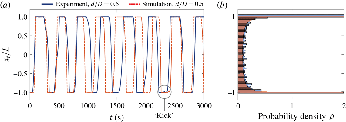
Following the numerical methods in Bernardin (Reference Bernardin2003), (2.4) can be integrated, and one example trajectory for
 $d/D=0.5$
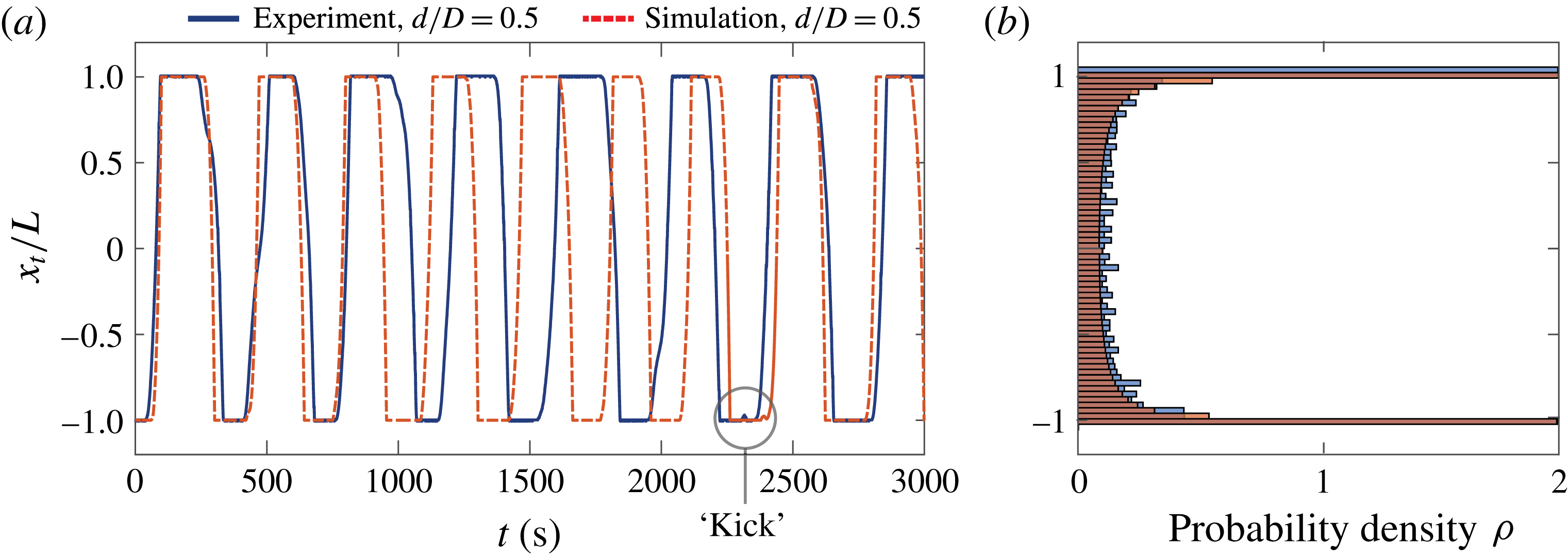
is shown in figure 4(a). Comparing to the experiment, the simulation captures the same dynamics as well as stochastic behaviours. As indicated in figure 4(a), a ‘kick’ can be spotted when the plate is about to leave the wall, and it is a consequence of the noise acting on
 $y_{t}$
. As
 $y_{t}\rightarrow x_{t}$
, the drift in
 ${\dot{x}}_{t}$
is approaching 0, so the noise could temporarily change the sign of
 ${\dot{x}}_{t}$
and give a brief push to the plate. Moreover, the probability density of
 $x_{t}$
can be computed through the statistics of integrating the SDE. Figure 4(b) shows the numerical result compared to the experiment.
Typical trajectory and histogram obtained from experiment and SVI for
 $d/D=0.5$
. (a) Trajectory extracted from experiment (blue) compared to the SDE simulation (red dashed). The SVI captures the oscillatory behaviour and shows stochastic features such as the ‘kick’ at the boundary. (b) Histogram of the plate centre
 $x_{t}/L$
. Simulation and experiment have the same colour scheme as in (a).
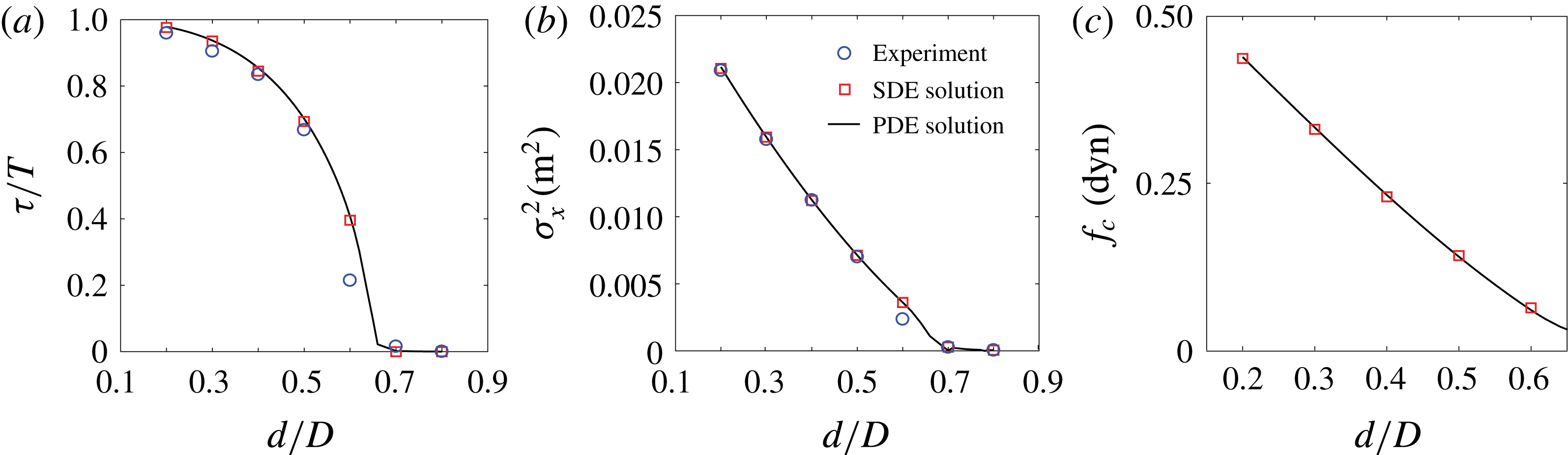
One can explore other physical quantities that are susceptible to the noise. When the probability distribution reaches its steady state, the time average of physical measurement should agree with its steady state expectation value obtained in the backward PDE, and here we can demonstrate such agreement with several examples. In figure 5, PDE quantities are obtained by finding
 $\lim _{s\rightarrow \infty }u(x,y,0)$
where
 $u$
solves (4.7) (the dependency w.r.t.
 $s$
comes from the terminal condition
 $u(x,y,s)=f(x,y)$
). Numerically (Mertz et al.
Reference Mertz, Stadler and Wylie2017), we solve the stationary version of (4.7),
 $$\begin{eqnarray}\left.\begin{array}{@{}c@{}}\displaystyle \unicode[STIX]{x1D706}u_{\unicode[STIX]{x1D706}}-Au_{\unicode[STIX]{x1D706}}=f\quad \text{in }{\mathcal{D}},\quad \unicode[STIX]{x1D706}u_{\unicode[STIX]{x1D706}}-B_{+}u_{\unicode[STIX]{x1D706}}=f\quad \text{in }{\mathcal{D}}_{+},\\ \displaystyle \quad \unicode[STIX]{x1D706}u_{\unicode[STIX]{x1D706}}-B_{-}u_{\unicode[STIX]{x1D706}}=f\quad \text{in }{\mathcal{D}}_{-},\quad \frac{\unicode[STIX]{x2202}u_{\unicode[STIX]{x1D706}}}{\unicode[STIX]{x2202}y}=0\quad \text{in }y=\pm \frac{D}{2}.\end{array}\right\}\end{eqnarray}$$
Here
 $\unicode[STIX]{x1D706}>0$
is a small parameter replacing the time. It can be shown that
 $$\begin{eqnarray}\lim _{\unicode[STIX]{x1D706}\rightarrow 0}\unicode[STIX]{x1D706}u_{\unicode[STIX]{x1D706}}(x,y)=\lim _{s\rightarrow \infty }u(x,y,0).\end{eqnarray}$$
Figure 5(a) shows the portion of time that the plate stays at the boundary, which can be obtained through setting
 $f(x,y)=\mathbf{1}_{\{|x|=L\}}$
. There is a clear trend that small plates tend to stay at the boundary longer. There appears to be a deviation at
 $d/D=0.6$
, which could be due to the fact that the plate size is close to the critical value
 $d_{c}$
. Another quantity we can measure is the steady state variance of the plate centre
 $x_{t}$
, with
 $f(x,y)=x^{2}$
in the PDE. In figure 5(b) we can see that the model captures the dynamics almost exactly, except for the criticality. The variance decreases monotonically as the plate size increases, which is a consequence of the plate spending less time on the boundary. Around the criticality, a deviation exists between experiments and the SVI model, which could be due to the fact that our SVI model is a first-order approximation to the true dynamics, and higher-order effects would appear and dominate the dynamics once the system reaches the criticality of the first-order system.
Physical quantities obtained from the SVI model compared to the measurements; all quantities are measured and computed in the steady state of statistics. (a) The portion of time that the plate stays at the boundary. Monte Carlo simulation (SDE solution) and the solution of the Kolmogorov equation (PDE solution) agree with experimental measurements. (b) Variance of the plate position can be accurately predicted by the SVI model. (c) Mean contact force computed through the SVI model, which is not yet available from experiments.
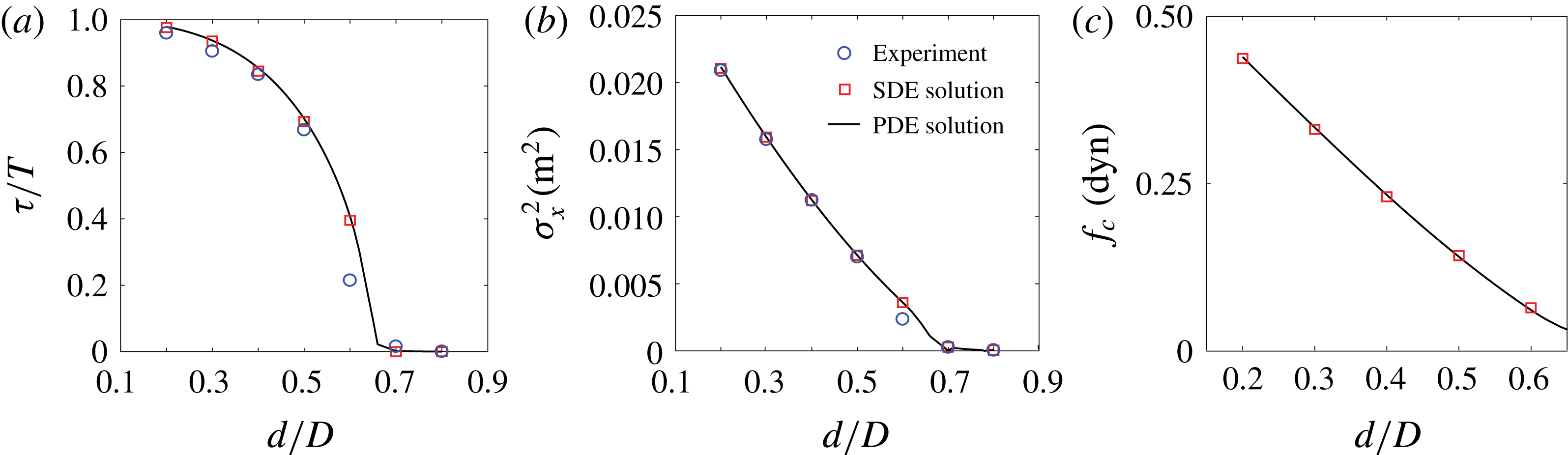
In the above examples, one has to note that the strength of noise
 $\unicode[STIX]{x1D70E}=0.001$
is estimated through the method described in § 2, which only utilizes the data from the trapped state
 $d/D=0.8$
. Hence figure 5(a,b) is further evidence of the validity of our noise modelling. Moreover, the predictions made above become far worse without the presence of noise, which is a consequence of the stochastic nature of the physics.
The SVI model can also predict quantities that would be hard or infeasible to measure experimentally. When the plate contacts the boundary, a contact force exists due to the fluid force pushing the plate into the wall. From (2.1), the net fluid force on the plate at the right boundary is
 $F(L,y_{t})=\unicode[STIX]{x1D702}w/\unicode[STIX]{x1D706}\int _{L-d/2}^{L+d/2}v_{r}\,\text{d}x=-\text{d}w\unicode[STIX]{x1D702}/\unicode[STIX]{x1D706}[\unicode[STIX]{x1D6FC}(2d)L-\unicode[STIX]{x1D6FC}(d)y_{t}]$
. Without motion, the mean contact force equals the mean fluid force, which can be expressed as
 $f_{c}=\lim _{t\rightarrow \infty }\mathbb{E}[F(x_{t},y_{t})|x_{t}=L]=-\text{d}w\unicode[STIX]{x1D702}/\unicode[STIX]{x1D706}\{\unicode[STIX]{x1D6FC}(2d)L-\unicode[STIX]{x1D6FC}(d)\lim _{t\rightarrow \infty }\mathbb{E}[y_{t}|x_{t}=L]\}$
. Figure 5(c) shows the mean contact force estimated through the simulation – the magnitude of this force is of the order of 0.5 dyne, which would be difficult to measure experimentally. In our setting, we used
 $f(x,y)=y\mathbf{1}_{\{x=L\}}$
and the formula
 $\mathbb{E}[y_{t}|x_{t}=L]=(\mathbb{E}(f(x_{t},y_{t})))/(\mathbb{P}(x_{t}=L))$
. The mean contact force has further applications in geophysics, where the contact between continents causes geological events such as mountain formation and earthquakes. Although our SVI model only provides a minimal approximation towards the lab-scale experiment, the combination of our approach and the analysis of thermal convection with non-trivial boundary conditions (for example, Bakhuis et al.
Reference Bakhuis, Ostilla-Mnico, van der Poel, Verzicco and Lohse2018) could be adopted to future modelling of geodynamics.
In conclusion, SVIs have been identified as a mathematical framework to model the solid–fluid interactions in thermal convection. In particular, we have noticed that a stochastic version of the ZZ model is well-posed in the framework of a SVI. In contrast to the deterministic model, it is not straightforward to formulate the stochastic problem as a well-posed piecewise dynamics, which is due to the mathematical subtleties inherent to the white noise. SVI theory leads to a solid framework for Kolmogorov equations of the stochastic ZZ model. This allows us to employ the machinery of Markovian tools and thus Kolmogorov equations, and apply them to the modelling of fluid problems. Here we have derived the corresponding Kolmogorov equations and used them for the numerical study of the stochastic ZZ model. From a numerical perspective, techniques based on PDEs are more efficient than Monte Carlo methods for a low-dimensional state variable (dimension
 ${\leqslant}3$
).
In coming papers, we plan to investigate several issues such as the property of long-term behaviour and metastable states, applications towards other fluid–structure interaction problems, among others.
Acknowledgements
We thank NSFC grant 11572230, 1161101053, 11601335, 11472106 and NSF grant 1805506, DMS-1463062 for supporting this project.