


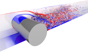





1. Introduction
Although problems involving symmetric geometries do exhibit symmetric properties at lower Reynolds numbers, for sufficiently large Reynolds numbers it has been shown that such flows can transition to an asymmetric state. These types of flow transitions have been observed for flows in symmetric expanding channels (Durst, Melling & Whitelaw Reference Durst, Melling and Whitelaw1974; Cherdron, Durst & Whitelaw Reference Cherdron, Durst and Whitelaw1978), dual parallel jets in a channel (Goodwin & Schowalter Reference Goodwin and Schowalter1996; Soong, Tzeng & Hsieh Reference Soong, Tzeng and Hsieh1998), channels with sudden contractions (Chiang, Sau & Hwang Reference Chiang, Sau and Hwang2011) and flows in constricted channels (Pitt, Sherwin & Theofilis Reference Pitt, Sherwin and Theofilis2005). To investigate the nature of these flow transitions, studies conducted by Fearn, Mullin & Cliffe (Reference Fearn, Mullin and Cliffe1990) and Shapira, Degani & Weihs (Reference Shapira, Degani and Weihs1990) for the symmetric channel expansion, Goodwin & Schowalter (Reference Goodwin and Schowalter1996) for the dual parallel jets in a channel, and Chiang et al. (Reference Chiang, Sau and Hwang2011) for the channel constriction, have shown that these transitions to asymmetric states are the results of symmetry-breaking bifurcations in the Navier–Stokes equations. As the Reynolds number is further increased, three-dimensional effects become increasingly important. Chiang et al. (Reference Chiang, Sheu, Hwang and Sau2001) were able to show that for channels with sufficiently large spanwise extents, there is a breaking of the translational symmetry along the span, resulting in different orientations of the asymmetric flow on each side of the domain. It was also determined this mode coexisted with a purely asymmetric mode. With even further increases to the Reynolds number, the flow eventually becomes turbulent, and within this regime, investigations have been conducted for the symmetric expanding channel (Escudier, Oliveira & Poole Reference Escudier, Oliveira and Poole2002; Duwig, Salewski & Fuchs Reference Duwig, Salewski and Fuchs2008; Casarsa & Giannattasio Reference Casarsa and Giannattasio2008) and the flow through an obstructed channel (El Khoury et al. Reference El Khoury, Pettersen, Andersson and Barri2010), which have also reported asymmetries in the mean flow.
A similar flow configuration that has garnered interest recently is the flow past a bluff body confined in a channel, due to its relevance in flows past heat exchangers and flows past buildings within cities. For sufficiently small blockages, the flow has been shown to retain its symmetry (Rehimi et al. Reference Rehimi, Aloui, Nasrallah, Doubliez and Legrand2008; Kanaris, Grigoriadis & Kassinos Reference Kanaris, Grigoriadis and Kassinos2011). However, as the confining walls are brought closer to the cylinder, Sahin & Owens (Reference Sahin and Owens2004), Ooi et al. (Reference Ooi, Chan, Aljubaili, Mamon, Leontini, Skvortsov, Mathupriya and Hasini2020) and Aljubaili et al. (Reference Aljubaili, Chan, Lu and Ooi2022) found that the two-dimensional flows past circular cylinders and flat plates, normal to the flow direction, exhibit asymmetric properties. For both cases, linear stability analyses showed that the emergence of these asymmetric flow regimes was the result of a pitchfork bifurcation from a symmetric state. For the case of the circular cylinder, Ooi et al. (Reference Ooi, Chan, Aljubaili, Mamon, Leontini, Skvortsov, Mathupriya and Hasini2020) performed additional two-dimensional simulations for a blockage ratio of  $\beta =0.7$, where the blockage ratio is defined as the ratio between the cylinder diameter to the channel height and found that the resulting asymmetric wake remained steady up to a Reynolds number of
 ${\textit {Re}}=500$. Extending the analysis of a confined circular cylinder to Reynolds numbers of
 ${\textit {Re}}=3900$, Ooi et al. (Reference Ooi, Lu, Chan, Cao, Leontini and Skvortsov2022) performed three-dimensional direct numerical simulations (DNS) for various blockage ratios up to
 $\beta =0.7$. It was found that for a blockage ratio of
 $\beta =0.7$ the wake was asymmetric in the mean sense for at least
 $500$ dimensionless time units, with no preference for either side of the channel.
The results of previous investigators have shown that under large enough blockage and Reynolds numbers, the mean flow past a confined bluff body is asymmetric. However, based on the observations of Chiang et al. (Reference Chiang, Sheu, Hwang and Sau2001), it appears the asymmetries in confined flows can flip their orientation along the span for sufficiently large spanwise domains. To the best of the authors’ knowledge, such a flipping phenomena has not been observed previously in the flow past a confined bluff body. In this study, our primary aim is to investigate whether such a spanwise flipping phenomena occurs for flows past confined circular cylinders. If such a phenomena occurs, how does it modify the flow compared with the smaller spanwise domains considered by previous investigators. To do so, we conduct three-dimensional simulations for a range of Reynolds numbers for spanwise domains up to  $20$ times the cylinder diameter.
2. Methodology
2.1. Problem set-up
We consider the problem of a circular cylinder with diameter  $D$ placed symmetrically in a channel of height
 $H$ as shown in figure 1. Upstream of the cylinder, it was assumed the flow to be laminar and fully developed, with a streamwise velocity profile given by
 \begin{equation} u(y)=U\left[1-\left(\frac{2y}{H}\right)^{2}\right], \end{equation}
where  $U$ is the centreline velocity at the inlet and
 $y$ is the wall-normal coordinate. We also define the blockage ratio as the ratio of the cylinder diameter and the channel
 $\beta =D/H$, which we have fixed at
 $\beta =0.7$, and the Reynolds number as
 ${\textit {Re}}=UD/\nu$,
 $\nu$ is the kinematic viscosity of the fluid. The non-dimensionalisation arises from viewing the problem as a confined wake flow and therefore following the scaling typical to unconfined bluff body flows (Dong et al. Reference Dong, Karniadakis, Ekmekci and Rockwell2006; Parnaudeau et al. Reference Parnaudeau, Carlier, Heitz and Lamballais2008). The problem may also be viewed as a blocked channel flow, where one would consider the channel height
 $H$ as a length scale. Ooi et al. (Reference Ooi, Lu, Chan, Cao, Leontini and Skvortsov2022) showed that under such scaling, the channel centreline Reynolds number
 ${\textit {Re}}_{cl}=UH/(2\nu )$ is related to
 ${\textit {Re}}$ by a constant
 $1/(2\beta )$.
Schematic diagram of the geometry considered, where  $L_i$ is the inlet length,
 $L_o$ is the outlet length,
 $D$ is the cylinder diameter and
 $H$ is the channel height.

2.2. Numerical method
DNS of the three-dimensional incompressible Navier–Stokes equations were carried out using the CPU-based spectral element solver Nek5000 (Fischer, Lottes & Kerkemeier Reference Fischer, Lottes and Kerkemeier2008) and its GPU equivalent NekRS (Fischer et al. Reference Fischer2022). The method involves the discretisation of the domain into  $E$ hexahedral macro-elements, where the solution is expanded using a tensor product of
 $N$th-order polynomials defined by the values at the Gauss–Lobatto–Legendre (GLL) nodes of the same order.
To discretise our domain, we consider a variety of meshes with a similar topology to that shown in figure 2, with descriptive statistics given in table 1. Here,  $E_{cyl}$,
 $E_{xy}$,
 $E_{z}$ and
 $E_{elem}$ are the number of macro-elements along the azimuthal direction, in the
 $xy$-plane, along the spanwise direction, and in total. As for the boundaries, a Dirichlet boundary condition given by (2.1) was applied for the inlet, no-slip boundary conditions were applied to the channel walls and the cylinder surface, periodicity was assumed along the spanwise boundaries and the stabilised outlet boundary condition by Dong, Karniadakis & Chryssostomidis (Reference Dong, Karniadakis and Chryssostomidis2014) was applied to the outlet.
Topology of the macro-element mesh used in the  $S5$ case.

Summary of cases considered in this study with mesh statistics.

To ensure that the meshes are accurately resolving the flow, we compute the ratio of the length scale of each micro-element  $\varDelta =V_{m}^{1/3}$, where
 $V_{m}$ is the volume of the micro-element, to the Kolmogorov length scale
 $\eta =(\nu ^{3}/\varepsilon )^{1/4}$. Here
 $\varepsilon$ is computed based on the instantaneous dissipation
 \begin{equation} \varepsilon=\nu\left(\frac{\partial u^{\prime}_{i}}{\partial x_{j}}\frac{\partial u^{\prime}_{i}}{\partial x_{j}}\right), \end{equation}
where the primed quantities denote the fluctuating fields  $u_{i}^{\prime }=u_{i}-\bar {u}_{i}$, with the overbar indicating a time-averaged field. We believe this gives a more conservative result than the mean dissipation commonly used in the literature as it is capable of capturing highly turbulent bursts that may be smoothed out in an averaging process. Instantaneous snapshots of the dissipation and, hence, Kolmogorov length scale were computed using the time-averaged flow for
 $\bar {u}_{i}$ and instantaneous realisations of the flow at different times for
 $u_{i}$. We plot in figure 3 representative slices of
 $\varDelta /\eta$ for the cases
 $S1$,
 $S4$ and
 $S5$. For
 ${\textit {Re}}=300$
 $(S1)$, we find
 $\varDelta /\eta$ to be relatively small across the near-wake region
 $x/D<10$. In this case, the maximal value did not exceed
 $4$ during the simulation. At Reynolds number,
 ${\textit {Re}}=1000$
 $(S4)$, the range of
 $\varDelta /\eta$ observed fell between
 $0\leq \varDelta /\eta \leq 7.5$. These results satisfy the criteria set forth by Moin & Mahesh (Reference Moin and Mahesh1998), which for DNS, finds grid spacing of
 $O(\eta )$ sufficient. Finally, for the highest-Reynolds-number case considered
 ${\textit {Re}}=3900$, figure 3(c) shows that
 $\varDelta /\eta$ is predominantly less than
 $7.5$ for the majority of the near-wake region, with small turbulent bursts resulting in
 $\varDelta /\eta$ locally increasing to approximately
 $17$. It is of note
 $S5$ is based on the same two-dimensional mesh as used by Ooi et al. (Reference Ooi, Lu, Chan, Cao, Leontini and Skvortsov2022) for the same
 ${\textit {Re}}$, where it was found sufficient for DNS. To also ensure that the near-wall dynamics are well resolved, it is typical in wall-bounded flows to compare the height of the first grid point
 $\Delta y_{1}$ with the viscous length scale
 $\nu /u_{\tau }$, where
 $u_{\tau }=\sqrt {\tau _{w}/\rho }$ is the friction velocity, with
 $\tau _{w}$ being the shear stress at the wall, and
 $\rho$ the fluid density (Zahtila et al. Reference Zahtila, Lu, Chan and Ooi2023). We therefore plot in figure 4 the distribution of
 $y^+=\Delta y_{1}u_{\tau }/\nu$ values along the cylinder surface along with the channel walls for different Reynolds numbers. We see in all cases that
 $y^+$ is less than unity along the cylinder surface and the channel walls, indicating that the computational meshes are capable of resolving the boundary layers.
Contours of the ratio  $\varDelta /\eta$ for (a)
 ${\textit {Re}}=300$, (b)
 ${\textit {Re}}=1000$ and (c)
 ${\textit {Re}}=3900$.

Distribution of  $y^+$ values of the first grid point for (a) the cylinder surface and (b) the channel walls. The blue, grey and red lines denote the
 $y^+$ values for
 ${\textit {Re}}=300$,
 $1000$ and
 $3900$, respectively. In (b), dotted and dashed lines denote the top and bottom walls, respectively.

Nonetheless, the aim of this work being observation of large-scale features in confined cylinder flows, we believe that although case  $S5$ is marginally or slightly under resolved, it does capture and highlight the presence of these large structures.
2.3. Code validation
To validate the performance of NekRS, we consider the case of uniform flow past an unconfined circular cylinder at Reynolds number of  $Re=3900$, which has been studied extensively both numerically and experimentally. A recent review is given in the work of Jiang & Cheng (Reference Jiang and Cheng2021). To approximate such a flow configuration, we consider a mesh with blockage ratio of
 $\beta =0.025$, which amounts to the crossflow domain of
 $y/D\in [-20,20]$ as well as inlet and outlet lengths of
 $L_{i}/D=10$ and
 $L_{o}/D=30$. For this case, we used a uniform Dirichlet inlet boundary condition of
 $(u,v,w)=(U,0,0)$ and symmetry boundary conditions for the domain top and bottom.
For this simulation, we solve the Navier–Stokes equations with an initial condition of zero fluid velocity throughout the entire domain. The simulations were then run for some period  $t_{0}$ until the flow reached a statistically stationary state, which in this case takes approximately
 $t_{0}U/D=250$. From this point, statistics were collected over an additional
 $500D/U$. Results of the velocity fluctuations at different streamwise locations are shown in figure 5. We find that the data agrees well with the experimental results of Parnaudeau et al. (Reference Parnaudeau, Carlier, Heitz and Lamballais2008) and the large eddy simulations of Jiang & Cheng (Reference Jiang and Cheng2021), providing confidence the code is capable of accurately simulating bluff body flows.
Time- and spanwise-averaged profiles of the (a) streamwise and (b) crossflow velocity fluctuations at the streamwise locations  $x/D=1.06$,
 $1.54$ and
 $2.02$ for the unconfined case at
 ${\textit {Re}}=3900$. (——) Present DNS,
 $(\bullet )$ experimental data of Parnaudeau et al. (Reference Parnaudeau, Carlier, Heitz and Lamballais2008), (– – –) large eddy simulation data of Jiang & Cheng (Reference Jiang and Cheng2021) (Case 6).

3. Results
3.1. Instantaneous flow structures
To understand the spanwise effects on the flow, we first present visualisations of the instantaneous flow for the largest domain size of  $L_{z}/D=20$ using the
 $\lambda _{2}$ vortex identification criterion of Jeong & Hussain (Reference Jeong and Hussain1995). In this method we compute the eigenvalues of symmetric tensor
 $\boldsymbol {S}^{2}+\boldsymbol {\varOmega }^{2}$, where
 $\boldsymbol {S}$ and
 $\boldsymbol {\varOmega }$ are the symmetric and antisymmetric components of the velocity gradient tensor. Isosurfaces of the second eigenvalue
 $\lambda _{2}$ are then plotted which may be used to identify vortical structures. For the simulation at
 ${\textit {Re}}=300$, the flow was initialised with an initial condition of zero velocity everywhere, whereas for
 ${\textit {Re}}=1000$ and
 $3900$, the flow was restarted from a fully developed flow at
 ${\textit {Re}}=300$. An indicative realisation of the flow was then taken after a period of at least
 $100D/U$.
We begin by looking at a Reynolds number of  ${\textit {Re}}=300$ in figure 6, wherein isosurfaces are taken for
 $\lambda _{2}=-0.5$. The primary observed feature evident in the cylinder wake is shedding of long spanwise vortices across the domain. We also observe that thin streamwise vortices form at some locations along the span, and at other locations, we primarily see the formation of spanwise rollers. To understand the behaviour along these locations, we plot in figure 7 visualisations of the instantaneous spanwise vorticity
 $\omega _{z}$ along the spanwise planes
 $z/D=2$,
 $4$,
 $8$ and
 $14.5$, and in figure 8 the same contours overlain with isosurfaces of
 $\lambda _{2}=-0.5$ colourised by the spanwise vorticity. We first take a closer look at flow along the spanwise plane
 $z/D=4$, where streamwise vortices are present. Figure 7(b) shows that the separated cylinder shear layers (CSLs) roll up to form spanwise vortices. As the vortex grows, it eventually gets cut off by the formation of a spanwise vortex from the opposing CSL, resulting in vortices being shed in an alternating manner. Such a pattern is characteristic of von Kármán shedding (see, e.g., Williamson Reference Williamson1996). These vortices are then convected downstream and cross the centreplane
 $y/D=0$, where they merge with the shed vortices from the opposing wall, giving rise to a reverse von Kármán wake (Zovatto & Pedrizzetti Reference Zovatto and Pedrizzetti2001). The flow structures given in figure 8(b) also show that along with the spanwise vortices, the streamwise vortices observed previously in figure 6 are curved towards the centre of the channel due to the reverse von Kármán wake (Camarri & Giannetti Reference Camarri and Giannetti2010). These fine-scale streamwise vortices have a wavelength of approximately
 $D$, which is similar to that reported by Barkley & Henderson (Reference Barkley and Henderson1996) and Camarri & Giannetti (Reference Camarri and Giannetti2010) for a mode B instability at
 $\beta =0$ and
 $\beta =0.2$, respectively. However, the linear stability results of Griffith et al. (Reference Griffith, Leontini, Thompson and Hourigan2011) and Ooi et al. (Reference Ooi, Chan, Aljubaili, Mamon, Leontini, Skvortsov, Mathupriya and Hasini2020) only determine the existence of a mode which shared the same symmetries as mode A for
 $\beta =0.5$. In the present case, the chaotic nature of the flow makes it unclear whether the flow shares the same symmetries as the mode B instability in the lower blockage cases.
Isosurfaces of  $\lambda _{2}=-0.5$ for
 ${\textit {Re}}=300$ colourised by the streamwise vorticity. Regions dominated by packets of coherent: (i) streamwise vortices demarcated by the solid ellipse; and (ii) spanwise vortices by the dotted ellipse.

Contours of the spanwise vorticity along several spanwise planes (a)  $z/D=2$, (b)
 $z/D=4$, (c)
 $z/D=8$ and (d)
 $z/D=14.5$ for
 ${\textit {Re}}=300$. The orange dots indicate the locations of the probes used to construct the spectra and spacetime diagram for this flow configuration.

Contours of the spanwise vorticity for  ${\textit {Re}}=300$ as in figure 7. Overlain are isosurfaces of
 $\lambda _{2}=-0.5$ between (a)
 $2\leq z/D\leq 3$, (b)
 $4\leq z/D\leq 5$, (c)
 $8\leq z/D\leq 9$ and (d)
 $14.5\leq z/D\leq 15.5$. Isosurfaces are colourised by the spanwise vorticity.

Looking now at the flow along the spanwise plane  $z/D=2$, where streamwise rib-like vortex structures are no longer evident in figure 6, figure 7(a) shows a very different structure at the tail of the wake. Unlike with the previous case at
 $z/D=4$, there is a distinct lack of any roll up of the CSL, resulting in a local suppression of the formation of von Kármán vortices. Although for the sake of brevity, we refer to this phenomena as wake suppression hereinafter. In this case, the shear layers off the top and bottom of the cylinder combine near the centreline, which we refer to herein as the tail of the wake. Downstream of this point, we see that the separated wall shear layer (WSL) becomes unstable via a Kelvin–Helmholtz-type instability resulting in the spanwise vortices observed in figure 8. Comparison of the tail of the wake with the two-dimensional simulations by Sahin & Owens (Reference Sahin and Owens2004) and Ooi et al. (Reference Ooi, Chan, Aljubaili, Mamon, Leontini, Skvortsov, Mathupriya and Hasini2020) show that the attachment of the CSLs is remarkably similar. Therefore, the local suppression of von Kármán shedding appears to be caused by the same confinement effect as the two-dimensional case. It is surprising that three-dimensionality of the flow permits both effects to occur simultaneously along different points along the span. Turning attention to additional spanwise planes
 $z/D=8$ and
 $14.5$ in figure 7(c,d), where von Kármán shedding is suppressed, we find that the tail of the wake is deflected towards the top and bottom of the channel, respectively. We refer to this instantaneous behaviour in the wake as a bias of the flow. Qualitative comparison of the flow with the two-dimensional case presented in Ooi et al. (Reference Ooi, Chan, Aljubaili, Mamon, Leontini, Skvortsov, Mathupriya and Hasini2020) shows that the wake has a similar structure. Downstream of the tail, the flow again becomes unstable forming strong spanwise vortices which may be observed in figure 8(c,d). Figures 6 and 8(c,d) also show that the formation of streamwise vortices between the spanwise rollers as the flow becomes three-dimensional.
Moving up to a higher Reynolds number of  ${\textit {Re}}=1000$, we plot isosurfaces of
 $\lambda _{2}=-10$ colourised by the streamwise vorticity in figure 9. We find that much like the previous case, there are strong spanwise vortices which appear to exist across the entire domain, along with many fine-scale streamwise vortices. To further look into the flow structures, figure 10 shows slices of the spanwise vorticity along the spanwise planes
 $z/D=13$,
 $15.5$ and
 $18$. Similar to the
 ${\textit {Re}}=300$ case, we find in figure 10(a,c) that dependent on the spanwise coordinate, the wake can bias itself towards either the channel top or bottom. There appears to be little roll up of the CSL in the wake, with the CSLs from either side of the channel combining in a similar manner to the flow at
 ${\textit {Re}}=300$. Hence, it becomes apparent there is local suppression of von Kármán shedding. The higher Reynolds number also results in unsteadiness within the near-wake region, through formation of spanwise vortices in the WSL. The formation of the spanwise vortices in the deflected WSL is also much stronger than in the undeflected WSL. The different orientations of the wake imply there exists a point in between where the wake flips, which for the given instant appears to be
 $z/D=15.5$ as indicated by the apparent lack of bias in figure 10(b). Along this plane, we see that the CSL rolls up towards the centre of the channel unlike the biased wakes. The vortices also appear to shed in a von Kármán-like manner, with vortices cutting off the formation of additional vortices in the opposing CSL. Although the interactions with the WSL attenuate the effect quite drastically. The CSL and WSL also roll up simultaneously as observed previously by Nguyen & Lei (Reference Nguyen and Lei2021) at
 $\beta =0.6$ and is caused by the coupling of the two shear layers due to their proximity. Visualisation of the flow structures in figure 11(b) does show that the spanwise vortex formed within the CSL has a much lower coherency compared with that in the WSL. The effect has also previously been observed by Ooi et al. (Reference Ooi, Lu, Chan, Cao, Leontini and Skvortsov2022) at
 $\beta =0.5$ and
 $0.7$ and is a result of the interactions with streamwise vortices formed at the tail of the wake.
Isosurfaces of  $\lambda _{2}=-10$ for
 ${\textit {Re}}=1000$ colourised by the streamwise vorticity.

Contours of the spanwise vorticity along the spanwise planes (a)  $z/D=13$, (b)
 $z/D=15.5$ and (c)
 $z/D=18$ for
 ${\textit {Re}}=1000$. The orange dots indicate the locations of the probes used to construct the spectra and spacetime diagram for this flow configuration.

Contours of the spanwise vorticity for  ${\textit {Re}}=1000$ as in figure 10. Overlain are isosurfaces of
 $\lambda _{2}=-10$ between (a)
 $13\leq z/D\leq 14$, (b)
 $15.5\leq z/D\leq 16.5$ and (c)
 $18\leq z/D\leq 19$. Isosurfaces are colourised by the spanwise vorticity.

Increasing the Reynolds number to  ${\textit {Re}}=3900$, we plot in figure 12 slices of the spanwise vorticity along three different spanwise planes,
 $z/D=9.5$,
 $12$ and
 $14.5$. Here we find that the flow strongly resembles that of the
 ${\textit {Re}}=1000$ case, with a wake that is biased towards either the top or bottom of the channel depending on the spanwise location, with the wake flipping its bias at
 $z/D=12$. Figure 13 also shows the formation of spanwise vortices due to a Kelvin–Helmholtz-type instability in the CSL and the WSL, which was also observed by Ooi et al. (Reference Ooi, Lu, Chan, Cao, Leontini and Skvortsov2022) for a smaller spanwise domain of
 $L_{z}/D={\rm \pi}$. Such a phenomenon has also been observed in unconfined bluff body flows at similar Reynolds number (Williamson Reference Williamson1996; Dong et al. Reference Dong, Karniadakis, Ekmekci and Rockwell2006). We also find that the breakdown of the shear layers again appears to be strongly coupled to their interaction, with the formation of opposite signed vortices in a pairwise manner. In figure 13, compared with the
 ${\textit {Re}}=1000$ case, the vortex within the CSL appears to be much more distinct, possibly due to the earlier breakdown of the shear layers. We also see that the length of the wake decreases from approximately
 $4D$ to
 $2D$. Decreases in the wake length have previously been documented for unconfined cylinder flows and is associated with the formation of Kelvin–Helmholtz vortices in the shear layer (e.g. Unal & Rockwell Reference Unal and Rockwell1988; Williamson Reference Williamson1996). A similar effect is responsible for the decrease in the wake length in this case as well. Further, the asymmetric wake appears to be slightly shorter than that found in Ooi et al. (Reference Ooi, Lu, Chan, Cao, Leontini and Skvortsov2022) at approximately
 $2D$ compared with their result of
 $2.5D$. As we move downstream of the tail, figure 13 also shows the Kelvin–Helmholtz vortices rapidly break down into much finer-scale structures.
Contours of the spanwise vorticity along spanwise planes (a)  $z/D=9.5$, (b)
 $z/D=12$ and (c)
 $z/D=14.5$ for
 ${\textit {Re}}=3900$. The orange dots indicate the locations of the probes used to construct the spectra and spacetime diagram for this flow configuration.

Contours of the spanwise vorticity for the case of  ${\textit {Re}}=3900$ as in figure 12. Overlain are isosurfaces of
 $\lambda _{2}=-15$ between (a)
 $9.5\leq z/D\leq 10.5$, (b)
 $12\leq z/D\leq 13$ and (c)
 $14.5\leq z/D\leq 15.5$. Isosurfaces are colourised by the spanwise vorticity.

3.2. Near-wake spectra
To determine time scales of the phenomena featured in the previous section, we plot the spectra of the streamwise velocity for  ${\textit {Re}}=300$,
 $1000$ and
 $3900$ cases in figure 14. For each of these cases, the probe was chosen to be at a point near the tail of the wake and projected onto the centreline as shown by the orange dot in figures 7, 10 and 12, and are the same as those used in the spacetime diagrams discussed in the subsequent section. This amounted to streamwise locations of
 $x/D=3$,
 $4$ and
 $2$ for the
 ${\textit {Re}}=300$,
 $1000$ and
 $3900$ cases, respectively. Although we found there was little difference in the peak locations when moving the probe slightly upstream and downstream of the point chosen. The spectra have also been averaged in the homogeneous direction as there was no significant spanwise dependence in the results.
Streamwise velocity spectra for (a)  ${\textit {Re}}=300$ at
 $(x/D,y/D)=(3,0)$, (b)
 ${\textit {Re}}=1000$ at
 $(x/D,y/D)=(4,0)$ and (c)
 ${\textit {Re}}=3900$ at
 $(x/D,y/D)=(2,0)$. The dashed line depicts the cutoff frequency used in the filtering process.

For the lowest-Reynolds-number case studied,  ${\textit {Re}}=300$, there is a prominent peak at a frequency of
 $fD/U\approx 0.5$, which is indicative of the von Kármán shedding frequency
 $f_{VK}$. There are additional peaks at integer multiples of
 $f_{VK}$ that are associated with harmonics of the von Kármán shedding frequency. Moving up to
 ${\textit {Re}}=1000$, two separate peaks at
 $fD/U\approx 0.65$ and
 $0.9$ are present. Visualisations of the instantaneous flow in figure 10 show that one of these peaks corresponds to the formation of the spanwise vortex in the WSL, which is then convected past the probe location. The second is related to the von Kármán-like shedding along the plane with flipping bias. Finally, in figure 14(c), we see for the
 ${\textit {Re}}=3900$ case that there are two distinct peaks at
 $fD/U\approx 1.1$ and
 $2.3$, matching the peaks observed by Ooi et al. (Reference Ooi, Lu, Chan, Cao, Leontini and Skvortsov2022) for a smaller spanwise domain of
 $L_{z}/D={\rm \pi}$. The smaller peak at
 $f_{SL}D/U\approx 2.3$ was found by Ooi et al. (Reference Ooi, Lu, Chan, Cao, Leontini and Skvortsov2022) to be from the formation of Kelvin–Helmholtz vortices in the shear layer, whereas for
 $fD/U\approx 1.1$, due to the absence of von Kármán shedding, it was found the peak corresponds to the merging of vortices as the peak was close to the subharmonic frequency
 $f_{SL}/2$. Similar findings were also made by Nguyen & Lei (Reference Nguyen and Lei2021) for a slightly lower blockage of
 $\beta =0.6$. As von Kármán shedding is absent in this case as well, we argue that much like the smaller domain case of Ooi et al. (Reference Ooi, Lu, Chan, Cao, Leontini and Skvortsov2022), the lower-frequency peak is indicative of vortex merging.
3.3. Long-term behaviour
In § 3.1, the basic observation was the existence of a flow with an instantaneous bias towards one side of the channel modulated along the span, but we now focus on the temporal effects on these flow structures. To begin with, we consider the lowest-Reynolds-number case of  ${\textit {Re}}=300$, which was shown in figures 7 and 8 to locally exhibit a von Kármán wake or a suppressed wake that may be biased towards one side of the channel at different points along the span. To be able to characterise the temporal behaviour of the wake, we consider the placement of a probe near the tail of the wake where the two CSLs meet. To explain how the method will be used to capture the wake behaviour, we plot in figure 15(a) a time series of the crossflow velocity at the point
 $(x/D,y/D,z/D)=(3,0,10.0)$. The grey line here represents the raw signal, composed of time-varying low and high fluctuation states. In the intervals of low fluctuations, we do note that the signal does begin to deviate from
 $v/U=0$, which does correspond to the flow beginning to wall bias. Overlain in figure 15(a) are contours of the instantaneous spanwise vorticity at
 $(t-t_{0})U/D=200$. We see that the deflection of the bottom shear layer towards the top of the channel results in a net positive crossflow velocity at the probe location, provided it is placed within the appropriate shear layer. We also see that the local suppression of von Kármán shedding, as observed by the lack of shear layer roll up, results in minimal movement of the shear layers, hence the low fluctuations in the crossflow velocity. Moving to the periods of high fluctuations, we plot an example of the instantaneous spanwise vorticity at
 $(t-t_{0})U/D=700$ in figure 15(a). Within this flow regime, we see the formation of distinct von Kármán vortices. These vortices will induce strong alternating regions of positive and negative crossflow velocity, and when convected downstream will result in the large-amplitude fluctuations in the crossflow velocity as they cross the probe location. Moreover, due to the symmetry of the shedding process, the mean velocity within this regime is relatively close to zero.
Time-series of (a) the (light grey solid line) raw and (black solid line) low-pass filtered crossflow velocity signals and (b) (solid line) high-pass filtered crossflow velocity signal and its (dashed line) envelope for  ${\textit {Re}}=300$. The probe is placed at the streamwise location
 $x/D=3$ along the spanwise plane
 $z/D=10$. Overlain in (a) are contours of the spanwise vorticity at
 $(t-t_{0})U/D=200$ and
 $700$ along with an orange dot to indicate the location of the probe.

In order to further examine the flow, we therefore need to isolate the two wake regimes, which may be done using the following decomposition. To do so, we make the following assumption based on the observations in figure 15(a). When the wake is of von Kármán type, the periodic shedding of alternating vortices yields a relatively short time scale given by  $f_{VK}D/U=0.5$, whereas the time scale when shedding is suppressed and the wake is biased appears to be much longer. Therefore, this separation of the time scales allows us to apply a filtering process to isolate the two different wake behaviours. We therefore apply a low-pass filter with a non-dimensional cut-off frequency
 $f_{c}D/U$, which we choose to be
 $0.2$. Applying this to the crossflow velocity, which we denote
 $\tilde {v}$, at the point
 $(x/D,y/D,z/D)=(3,0,10.0)$ gives the black line in figure 15(a). We see here that the filter does not effect the signal whilst shedding is locally suppressed, as expected. However, in the von Kármán shedding regime, the oscillations have been significantly damped out, with the resulting signal slightly oscillating about
 $v/U=0$. Finally, for the von Kármán shedding regime, we plot the remainder of the signal, or, equivalently, that obtained using a high-pass filter, as the dark grey line in figure 15(b). As the shedding is characterised by large-amplitude fluctuations in the crossflow velocity, it therefore suffices to consider only the signal's amplitude profile. To do this, we apply a Hilbert transform to the data
 $v(t)$, denoted
 $\mathcal {H}(t)$, which may be used to obtain the associated analytic signal
 $Z(t)$,
 \begin{equation} Z(t)=v(t)+{\rm i}\mathcal{H}(t)=v_{A}(t){\rm e}^{{\rm i}\phi(t)}, \end{equation}
where  $v_{A}$ is the instantaneous modulus and
 $\phi (t)$ is the instantaneous phase. Then
 $v_{A}$ can be shown to represent the amplitude profile of the original signal, which is plotted as the dashed line in figure 15(b) (for additional information on the Hilbert transform, we refer the reader to Mathis, Hutchins & Marusic Reference Mathis, Hutchins and Marusic2009).
Looking now at the spanwise effect on the flow, we plot contours of the low-pass filtered signal as well as the amplitude profile in figures 16(a) and 16(b), respectively. We observe in figure 16(a) that there exist long horizontal streaks where the filtered crossflow signal is primarily red or blue and, hence, single signed over time scales of  $100D/U$. Figure 16(b) shows these regions of single-signed filtered velocity correspond to low fluctuations in the wake, which is the result of wake suppression due to wake bias. It is also evident that both blue and red streaks exist at different points along the spanwise extent of the cylinder, thus showing that the spanwise flipping observed in figures 7 and 8 persists over long time scales. At other points of the domain, where there are small blobs of positive and negative
 $\tilde {v}$ in figure 16(a), fluctuation amplitudes in figure 16(b) are relatively large, which indicates vortex shedding. Multiple wake configurations occur at different spanwise locations and times. Intermittent switching in wake behaviour has previously been observed in the flow past side-by-side circular cylinders, where the flow is bi-stable and the wake jumps between two asymmetric states (Afgan et al. Reference Afgan, Kahil, Benhamadouche and Sagaut2011). For the side-by-side cylinders, flipping is related to the gap vortices. Bi-stability has also been observed in the flow past an Ahmed body (Grandemange, Gohlke & Cadot Reference Grandemange, Gohlke and Cadot2013a,Reference Grandemange, Gohlke and Cadotb; He et al. Reference He, Minelli, Wang, Dong, Gao and Krajnović2021), with Dalla Longa, Evstafyeva & Morgans (Reference Dalla Longa, Evstafyeva and Morgans2019) proposing the switch is caused by the formation of sufficiently large hairpin vortices. In the present case, the wake demonstrates multi-stable behaviour, in which the wake locally jumps between von Kármán shedding and suppression states, which may feature bias.
Spacetime diagram of the (a) the low-pass filtered crossflow velocity, and (b) the envelope at the location  $(x/D,y/D)=(3,0)$ over the time interval
 $0\leq (t-t_{0})U/D\leq 1000$ for
 ${\textit {Re}}=300$. The dotted lines indicate the locations and time interval where local flow statistics are taken.

Moving up to Reynolds numbers of  ${\textit {Re}}=1000$ and
 $3900$, the instantaneous snapshots in figures 10–13 show an attenuation of von Kármán shedding in the higher-Reynolds-number cases. To look at the temporal behaviour of the wake, we again plot the crossflow velocity at some point along the centreline of the channel,
 $y/D=0$. This point was chosen because it intersects the deflected shear layer as shown in figure 17 and captures the vertical movement of the fluid in the deflected shear layer, located at
 $x/D=4$ and
 $2$ for
 ${\textit {Re}}=1000$ and
 $3900$, respectively, due to wake length dependency on
 ${\textit {Re}}$. We also note that in figure 17 large fluctuations in the crossflow velocity for both cases, due to formation of vortices within the shear layer. Nonetheless, the raw crossflow signals show that generally the signal is single signed due to the deflection of the shear layer. Therefore, to isolate this, we again apply a low-pass filter with non-dimensional cutoff frequencies of
 $f_{c}D/U=0.5$ and
 $0.8$ for
 ${\textit {Re}}=1000$ and
 $3900$, respectively, based on the spectral peaks in figure 14.
Time series of the (light grey solid line) raw and (black solid line) low-pass filtered velocity signal for (a)  ${\textit {Re}}=1000$ at the streamwise location
 $x/D=4$ along the spanwise plane
 $z/D=2.9$ and (b)
 ${\textit {Re}}=3900$ at the streamwise location
 $x/D=2$ along the spanwise plane
 $z/D=17.96$. Inset are contours of the spanwise vorticity at
 $(a)$
 $(t-t_{0})U/D=100$ and
 $600$ and (b)
 $(t-t_{0})U/D=75$ and
 $400$ along with an orange dot to indicate the location of the probe.

Beginning with the flow at  ${\textit {Re}}=1000$, we conducted simulations with spanwise domains of
 $L_{z}/D=4.5$, 12 and 20. These were restarted from a fully developed flow at
 ${\textit {Re}}=300$ and allowed to run for at least
 $250D/U$ before statistics were taken. The spacetime diagram of the filtered crossflow velocity along the centreline at the streamwise location
 $x/D=4$ is given in figure 18. Here we see for the smallest spanwise domain of
 $L_{z}/D=4.5$ the predominant structure in figure 18(a) shows negative velocity indicating that the wake is biased towards the bottom of the domain. Interestingly, the spacetime diagram does not depict a consistent negative velocity throughout the spanwise direction. Visualisations of the instantaneous flow field show the length of the wake slightly varies along the spanwise direction. As a result, turbulent structures within the corresponding recirculation region make up the spotty structures highlighted by the dashed rectangle in figure 18(a). For the larger spanwise domains of
 $L_{z}/D=12$ and
 $20$, figure 18(b,c) shows the existence of alternating horizontal bands of predominantly single-signed velocity, indicating that the wake alternates between top and bottom bias along the spanwise direction. Figure 18 suggests the wavelength of these structures is quite long. As there are
 $2$ and
 $4$ streaks for
 $L_{z}/D=12$ and
 $20$, respectively, the wavelengths of these structures appears to be
 $O(10D)$. Consistent with the
 $L_{z}/D=4.5$ case, these flow configurations remain stable over long time intervals of at least
 $1000D/U$, which agrees with the results of Ooi et al. (Reference Ooi, Lu, Chan, Cao, Leontini and Skvortsov2022). Although, there is a tendency for these structures to translate along the spanwise direction, consistent with
 ${\textit {Re}}=300$.
Spacetime diagram of the low-pass filtered crossflow velocity for (a)  $L_{z}/D=4.5$, (b)
 $L_{z}/D=12$ and (c)
 $L_{z}/D=20$ at the location
 $(x/D,y/D)=(4,0)$ over the time interval
 $0\leq (t-t_{0})U/D\leq 1000$ for
 ${\textit {Re}}=1000$. The dashed rectangle is indicative of regions of variations in wake length. The dotted lines indicate the locations and time interval where local flow statistics are taken.

Next, we extend the Reynolds number up to  ${\textit {Re}}=3900$. A spanwise domain length of
 $L_{z}/D=20$ was again used and the simulation procedure gradually increased the
 ${\textit {Re}}$ number from
 ${\textit {Re}}=300$ to
 $3900$, before being run for an additional
 $100D/U$. The flow was then run for
 $500D/U$ to collect statistics, and the spacetime diagram is given in figure 19. Figure 19 shows that, consistent with the
 ${\textit {Re}}=1000$ results, there exists a flipping of the bias in the wake along the spanwise direction, with the formation of two structures with wavelengths
 $\lambda /D\approx 10$. The results also show that the structures exist for time scales of at least
 $500D/U$, with little movement along the spanwise direction but the structure size changes over time. Over the interval
 $0\leq (t-t_{0})U/D\leq 200$, we find little change in the size of large scale structures, whereas for
 $200\leq (t-t_{0})U/D\leq 500$, the negatively signed structure along the top periodic boundary shrinks in size.
Spacetime diagram of the low-pass filtered crossflow velocity at the location  $(x/D,y/D)=(2,0)$ over the time interval
 $0\leq (t-t_{0})U/D\leq 500$ for
 ${\textit {Re}}=3900$. The dotted lines indicate the locations and time interval where local flow statistics are taken.

The results at the higher Reynolds numbers of  ${\textit {Re}}=1000$ and
 $3900$ show the locally suppressed wake mode has become dominant. However, as observed in figure 17 along a constant spanwise plane, the bias in the wake can flip between the channel sides, with a time scale of
 $O(100D/U)$. We relate this finding to the flip-flopping wakes observed in flow past two side-by-side circular cylinders, where the bias flips between two orientations with a time scale orders of magnitude larger than the vortex shedding period (Afgan et al. Reference Afgan, Kahil, Benhamadouche and Sagaut2011). Here though, figures 18 and 19 show alternating horizontal regions of opposite signed
 $\tilde {v}/U$, indicating the bias flips along the spanwise direction. Therefore, the meandering of these alternating horizontal streaks in figures 18 and 19 shows that the bias in the wake moves along the span of the cylinder over time. As such, along a constant spanwise plane, the observed flip-flopping is a consequence of the movement of these large-scale structures.
The results presented in this section for  ${\textit {Re}}=1000$ indicate the observed long-term structures have a strong dependence on the spanwise domain length. With a flipping in the bias only observed for spanwise domains greater than or equal to
 $L_{z}/D=12$. Hence, we investigate whether this spanwise modulation has an intrinsic length scale. For these simulations, we restrict ourselves to the case of
 ${\textit {Re}}=1000$. Figure 18 demonstrates significant variation between domains with
 $L_{z}/D=4.5$ and
 $12$, which is the minimal spanwise domain requirement for modulating structures to first appear. To ensure there is no dependence on the initial conditions, we perform an additional test where an instantaneous snapshot of the modulated flow taken from the
 $L_{z}/D=12$ simulation domain was spatially rescaled to
 $L_{z}/D=4.5$ and used as an initial condition. The spacetime diagram of filtered crossflow velocity is given in figure 20, and shows the wake reverting to a purely bottom biased flow after
 $50D/U$. Comparison of time- and spanwise-averaged flow statistics in Appendix A also show that there is no difference with the case presented in figure 18(a). Hence, the minimal spanwise domain to observe the appearance of spanwise flipping lies between
 $L_{z}/D=4.5$ to
 $12$. Further refinement of
 $L_{z}/D$ is outside of the scope of the study, but may be of interest to researchers in future work. Moreover, based on the observations in figure 19 and the results of Ooi et al. (Reference Ooi, Lu, Chan, Cao, Leontini and Skvortsov2022), it is conceivable that similar results hold for higher Reynolds numbers as well.
Spacetime diagram of the low-pass filtered crossflow velocity at  $(x/D,y/D)=(4,0)$ for
 ${\textit {Re}}=1000$ over the time interval
 $0\leq (t-t_{0})U/D\leq 1000$ with
 $L_{z}/D=4.5$, where
 $t_{0}$ is taken at the beginning of the simulation. Here the initial condition is taken as a rescaled solution from simulations conducted with
 $L_{z}/D=12$.

The preceding domain analysis naturally stimulates questions on the sensitivity of wake physics to initial conditions. Aljubaili et al. (Reference Aljubaili, Chan, Lu and Ooi2022) and Ooi et al. (Reference Ooi, Lu, Chan, Cao, Leontini and Skvortsov2022) found a flipped the numerical solution ( $y\mapsto -y$ and
 $v\mapsto -v$) remained stable, attributed to reflectional invariance of the problem. In this study, for domain size
 $L_{z}/D=4.5$ simulations, different initial conditions confirmed existence of two asymmetric states. However, our primary focus remains in persistence of the biasing phenomena for larger spanwise domains where the wake is modulated along the span. To investigate this, we conduct simulations with
 $L_{z}/D=20$ and the following initial conditions:
(i) a flow with an initial condition of zero everywhere;
(ii) an artificially constructed asymmetric solution obtained by repeating a simulation conducted with a spanwise domain of
 $L_{z}/D=2$.

Figure 21 presents the spacetime diagrams of the filtered crossflow velocity for both sets of initial conditions. Immediately, for the solution with quiescent initial conditions, we note a single red and blue band with widths that vary between  $6D$ and
 $12D$, corresponding to positive and negative crossflow velocities, respectively. The situation is remarkably different from the case in figure 18(c), where we see two alternating bands of approximately the same width. As for the case initialised from a purely asymmetric solution, the spacetime diagram shows that the crossflow velocity is predominantly negative across the entire spanwise domain, which is expected given that the artificially generated flow had a bias towards the bottom of the channel. From figure 21, we also see that the structures do persist over long time intervals of
 $1000D/U$.
Spacetime diagram of the low-pass filtered crossflow velocity at  ${\textit {Re}}=1000$ with
 $f_{c}D/U=0.5$ for (a) case (i), quiescent initialisation and (b) case (ii), artificial repetition. The probe is placed at
 $(x/D,y/D)=(4,0)$.

3.4. Global asymmetries of the wake
The previous section highlighted the existence of solutions that displayed bias across the entire domain, along with wakes of alternating bias along the spanwise direction of the cylinder. As these biases in the wake persist over long time scales, we adopt a definition of asymmetry in the ‘mean’ sense. Specifically, we define a flow as:
(i) globally asymmetric if the time- and spanwise-averaged flow displays an asymmetry; and
(ii) locally asymmetric if there exists a spanwise location where the time-averaged flow displays an asymmetry.
Therefore, we first consider in figure 22 the time and spanwise average of the flow. Figure 22(a) shows that for  ${\textit {Re}}=300$, the time- and spanwise-averaged flow is symmetric. The global symmetry in the flow is caused by the intermittent wake switching between a locally suppressed state and a von Kármán shedding state, along with the meandering of the flow along the spanwise direction of the cylinder. As we move up to
 ${\textit {Re}}=1000$, we plot in figure 22(b) the time- and spanwise-averaged flows for each of the spanwise domains considered. We see for
 $L_{z}/D=4.5$ a global asymmetry towards the channel bottom, which is a result of the uniform orientation of the bias observed in figure 18(a), whereas for
 $L_{z}/D=12$ and
 $20$, the wakes are globally symmetric. The effect is due to the flipping in the wake bias along the span of the cylinder, which cancels out while spanwise averaging. Such a method is therefore not sensitive enough to capture the local asymmetries in the wake. We also remark the dependence on the initial conditions for larger spanwise domains does enable for both globally symmetric and asymmetric flows to exist, with analysis of the time- and spanwise-averaged flow given in Appendix A. Finally, for
 ${\textit {Re}}=3900$, figure 22
 $(c)$ shows the flow is globally symmetric despite changes in size of the horizontal streaks in figure 19. Comparisons of the flow profiles for different averaging intervals in Appendix B show that the difference between the solutions for an averaging interval of
 $200D/U$ and
 $500D/U$ are approximately 5 %. The differences are not accounted for by averaging interval, rather slight variations in the size of modulated structures observed in figure 19.
Contours of the time- and spanwise-averaged streamwise velocity for (a)  ${\textit {Re}}=300$, (b)
 ${\textit {Re}}=1000$ for spanwise domains of (b i)
 $L_{z}/D=4.5$, (b ii)
 $L_{z}/D=12$ and (b iii)
 $L_{z}/D=20$ and (c)
 ${\textit {Re}}=3900$.

3.5. Local asymmetries in the wake
In the previous section, we observed the existence of wakes which demonstrate global asymmetries, resulting from a uniform bias in the wake. We also found wakes which demonstrated a spanwise dependence on the bias were globally symmetric, due to the asymmetries cancelling out in the spanwise-averaging process. We now turn our focus into more deeply interrogating the local properties of the biases. Furthermore, for  ${\textit {Re}}=1000$, we also restrict our attention to the largest spanwise domain of
 $L_{z}/D=20$ initialised with a fully developed realisation of the flow at
 ${\textit {Re}}=300$. For additional analysis of the effect of the initial conditions, we refer the reader to Appendix A.
3.5.1. Fourier decomposition of the wake
To begin with, we first look at the spanwise wavelength of the structures, in which Fourier decomposition is performed in the spanwise direction
 \begin{equation} u(x,y,z,t)=\sum^{\infty}_{n={-}\infty}\hat{u}_{n}(x,y,t)\exp{\left(\frac{2{\rm \pi} {\rm i} n z}{L_{z}}\right)}, \end{equation}
where the Fourier coefficients are given by
 \begin{equation} \hat{u}_{n}(x,y,t)=\frac{1}{L_{z}}\int^{L_{z}}_{0}{u(x,y,z,t)\exp\left(-\frac{2{\rm \pi} {\rm i} n z}{L_{z}}\right)\, {\rm d}z}, \end{equation}
and the energy of each Fourier mode as
 \begin{equation} |E_{n}|^{2} = \int_{V}|\hat{u}_{n}(x,y,t)|^{2}\,{\rm d}V. \end{equation}
The time-averaged and instantaneous values of  $E_{n}$ for
 $L_{z}/D=20$ are plotted in figure 23 for
 ${\textit {Re}}=300$,
 $1000$ and
 $3900$. Beginning with the case of
 ${\textit {Re}}=300$, we find in figure 23(a) that the time-averaged energy is fairly evenly distributed amongst low wavenumbers
 $k^{(n)}=2{\rm \pi} n/L_{z}$, which is a result of nonlinear energy exchange shown in figure 23(b). Such a result is expected given intermittent switching between von Kármán shedding and a suppressed wake observed in figure 16. Moving up to
 ${\textit {Re}}=1000$, figure 23(c,d) shows that the time-averaged energy spectra contains a prominent peak at a wavenumber of
 $k^{(2)}D\approx 0.63$, along with a secondary peak at
 $k^{(4)}D\approx 1.26$ corresponding to its second harmonic. The time-dependent behaviour also shows that the energy of these modes remains relatively constant over
 $1000D/U$, supporting our findings in the previous section that these structures are stable over long time scales.
(a,c,e) Time-averaged spanwise spectra and (b,d, f) time dependence of the energy of the first four wavenumbers for (a,b)  ${\textit {Re}}=300$, (c,d)
 ${\textit {Re}}=1000$ and (e, f)
 ${\textit {Re}}=3900$. Symbols denote (
 $\blacktriangle$)
 $k^{(1)}$, (
 $\bullet$)
 $k^{(2)}$, (
 $\blacksquare$)
 $k^{(3)}$, (
 $\times$)
 $k^{(4)}$ and (
 $\circ$)
 $k^{(n\geq 5)}$.

Finally, for  ${\textit {Re}}=3900$, we find in figure 23(e) that the largest peak again occurs at
 $k^{(2)}D\approx 0.63$ along with its second harmonic at
 $k^{(4)}D\approx 1.26$. However, unlike the
 ${\textit {Re}}=1000$ case, there appears to be greater level of energy in the other modes. Looking further into this, figure 23( f) shows that for
 $0\leq (t-t_{0})U/D\leq 300$, the energy remains quite stable. However, for
 $300\leq (t-t_{0})U/D\leq 500$, there appears to be an exchange of energy between the different modes, with a slight decrease in energy for
 $k^{(2)}$ and
 $k^{(4)}$, and an increase in the energy of
 $k^{(1)}$ and
 $k^{(3)}$. It appears that the time scale of this exchange in energy is much larger than those captured in our simulations. Thus, we may only hypothesise on the dynamics over much longer time intervals. Plausibly, this phenomena is part of a long-term oscillation similar to the expanding and shrinking wake observed in an unconfined circular cylinder (Lehmkuhl et al. Reference Lehmkuhl, Rodríguez, Borrell and Oliva2013) and in flat plates (Najjar & Balachandar Reference Najjar and Balachandar1998). There, the associated time scale was determined as orders of magnitude larger than the shedding frequency. Another plausible explanation is slow transition towards a new asymptotic state. Ooi et al. (Reference Ooi, Chan, Aljubaili, Mamon, Leontini, Skvortsov, Mathupriya and Hasini2020) found nonlinear saturation for the flow past a confined circular cylinder with
 $\beta =0.5$ can take as long as
 $1200D/U$. Further investigation of energy transfer would be interesting for any future work conducted.
3.5.2. Local flow statistics
In the previous section, we observed a peak energy mode in the spanwise energy spectra, with a given wavelength. The presence of such a peak is indicative of the presence of the wake-bias flipping its orientation along the span of the cylinder, supporting the observations made in figures 16, 18 and 19. To further investigate the properties of the locally asymmetric features, we now consider properties of the mean flow. However, structures in the aforementioned figures meander across the spanwise extent of the domain over time. Thus, taking the time average of the flow over the entire interval will contaminate the flow structures of interest with remaining features of the full flow field. As such, in this section, we differentiate between:
(i) a global average as one where the time and spanwise average is taken over sufficiently long intervals to obtain converged statistics; and
(ii) a local average as one where we average the flow at a specific spanwise location over a restricted time interval where the flow displays a specific property.
The use of a local average will therefore allow for statistics to be taken conditional on when a bias is observed. Thus, making it possible to investigate the properties of the different dynamics we previously observed at different spanwise locations.
Beginning with  ${\textit {Re}}=300$, we plot in figure 24 the locally averaged streamwise velocity over the interval
 $100\leq (t-t_{0})U/D\leq 200$ and along the spanwise coordinates
 $z/D=3$,
 $6$ and
 $10$. We choose such an interval based on the relative stability of the horizontal streaks in figure 16(a), highlighted by the dotted lines. Mathematically, for a specific spanwise location, we average over instances where
 $\tilde {v}/D$ is single signed for the biased flows, and where
 $v_{A}/D>0.4$ along a plane where von Kármán shedding exists. We first look at the time-averaged flow at
 $z/D=3$, where the amplitude profile is largest in figure 16(b), the time-averaged wake is symmetric, which is expected given that the wake is of von Kármán type. At the spanwise coordinates
 $z/D=6$ and
 $10$ figure 24(b,c) shows that over this time interval, the bias retains its orientation over long scales and is, hence, locally asymmetric. We also present in figure 25 contours of the Reynolds stresses
 $\overline {u^{\prime }u^{\prime }}/U^{2}$ and
 $\overline {v^{\prime }v^{\prime }}/U^{2}$. The Reynolds stresses were computed using the locally averaged flow so that the spanwise modulation was observed. Along the spanwise plane
 $z/D=3$, figure 25(a) shows two maxima in
 $\overline {u^{\prime }u^{\prime }}/U^{2}$ within the CSLs, whereas there is only a single maximum in figure 25(b) at the tail. The formation of von Kármán vortices as the CSLs roll up results in the strong fluctuations in both the streamwise and crossflow velocities, and the distribution is typical of confined cylinder flows (Nguyen & Lei Reference Nguyen and Lei2021; Ooi et al. Reference Ooi, Lu, Chan, Cao, Leontini and Skvortsov2022). Along the planes
 $z/D=6$ and
 $10$, we find that there are minimal fluctuations in the streamwise and crossflow velocities as shown in figure 25(c–f), which are the result of the suppression of shedding in the wake.
Contours of the locally averaged streamwise velocity  $\bar {u}/U$ along the spanwise coordinates (a)
 $z/D=3$, (b)
 $z/D=6$ and (c)
 $z/D=10$ for
 ${\textit {Re}}=300$.

Contours of the (a,c,e) streamwise and (b,d, f) crossflow velocity fluctuations along the spanwise coordinates (a,b)  $z/D=3$, (c,d)
 $z/D=6$ and (e, f)
 $z/D=10$ for
 ${\textit {Re}}=300$.

As suggested in § 3.1, the instantaneous wake at this Reynolds number does resemble the corresponding two-dimensional case, accordingly the locally averaged spanwise vorticity of the flow at  $z/D=6$ is plotted alongside the analogous two-dimensional flow result in figure 26(a) and
 $(b)$, respectively. Notably, at this Reynolds number, the two-dimensional flow is steady, consistent with the findings of Ooi et al. (Reference Ooi, Chan, Aljubaili, Mamon, Leontini, Skvortsov, Mathupriya and Hasini2020). Comparing the two cases, we find strong resemblance, with the top and bottom CSLs attaching at
 $x/D\approx 3$, before being convected downstream. However, some differences exist for
 $x/D>4$, due to an instability resulting in the formation of spanwise vortices observed in figure 8(c,d), which are not captured in the two-dimensional simulation. In the two-dimensional case, Sahin & Owens (Reference Sahin and Owens2004) found that increased confinement resulted in the flow undergoing a pitchfork bifurcation to two asymmetric states. The similarity of the wakes here also suggests the same mechanism remains responsible for the asymmetry in three-dimensional flows.
Contours of (a) the locally averaged spanwise vorticity at  $z/D=6$ and (b) the instantaneous spanwise vorticity for a two-dimensional flow, at a Reynolds number of
 ${\textit {Re}}=300$.

Moving up to a Reynolds number of  ${\textit {Re}}=1000$, figure 18(c) shows horizontal streaks remaining relatively stable within the interval
 $600\leq (t-t_{0})U/D\leq 1000$. Thus, we plot in figure 27 the locally averaged streamwise velocity within this interval at the spanwise locations
 $z/D=7$,
 $9.65$ and
 $12.5$, which are streak centre points in figure 18(c). In figure 27(a,c), along
 $z/D=7$ and
 $12.5$ the wake is locally asymmetric. Of note is that figure 27(a) is a mirror image of figure 27(c) about the centreline
 $y/D=0$. Meanwhile in figure 27(b), the wake is symmetric at the point
 $z/D=9.65$, approximately halfway between the two asymmetric wakes. Similar to
 ${\textit {Re}}=300$, asymmetry orientation flips at along the spanwise domain. The gap between the planes in figure 27(a,c) gives a wavelength of
 $\lambda /D\approx 11$, similar to the peak given in figure 23(c). To gain further insight into the dynamics of the wake, we plot in figure 28 contours of the Reynolds stresses
 $\overline{u^{\prime }u^{\prime }}/U^{2}$ and
 $\overline{v^{\prime }v^{\prime }}/U^{2}$ along the retained spanwise planes. First looking at
 $\overline {u^{\prime }u^{\prime }}/U^{2}$, we find that along the spanwise planes where the flow is asymmetric, the most intense fluctuations are within the deflected CSL and WSL, whereas in the opposing shear layer, the fluctuations are quite minimal. A similar effect is also observed in figure 28(b,d, f) for
 $\overline {v^{\prime }v^{\prime }}/U^{2}$, although fluctuations are more intense in the crossflow velocity within the deflected CSL compared with the deflected WSL. These intense fluctuations specifically in the deflected CSL are result of the strong spanwise vortices observed in figure 9(a,c). It is possible that the increased fluctuations of
 $\overline {v^{\prime }v^{\prime }}/U^{2}$ along the deflected CSL are the result of the breakdown of the corresponding spanwise vortex observed in figure 11(a,c). Looking at the behaviour along
 $z/D=9.65$ where the wake is locally symmetric, we find that
 $\overline {u^{\prime }u^{\prime }}/U^{2}$ is largest within both the top and bottom CSLs and WSLs. Meanwhile, the distribution of
 $\overline {v^{\prime }v^{\prime }}/U^{2}$ is largest along the centreline at
 $x/D\approx 4$. As mentioned in § 3.1, vortex shedding occurs along these planes and is responsible for the distribution of Reynolds stresses. For a blockage ratio of
 $\beta =0.6$, Nguyen & Lei (Reference Nguyen and Lei2021) observed vortex shedding at a similar Reynolds number and comparison of
 $\overline {u^{\prime }u^{\prime }}/U^{2}$ and
 $\overline {v^{\prime }v^{\prime }}/U^{2}$ with that study shows good qualitative agreement, supporting this conclusion.
Contours of the locally averaged streamwise velocity  $\bar {u}/U$ along the spanwise coordinates (a)
 $z/D=7$, (b)
 $z/D=9.65$ and (c)
 $z/D=12.5$ for
 ${\textit {Re}}=1000$.

Contours of the (a,c,e) streamwise and (b,d, f) crossflow velocity fluctuations along the spanwise coordinates (a,b)  $z/D=7$, (c,d)
 $z/D=9.65$ and (e, f)
 $z/D=12.5$ for
 ${\textit {Re}}=1000$.

To further investigate the asymmetry, we again plot the spanwise vorticity of the locally averaged flow at  $z/D=12.5$ in figure 29(a), along with the globally averaged flow for the smallest spanwise domain case
 $L_{z}/D=4.5$ in (b) and the two-dimensional flow in (c). For the three-dimensional cases, we observe in figure 29(a,b) the attachment of the CSLs at the tail of the wake is quite similar. However, unlike the
 ${\textit {Re}}=300$ case, the two-dimensional flow differs quite significantly from the three-dimensional cases. In the two-dimensional case, the wake is much shorter, with the shear layers reattaching at
 $x/D\approx 2.5$, whereas with the three-dimensional simulations, the WSLs remain wall-attached until
 $x/D\approx 3$ before separating and forming a wake at
 $x/D\approx 4$. Increasing the spanwise domain only lengthens the wake, but does not affect the asymmetry, which is an effect of confinement, as with
 ${\textit {Re}}=300$. It is also worth mentioning that additional comparisons (not shown here) of the Reynolds stresses with the lower spanwise domain
 $L_{z}/D=4.5$ showed good qualitative agreement. Interestingly, for the largest spanwise domain
 $L_{z}/D=20$, we observe in figure 29(a), the wake is slightly shorter than in the shorter spanwise domain of
 $L_{z}/D=4.5$. Observations of the locally averaged streamwise velocity in figure 27 also show there is a slight variation in the wake length over the span. Comparison of the globally asymmetric wake at
 $L_{z}/D=4.5$ and
 $20$ in Appendix A shows that there is little difference in the wake length for the two spanwise domains. Hence, the variation of the length of the wake is purely a result of modulation.
Contours of (a) the locally averaged spanwise vorticity at  $z/D=12.5$ for a computational domain of
 $L_{z}/D=20$, (b) the globally averaged spanwise vorticity for a spanwise domain of
 $L_{z}/D=4.5$ and (c) the spanwise vorticity for a two-dimensional flow.

A similar result is observed at  ${\textit {Re}}=3900$ in figure 30, where the local average is taken between
 $0\leq (t-t_{0})U/D\leq 100$ based on the identified criterion targeting flow structures of interest. We again see spanwise dependence of the asymmetry in the wake, with the wake being a mirror image of itself at
 $z/D=9.25$ and
 $14.25$. The spacing between the two planes of
 $5D$ does imply a spanwise wavelength of
 $10D$, consistent with the largest peak in figure 23(e). Due to the already large differences between the two- and three-dimensional flows at
 ${\textit {Re}}=1000$, we refrain from comparison with the two-dimensional flow at
 ${\textit {Re}}=3900$. However, we do note the structure of the wake is similar to
 ${\textit {Re}}=1000$, and comparisons with Ooi et al. (Reference Ooi, Lu, Chan, Cao, Leontini and Skvortsov2022) show strong similarities with the globally asymmetric wake observed when
 $L_{z}/D={\rm \pi}$. Therefore, it is likely the same confinement effects are responsible for the asymmetries at this Reynolds number as well. Much like the case at
 ${\textit {Re}}=1000$, there is again a spanwise variation in the wake length between
 $2D$ to
 $2.5D$, which is likely due to modulation. Contours of the Reynolds stresses are also given in figure 31. Along the planes
 $z/D=9.25$ and
 $14.25$, the regions of most intense
 $\overline {u^{\prime }u^{\prime }}/U^{2}$ are within the deflected shear layers, whereas for
 $\overline {v^{\prime }v^{\prime }}/U^{2}$, the crossflow fluctuations are largest in the region where the CSLs meet. Qualitatively, the locations of the maxima are similar to those presented by Ooi et al. (Reference Ooi, Lu, Chan, Cao, Leontini and Skvortsov2022), and is a result of the similar dynamics observed along these planes. Meanwhile, at
 $z/D=11.75$, we see in figure 31(c) the strongest streamwise fluctuations are still concentrated within the shear layers, with a similar magnitude as the asymmetric planes. In contrast, for
 $\overline {v^{\prime }v^{\prime }}/U^{2}$ in figure 31(d) the magnitude of the crossflow fluctuations is much smaller. This attenuation of the Reynolds stresses is a result of rapid breakdown of the shear layers observed in figure 13(b).
Contours of the locally averaged streamwise velocity  $\bar {u}/U$ along the spanwise coordinates (a)
 $z/D=9.25$, (b)
 $z/D=11.75$ and (c)
 $z/D=14.25$ for
 ${\textit {Re}}=3900$.

Contours of the (a,c,e) streamwise and (b,d, f) crossflow velocity fluctuations along the spanwise coordinates (a,b)  $z/D=9.25$, (c,d)
 $z/D=11.75$ and (e, f)
 $z/D=14.25$ for
 ${\textit {Re}}=3900$.

The statistics presented in this section demonstrate that the horizontal streaks observed in § 3.3, where the wake is biased over long time scales, results in a local asymmetry in the flow, which is heavily dependent on the spanwise location. There is a strong parallel in our observations of asymmetric wake flipping along the spanwise direction with the findings of Chiang et al. (Reference Chiang, Sheu, Hwang and Sau2001) for the suddenly expanded channel. They found the existence of a globally asymmetric flow along with one where the orientation of the asymmetry changes along the span, which we have also observed here for a spanwise domain of  $L_{z}/D=20$ and
 ${\textit {Re}}=1000$. We do remark that their use of no-slip side walls allows for a singular flip to occur, whereas in our case the periodic boundary conditions along the spanwise boundaries require a flipping flow to flip an even number of times.
The local asymmetries observed for  ${\textit {Re}}=300$,
 $1000$ and
 $3900$ all show strong similarities with the globally asymmetric wakes observed for smaller spanwise domains and purely two-dimensional flows. Thus, the same mechanism that maintains global asymmetry in those cases is responsible for maintaining local asymmetry of the flow whilst it is modulated. In § 3.3, we found the flow is sensitive to the initial conditions. Hence, we propose the following interpretation of the wake modulation. While the flow is developing, the distribution of the initial perturbations/conditions along the span causes the flow to locally choose a side of the channel to bias towards. Once the local asymmetries develop, their orientation is then maintained by the same mechanism as in the two- and three-dimensional cases where the asymmetry is global. Over time, we saw in figures 16, 18 and 19 the modulation meanders across the spanwise domain. If we consider the plane where the flow is locally symmetric, we note that the flow is unstable in the two-dimensional sense. Hence, locally, the flow may bias towards one channel side depending on the background unsteadiness. Therefore, symmetry planes move along the spanwise direction, resulting in meandering of asymmetric structures.
4. Conclusions
In the present study, the influence of wall proximity and the spanwise domain extent has been investigated through DNS for a range of Reynolds numbers. We have shown for a fixed blockage ratio of  $\beta =0.7$, a range of wake dynamics may occur at different points along the spanwise extent. For the lowest Reynolds number
 ${\textit {Re}}=300$, a reverse von Kármán wake coexists along with a suppressed wake. These wakes were observed to be localised at different points along the span and were found to intermittently switch between one another. Within the locally suppressed wake regime, the wake also demonstrates an asymmetry, which may be orientated towards either side of the channel. Analysis of these asymmetries found the structure of the wake strongly resembles the two-dimensional case, and the same mechanism was responsible for their appearance. For larger Reynolds numbers of
 ${\textit {Re}}=1000$ and
 $3900$, we found that the asymmetric wake becomes dominant. We observed wakes which were modulated along the span, which results in the orientation flipping multiple times across the cylinder span. At
 ${\textit {Re}}=1000$, we found that with increases in the spanwise domain up to
 $L_{z}/D=20$, the wake would flip zero, two and four times for
 $L_{z}/D=4.5$,
 $12$ and
 $20$, respectively. Additional simulations confirmed that for
 $L_{z}/D=4.5$, the flow converges towards a globally asymmetric flow that demonstrated no flipping along the spanwise direction. Therefore the critical spanwise domain where spanwise modulation of the wake first occurs lies between
 $4.5D$ and
 $12D$. Moreover, we have also observed a strong dependence of the flow on the initial conditions. For
 $L_{z}/D=20$, we were able to produce a wake that flips zero, two and four times depending on our choice of initial conditions. We have also found for both
 ${\textit {Re}}=1000$ and
 $3900$, along the locally asymmetric planes of the spanwise modulated flow, the wake is slightly shorter than the globally asymmetric wake, and is a result of the spanwise modulation. The first- and second-order statistics are also structurally similar to the globally asymmetric cases, indicating similar wake dynamics occur between the two cases. The result suggests that the same mechanism responsible for maintaining the asymmetry in the globally asymmetric flow also maintains the local asymmetry in a spanwise modulated flow.
There are still a number of questions that have arisen from the observations presented here. Although it is outside the scope of this study, we would still like to stimulate discussion for future researchers investigating such flow phenomena. A natural extension of this work may involve an investigation into the incipience of these flow structures. We would suggest a method such as linear stability analysis or some form of model order reduction may be useful in determining the origin of these instabilities.
Funding
This research was undertaken using the Spartan HPC service at the University of Melbourne (Lafayette et al. Reference Lafayette, Sauter, Vu and Meade2016), which includes the LIEF HPC-GPGPU Facility, established with the assistance of LIEF Grant LE170100200. This research was also undertaken with the assistance of resources from the National Computational Infrastructure (NCI Australia), an NCRIS enabled capability supported by the Australian Government.
Declaration of interests
The authors report no conflict of interest.
Appendix A. Dependence on the initial conditions
In § 3.3, we saw the appearance of a spanwise modulation in the wake once the spanwise domain was increased to  $L_{z}/D=12$. For
 $L_{z}/D=4.5$, figure 20 showed the flow initialised with a rescaled snapshot from
 $L_{z}/D=12$ reverted to a flow biased towards the bottom of the channel. We plot the time- and spanwise-averaged streamwise and crossflow velocities as the dotted lines in figure 32. Downstream of the cylinder for
 $x/D\geq 4$, we see in figure 32 profiles of
 $\bar {u}/U$ and
 $\bar {v}/U$ are asymmetric with respect to the channel centreline, which does demonstrate that the flow is globally asymmetric. Comparison with the solution restarted from a fully developed flow at
 ${\textit {Re}}=300$, represented by the solid line in figure 32, shows there are visually no differences in
 $\bar {u}/U$ and
 $\bar {v}/U$. Hence, for sufficiently small
 $L_{z}/D$, the flow is globally asymmetric.
Convergence of the time- and spanwise-averaged (a) streamwise velocity  $\bar {u}/U$ and (b) crossflow velocity
 $\bar {v}/U$ for
 ${\textit {Re}}=1000$. Symbols represent simulations run with (——)
 $L_{z}/D=4.5$ restarted from a simulation at
 ${\textit {Re}}=300$, (
 $\cdots \cdots$)
 $L_{z}/D=4.5$ restarted with a rescaled solution from
 $L_{z}/D=12$, and (
 $\circ$)
 $L_{z}/D=20$ restarted using case (ii) from § 3.3.

For larger spanwise domains, figure 21 shows the flow is dependent on the initial conditions, with zero, two and four flips possible. To further investigate this, we consider the Fourier decomposition given in (3.2). We first plot the time- and spanwise-averaged streamwise velocities in figure 33. We see for case (i), the flow is globally symmetric as a result of the alternating signs of the crossflow velocity and, hence, bias of the wake, in figure 21(a), whereas case (ii) is globally asymmetric due to the presence of only a bottom biased wake in figure 21(b). Comparison of  $\bar {u}/U$ and
 $\bar {v}/U$ with the solutions obtained using
 $L_{z}/D=4.5$ in figure 32 shows there is good agreement between the two data sets.
Contours of the time- and spanwise-averaged streamwise velocity for (a) case (i) and (b) case (ii).

Looking now at the modulation of the wake, we plot the energy in figure 34(a,b). For case (i) in § 3.3, the most dominant peak occurs for  $k^{(1)}D\approx 0.314$ or, equivalently, a wavelength of
 $\lambda /D=20$. Figure 34(b) also shows the energy at this wavenumber is quite stable over
 $1000D/U$. For larger wavenumbers
 $k^{(2)}$,
 $k^{(3)}$, and
 $k^{(4)}$, we find in figure 34(b) there is nonlinear exchange of energy between these modes, resulting in the variations in the widths of the top and bottom biased regions in figure 21(a). As for case (ii), figure 34(c,d) shows that the energy is quite evenly distributed for wavenumbers up to
 ${\rm \pi}$. Although there is a slight peak for
 $k^{(3)}D\approx 0.94$ and
 $k^{(4)}D\approx 1.26$. The appearance of these peaks are likely caused by the patches observed in figure 21
 $(b)$, which like the
 $L_{z}/D=4.5$ case are a result of slight variation of the instantaneous wake across the span. It is possible to see time intervals where there are three and four streaks separated by the patches.
(a,c) Time-averaged spanwise spectra and (b,d) time dependence of the energy of the first four wavenumbers for (a,b) case (i) and (b) case (ii) from § 3.3. Symbols denote ( $\blacktriangle$)
 $k^{(1)}$, (
 $\bullet$)
 $k^{(2)}$, (
 $\blacksquare$)
 $k^{(3)}$, (
 $\times$)
 $k^{(4)}$ and (
 $\circ$)
 $k^{(n\geq 5)}$.

Appendix B. Convergence of time- and spanwise-averaged statistics
To ensure that the statistical samples have sufficiently converged, we look at the effects of using different averaging intervals on the time- and spanwise-averaged flow profiles at a number of streamwise locations. Beginning with the lowest Reynolds number of  ${\textit {Re}}=300$, we consider averaging intervals of
 $0\leq (t-t_{0})U/D\leq 100$,
 $0\leq (t-t_{0})U/D\leq 500$ and
 $0\leq (t-t_{0})U/D\leq 1000$ in figure 35 of the streamwise velocity in (a) and the crossflow velocity in (b). Visually, it appears that the results virtually lie on top of each other for all averaging intervals chosen. Hence an averaging interval of
 $100D/U$ does appear to be sufficient to obtain converged statistics.
Convergence of the time- and spanwise-averaged (a) streamwise velocity  $\bar {u}/U$, and (b) crossflow velocity
 $\bar {v}/U$ for
 ${\textit {Re}}=300$. Symbols represent statistics averaged over (
 $\blacktriangle$)
 $0\leq (t-t_{0})U/D\leq 100$, (
 $\bullet$)
 $0\leq (t-t_{0})U/D\leq 500$ and (——)
 $0\leq (t-t_{0})U/D\leq 1000$.

For a Reynolds number of  ${\textit {Re}}=1000$, we plot in figure 36, the convergence of
 $\bar {u}/U$ and
 $\bar {v}/U$ for averaging intervals of
 $0\leq (t-t_{0})U/D\leq 100$,
 $0\leq (t-t_{0})U/D\leq 500$ and
 $0\leq (t-t_{0})U/D\leq 1000$. The simulation chosen in this case is that at
 $L_{z}/D=20$ restarted from an
 ${\textit {Re}}=300$ flow. We also remark that similar observations were made for the other spanwise domains and initial conditions and, hence, are not given here for brevity. We see in figure 36(a) that there is little difference in the streamwise velocity for the three cases. However, for the crossflow velocity, figure 36(b) shows that the crossflow velocity obtained over
 $0\leq (t-t_{0})U/D\leq 100$ differs quite significantly for
 $x/D\geq 4$, whereas the other two averaging intervals are very similar. Thus, an averaging interval of
 $500D/U$ appears to be sufficient.
Convergence of the time- and spanwise-averaged (a) streamwise velocity  $\bar {u}/U$ and (b) crossflow velocity
 $\bar {v}/U$ for
 ${\textit {Re}}=1000$. Symbols represent statistics averaged over (
 $\blacktriangle$)
 $0\leq (t-t_{0})U/D\leq 100$, (
 $\bullet$)
 $0\leq (t-t_{0})U/D\leq 500$ and (——)
 $0\leq (t-t_{0})U/D\leq 1000$.

Finally, for the largest-Reynolds-number case considered  ${\textit {Re}}=3900$, we plot in figure 37 intervals of
 $0\leq (t-t_{0})U/D\leq 100$,
 $0\leq (t-t_{0})U/D\leq 250$ and
 $0\leq (t-t_{0})U/D\leq 500$. Figure 37(a) shows that the streamwise velocity has sufficiently converged for all averaging intervals, with a difference in the peak values of less than 1 %. Visualisations of the crossflow velocity in figure 37(b) also show that there is good agreement between the three averaging intervals, with virtually no difference in the results when averaged over
 $0\leq (t-t_{0})U/D\leq 100$ and
 $0\leq (t-t_{0})U/D\leq 250$. However, there do appear to be some discrepancies at
 $x/D=2$ between these cases and the case where we averaged over
 $0\leq (t-t_{0})U/D\leq 500$. This difference is due to the variation in the modulating wavelength observed in figure 23( f), although the time scale of the effect is much greater than the formation of shear layer vortices that it has little influence on the results over
 $500D/U$.
Convergence of the time- and spanwise-averaged (a) streamwise velocity  $\bar {u}/U$ and (b) crossflow velocity
 $\bar {v}/U$ for
 ${\textit {Re}}=3900$. Symbols represent statistics averaged over (
 $\blacktriangle$)
 $0\leq (t-t_{0})U/D\leq 100$, (
 $\bullet$)
 $0\leq (t-t_{0})U/D\leq 250$ and (——)
 $0\leq (t-t_{0})U/D\leq 500$.


 Open access

