1 Introduction
The shock train is a complex and important phenomenon in supersonic internal flows, including the supersonic wind-tunnel diffuser, the scramjet inlet isolator, the supersonic gas ejector, etc. A shock train consists of series of normal or oblique shocks, which slow down and pressurize the incoming flow. Much has been learned about the shock train phenomenon, especially the steady shock train (see Weiss, Grzona & Oliver Reference Weiss, Grzona and Oliver2010; Morgan, Duraisamy & Lele Reference Morgan, Duraisamy and Lele2014; Klomparens, Driscoll & Gamba Reference Klomparens, Driscoll and Gamba2015), and most of those studies have been reviewed by Matsuo, Miyazato & Kim (Reference Matsuo, Miyazato and Kim1999) and Gnani, Zare-Behtash & Kontis (Reference Gnani, Zare-Behtash and Kontis2016). Self-excited oscillation is a type of unsteady shock train motion, and it has been studied by many researchers numerically and experimentally (see Sugiyama, Tsujiguchi & Honma Reference Sugiyama, Tsujiguchi and Honma2008; Klomparens et al. Reference Klomparens, Driscoll and Gamba2015). This unsteady phenomenon is closely associated with the unsteadiness induced by shock wave/boundary layer interactions (SBLIs).
For a practical scramjet, the combustor usually undergoes typical transient combustion processes, such as unsteady combustion (see Lanurence, Schramm & Hannemann Reference Lanurence, Schramm and Hannemann2013). The back pressure would be fluctuating due to unsteady combustion, thus leading to unsteady shock train motions in the isolator (see Klomparens, Driscoll & Gamba Reference Klomparens, Driscoll and Gamba2016). This type of unsteady shock train motion is very different from the self-excited oscillation mentioned above, and it can be called forced shock train oscillation. It is about the response of shock train to downstream excitations.
It is a fact that large changes of local flow properties would occur across a shock train, which implies that the unsteady shock train motion may lead undesirable local fluctuations in flow properties such as shear stress, pressure and total pressure recovery. The combustion efficiency or combustion mode for a scramjet combustor can also be affected by unsteady shock train motions. In addition, the unsteady shock train motion may make shock train leading edge (STLE) detection more difficult (see Su, Ji & Chen Reference Su, Ji and Chen2016), where STLE plays an important role in preventing inlet unstart (see Le, Goyne & Krauss Reference Le, Goyne and Krauss2008; Hutzel et al. Reference Hutzel, Decker, Cobb, King and Veth2011). So, it is urgent to know, or even predict, the unsteady shock train motion.
The dynamic response of a shock train to unsteady perturbations in an isolator is a complex phenomenon. It is relevant to behaviour of the shock train, which is sensitive to both upstream and downstream flow conditions. Up to now, the current understanding has not yet reached a level where the mechanism for forced shock train motions is clear and it can be predicted reliably.
In previous research, the forced single shock oscillation for the transonic condition has been much studied. In 1983, the response of a normal shock in a diffuser duct was analysed firstly by Culick & Rogers (Reference Culick and Rogers1983). After that, some experimental and numerical studies have been carried out to explore this phenomenon (see Jong, Fuhua & ShihYang Reference Jong, Fuhua and ShihYang2005; Bur, Benay & Galli Reference Bur, Benay and Galli2006). In 2008, Bruce & Babinsky (Reference Bruce and Babinsky2008) completed a simple analytical model to predict the amplitude of normal shock in a parallel-walled duct when subjected to downstream excitations. The results showed that his theoretical model can well predict the tendency between the shock wave amplitude and the excited frequency.
Only a few experimental and computational studies have been conducted on forced shock train motions for supersonic or hypersonic conditions. Klomparens et al. (Reference Klomparens, Driscoll and Gamba2016) experimentally studied the response of a shock train to downstream forcing for a frequency range 0.59–3.57 Hz. They found that the leading shock in the shock train responds to the downstream forcing and there existed a hysteresis effect during the cyclic shock train motion. However, this research was conducted with a very low excited frequency. These conclusions may not be certain under other conditions, for example when forcing frequency is relatively high. Su et al. (Reference Su, Ji and Chen2016) explored the effects of dynamic back pressure on the scramjet inlet-isolator unsteady flows by using a computational fluid dynamics code. They studied the effects of dynamic back pressure on pseudo shock oscillations, and found that the frequency and amplitude of dynamic back pressure have noticeable effects on pseudo-shock oscillations. Up to now, no experimental study on the forced shock train oscillation for a scramjet background has been conducted.
Several similar phenomena have been reported by many researchers for forced shock or shock train motions. For example, the amplitude of the shock or shock train oscillation decreases with increasing imposed frequency. However, the quantitative correlation and the inherent mechanism have not been reported.
In the present study, experiments were conducted to determine the details how a shock train responds to downstream excitations to better identify the underlying flow mechanism. Based on the flow mechanism, the unsteady shock train motion has been analysed analytically, and a theoretical model was developed to predict these unsteady shock train motions.
2 Experimental apparatus and methods
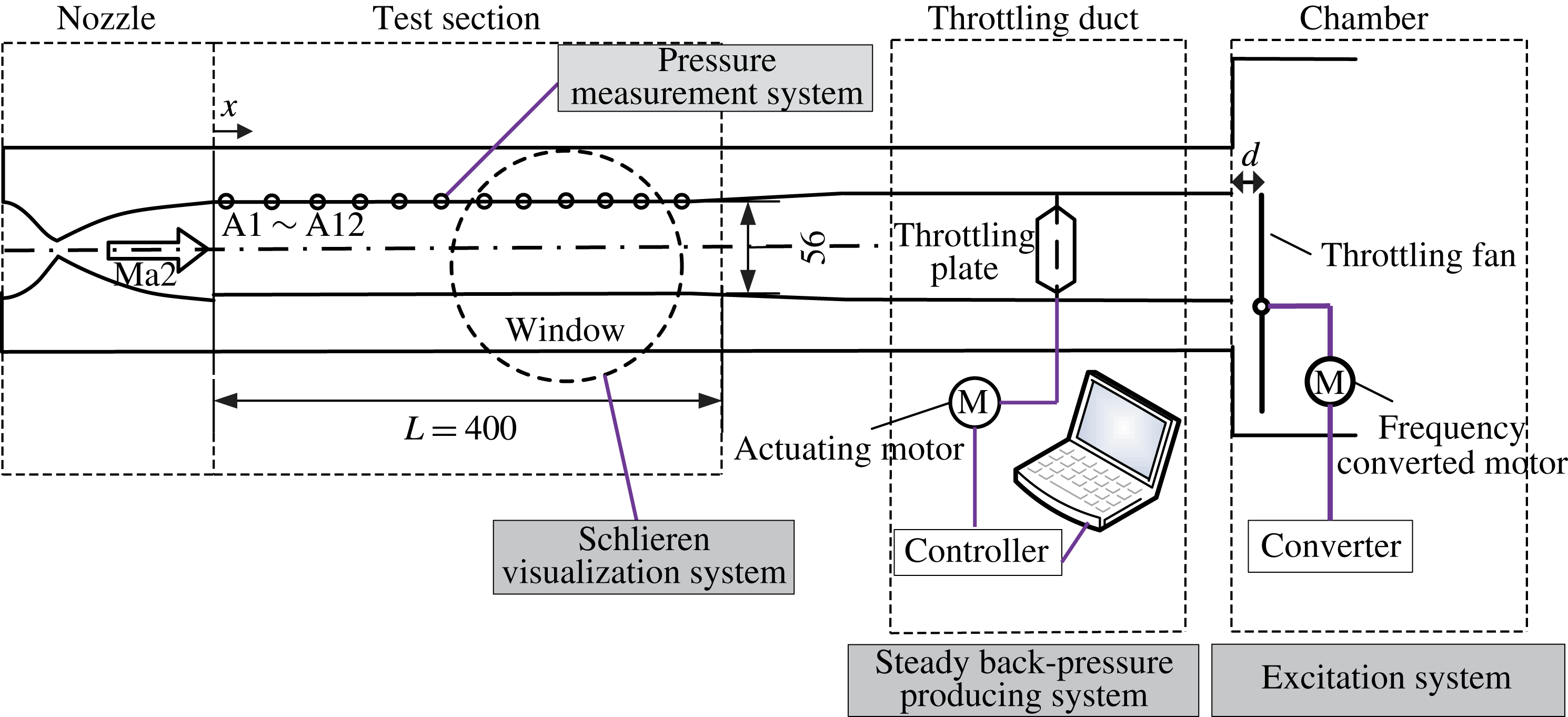
The experiments were conducted in a supersonic and air-breathing wind tunnel of the National University of Defense Technology’s Scramjet Laboratory. Figure 1 shows the schematic diagram of wind tunnel. The test section is a rectangular constant-area duct with a height of 56 mm and a span of 120 mm, and the total length of the duct is 400 mm. The reference location
 $x=0$
is defined as the inlet of test section, as shown in figure 1. A Mach 2 nozzle is installed upstream of test section.
Schematic diagram of the test set-up. The incoming Mach number is 2.0. The steady back pressure was produced by the throttling plate and downstream periodic excitations were generated by the rotating fan.

In order to form a shock train in this duct, a plate is placed downstream of duct to throttle the flow. The shock train position is adjustable by changing the throttling ratio. An excitation system is located in a downstream position, which includes a throttling fan, a motor and a converter. The throttling fan is powered by a motor and is able to rotate periodically to produce periodical excitations. In this experiment, the stagnation pressure of the incoming flow is
 $101.3~\text{kpa}\pm 0.5~\text{kpa}$
, and the stagnation temperature is
 $288~\pm 1.5~\text{K}$
.
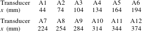
The 12 transducers labelled A1–A12 were placed along the upper wall of the duct, and the
 $x$
-locations for 12 transducers are presented in table 1. A sampling rate of 1 kHz was used to capture the instantaneous pressure along the wall. A Z-type Schlieren system was used to snap the shock train motions. The optical window is shown as dashed circle presented in figure 1. In each test, high-speed images are captured using a Photron Fastcam SA5 high-speed camera fitted with a 105 mm lens at a frame rate of 1 kHz and a resolution of
 $768\times 512$
pixel sensitivity.
The
 $x$
-locations for 12 transducers along the duct wall.

3 Experimental results
3.1 Shock train behaviours for a steady case
Shock train behaviours for a steady case were estimated briefly before studying the unsteady shock train motions. In the test case, a steady back pressure was applied to form a shock train and make sure that the shock train can be captured through the optical window.
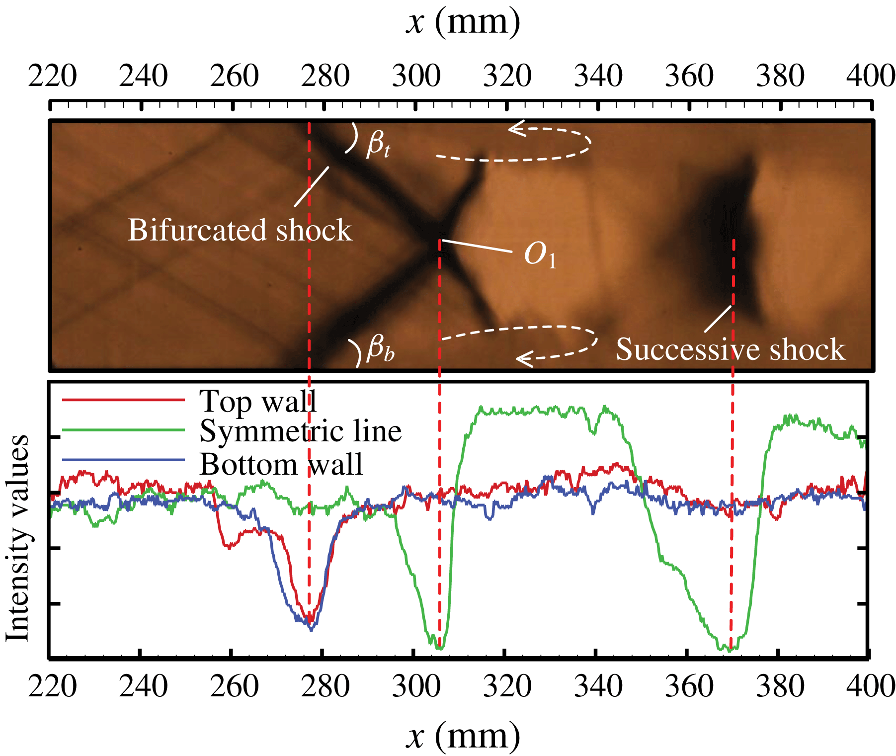
Figure 2 presents an instantaneous Schlieren image of the shock train. Under a Mach 2 incoming condition, the shock train behaves as a normal one. A first bifurcated shock and then a successive normal shock were captured. Two separation bubbles, which are marked with dashed lines in figure 2, form at the foot of separated shocks for the top wall and the bottom wall.
The Schlieren image of a shock train for a steady case. The image intensity values along the top wall, bottom wall and the symmetric line are plotted blow.
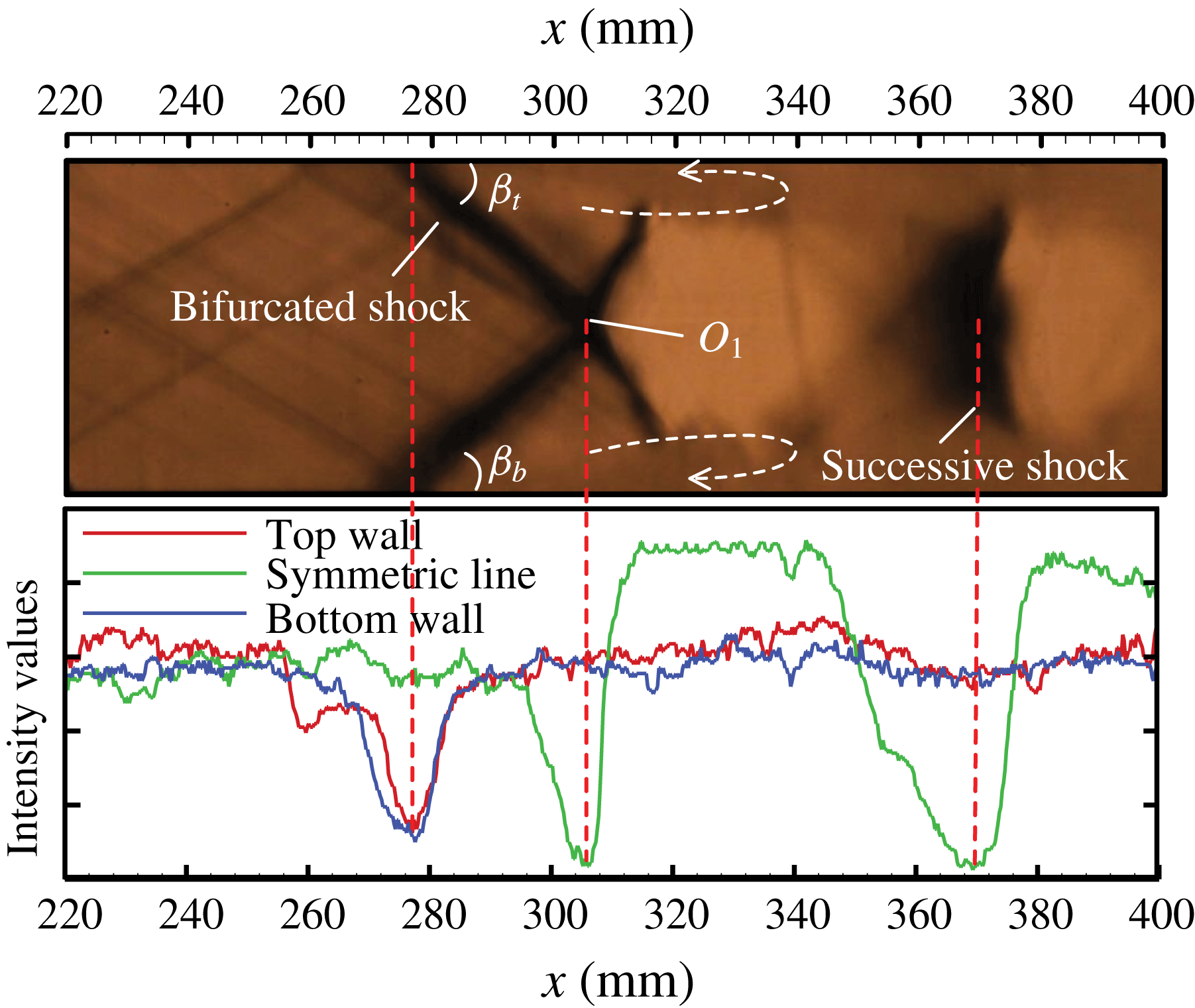
A line-scanning technology was applied to analyse the shock train structure quantitatively. The image intensity value distributions along the top wall, the bottom wall and the symmetric line are plotted below the Schlieren image. Locations of the shock train leading edge (STLE), the three-crossing point
 $O_{1}$
and the second shock can be judged from intensity value distributions with an accuracy based on pixel size of 0.2 mm. Table 2 shows the coordinates of some key points in the shock train.
 $t_{STLE}$
and
 $b_{STLE}$
are the shock train leading edge along the top wall and the bottom wall respectively. From table 2, the separated shock angles for the top wall and the bottom wall were computed as
 $44.0^{\circ }$
and
 $44.4^{\circ }$
, which implies that the shock train shows a symmetric structure.
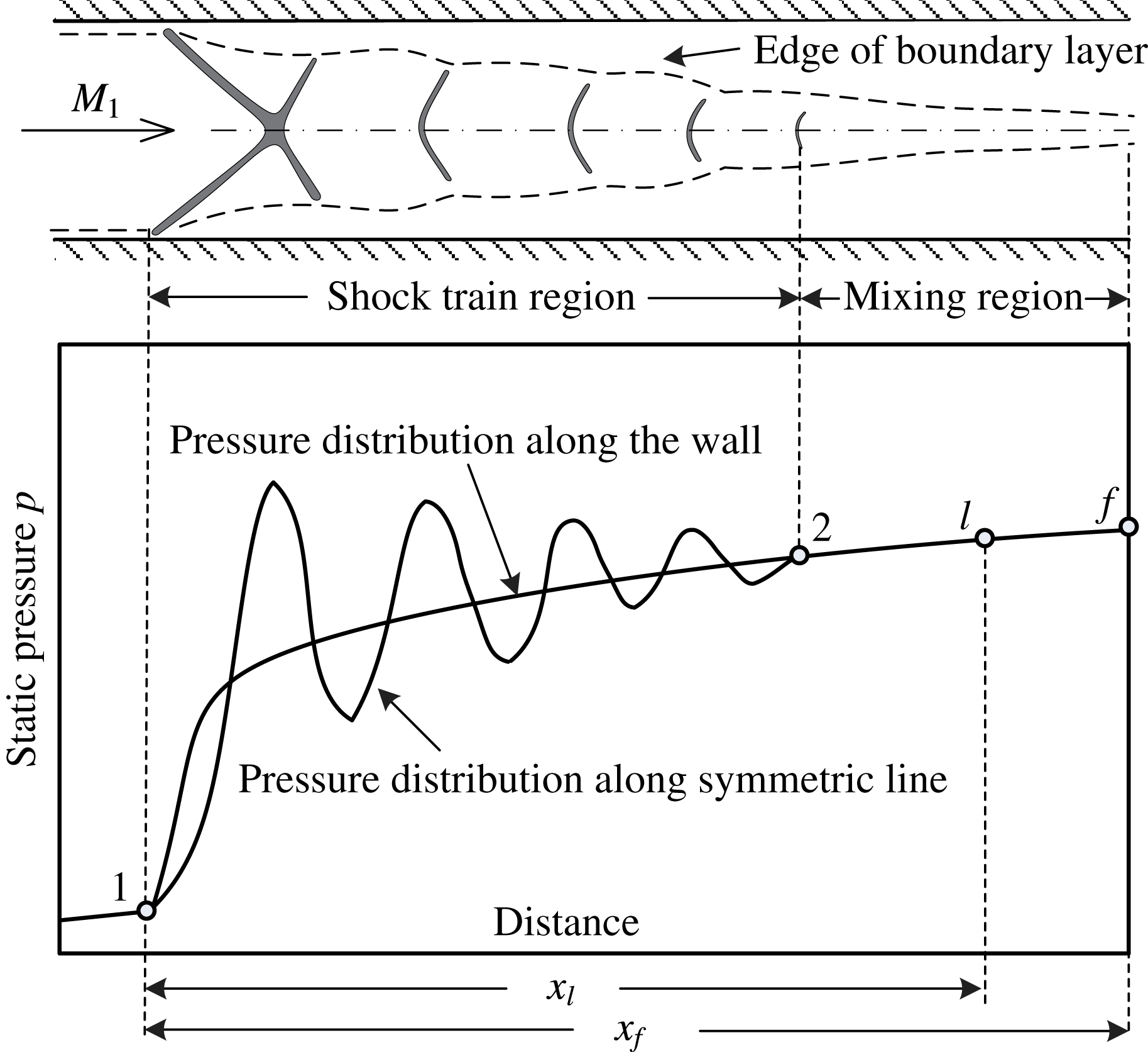
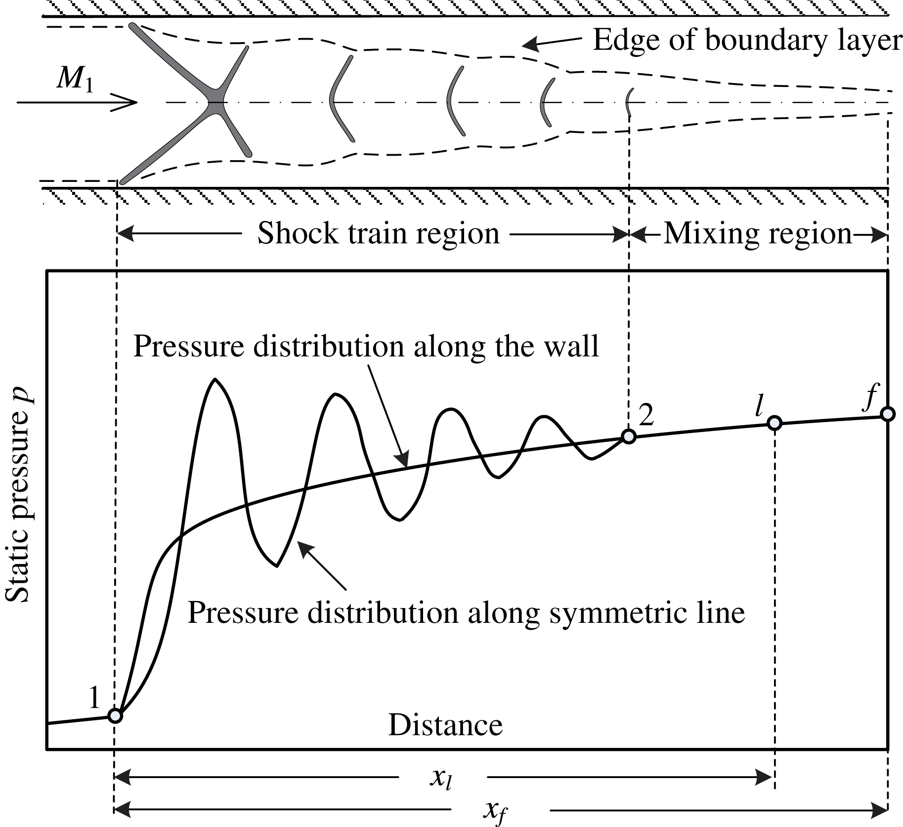
Figure 3 presents a normal shock train schematically. The corresponding static pressure distributions along the wall and the symmetric line are also plotted in this figure. As can be seen, the wall pressure starts to rise at the STLE (point 1) and increases to the end of mixing region (point
 $f$
). The pressure along the symmetric line fluctuates in the shock train region, which consists of a series of shocks. More detailed descriptions about the shock train flow fields have been previously given by Matsuo, Miyazato & Kim (Reference Matsuo, Miyazato and Kim1999).
Schematic illustrations of a symmetric shock train and the corresponding pressure distributions along the wall and the symmetric line.
 $x_{l}$
and
 $x_{f}$
are the distances from the starting point of the wall pressure rise.
The information for shock train structure determined using the image processing method.

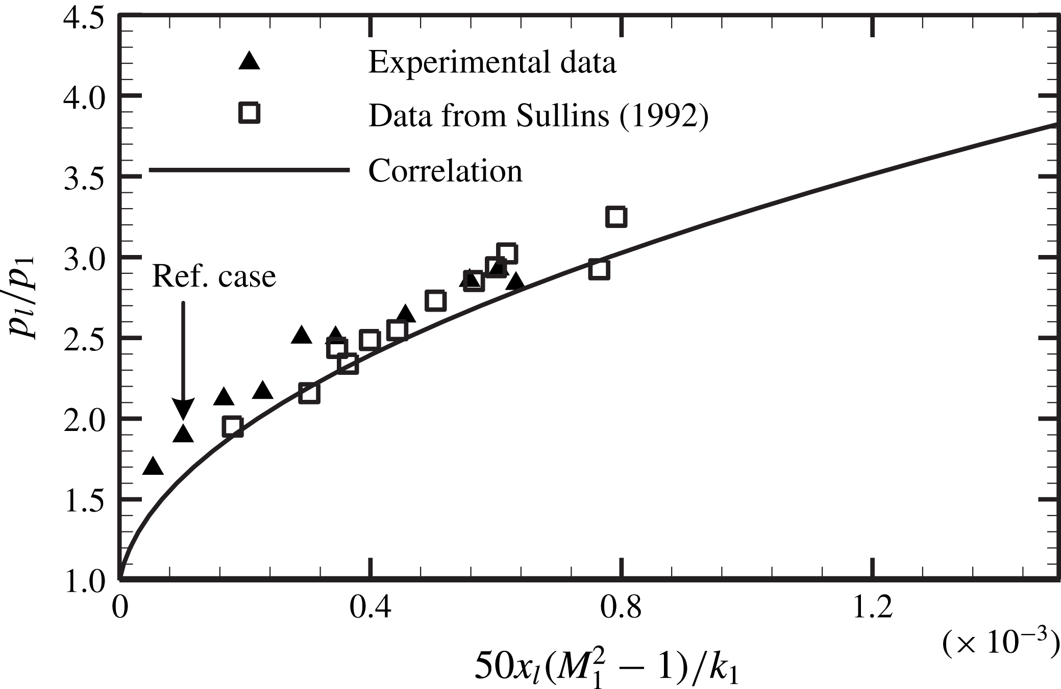
In a previous study, Waltrup & Billig (Reference Waltrup and Billig1973) developed an empirical correlation between the wall pressure distribution and several duct flow parameters in a cylindrical duct. In 1992, this correlation was developed for shock trains in the rectangular duct by Sullins (Reference Sullins1992), and the new correlation was presented as:
 $$\begin{eqnarray}(M_{1}^{2}-1)x_{l}=k_{1}\left(\frac{p_{l}}{p_{1}}-1\right)+3.4k_{1}\left(\frac{p_{l}}{p_{1}}-1\right)^{2},\end{eqnarray}$$
where
 $k_{1}=50(\sqrt{\unicode[STIX]{x1D703}H}/Re_{\unicode[STIX]{x1D703}}^{0.2})$
,
 $x_{l}$
is the distance from the beginning of pressure rise point
 $1$
,
 $M_{1}$
is incoming Mach number,
 $H$
is the height of the duct,
 $\unicode[STIX]{x1D703}$
is the momentum thickness of boundary layer for the undisturbed flow,
 $Re_{\unicode[STIX]{x1D703}}$
is the Reynolds number based on
 $\unicode[STIX]{x1D703}$
and
 $p_{l}/p_{1}$
is the ratio of local wall pressure to the pressure at the STLE position. This correlation was widely used in the constant-area isolator to predict the wall pressure distribution or the length of a shock train. Figure 4 compares our experimental results and this correlation. It can be seen that the pressure rise
 $p_{l}/p_{1}$
in our test cases can be well predicted by this correlation. Figure 4 or (3.1) implies that the existence of a shock train in the duct is to match the pressure rise, the larger the pressure rise
 $p_{l}/p_{1}$
is, the longer the shock train will be. Therefore, the mechanism for shock train matching the pressure rise for steady cases is that the shock train fits the shock train length or the STLE position to match a new imposed pressure rise. However, whether this mechanism is suitable for unsteady cases is unclear, and it will be discussed in following sections.
The comparison between our experimental results and correlation equation (3.1).

3.2 Response of a shock train to downstream excitations
To estimate the characteristics of the unsteady shock train motions, a fluctuating back pressure with an excited frequency 75 Hz was applied downstream of the duct using the excitation system.
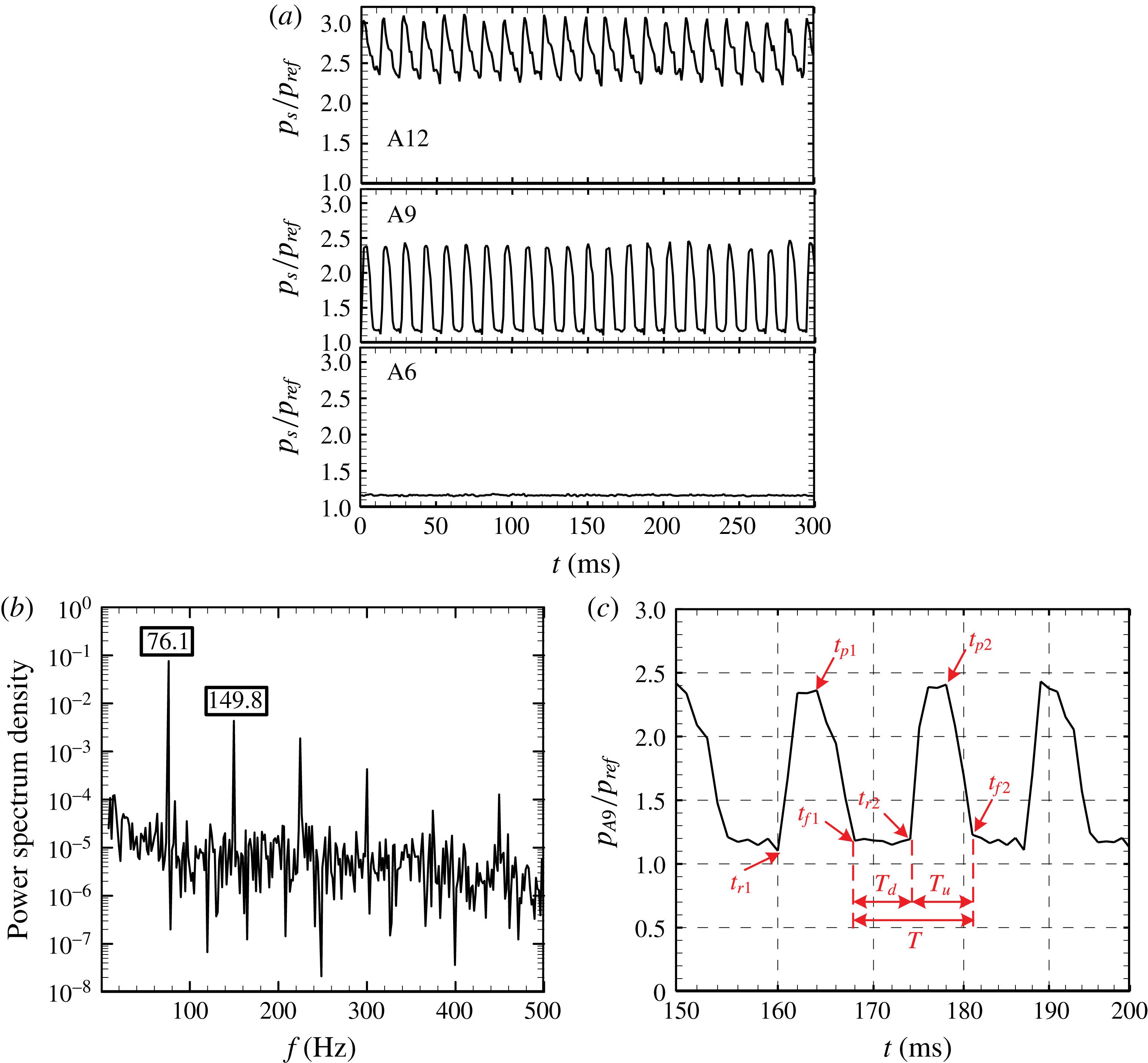
Figure 5(a) shows pressure histories at several locations along the duct, and the pressure is normalized by
 $p_{ref}$
, which is 13 kPa. It can be seen that the pressure at A12, which is located near the outlet of the duct, shows obvious periodical behaviour due to downstream excitations. The frequency characteristics for A12 were obtained with the fast Fourier transform (FFT) method, and the power spectrum density (PSD) results are presented in figure 5(b). This shows that the pressure fluctuates at a dominant frequency 76.1 Hz, which is very close to the excitation frequency of 75 Hz. The several successive peaks, such as at 149.8 Hz, correspond to harmonics of the excitation.
(a) The pressure histories for A12, A9 and A6 when subjected to downstream excitations. (b) The PSD distribution for A12 where the dominant frequency is 76.1 Hz. (c) The pressure history for A9 between 150 and 200 ms; the shock train motions can be judged from pressure fluctuations.

The pressure fluctuations at A9 show obvious periodical and intermittent behaviours, which are induced by periodical shock train motions. Figure 5(c) gives the pressure history at A9 between 150 and 200 ms. It is found that the shock train motions are associated with pressure fluctuations and the shock train location can be judged from the pressure signals. At
 $t_{f1}=168.0$
ms, the shock train is located at the most downstream position and starts to move upstream, thus the pressure at A9 is maintained at an undisturbed level. At
 $t_{r2}=174.0$
ms, the shock train travels across A9 and moves upstream continuously, which leads to the pressure spikes at
 $t_{r2}$
. At
 $t_{p2}=178.0$
ms, the shock train is located at the most upstream position and turns back. By
 $t_{f2}=181.0$
ms, the cyclic motion is finished, and the period time
 $T$
equals 13 ms (
 $1/T=76.9$
Hz).
The pressure at A6 stays almost steady, and it is not affected by the shock train motions. This implies that the moving shock train can isolate the interactions between the downstream excitations and the incoming flow.
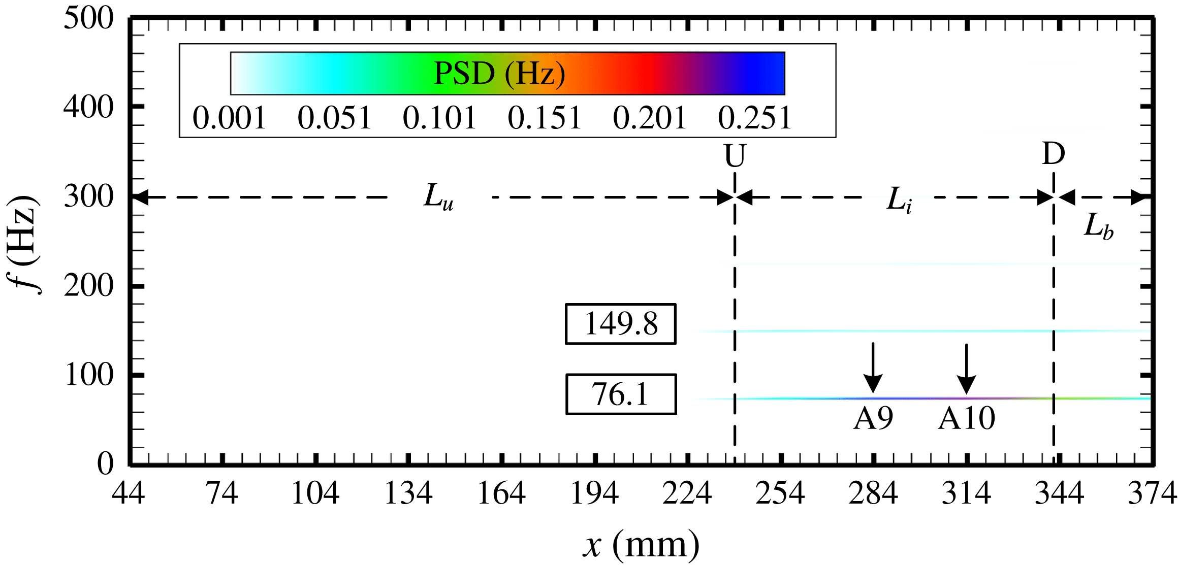
Figure 6 presents the spatial frequency distribution along the duct wall, and the contour image is coloured with pressure PSD values. In figure 6, U and D indicate the mean extreme upstream and mean extreme downstream positions of the shock train respectively, which will be discussed in detail in the following. According to the pressure behaviours, the whole duct is divided into three regions. The undisturbed region, of length
 $L_{u}$
, is located upstream of position U. Pressures in this region are not affected by the shock train oscillations and are almost steady (like A6). The intermittent region, of length
 $L_{i}$
, is located between positions U and D. Pressures in this region are violently affected by the shock train motions and show obvious intermittent behaviours (like A9). The back-pressure affected region, of length
 $L_{b}$
, is located downstream of position D. Pressures in this region are essentially affected by both the shock train motions and the downstream excitations.
It can be seen in this figure that a dominant frequency of 76.1 Hz and its harmonic at 149.8 Hz were found in both the intermittent region and the back-pressure affected region. This implies that the shock train oscillates at the excited frequency and the oscillation is mainly a forced one. Moreover, it means that the downstream disturbance produced by the excitation system could travel to the counterflow direction and affect the shock train motions. Some parts of the core flow are supersonic, through which disturbances cannot travel upstream, so pressure disturbances may travel through the subsonic boundary layer.
The spatial frequency distributions along the duct wall. The dominant frequency is 76.1 Hz. The whole duct is divided into three regions, the undisturbed region
 $L_{u}$
, the intermittent region
 $L_{i}$
and the back-pressure affected region
 $L_{b}$
.

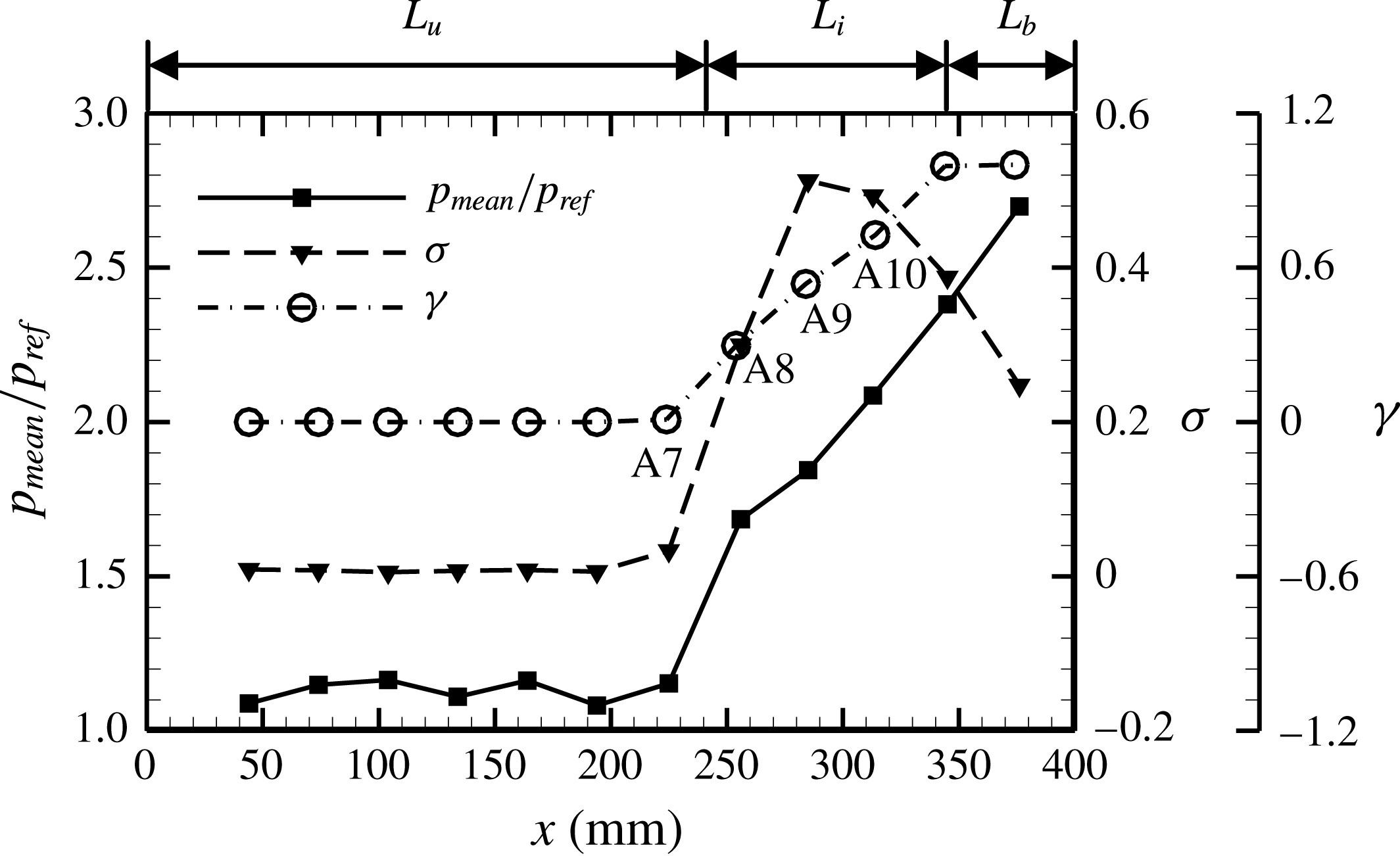
The distributions of mean pressure, pressure standard deviation and intermittent factor along the duct wall.

To estimate more characteristics of the forced shock train oscillation, the distributions of the mean pressure, the pressure standard deviation
 $\unicode[STIX]{x1D70E}$
, and the intermittent factor
 $\unicode[STIX]{x1D6FE}$
are presented in figure 7. The pressure standard deviation is defined as:
 $$\begin{eqnarray}\unicode[STIX]{x1D70E}=\sqrt{\frac{\displaystyle \mathop{\sum }_{i=1}^{N}(p_{i}-p_{mean})^{2}}{N-1}},\end{eqnarray}$$
where
 $p_{mean}$
is the mean pressure measurement and
 $N$
is the number of samples. The intermittent factor is defined as:
 $$\begin{eqnarray}\unicode[STIX]{x1D6FE}=\frac{1}{t_{total}}\mathop{\sum }_{i=1}^{n}(t_{fi}-t_{ri}),\end{eqnarray}$$
where
 $t_{f}$
and
 $t_{r}$
are shown as figure 5(c),
 $t_{total}$
is the total time of a test case. The intermittent factor is the percentage of the STLE that is located upstream of a transducer during the total time. Taking A9 for example (in figure 5
c), the STLE is located upstream of A9 during time
 $T_{u}$
, so the intermittent factor in this period is
 $T_{u}/T=0.54$
. Thus,
 $\unicode[STIX]{x1D6FE}$
for the undisturbed region is 0 and for the back-pressure affected region is 1, as presented in figure 7.
In the intermittent region, the pressure standard deviation
 $\unicode[STIX]{x1D70E}$
obtains its peak value at A9, and it is interesting that the intermittent factor at A9 is 0.54. Essentially, the trend of the
 $\unicode[STIX]{x1D70E}$
distribution is decided by the
 $\unicode[STIX]{x1D6FE}$
value. In an oscillation circle, the STLE travels through a position twice, from downstream or upstream direction, and this leads the pressure at this position to rise to a high level or fall to an undisturbed level (as shown in figure 5
c). As a result, the pressure shows the most serious deviation from the average level, which means that the standard deviation reaches the peak value when the intermittent factor is 0.5. Thus,
 $\unicode[STIX]{x1D70E}$
will experience a uptrend when
 $\unicode[STIX]{x1D6FE}$
increases from 0 to 0.5, and then experience a downtrend when
 $\unicode[STIX]{x1D6FE}$
increases from 0.5 to 1, as illustrated in figure 7.
To estimate more characteristics of unsteady shock train motion, the history of shock train movements was recorded and analysed. The shock train motions were recorded through a fixed optical window, as shown in figure 1. However, it is difficult to control the range of shock train movement to make sure that the shock train can be captured in a whole period. That is to say, the shock train may move out of optical sight for parts of a period. As a result, the whole history of the STLE positions cannot be obtained using image processing technology in most test cases. A pressure ratio method was utilized here to relieve this problem. This is a method used to locate the STLE position based on pressure signals. For the STLE location in a rectangular duct, the pressure ratio method has been proved accurate and effective (see Hutzel et al. Reference Hutzel, Decker, Cobb, King and Veth2011), and it has been applied to locate the STLE for cases where the Schlieren technology is unavailable (see Hutzel et al. Reference Hutzel, Decker, Cobb, King and Veth2011; Hu et al. Reference Hu, Chang, Qin and Wang2013). The location formulas for the pressure ratio method are shown by (3.4)–(3.5):
 $$\begin{eqnarray}\displaystyle & \displaystyle \boldsymbol{P}\boldsymbol{R}(k\unicode[STIX]{x0394}t)=\left[\frac{p_{s,A1}(k\unicode[STIX]{x0394}t)}{p_{tare,A1}},\frac{p_{s,A2}(k\unicode[STIX]{x0394}t)}{p_{tare,A2}},\ldots ,\frac{p_{s,A12}(k\unicode[STIX]{x0394}t)}{p_{tare,A12}}\right] & \displaystyle\end{eqnarray}$$
 $$\begin{eqnarray}\displaystyle & \displaystyle x_{STLE}(k\unicode[STIX]{x0394}t)=\text{interp}(\boldsymbol{P}\boldsymbol{R}(k\unicode[STIX]{x0394}t),\boldsymbol{x}_{trans},PR_{des}), & \displaystyle\end{eqnarray}$$
where vector
 $\boldsymbol{P}\boldsymbol{R}(k\unicode[STIX]{x0394}t)$
is made of the pressure ratios for each transducer,
 $p_{tare}$
means the pressure measurement in the undisturbed phase, vector
 $\boldsymbol{x}_{trans}$
is made up of the transducer locations and
 $PR_{des}$
is the desired pressure ratio as well as the interpolation point, which is 1.5 for a Mach 2 incoming condition (see Le et al.
Reference Le, Goyne and Krauss2008; Hutzel et al.
Reference Hutzel, Decker, Cobb, King and Veth2011).
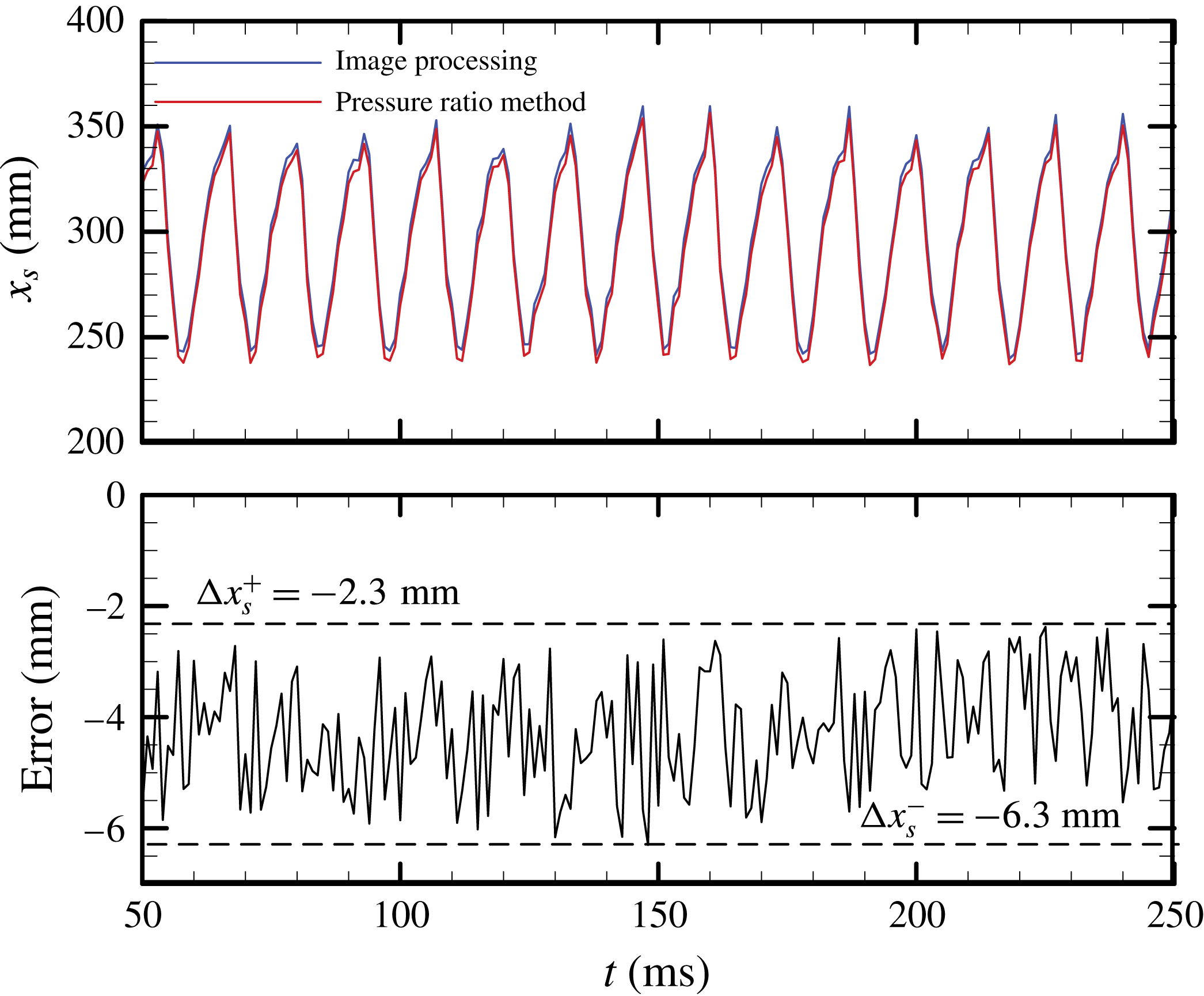
To confirm the pressure ratio method for our test condition as well as determine the errors of this method, the sequential STLE positions obtained with the pressure ratio method and the line-scanning technology were compared in figure 8. The STLE position located with the image processing method is regarded to be exact, and the history of error
 $\unicode[STIX]{x0394}x_{s}$
is shown in figure 8. It can be seen that the maximum deviation from the image processing results is
 $\unicode[STIX]{x0394}x_{s}=-6.3$
mm and the minimum deviation is
 $\unicode[STIX]{x0394}x_{s}=-2.3$
mm. Compared with the range of shock train oscillations (more than 100 mm), the error of the pressure ratio method is acceptable. Thus, the pressure ratio method is utilized to locate the STLE position for our test cases, and the error bar is
 $\unicode[STIX]{x0394}x_{s}\unicode[STIX]{x1D716}$
(
 $-$
6.3 mm,
 $-$
2.3 mm). This means that the position determined with the pressure ratio method is inherently located more upstream than the actual position, which was previously found in the research of Hutzel et al. (Reference Hutzel, Decker, Cobb, King and Veth2011).
The instantaneous STLE positions located with the pressure ratio method and the line-scanning technology at excited frequency 75 Hz. The corresponding errors are presented below.

3.3 Mechanism of unsteady shock train motions
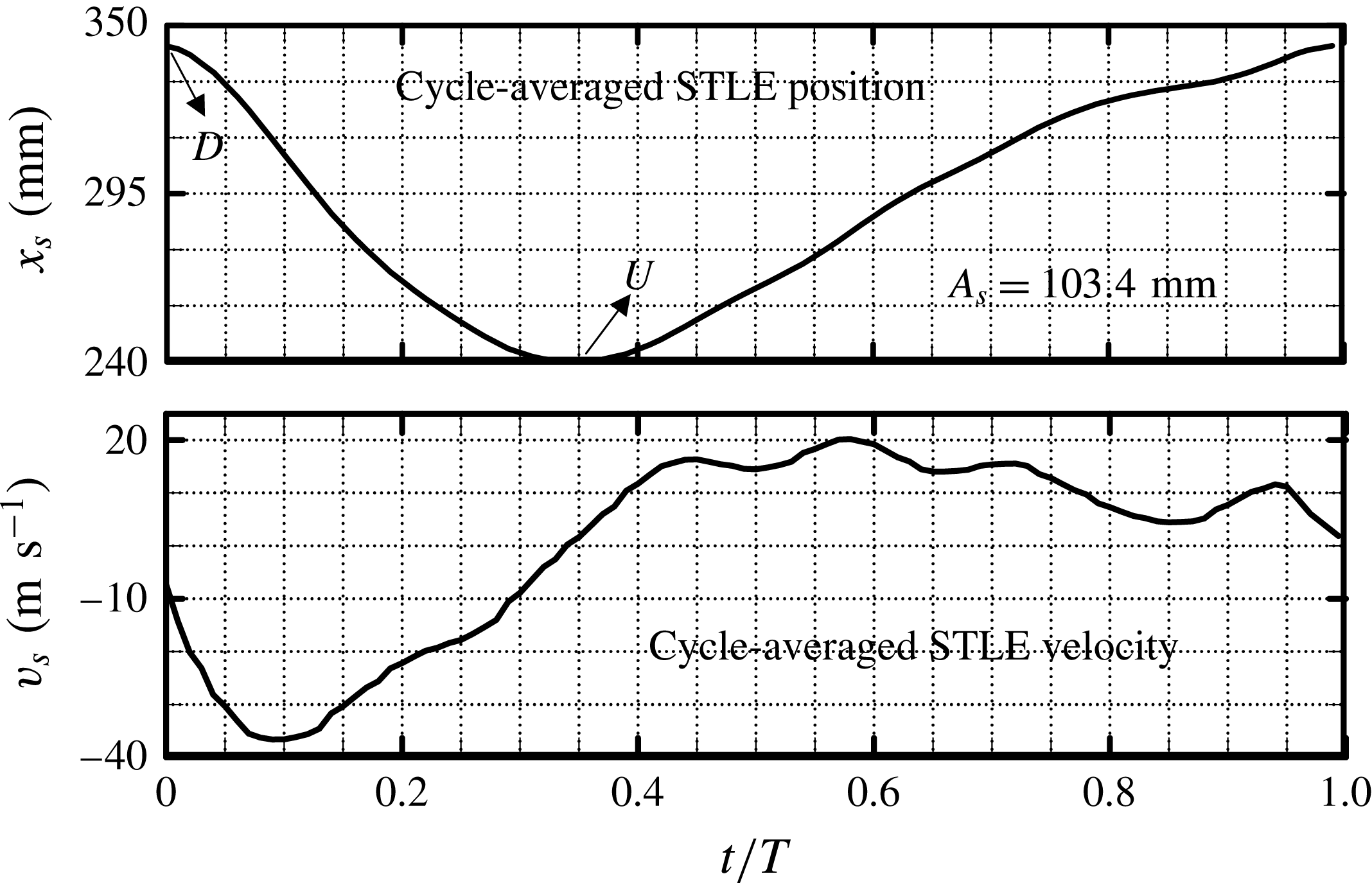
Figure 8 clearly shows periodical motions of the shock train, although each cycle is not absolutely repeatable. Several seconds of unsteady shock train motions were recorded to calculate an averaged cycle. The cycle-averaged STLE position, computed from the result of the pressure ratio method, is illustrated in figure 9. The corresponding cycle-averaged STLE velocity is also presented here, and the time is normalized by the averaged oscillation period. It can be found that the shock train is located at the most downstream position (U:
 $x_{s}=240.0$
mm) at
 $t/T=0$
and arrives at the most upstream position (D:
 $x_{s}=343.4$
mm) at
 $t/T=0.36$
, where its velocity is approximately 0. At
 $t/T=1$
, the shock train has arrived at the most downstream position again and has finished an oscillation cycle. The mean amplitude of the shock train oscillation
 $A_{s}$
is defined as the distance between the mean most upstream (U) and most downstream position (D), and it is
 $103.4\pm 4.0$
mm for this test case.
The cycle-averaged STLE position and velocity cycle at excited frequency 75 Hz. The cycle-averaged amplitude of the shock train oscillation is
 $103.4\pm 4.0$
mm.

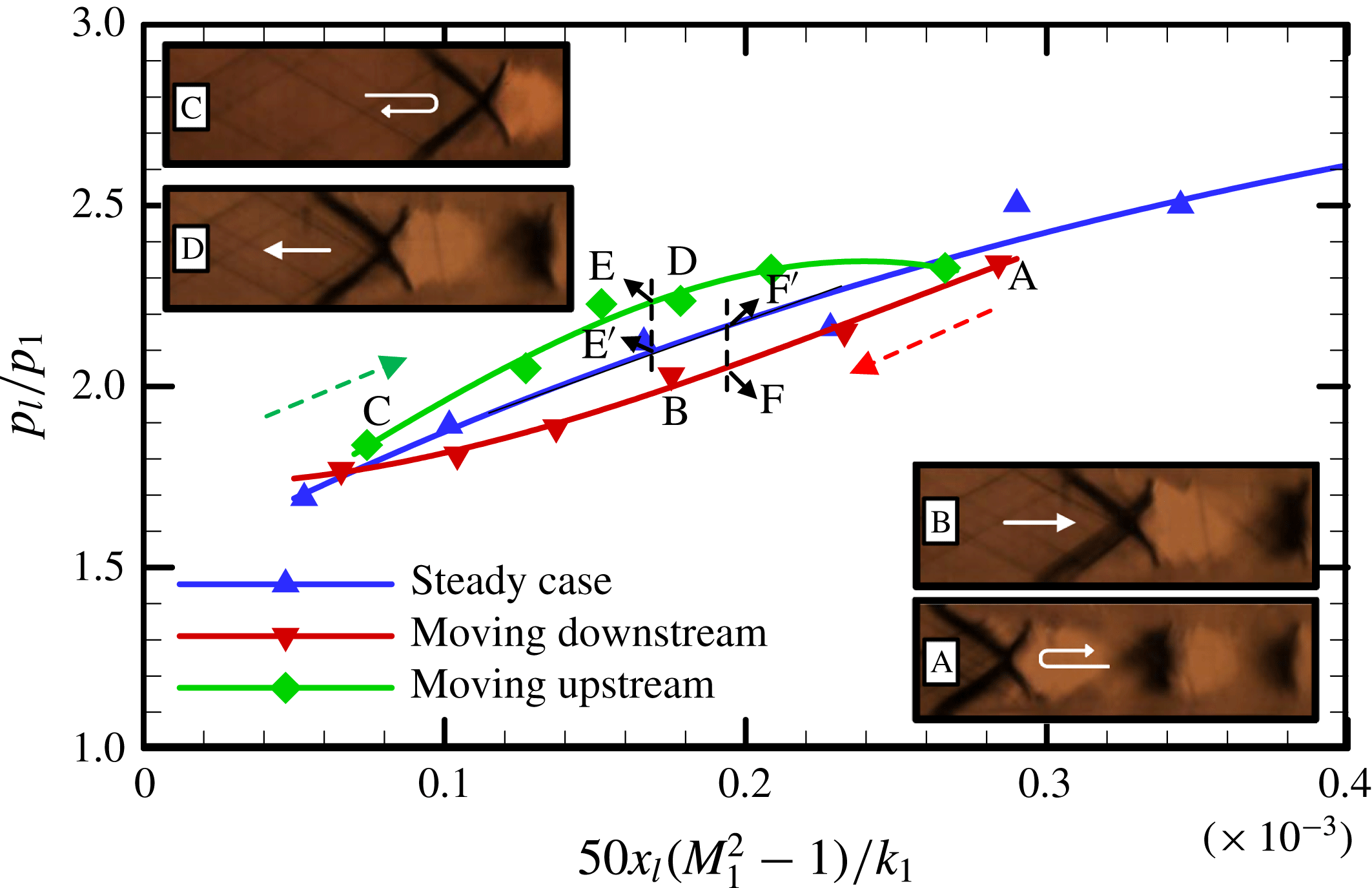
Figure 10 presents the correlation between STLE positions and the pressure rise for a specific motion cycle. For comparison, the results for steady cases (see figure 4) are plotted here again. Lines plotted in figure 10 are trend lines of the experimental data. The Schlieren images show instantaneous shock train structures captured in a motion cycle. Image A shows the most upstream shock train, which was taken with a bifurcated shock train and two successive shocks, and a highest pressure rise was induced by this shock train position. Image C shows the most downstream shock train, which was only taken with a bifurcated shock train, and the induced pressure rise reaches the lowest.
The correlation between STLE positions and pressure rises for a specific motion cycle. The data during the upstream and downstream movement are plotted in red and green respectively. The corresponding Schlieren images are marked with A, B, C and D.

Images B and D show the shock train located at almost the same position when travelling downstream and upstream respectively. Figure 10 illustrates that the pressure rise induced by the upstream-moving (D) shock train is much larger than induced by the downstream-moving shock train (B). The pressure rise induced by the steady shock train lies between B and D. This may be attributed to the changes of the relative Mach number, in which the speed of the shock train is considered, ahead of the shock train. During the upstream motion, the shock train moves in the opposite direction to the incoming flow, so the relative Mach number ahead of shock train is larger than
 $M_{1}$
. As a result, the pressure rise induced by the upstream-moving shock train is larger than that of the steady cases. As for the downstream motion, the relative Mach number ahead of the shock train is smaller than
 $M_{1}$
, thus leading to a lower pressure rise. Moreover, figure 10 shows that the pressure rises induced by the most upstream shock train (A) and the most downstream shock train (C) are almost equal to the pressure rise for the steady case. This may be attributed to the low moving speed of shock train. For steady cases, the pressure rise is decided by the absolute incoming Mach number
 $M_{1}$
when the STLE is located at the same position, as illustrated in (3.1) or figure 4.
Figure 10 shows that there is an obvious deviation between the pressure rises induced by a moving shock train and a steady shock train, when they are located at the same position. Moreover, this deviation is greatly affected by the shock train moving speed as well as the moving direction (to upstream or downstream). During the upstream movement, the maximum pressure rise deviation is between level E and level E
 $^{\prime }$
. The pressure rise induced by an upstream-moving shock train is 2.23 (level E), which is 6.19 % larger than the steady pressure rise 2.10 (level E
 $^{\prime }$
). According to (3.1), it can be inferred that the ‘needed’ incoming Mach number for the pressure rise of 2.23 is
 $M_{1r}=2.17$
(at the same STLE position) for a steady case. That is to say, the pressure rise of 2.23 will be induced by an incoming Mach 2.17 flow for a steady case with the same effect. For unsteady cases,
 $M_{1r}=2.17$
means the relative Mach number ahead of a shock train is 2.17, and it is predicted that the maximum shock train moving Mach is
 $M_{s}=-0.17$
(to the upstream direction). Then, the predicted or needed velocity for shock train upstream movement is approximately
 $-43.1~\text{m}~\text{s}^{-1}$
(the sound speed is
 $253.55~\text{m}~\text{s}^{-1}$
). The experimental maximum moving speed during the upstream motion is
 $-36.6~\text{m}~\text{s}^{-1}$
, as shown in figure 9, which is 15.1 % smaller than the predicted value. During the downstream movement, the maximum pressure rise deviation is between level F and level F
 $^{\prime }$
. The pressure rise induced by a downstream-moving shock train is 2.05 (level F), which is 4.21 % smaller than the steady pressure rise of 2.14 (level F
 $^{\prime }$
). Similar to the above analysis, the relative Mach number ahead of the shock train is computed as 1.89. So, it is predicted that the maximum shock train moving Mach is
 $M_{s}=0.11$
(to the downstream direction). Then, the predicted or needed velocity for shock train downstream movement is approximately
 $27.9~\text{m}~\text{s}^{-1}$
. The experimental maximum moving speed during the downstream motion is
 $20.2~\text{m}~\text{s}^{-1}$
, as shown in figure 9, which is 27.6 % smaller than the predicted value.
The deviation between the predicted shock train velocity and the experimental value may occur for two reasons. One is that the experiment velocity presented in figure 9 is a mean result, and the predicted velocity comes from a specific period. Another is the error from the prediction of the maximum and minimum pressure rise due to the trend lines. Although there exist errors, it can be confirmed from figure 10 that the difference in the pressure rise induced by a moving shock train and a steady shock train, which are located at the same position, may be attributed to the change of relative Mach number.
From what has been analysed above, the shock train moving speed has a great effect on the pressure rise induced by the shock train, through changing the relative Mach number ahead of the shock train. From this, it can be concluded that the mechanism by which the shock train responds to downstream excitations is to keep moving so that the relative Mach number ahead of the shock train changes to match the varying imposed back pressure. From (3.1) and figure 4, it is known that the shock train changes its position to match a back-pressure variation for the steady case. Therefore, the above analysis suggests that the mechanism for the unsteady shock train matching the imposed back-pressure variations is very different from the steady cases, where a shock train changes the STLE position to match a downstream pressure jump. The concept of relative Mach number
 $M_{r}$
is very important for the modelling of unsteady shock train motions, which will be illustrated in the following.
4 Modelling of unsteady shock train motions
4.1 Analytical study
To predict the unsteady shock train motion, a simple analytical study of a normal shock train in a constant-area rectangular duct when subjected to downstream pressure excitations was conducted.
The shock train moves in response to a downstream disturbance in an infinitesimal time.

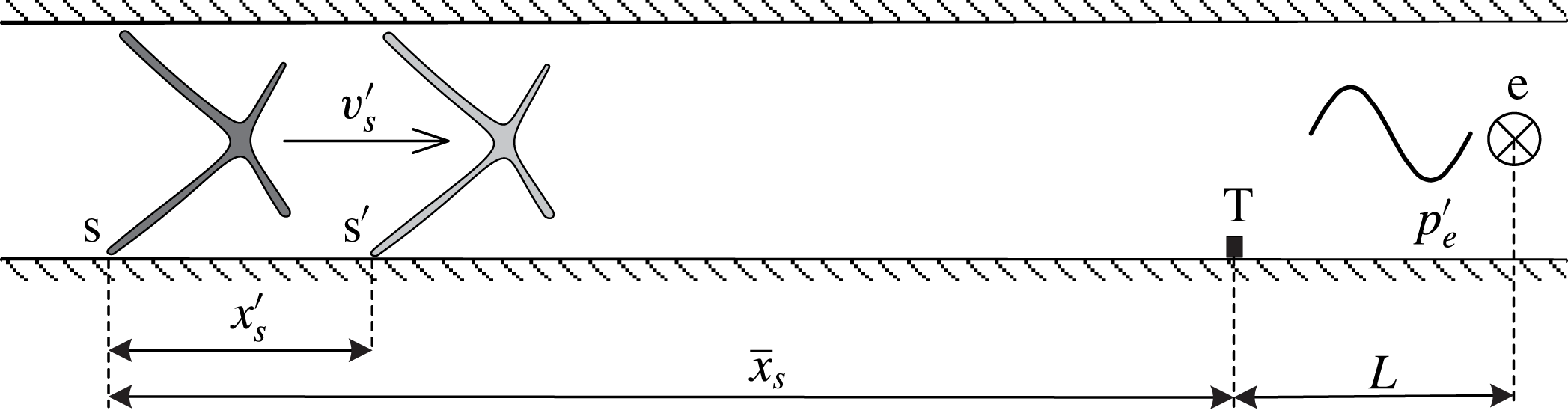
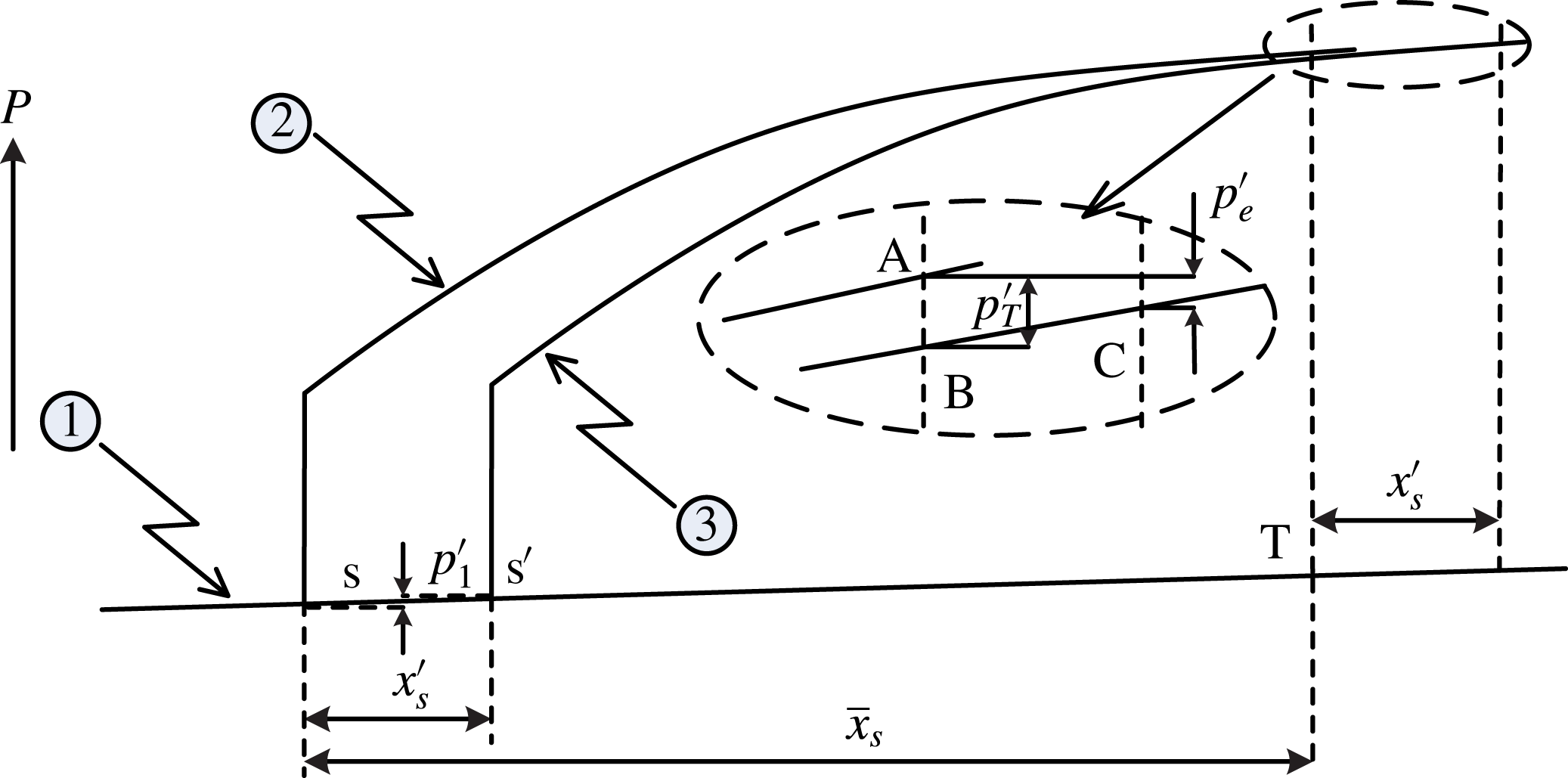
Figure 11 schematically shows the response of the shock train to a pressure disturbance in an infinitesimal time, and a bifurcated shock is shown here to represent the whole shock train. The position s is where the STLE is located for the steady case, and T is a pressure measuring point. According to the above analysis, the correlation between length
 $\overline{x}_{s}$
and pressure ratio
 $p_{T}/p_{1}$
can be predicted with (3.1). The position
 $\text{e}$
is where the downstream excitation is located, and the distance between T and e is
 $L$
. Based on the steady case, a pressure disturbance
 $p_{e}^{\prime }$
produced by the excitation system can travel upstream. As a result, the shock train moves from position s to position s
 $^{\prime }$
and the displacement of shock train is
 $x_{s}^{\prime }$
, as shown in figure 11. During the moving process, the flow is strictly unsteady. For a good approximation, the quasi-steady assumption is applied for the moving process. Thanks to the quasi-steady assumption, we may analyse the forced shock train oscillation, which is a totally unsteady behaviour, by applying the correlation illustrated in (3.1) to the instantaneous flow parameters. Culick & Rogers (Reference Culick and Rogers1983) first used the quasi-steady assumption to analyse the unsteady normal shock in a diffuser. Bruce & Babinsky (Reference Bruce and Babinsky2008) also used this assumption to analyse the unsteady shock dynamics in a parallel-walled duct. The shock train moves in response to a downstream disturbance, and the velocity of the upstream flow changes for two reasons. On the one hand, it is brought about by the shock train velocity fluctuations
 $v_{s}^{\prime }$
(to the opposite direction). On the other hand, when the shock train location fluctuates
 $x_{s}^{\prime }$
, the boundary layer thickness ahead of the shock train changes as well, thus leading to a flow velocity change. So, the fluctuation of velocity of the upstream flow can be presented as the following:
 $$\begin{eqnarray}u_{1}^{\prime }=-v_{s}^{\prime }+\left.\frac{\text{d}\overline{u}_{1}}{\text{d}x}\right|_{s}\cdot x_{s}^{\prime },\end{eqnarray}$$
where
 $\overline{u}_{1}$
is the velocity of the upstream flow for the steady case. Similarly, the fluctuation of the upstream Mach number is shown as:
 $$\begin{eqnarray}M_{1}^{\prime }=-\frac{v_{s}^{\prime }}{\overline{a}_{1}}+\left.\frac{\text{d}\overline{M}_{1}}{\text{d}x}\right|_{s}\cdot x_{s}^{\prime },\end{eqnarray}$$
where
 $\overline{a}_{1}=\sqrt{\unicode[STIX]{x1D6FE}R\overline{T}_{1}}$
is the sound speed of the undisturbed flow, and
 $\overline{M}_{1}$
is the Mach number of the upstream flow for the steady case.
Schematic wall pressure distributions for the quasi-steady assumption.

Figure 12 schematically shows several static pressure distributions for the quasi-steady assumption. Line 1 represents the wall pressure distribution in the absence of a shock train, and the wall pressure increases gradually due to the naturally grown boundary layer. Line 2 and line 3 represent wall pressure distributions when the STLE is located at positions s and s
 $^{\prime }$
respectively. In this figure, the pressure rise induced by the separated shock is simplified as a vertical line. When the shock train moves from position s to s
 $^{\prime }$
, the pressure of the upstream flow
 $p_{1}$
fluctuates due to the displacement according to:
 $$\begin{eqnarray}p_{1}^{\prime }=\left.\frac{\text{d}\overline{p}_{1}}{\text{d}x}\right|_{s}\cdot x_{s}^{\prime }.\end{eqnarray}$$
The fluctuation of pressure at position T is presented as
 $p_{T}^{\prime }$
, as shown in figure 12. If the STLE is located at the original position s, the wall pressure increases to level A at position T. In the same length
 $\overline{x}_{s}$
, the wall pressure increases to level C when the STLE moves to a new position. Essentially, the shock train motion is caused by the downstream fluctuation
 $p_{e}^{\prime }$
, here a reduction of pressure. According to the quasi-steady assumption, the pressure difference between level A and level C is equalled by the downstream fluctuation
 $p_{e}^{\prime }$
, as illustrated in figure 12. Thus, the correlation between
 $p_{T}^{\prime }$
and
 $p_{e}^{\prime }$
is presented as:
 $$\begin{eqnarray}p_{T}^{\prime }=p_{e}^{\prime }+\left.\frac{\text{d}\overline{p}_{T}}{\text{d}x}\right|_{s}\cdot x_{s}^{\prime },\end{eqnarray}$$
where
 $\overline{p}_{T}$
is the pressure at position T for the steady case. All flow parameters are equal to the parameters for the steady case plus the fluctuation, that is:
 $$\begin{eqnarray}\unicode[STIX]{x1D70F}_{i}=\overline{\unicode[STIX]{x1D70F}}_{i}+\unicode[STIX]{x1D70F}_{i}^{\prime }(\unicode[STIX]{x1D70F}_{i}=x_{s},p_{1},p_{T},M_{1},\ldots ).\end{eqnarray}$$
As can be seen, the flow parameters (such as pressure, flow velocity and so on) may change due to the change of STLE position, which is induced by the naturally grown boundary layer. In a constant-area duct, the streamwise gradient of flow parameters, which are induced by the naturally grown boundary layer, upstream of the shock train is extremely small (as pressure line 1 shown in figure 12). For simplification, the streamwise gradient of the flow parameters induced by the grown boundary layer is negligible. As a result, the fluctuations presented in (4.1)–(4.3) are simplified as:
 $$\begin{eqnarray}\displaystyle & \displaystyle u_{1}^{\prime }=-v_{s}^{\prime } & \displaystyle\end{eqnarray}$$
 $$\begin{eqnarray}\displaystyle & \displaystyle M_{1}^{\prime }=-\frac{v_{s}^{\prime }}{\overline{a}_{1}} & \displaystyle\end{eqnarray}$$
 $$\begin{eqnarray}\displaystyle & \displaystyle p_{1}^{\prime }=0. & \displaystyle\end{eqnarray}$$
It can be seen from figure 3 or (3.1) that the streamwise pressure gradient at position T becomes smaller when the distance
 $\overline{x}_{s}$
becomes longer. For simplification, the streamwise pressure gradient at position T is negligible when T is located in the mixing region (see figure 3). That is to say, we used a pressure measurement, where pressure level B is very close to pressure level C, to infer the real pressure disturbance. Thus, the (4.4) is simplified as:
 $$\begin{eqnarray}p_{T}^{\prime }=p_{e}^{\prime }.\end{eqnarray}$$
According to the quasi-steady assumption, the correlation between the pressure ratio
 $p_{T}/p_{1}$
and the distance
 $x_{s}$
when the shock train is located at the new position can be also presented as (3.1). Substituting (4.5)–(4.9) into (3.1), the results are:
 $$\begin{eqnarray}(\overline{M}_{1}^{2}-1)x_{s}^{\prime }+2\overline{M}_{1}\overline{x}_{s}M_{1}^{\prime }=k_{1}\frac{p_{e}^{\prime }}{\overline{p}_{1}}\left(6.8\frac{\overline{p}_{T}}{\overline{p}_{1}}-5.8\right).\end{eqnarray}$$
Substituting (4.7) into (4.10), that is:
 $$\begin{eqnarray}(\overline{M}_{1}^{2}-1)x_{s}^{\prime }-\frac{2\overline{M}_{1}\overline{x}_{s}}{\overline{a}_{1}}v_{s}^{\prime }=k_{1}\frac{p_{e}^{\prime }}{\overline{p}_{1}}\left(6.8\frac{\overline{p}_{T}}{\overline{p}_{1}}-5.8\right).\end{eqnarray}$$
Equation (4.11) essentially illustrates the correlation between a downstream pressure disturbance (
 $p_{e}^{\prime }$
) and upstream disturbances (shock displacement
 $x_{s}^{\prime }$
and velocity disturbance
 $v_{s}^{\prime }$
) which are induced by the downstream excitation. The velocity of the shock train motion
 $v_{s}^{\prime }$
is the time derivative of its displacement
 $x_{s}^{\prime }$
, and (4.11) can be expressed as:
 $$\begin{eqnarray}\frac{\text{d}x_{s}^{\prime }}{\text{d}t}+\frac{(\overline{M}_{1}^{2}-1)\overline{a}_{1}}{2\overline{M}_{1}\overline{x}_{s}}x_{s}^{\prime }=\frac{k_{1}\overline{a}_{1}}{2\overline{M}_{1}\overline{x}_{s}}\left(6.8\frac{\overline{p}_{T}}{\overline{p}_{1}}-5.8\right)\frac{p_{e}^{\prime }}{\overline{p}_{1}}.\end{eqnarray}$$
Equation (4.12) illustrates the correlation between the displacement of the shock train and the pressure disturbance. That is to say, the displacement of shock train
 $x_{s}^{\prime }$
can be predicted with this correlation when the downstream pressure disturbance
 $p_{e}^{\prime }$
is obtained, although it is difficult. When the pressure disturbance
 $p_{e}^{\prime }$
is replaced with
 $p_{T}^{\prime }$
(see (4.9)), which is easy to measure, the displacement of shock train
 $x_{s}^{\prime }$
can be predicted using all measurable flow parameters.
The pressure excitation imposed in our experiments is a periodic signal, but is not a strictly sinusoidal one. A Fourier series is utilized here to decompose the actual excitations into a combination of harmonic ones, as shown in the following:
 $$\begin{eqnarray}p_{T}(t)=\overline{p}_{T}+\mathop{\sum }_{k=1}^{\infty }|c_{k}|\sin (w_{k}t+\unicode[STIX]{x1D703}_{k}),\end{eqnarray}$$
where
 $|c_{k}|$
is the amplitude of pressure harmonic
 $k$
. For simplification, pressure
 $p_{T}(t)$
is represented with the fundamental sinusoidal signal which has the greatest amplitude
 $|c_{k}|$
. So:
 $$\begin{eqnarray}p_{T}(t)\approx \overline{p}_{T}+\unicode[STIX]{x0394}p_{T}\sin (wt+\unicode[STIX]{x1D703}),\end{eqnarray}$$
where
 $\unicode[STIX]{x0394}p_{T}$
is the amplitude of the fundamental sinusoidal signal, and
 $w$
is the circular frequency of the fundamental sinusoidal signal. Expressing (4.14) another way:
 $$\begin{eqnarray}p_{T}(t)\approx \overline{p}_{T}+A_{T}\overline{p}_{T}\sin (wt+\unicode[STIX]{x1D703}),\end{eqnarray}$$
where
 $A_{T}=\unicode[STIX]{x0394}p_{T}/\overline{p}_{T}$
is the non-dimensional amplitude.
Especially for a sinusoidal downstream excitation
 $p_{T}(t)$
as shown in (4.15), the downstream disturbance
 $p_{T}^{\prime }=A_{T}\overline{p}_{T}\sin (wt)$
. Substituting
 $p_{T}^{\prime }$
into (4.12), the result is:
 $$\begin{eqnarray}\frac{\text{d}x_{s}^{\prime }}{\text{d}t}+Px_{s}^{\prime }=Q\sin (wt).\end{eqnarray}$$
In (4.16),
 $P$
and
 $Q$
are:
 $$\begin{eqnarray}\displaystyle & \displaystyle P=\frac{(\overline{M}_{1}^{2}-1)\overline{a}_{1}}{2\overline{M}_{1}\overline{x}_{s}} & \displaystyle\end{eqnarray}$$
 $$\begin{eqnarray}\displaystyle & \displaystyle Q=\frac{k_{1}A_{T}\overline{a}_{1}}{2\overline{M}_{1}\overline{x}_{s}}\cdot \frac{\overline{p}_{T}}{\overline{p}_{1}}\cdot \left(6.8\frac{\overline{p}_{T}}{\overline{p}_{1}}-5.8\right). & \displaystyle\end{eqnarray}$$
The general solution of differential equation (4.16) is:
 $$\begin{eqnarray}x_{s}^{\prime }(t)=\frac{PQ\sin (wt)-Qw\cos (wt)}{P^{2}+w^{2}}+Ce^{-Pt}.\end{eqnarray}$$
Considering the initial condition
 $x_{s}^{\prime }(0)=0$
, then the solution is:
 $$\begin{eqnarray}x_{s}^{\prime }(t)=\frac{PQ\sin (wt)-Qw\cos (wt)}{P^{2}+w^{2}}+\frac{Qw}{P^{2}+w^{2}}e^{-Pt}.\end{eqnarray}$$
Expressing (4.20) another way:
 $$\begin{eqnarray}x_{s}^{\prime }(t)=A_{1}\sin (wt+\unicode[STIX]{x1D713})+A_{1}\frac{e^{-Pt}}{\sqrt{P^{2}/w^{2}+1}},\end{eqnarray}$$
where
 $A_{1}=Q/\sqrt{P^{2}+w^{2}}$
, and
 $\unicode[STIX]{x1D713}=-\text{arctan}(w/P)$
.
Equation (4.20) essentially shows that the forced shock train movement includes two types of motion. One is a sinusoidal motion, and the frequency and amplitude of this sinusoidal motion are
 $w$
and
 $A_{1}$
respectively. The other is a decay motion, and it decreases with time very quickly. This decay motion has almost no effect on the sinusoidal motion after a very short time, and a detailed discussion will be made based on experimental cases in the following.
4.2 Experimental confirmation
In our test cases, position T is chosen at the transducer A12 (
 $x=374~\text{mm}$
) which is located near the outlet of the duct. To make sure that position T is located in the mixing region, the shock train is forced to oscillate in a further upstream region. The pressure fluctuations at T are measured to calculate the frequency
 $w$
, amplitude
 $A_{T}$
and mean pressure ratio value
 $\overline{p}_{T}/\overline{p}_{1}$
.
 $\overline{x}_{s}$
can be obtained using (3.1), and other flow parameters are known according to the test conditions.
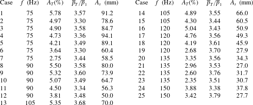
In the experiments, the frequency and amplitude of the pressure excitations are changed to estimate the effects of downstream excitations on unsteady shock train motions. Table 3 presents the pressure excitations (
 $f$
,
 $A_{T}$
,
 $\overline{p}_{T}/\overline{p}_{1}$
) and the corresponding oscillation amplitudes of the shock train
 $A_{s}$
, the oscillation amplitudes determined with the pressure ratio method have error bounds of [
 $-4$
mm,
 $+4$
mm]. As can be seen, the excited frequency is controlled exactly in the test cases, and the amplitude of the imposed pressure variation and the mean pressure value are real measurements. The experimental cases shown in table 3 are grouped by the excited frequency. In all test cases, the parameter
 $k_{1}$
is equal to 0.07312 which is calculated at the inlet of the duct,
 $\overline{M}_{1}$
is the Mach number of the incoming flow and
 $\overline{a}_{1}$
equals
 $253.55~\text{m}~\text{s}^{-1}$
and is evaluated from the undisturbed flow.
The experimental results.

According to (4.21), the forced shock train movement includes a decay motion
 $A_{1}(e^{-Pt}/\sqrt{p^{2}/w^{2}+1})$
. As can be seen, the decay motion has larger effects on the amplitude of the periodical motion
 $A_{1}$
when the excited frequency
 $w$
is higher. From table 3, the highest frequency excited downstream is 150 Hz. Taking case 25 (
 $w=942$
) for example, the decay motion has only a 0.46 % effect on the sinusoidal amplitude
 $A_{1}$
after 20.0 ms (3 times the period
 $1/f=1/150$
), and this quickly decreases to 0.08 % after 26.7 ms (4 times the period
 $1/f=1/150$
). In each test case, it usually takes several seconds for the excitation system (see figure 1) to work steadily, and measurements are taken after that. That is to say, the decay motion has almost no effect on the sinusoidal motion during our measurements. Therefore, the sinusoidal amplitude can be used to predict the shock train amplitude
 $A_{s}=2A_{1}$
. Substituting P and Q to calculate the amplitude
 $A_{s}$
, the theoretical prediction for shock train amplitude is:
 $$\begin{eqnarray}A_{s}=\frac{2k_{1}A_{T}\displaystyle \frac{\overline{p}_{T}}{\overline{p}_{1}}\left(6.8\displaystyle \frac{\overline{p}_{T}}{\overline{p}_{1}}-5.8\right)}{\sqrt{(\overline{M}_{1}^{2}-1)^{2}+\left(\displaystyle \frac{2\overline{M}_{1}\overline{x}_{s}w}{\overline{a}_{1}}\right)^{2}}}.\end{eqnarray}$$
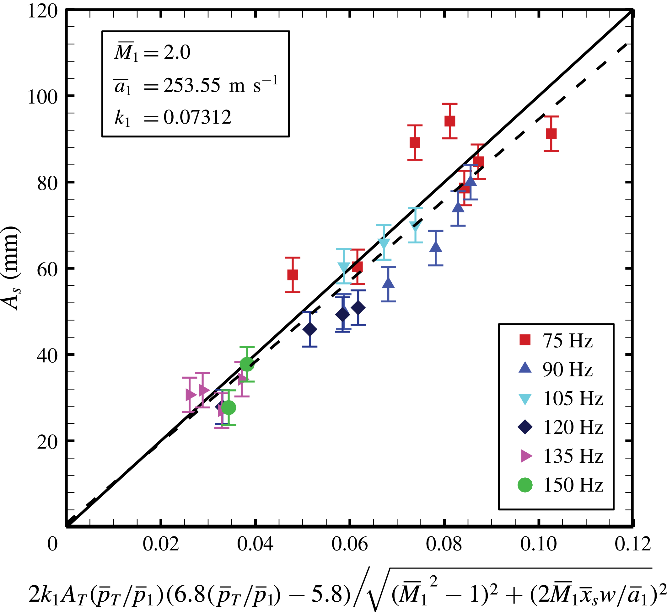
Figure 13 presents the comparison between the analytical prediction and the experimental data. The unit of the abscissa is metres and the unit of the ordinate is millimetres. For each test case shown in table 3, the experimental amplitudes of the shock train are presented in the last row
 $A_{s}$
and the analytical value can be calculated from (4.22) with the test conditions (rows 2–4 in table 3). The linear fit correlation from the experiment data is plotted as the dashed line. The expression for the fit line is
 $A_{s}=937.2C+0.883$
, where
 $C$
represents the combined parameter shown in the horizontal axis, and the goodness of fit
 $r^{2}$
is 0.879. The analytical slope of the predicted line is 1000, which is 6.70 % larger than the experimental fit line.
Comparison of analytical results and experimental results. The values of incoming flow parameters are shown in this figure.

For each case, the relative error of the predicted oscillation amplitude is defined quantitatively as:
 $$\begin{eqnarray}e_{As}=\frac{A_{sp}-A_{se}}{A_{se}}\times 100\,\%,\end{eqnarray}$$
where
 $e_{As}$
is the relative error,
 $A_{sp}$
is the predicted amplitude calculated from (4.22) and
 $A_{se}$
is the experimental amplitude. The distributions of absolute error
 $(A_{sp}-A_{se})$
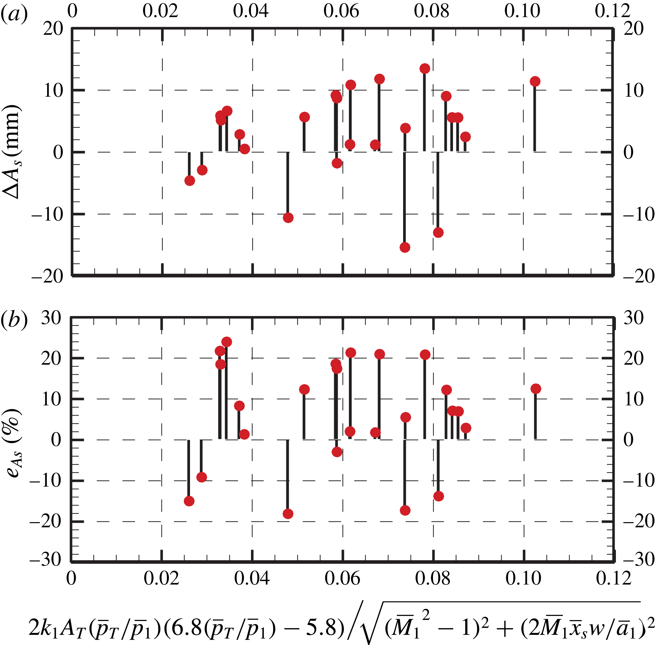
and relative error are both presented in figure 14.
From figure 14, the range of absolute error is [
 $-$
15 mm, 14 mm] and the range of relative error is [
 $-$
18 %, 23 %]. The maximum relative error occurs in case 25, and the corresponding absolute deviation is 6.7 mm. The absolute deviation is small in some cases, however, the relative error could be very large because the absolute oscillation amplitude is small (as in case 25). In addition, the predicted oscillation amplitude is larger than the experimental value in most cases. This implies that the analytical correlation equation (4.17) has an inherent positive deviation compared to the experimental value, which can also be found in figure 13, and the reason will be discussed in the following.
The distributions of absolute error (a) and relative error (b).

As can be seen, the agreement between the predicted amplitudes and experimental values is good, and the total trend of correlation between oscillation amplitude and several flow parameters can be predicted using (4.22). This significantly suggests that the analytical model can make reasonable predictions of the complex unsteady shock train motion in a constant-area duct. Essentially, the analytical model is based on the mechanism for unsteady shock train motions, which is such that the shock train keeps moving to change the relative velocity ahead of shock train and then matches the varying imposed excitation. For modelling the unsteady shock train, the key factor, the relative Mach number ahead of shock train, is obtained to make the shock train moving velocity
 $v_{s}^{\prime }$
equivalent to the increment of the incoming flow velocity
 $u_{1}^{\prime }$
, see (4.1). Therefore, the mechanism illustrated above, especially the relative Mach number, plays a significant role in modelling the unsteady shock train motion.
4.3 Discussion
As has been mentioned above, the prediction has an inherent positive deviation from the experimental value, and the main deviation source will be estimated here. From (4.9), it is known that the downstream pressure disturbance
 $p_{e}^{\prime }$
is replaced by the pressure fluctuation measured at position T
 $p_{T}^{\prime }$
. The replacement is based on a precondition that the streamwise pressure gradient at position T is negligible, as illustrated in (4.4). It can be known from (3.1) that the longer the distance
 $x_{T}$
is, the smaller the streamwise pressure gradient at position T will be. However, the streamwise pressure gradient at position T is a positive value in our test case, because the length of the duct is not large enough. As a result, the oscillation amplitude will be predicted to be larger when replacing
 $p_{e}^{\prime }$
with
 $p_{T}^{\prime }$
. This also implies that the predicted deviation would be smaller if a more downstream position was chosen for the pressure measurements
 $p_{T}(t)$
.
The analytical correlation equation (4.22) can predict some interesting phenomena. Firstly, the correlation suggests that the oscillation amplitude of the shock train motion
 $A_{s}$
decreases with an increasing excited frequency
 $f$
. This inference could be confirmed when comparing cases 2, 10 and 16 in table 3 (or cases 5, 15 and 18), which have almost the same excited amplitude
 $A_{T}$
. Moreover, it is inferred from (4.22) that the oscillation amplitude of the shock train motion
 $A_{s}$
increases with an increasing excited amplitude
 $A_{T}$
. This could be confirmed when comparing cases 8–12 (or cases 16–19), which have the same excited frequency
 $f$
.
Actually, these two phenomena have already been found in the work of Su et al. (Reference Su, Ji and Chen2016), which studied unsteady shock train motions using computational methods. This suggests that the correlation equation (4.22) theoretically confirms the phenomena which have been found in previous research, and illustrates the correlation quantitatively.
According to (4.22), it is interesting that the oscillation amplitude of the shock train motion
 $A_{s}$
would not increase infinitely with an decreasing excited frequency
 $f$
. The oscillation amplitude would increase to a constant value when the excited frequency
 $f$
decreases to zero, and this value is:
 $$\begin{eqnarray}A_{s}=\frac{2k_{1}A_{T}\displaystyle \frac{\overline{p}_{T}}{\overline{p}_{1}}\left(6.8\displaystyle \frac{\overline{p}_{T}}{\overline{p}_{1}}-5.8\right)}{\overline{M}_{1}^{2}-1}.\end{eqnarray}$$
The physical meaning of this expression should be clarified here. When the excited frequency decreases to zero, this means that there are no excitations downstream. As a result, the oscillation amplitude
 $A_{s}$
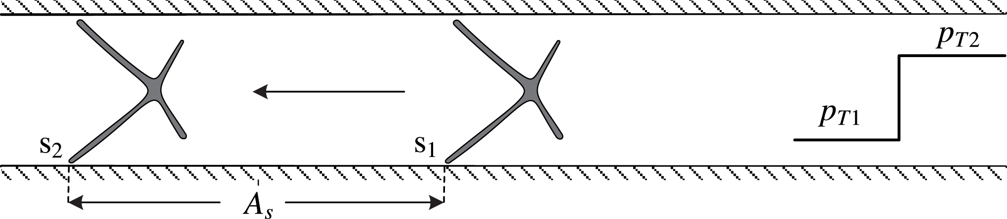
presented in (4.24) essentially gives the displacement of the shock train when subjected a pressure jump for a steady case. Figure 15 schematically presents the displacement of the shock train. For steady case 1, the downstream back pressure is
 $p_{T1}$
, and the STLE is located at position s
 $_{1}$
, corresponding to the most downstream position of the shock train motions. When subjected to a pressure jump, the downstream back pressure jumps to
 $p_{T2}$
, and the STLE is located at position s
 $_{2}$
, corresponding to the most upstream position. So, the displacement of the shock train corresponds to the oscillation amplitude of the shock train motions
 $A_{s}$
. The corresponding mean pressure ratio
 $\overline{p}_{T}/\overline{p}_{1}$
and normalized pressure amplitude
 $A_{T}$
are computed as:
 $$\begin{eqnarray}\displaystyle & \displaystyle \overline{p}_{T}=\frac{p_{T1}+p_{T2}}{2} & \displaystyle\end{eqnarray}$$
 $$\begin{eqnarray}\displaystyle & \displaystyle A_{T}=\frac{\unicode[STIX]{x0394}p_{T}}{\overline{p}_{T}}=\frac{(p_{T2}-p_{T1})/2}{(p_{T2}+p_{T1})/2}=\frac{p_{T2}-p_{T1}}{p_{T2}+p_{T1}}. & \displaystyle\end{eqnarray}$$
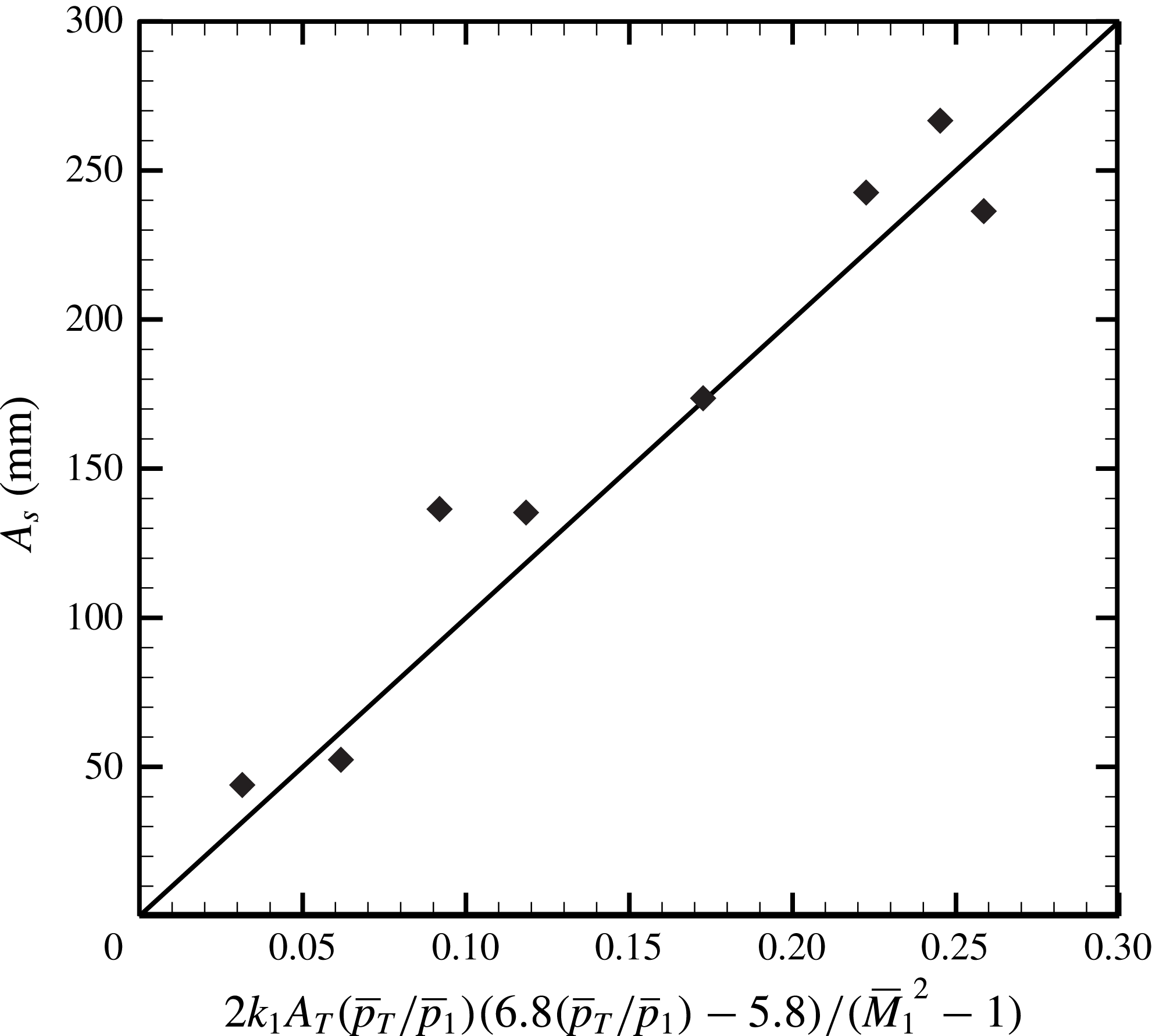
The displacement of the shock train when subjected to a downstream pressure jump for steady cases can be predicted using (4.24)–(4.26), and the steady results presented in figure 4 were used to confirm the prediction (4.24) for the steady case. Firstly, a case is chosen as the reference case (the reference case is shown in figure 4), and all displacements for the other steady cases are based on its STLE position. When subjected to several different pressure jumps, the corresponding displacements from the reference position (reference case) can be obtained. The comparison between the prediction (4.24) for the steady case and experimental results are presented in figure 16. It can be found that displacements from a reference position can be well predicted using the unsteady correlation when the excited frequency decreases to zero.
The displacement of the shock train when subjected to a downstream pressure jump.

The comparison between the prediction (4.24) for the steady case and the experimental results.

According to the above discussion, the oscillation amplitude of an unsteady shock train in a constant-area duct could be predicted just based on the information of the incoming flow and a pressure measurement point T. That is to say, if we place a pressure measurement point in the mixing region, where the streamwise pressure gradient is negligible, the oscillation amplitude of the unsteady shock train can be easily predicted. This is very useful for practical applications. The dangerous level of inlet unstart may be evaluated with this theoretical model (a large amplitude of shock train oscillation may lead to inlet unstart). In addition, it may also be used as a part of a feedback control system to prevent inlet unstart.
5 Conclusions
The response of a shock train to downstream high-frequency excitations was primarily conducted using experiments. It was found that the downstream pressure disturbance could travel in the counterflow direction through the subsonic boundary layer to induce shock train motions. As a result, a normal shock train has been observed to undergo a periodical forced oscillation in response to the downstream excitations. During the shock train movement, obvious differences between the pressure rises induced by a moving shock train and a steady shock train have been observed. For a steady case, a shock train changes its position to match a downstream pressure jump. Different from the steady cases, the mechanism by which the moving shock train responds to downstream excitations is to keep moving so that the relative Mach number ahead of the shock train changes to match the varying imposed back pressure.
Based on the ‘relative Mach number’ mechanism and a quasi-steady assumption, the unsteady shock train motion was analysed theoretically. An analytical correlation, which is a quantitative and explicit expression, between the amplitude of the shock train motion and some flow parameters was illustrated. After experimental confirmation, it is concluded that the agreement between predictions and experimental results is good, and the analytical correlation can make reasonable predictions of unsteady shock train motions in a rectangular duct. In addition, some phenomena found in previous research can be confirmed theoretically with the analytical model, for example the shock train amplitude decreases with increasing excited frequency and decreasing excited amplitude.
6 Nomenclature
-
 $\unicode[STIX]{x1D6FD}$
shock angle
-
$x$
distance from the beginning point
-
$\unicode[STIX]{x1D703}$
momentum thickness of boundary layer
-
$p$
pressure
-
$t$
time
-
$f$
frequency
-
$\unicode[STIX]{x1D70E}$
standard deviation
-
$\unicode[STIX]{x1D6FE}$
intermittent factor
-
$u$
velocity for flow
-
$w$
circular frequency
-
$e$
error
-
$M$
Mach number
-
$H$
height of duct
-
$Re$
Reynolds number
-
$k$
empirical constant
-
$T$
period
-
$L$
length
-
$N$
number of samples
-
$v$
velocity for shock train
-
$a$
sound speed
-
$A$
amplitude


Subscript
-
$l$
point or length
$l$
-
$f$
final point
-
$r$
relative value
-
$T$
point T
-
$sp$
predicted result
-
$1$
incoming flow
-
$ref$
reference value
-
$e$
excitation
-
$s$
shock train
-
$se$
experimental result


Superscript
-
$^{\prime }$
disturbance value
-
$\overline{\ast }$
value for the steady case


Acknowledgements
The authors gratefully acknowledge the support of the National Natural Science Foundation of China (grant nos 11372347 and 11572347) for this work.