1. INTRODUCTION
Although the exact density of the two-stage least squares (TSLS) estimator has been known for a few decades (see, e.g., the review by Phillips, 1983) some of its properties are still surprising for econometricians. Bimodality is one of these unexpected properties: Phillips and Wickens (1978; Sol. 6.19, pp. 351–355), Nelson and Startz (1990), Maddala and Jeong (1992), and Woglom (2001) have shown that the density of the TSLS estimator may be bimodal in a just-identified structural equation.
This paper investigates existence of bimodality in the density of the TSLS estimator in the context of a just-identified/overidentified structural equation. First, we look at the claim that the exact finite-sample distribution of the TSLS estimator cannot be easily interpreted (e.g., Woglom, 2001, p. 1381). We show that the possible bimodality of the density of the TSLS estimator can be easily understood, and generalized to overidentified models, using the exact results reviewed by Phillips (1983). In fact, it is the outcome of the interaction of two components of the exact density: one has only one mode and is symmetric around zero; the other has the shape of a pulse wave and depends on both the strength of the instruments and the degree of endogeneity. We prove a necessary condition for bimodality of the density of the TSLS estimator and show that the bimodality does not occur if the degree of overidentification is large enough.
Next, we analyze the interaction between lack of identification and high degree of endogeneity. We argue that there are an infinite number of possible densities for the TSLS estimator when the model is unidentified, depending on the path along which the quality of the instruments goes to zero. Because these limit densities do not depend on the sample size, they can all be asymptotic distributions for the TSLS estimator when the concentration parameter is local to zero as, for instance, in the weak instruments literature.
Parts of our analysis are closely related to recent work of Hillier (2006) and Phillips (2006). Hillier (2006) studies the exact properties of the TSLS estimator by rederiving the exact density using simple conditioning arguments. Hillier (2006) links bimodality to the normalization used in specifying the interest parameter in the structural equation (see also Hillier, 1990). In this paper, we are only concerned with bimodality, and we thoroughly study the interaction among noncentrality parameter, degree of endogeneity, and degree of overidentification to determine precise conditions for its existence. Phillips (2006) also studies the density of the TSLS estimator as the noncentrality parameter tends to zero in the just-identified model with a structural identity considered by Phillips and Wickens (1978, Sol. 6.19, pp. 351–355). The degree of endogeneity for his model is one, whereas, in this paper, we study the interaction between noncentrality parameter tending to zero and degree of endogeneity tending to one. Phillips (2006) develops some asymptotic theory, whereas we consider a fixed sample size only.
The rest of the paper is organized as follows. Section 2 presents the model. The properties of the exact density affecting bimodality of the TSLS estimator are considered in Section 3. Section 4 derives the limit densities as the correlation between right-hand-side endogenous variables and the instruments tends to zero. Section 5 concludes. Proofs are in the Appendix.
2. THE TWO ENDOGENOUS VARIABLES MODEL
Consider the simple instrumental variables model


t = 1,2,…,T, where yt and xt are endogenous variables, zt is a (k × 1) vector of exogenous variables, β and γ are unknown parameters of dimension (1 × 1) and (k × 1), respectively, and ut and vt are random errors. We assume that (ut,vt) are independent normal random variables with zero mean and covariance matrix

where −1 ≤ ρ ≤ 1 denotes the correlation between ut and vt (i.e., the degree of endogeneity), a parameter that affects the presence of bimodality in the density of the TSLS estimator (e.g., Maddala and Jeong, 1992; Woglom, 2001). If we apply the canonical transformations described in Theorem 3.3.1 of Phillips (1983) to the structural equation we obtain a canonical structural parameter

that is a bijective function of the degree of endogeneity (e.g., Phillips, 1983, eqns. (3.32) and (3.33)).
For the simple model we consider, the TSLS estimator of β is

where y and x are (T × 1) vectors having components yt and xt, respectively, PZ = Z(Z′Z)−1Z′, and Z is a T × k matrix having the vectors zt′ as rows. We focus on

which can be interpreted as the TSLS estimator of the structural parameter β* in the structural equation after reduction to canonical form. Hillier (2006) calls

the scaled estimation error in

. It follows from equation (4) that e = w − β*, so that the estimation error is zero (i.e.,

) if and only if w = β*. Similarly, the TSLS estimator equals β + (σu /σv)ρ, the probability limit of the ordinary least squares (OLS) estimator, if and only if w = 0. We will see later on that both β and β + (σu /σv)ρ are, in the terminology of Phillips (2006), magnetic attractors for the probability mass of the density of the TSLS estimator.
The density of w is given by equation (3.45) of Phillips (1983) as

where λ = γ′Z′Zγ/σv2 is the concentration parameter,

and 1F1(b;c; x) denotes a confluent hypergeometric function

(for details, see, e.g., Slater, 1960). In the preceding function (b)j = b(b + 1) …(b + j − 1). For b > 0 and c > 0, 1F1(b;c; x) is a monotonically increasing function of x. This property will be very useful later on. Equation (5) is the same as equation (22) of Hillier (2006), who writes λ and η for, respectively, our λ(1 + β*2) and −β*.
Equation (5) depends on β*, λ, and k only, and although it looks complicated, we will show in the next section that the shape of the density of the TSLS estimator depends on simple properties of confluent hypergeometric functions. In the just-identified model considered by Woglom (2001) (i.e., k = 1) the density of the TSLS estimator simplifies considerably (e.g., Phillips, 1980, eqn. (14); Phillips, 1983, eqn. (3.35)). Hillier (2006) gives a simple derivation of the density of both the TSLS and limited information maximum likelihood (LIML) estimators and discusses (conditional) measures of precision.
3. PROPERTIES OF THE EXACT DENSITY
The density of the TSLS estimator can be written as the product of two terms:

The first term, lt(w), usually called the “leading term” (e.g., Phillips, 1983), is obtained by replacing λ = 0 in pdf(w) and corresponds to the first line of equation (5). The second term, nc(w), is the noncentrality component and is given by the expression beginning with “exp” in equation (5). It can be written as

where Es denotes the expected value with respect to s ∼ beta((k − 1)/2,(k + 1)/2).
The bimodality of the density of the TSLS estimator is generated by the interaction between lt(w) and nc(w). Equation (7) shows that nc(w) is a monotonically increasing function of α(w), and its shape is mainly determined by α(w). If β* ≠ 0, the function α(w) has the form of a pulse wave, and as β* increases it tends to become v-shaped because the crest (highest part of the wave) becomes less noticeable.
PROPOSITION 1.
(i) lt(w) is symmetric around the origin.
(ii) If β* = 0 then nc(w) is bell-shaped, but if β* ≠ 0 then nc(w) has the form of a pulse wave; the undisturbed level (the equilibrium level as w tends to infinity) is at

the crest (highest part of the wave) is at w = β* where nc(w) equals

and the trough (lowest part of the wave) is at w = −1/β* where nc(w) takes on the value

Although the leading term tends to center the probability mass of the TSLS estimator at the probability limit of the OLS estimator, the term nc(w) tends to concentrate it around β. When one of these two terms dominates, the density of the TSLS estimator has only one relevant mode. However, when none prevails, bimodality may appear (cf. Hillier, 2006). Note that the leading term tends to shift the location of the principal mode of the density away from the correct point β (cf. Hillier, 1990).
One would expect to observe bimodality in the density of the TSLS estimator when (ncC − ncU)/(ncU − ncT) is approximately one and ncC − ncT is large, because in this case nc(w) has a deep trough and a high crest of similar size. The following results suggest situations when this may happen.
PROPOSITION 2.
(i) If either β* = 0 or λ = 0, then both nc(w) and pdf(w) are bell-shaped.
(ii) If β* ≠ 0 and λ is large, then nc(w) has a high crest (ncC − ncU = O(λ1/2)) and a shallow trough (ncU − ncT = O(1/λ)). There could be two modes in the density of w, but one of them would be very small and, certainly, undetectable for large values of the concentration parameter λ.
(iii) If λ ≠ 0 and |β*| is large, then nc(w) has a high crest (ncC − ncU = O(|β*|k2)) and a deep trough (ncU − ncT = O(|β*|k2)), so that pdf(w) could present two relevant modes (one on each side of w = 0).
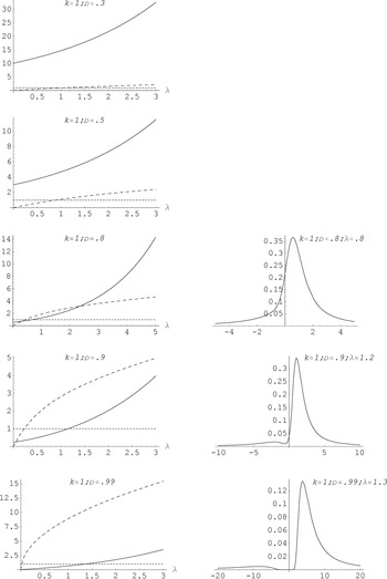
Figure 1 shows some typical shapes of (ncC − ncU)/(ncU − ncT) and ncC − ncT as functions of λ for different values of ρ and k = 1. When |ρ| is small (e.g., ρ = 0.3 and ρ = 0.5 as in the first two graphs from the top), ncC − ncU is much larger than ncU − ncT, so that there cannot be any bimodality in the density of the TSLS estimator. When ρ = 0.8, (ncC − ncU)/(ncU − ncT) ≃ 1 for λ = 0.8, but ncC − ncT is small around that point λ = 0.8, and the fluctuations of nc(w) are not large enough to generate any bimodality in the density of the TSLS estimator. For ρ = 0.9, (ncC − ncT)/(ncU − ncT) ≃ 1, and ncC − ncT is large, and bimodality appears.

Graphs of (ncC − ncU)/(ncU − ncT) (solid lines), ncC − ncT (dashed lines), and 1 (dotted lines) as functions of λ on the left-hand side and density of w on the right-hand side, for k = 1 and different values of ρ. The graphs of the densities are shown for values of λ yielding (ncC − ncU)/(ncU − ncT) ≃ 1. For ρ = 0.3 and ρ = 0.5 there are no values of λ for which (ncC − ncU)/(ncU − ncT) ≃ 1, and no density is shown on the right-hand side.
Regarding nc(w) as the only factor determining bimodality of the density of the TSLS estimator is a simplification even if it gives an intuitive explanation for bimodality. The leading term plays a very important role too, but the study of their interaction is very complicated. For example, for k > 1, the graphs of (ncC − ncU)/(ncU − ncT) and ncC − ncT show similar patterns to those in Figure 1. However, the leading term tends to concentrate around zero and to dominate so that bimodality becomes less likely.
We now give a necessary condition for the existence of bimodality in the density of the TSLS estimator.
THEOREM 1. A necessary condition for the existence of bimodality in the density of the TSLS estimator is that Δ < 0 where

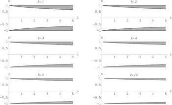
The shaded areas in the graphs in Figure 2 show the regions in the (λ,ρ) plane where the necessary condition for bimodality is satisfied for different values of k. Figure 2 makes clear that high endogeneity is a necessary, although not sufficient, condition for bimodality. Moreover, because the shaded area (where Δ < 0) shrinks as the degree of overidentification increases, bimodality becomes less likely. This is formally stated in the following corollary.

Regions in the (λ,ρ) plane where the necessary condition for the existence of bimodality is satisfied (shaded areas) for different values of k.
COROLLARY 1. If k is large, β* ≠ 0 and finite, and λ > 0, then the density of the TSLS estimator has only one mode in a neighborhood of β + (σu /σv)ρ.
Therefore, as the number of instruments becomes large, the density of the TSLS estimator tends to have only one mode in the neighborhood of β + (σu /σv)ρ. Intuitively, (1 + w2)−(k+1)/2 in the leading term lt(w) becomes concentrated around zero and dominates nc(w) when k is large (cf. Bekker, 1994; Chao and Swanson, 2005; Han and Phillips, 2006; Hillier, 2006, Prop. 5).
The exact distribution of the OLS estimator of the canonical structural parameter β* is given by equation (5) with k replaced by T (e.g., Phillips, 1983). The results of the recent analysis of Kiviet and Niemczyk (2005) about the small-sample properties of the OLS and the TSLS estimators and their relative performance can be explained using Theorem 3 in Section 4 and Proposition 1. If T is large, and k and the noncentrality parameter are small, then the OLS estimator is very concentrated around its probability limit, whereas the probability mass for the TSLS estimator may be split between β + (σu /σv)ρ and β. In this situation, the OLS estimator may perform better than the TSLS estimator in terms of mean squared error (or analogous measures if k = 1). As k increases, the difference between the densities of the OLS and the TSLS estimators vanishes (cf. Bekker, 1994; Hillier, 2006, Rmk. 8). Hillier (2006) argues that the LIML estimator is better centered than the TSLS estimator when the degree of overidentification is large because its leading term does not depend on k.
In a just-identified/overidentified structural equation, one may thus follow Woglom (2001) and conclude that “practically important bimodality [in the density of the TSLS estimator] requires high endogeneity […] along with relatively small first stage correlation” (p. 1387). As the degree of overidentification increases, bimodality becomes less likely.
4. THE MODEL WITH AN UNIDENTIFIED STRUCTURAL PARAMETER
Phillips and Wickens (1978), Nelson and Startz (1990), and Phillips (2006) consider a model with k = 1 consisting of a structural equation like the one in equation (1) and a structural identity (i.e., xt = yt + ztγ instead of equation (2)) with degree of exogeneity equal to one. They conclude that bimodality is always a feature of the exact density of the TSLS estimator. The model used in this paper, specified in equations (1) and (2), does not contain any structural identity, and it is not directly comparable to that of Phillips and Wickens (1978), Nelson and Startz (1990), and Phillips (2006). However, it can be used to illustrate the effects of strong endogeneity on the exact density of the TSLS estimator when the model is close to being unidentified. The differences between the models with and without a structural identity are discussed by Phillips (2006).
The partial Fisher information for β is λσv2/σu2, and it tends to zero as λ → 0. In this case the noncentrality term vanishes (e.g., Phillips, 1983), unless the effect of λ → 0 is canceled out by the degree of endogeneity ρ2 going to one (or, equivalently, β*2 → ∞). We will study these limits along a path of the form λ = θ(1 − ρ2) + o(1 − ρ2), 0 ≤ θ < ∞. In this case w is not defined but the limiting density of the TSLS estimator is. In the notation of Section 2.4 of Hillier (2006), the direction φ tends to (0,±1)′ when β*2 → ∞, and these are points where the coordinates

are not defined.
If θ = 0, the TSLS estimator has a Cauchy distribution for any |ρ| < 1 (e.g., Phillips, 1983). If θ > 0, the situation is more complicated, and the following theorems give some insights about the shape of the limit density.
THEOREM 2. Suppose λ → 0 and ρ2 → 1 on the path λ = θ(1 − ρ2) + o(1 − ρ2), 0 ≤ ∞ < ∞; then
(i) the density of the TSLS estimator is

(ii) If the model is just identified (k = 1) then the limit of the density simplifies to

THEOREM 3. The limit density in Theorem 1 has the following properties:
(i) if k = 1 bimodality occurs for θ > 1;
(ii) if k = 2 then bimodality occurs for θ > 3.15991;
(iii) if k ≥ 3 the density is always unimodal.
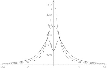
Figure 3 shows the limit density in the just-identified case for some values of parameter θ. Theorem 3 suggests that if the model is unidentified (or close to being unidentified) and the number of instruments is large then the distribution of the TSLS estimator is also concentrated around β + (σu /σv)ρ. This result holds true independently of the path chosen to calculate the limit density. Moreover, because the exact density given in Theorem 1 does not depend on the sample size, it is also the asymptotic density for the TSLS estimator.

Graphs of the limit densities of w in the just-identified case for θ = 0 (dashed line), θ = 1 (dotted line), and θ = 3 (solid line).
For k ≤ 2, if the value of θ is sufficiently large that λ is larger than 1 − ρ2, bimodality arises because the TSLS estimator is simultaneously attracted toward the values of ±β and β + (σu /σv)ρ. Phillips (2006) provides an asymptotic expansion for the position of the modes in the just-identified case that captures the criterion in Theorem 3(i). If k ≥ 3, then there is no bimodality because the attraction toward the probability limit of the OLS estimator prevails.
5. CONCLUSIONS
Phillips and Wickens (1978), Nelson and Startz (1990), Maddala and Jeong (1992), and Woglom (2001) have shown that the density of the TSLS estimator may be bimodal in a just-identified structural equation. This paper has looked further at this issue in a just-identified/overidentified structural equation to provide a better understanding of the problem.
Our conclusions are as follows.
- Bimodality arises because of the complex interaction between two components of the exact density: one of these is symmetric, and one has the shape of a pulse wave. Depending on the value of three key parameters, the noncentrality parameter, the degree of endogeneity, and the degree of overidentification, we may or may not observe bimodality in the density of the TSLS estimator.
- As for the just-identified case, bimodality occurs if the noncentrality parameter is large. However, one of the modes surely would be undetectable in this case. Clear bimodality tends to occur when the degree of endogeneity is close to one and the noncentrality parameter is relatively small.
- The limit density of the TSLS estimator as the noncentrality parameter tends to zero and the degree of endogeneity tends to one may have one or two modes when the degree of overidentification is less than or equal to two. In all other cases it has only one mode centered around the probability limit of the OLS estimator.
- When the noncentrality parameter is finite, bimodality in the density of the TSLS estimator becomes less likely as the degree of overidentification increases (in this case the density has only one mode in the neighborhood of the probability limit of the OLS estimator).
TECHNICAL APPENDIX
Proof of Proposition 1. Equations (9) and (10) can be easily obtained from the expression beginning with “exp” in equation (5). Equation (8) follows easily from (7) after taking the limit as w tends to infinity. █
Proof of Proposition 2. These results follow from Proposition 1 and approximations for the confluent hypergeometric function reviewed by Slater (1960). █
Proof of Theorem 1. Bimodality exists when

has at least three real solutions in w. The last equation can be rewritten as

It can be easily checked that −(dlt(w)/dw)/lt(w) = (1 + k)w/(1 + w2). From (7) we find that

This is a continuous function of w; moreover, because for every q ≥ 0 we have 1F1(k; k/2;q) ≥ 1F1(k + 1; k/2 + 1;q), and 1 − s ≤ 1, the ratio of the two expectations in the preceding display is always between zero and one, so that the right-hand side of equation (A.1), as a function of w, is always between the horizontal axis and the function

Therefore, a necessary but not sufficient condition for the existence of bimodality is that

has at least three real solutions. Simplifying and rearranging the last equation, we conclude that a necessary condition for the existence of bimodality is that the cubic equation

has three real solutions. The theorem follows from standard results on the number of real solutions of cubic equations. █
Proof of Corollary 1. We have seen in the proof of Theorem 1 that a necessary condition for the existence of bimodality is that

As k → ∞ the left-hand side increases, but the right-hand side stays the same for fixed β and λ. If k is large enough the preceding equation will have only one real solution between min{β*,−1/β*} and max{β*,−1/β*}. The slope of (1 + k)w tends to infinity as k → ∞, so that (1 + k)w tends to a vertical line going though the origin and intersects the curve representing the right-hand side of equation (A.2) in a neighborhood of zero only. █
Proof of Theorem 2. Using (5) we can write λ = θ/(1 + β*2) + o((β*)−2), and the statement of the theorem follows easily from the continuity of the exponential and of the hypergeometric functions.
Proof of Theorem 3. It is easily verified that the limit density can have only two modes and that if a trough exists it must occur at w = 0. Moreover, one can easily show that

so that
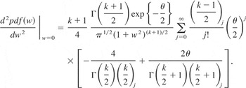
After using equation (2.2.4) of Slater (1960) and simplifying, one obtains

and d2pdf(w)/dw2|w=0 > 0 if and only if 1F1((k − 3)/2; k/2;θ/2) < 0. For k = 1 one has 1F1(−1;½;θ/2) = 1 − θ < 0, which implies θ > 1. For k = 2, 1F1(−½;1;θ/2) < 0, which implies θ > 3.15991. For k ≥ 3, 1F1((k − 3)/2; k/2;θ/2) ≥ 1 for all θ so that d2pdf(w)/dw2|w=0 ≤ 0 for all θ.