1 Introduction
At high speeds, the laminar–turbulent transition has a significant impact on heating loads over hypersonic vehicles. The hypersonic flights require improved understanding of the laminar–turbulent transition in a complex three-dimensional body. In general, the combination of three-dimensional geometry and pressure gradient can result in curved inviscid streamlines at the boundary layer edge. Then the resulting three-dimensional boundary layer profiles, which are highly inflectional, can lead to the cross-flow instability (Gray Reference Gray1952). Cross-flow disturbances may be either stationary or travelling, and travelling cross-flow modes will be excited inside of the three-dimensional boundary layer by the free-stream turbulence, while stationary modes are highly receptive to the surface roughness near the leading edge (Bippes Reference Bippes1999). Travelling cross-flow modes are more unstable than stationary cross-flow modes according to linear stability theory (LST). Stationary cross-flow vortices can be excited in the three-dimensional boundary layers, and then develop secondary instabilities. A number of research studies have been conducted on the secondary instabilities of stationary cross-flow vortices at low speed, as the flight environment was expected to be quiet (Saric, Reed & White Reference Saric, Reed and White2003). In an experiment, Poll (Reference Poll1985) found that high-frequency disturbances were induced by the cross-flow secondary instability. Kohama, Saric & Hoos (Reference Kohama, Saric and Hoos1991), Kohama, Onodera & Egami (Reference Kohama, Onodera and Egami1996) showed that the onset of high-frequency disturbance was caused by multiple inflection points, indicating the onset of the laminar–turbulent transition. Malik et al. (Reference Malik, Li, Choudhari and Chang1999) introduced two categories for the secondary cross-flow instability modes: high-frequency mode ‘z’, produced by the minimum of the spanwise gradient of the streamwise velocity; high-frequency mode ‘y’, produced by the maximum of the wall-normal gradient of the streamwise velocity. White & Saric (Reference White and Saric2005) experimentally confirmed that the breakdown of cross-flow vortices was always observed downstream of the onset of high-frequency secondary instabilities. An emphasis was placed upon the ‘z’ mode, as it was more likely excited in experiments rather than the ‘y’ mode, and the reason for this is currently unclear. Furthermore, it was both numerically and experimentally shown (White & Saric Reference White and Saric2005; Li & Choudhari Reference Li and Choudhari2011) that the low-frequency mode originated from travelling cross-flow waves in the upstream region, where the boundary layer flow was almost not disturbed. Thereby, the low-frequency mode was often referred to as a ’modulated travelling wave’ (Li & Choudhari Reference Li and Choudhari2011).
A number of research studies have been conducted on the receptivity and stability characteristics in high-speed three-dimensional boundary layer flows. For the flow over a yawed cone in a hypersonic state, the cross-flow-dominated transition was detected, and Stetson et al. (Reference Stetson, Thompson, Donaldson and Siler1984) found that stationary cross-flow vortices were also sensitive to the wall roughness. Balakumar & Owens (Reference Balakumar and Owens2010) using both direct numerical simulation (DNS) and linear stability theory investigated the cross-flow instability inside a Mach 6.0 boundary layer on a
 $7^{\circ }$
half-angle cone at
 $6^{\circ }$
of angle of attack. The DNS results confirmed that stationary disturbances can be directly excited by the surface roughness near the tip of the cone and propagated towards the leeward region. Furthermore, the receptivity mechanism to the surface roughness in a three-dimensional boundary layer over a Mach 3.0 infinite swept wing was investigated by Balakumar & King (Reference Balakumar and King2011) using DNS. It was numerically shown that stationary vortices can be effectively generated by
 $1~\unicode[STIX]{x03BC}\text{m}$
roughness elements close to the leading-edge region. Schuele, Corke & Matlis (Reference Schuele, Corke and Matlis2013) experimentally investigated the receptivity of stationary cross-flow modes to patterned roughness in the boundary layer over a right-circular cone at Mach 3.5, and it was found that the growth rate of the stationary cross-flow mode can also be enhanced by the critical patterned roughness. Dinzl & Candler (Reference Dinzl and Candler2017) using DNS studied the evolution of stationary cross-flow disturbances over a Mach 6.0 elliptic cone. Surface roughnesses were placed on the surface of the elliptic cone to excite cross-flow disturbances. A stationary cross-flow vortex was observed in the nonlinear region, inducing a significant increase in the wall heat flux. Furthermore, Dinzl & Candler (Reference Dinzl and Candler2017) found that the spanwise wavelength of the dominant stationary cross-flow vortex was sensitive to the free-stream Reynolds number rather than the wall roughness patterns. As a consequence, it can be concluded that the stationary cross-flow mode can be effectively favoured by the surface roughness, as in incompressible swept wing flows.
In order to shed light on the mechanisms of laminar–turbulent transition in hypersonic three-dimensional boundary layer flow, the surface heat transfer and disturbance frequency on an inclined cone was measured by Ward, Henderson & Schneider (Reference Ward, Henderson and Schneider2015) in the Boeing/AFOSR Mach 6 quiet tunnel. The experiments were conducted at
 $4^{\circ }{-}6^{\circ }$
angle of attack with the surface temperature
 $T_{w}=298.1~\text{K}$
. Stationary vortex streaks originating from a ring of surface roughness near the upstream of the cone can be observed as hot streaks, and disturbances with a frequency higher than that of travelling cross-flow waves were also detected with sensors. Ward et al. (Reference Ward, Henderson and Schneider2015) suggested that these high-frequency fluctuations may be the secondary instability modes of stationary cross-flow vortices, since the high-frequency fluctuations can only be measured near the laminar–turbulent transition region. In the Mach 6 Quiet Tunnel at Texas A&M, Craig & Saric (Reference Craig and Saric2015, Reference Craig and Saric2016) studied the cross-flow instability and transition inside the boundary layer over a inclined cone at
 $5.6^{\circ }$
angle of attack. The stationary cross-flow vortex can also be observed by measuring the spatial distribution of mass flux, and the secondary instability mode ‘z’ was likely to dominate the instability dynamics. Craig & Saric (Reference Craig and Saric2015, Reference Craig and Saric2016) found that the streamwise region of instability mode ‘z’ was at least an order of magnitude longer than that of the ‘z’ mode in incompressible swept wing flow. However, no laminar–turbulent transition occurred in the experiment. Moyes et al. (Reference Moyes, Paredes, Kocian and Reed2016, Reference Moyes, Paredes, Kocian and Reed2017) numerically investigated the secondary instabilities of stationary cross-flow vortices on a hypersonic yawed cone at
 $6^{\circ }$
angle of attack; the model length and parameters were almost identical to those used by Ward et al. (Reference Ward, Henderson and Schneider2015). The three-dimensional boundary layer flow along some vortex trajectory was adopted as the base flow, and the stationary cross-flow vortex was obtained by solving the nonlinear parabolized stability equations (NPSE). A number of unstable modes, including the travelling cross-flow waves, modes ‘z’ and ‘y’ and the Mack mode, were revealed through the two-dimensional spatial bi-global analysis. Furthermore, it was found that the ‘z’ and ‘y’ modes were always located at the updraft side and on top of the stationary cross-flow vortex, respectively. Therefore, Moyes et al. (Reference Moyes, Paredes, Kocian and Reed2016, Reference Moyes, Paredes, Kocian and Reed2017) suggested that there is no intrinsic discrepancy between the secondary cross-flow instability in the hypersonic flow and that in incompressible three-dimensional boundary layers. Li et al. (Reference Li, Choudhari, Paredes and Duan2016), Choudhari et al. (Reference Choudhari, Li, Paredes and Duan2017) investigated the high-frequency secondary instabilities of stationary cross-flow vortex inside the boundary layer flow over a
 $7^{\circ }$
half-angle circular cone at Mach 6.0. The cone was pitched at
 $6^{\circ }$
angle of attack, the free-stream Reynolds number was
 $10.09\times 10^{6}~\text{m}^{-1}$
and the surface temperature of the model 300 K. Azimuthally distributed roughness elements near the tip of the cone were used to excite the cross-flow disturbances, and the evolution of stationary cross-flow modes was obtained through DNS. A high-frequency ‘z’ mode was also found according to both instability analyses and DNS results, and the behaviours of all secondary instability modes were basically consistent with low-speed cases. Furthermore, Li et al. (Reference Li, Choudhari, Paredes and Duan2016) had shown that the Mack mode originating from the unperturbed laminar flow will be modified and significantly enhanced by the finite amplitude of the stationary cross-flow vortex. The frequencies of the secondary instability mode of the stationary cross-flow vortex and that of the Mack mode were comparable, and the importance of the Mack mode in a hypersonic three-dimensional boundary layer was emphasized.
In the present work, the role played by compressibility in the secondary cross-flow instability in a hypersonic three-dimensional boundary layer flow is further studied. Nevertheless, as Li et al. (Reference Li, Choudhari, Paredes and Duan2016) pointed out that the basic flow over a pitched cone was not strictly periodic along the azimuthally spanwise direction, a rigorous formulation of secondary instability analysis could not be employed. Therefore, a three-dimensional boundary layer flow over an infinite swept wing at Mach 6.0 is adopted herein as a basic flow to maintain the mathematics at a reasonable level. In fact, the boundary layer flow over an infinite swept wing at Mach 8.15 was also used in Mack & Schmid (Reference Mack and Schmid2011) as a basic state to study the global temporal stability. In § 2, calculation of the laminar base flow is introduced. The mathematical formulation and numerical methods of the stability analysis are provided in § 3. The secondary instability analysis is presented and discussed in § 4. The present study is concluded with § 5.
2 Laminar flow
The three-dimensional laminar flow over a hypersonic swept wing is considered herein, and the swept wing is modelled by a swept parabolic body as in Mack & Schmid (Reference Mack and Schmid2011),
 $$\begin{eqnarray}\displaystyle x^{\ast }=\frac{(y^{\ast })^{2}}{2R^{\ast }}\quad \text{and}\quad R^{\ast }=0.01~\text{m}, & & \displaystyle\end{eqnarray}$$
where
 $R^{\ast }$
represents the radius of the leading edge. A local Cartesian coordinate system (
 $x^{\ast }$
,
 $y^{\ast }$
and
 $z^{\ast }$
) is used to describe the swept wing model, and a body fitted orthogonal coordinate system (
 $\unicode[STIX]{x1D709}^{\ast }$
,
 $\unicode[STIX]{x1D702}^{\ast }$
and
 $z^{\ast }$
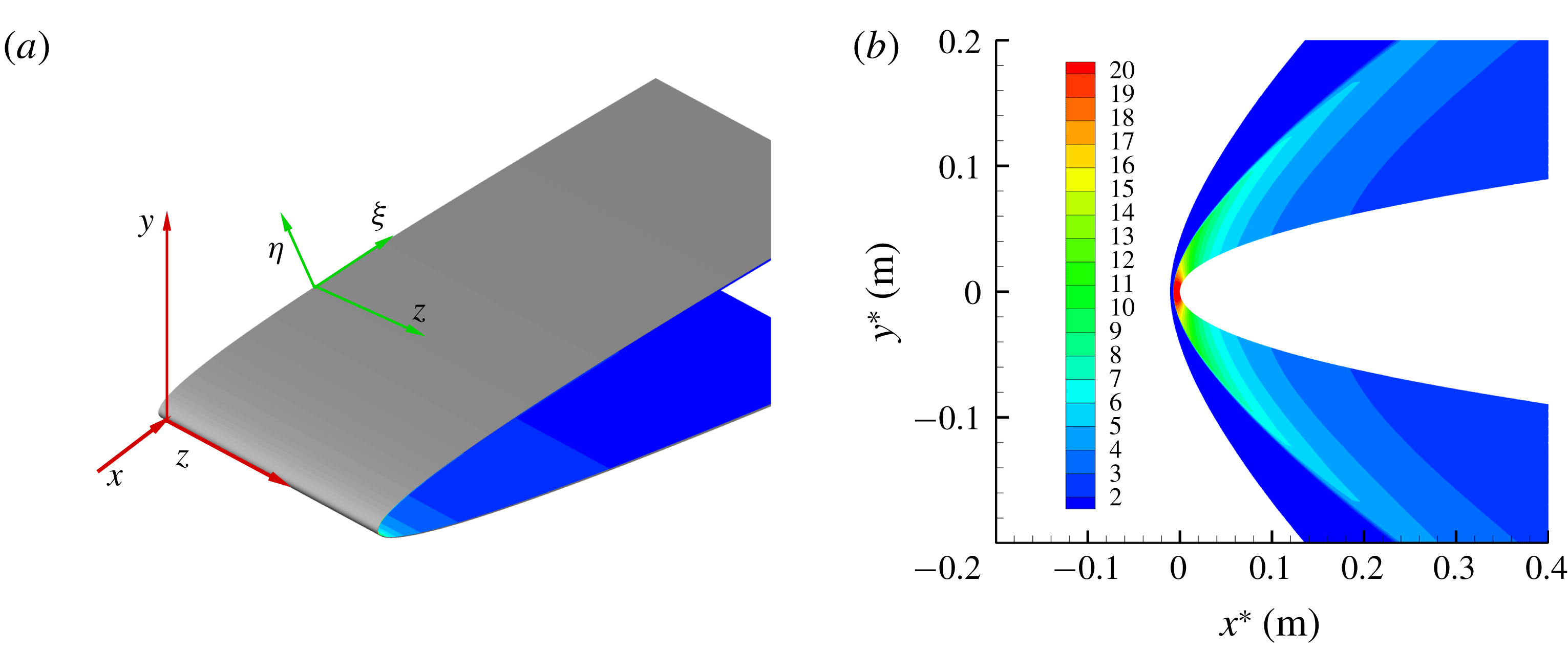
) is also defined for the flow stability analysis (figure 1(a)). Simulation conditions are shown in table 1. Here, the symbol ’
 $\ast$
’ denotes the dimensional variables, ’
 $\infty$
’ the free stream;
 $L^{\ast }$
represents the chord length and
 $\unicode[STIX]{x1D703}$
stands for the swept angle. The free-stream Mach number is 6.0 with the free-stream temperature being 57 K, and the free-stream Reynolds number
 $Re_{1}$
is
 $8.0\times 10^{6}$
, which is consistent with Borg, Kimmel & Stanfield’s (Reference Borg, Kimmel and Stanfield2015) experiment condition. No-slip and adiabatic temperature conditions are specified at the wall.
(a) The coordinate systems over the swept wing; (b) the non-dimensional pressure field of the laminar flow.

Simulation conditions.

Our well-validated in-house code is used to solve the laminar flow governed by the unsteady, compressible Navier–Stokes equations (Xu, Jiang & Liu Reference Xu, Jiang and Liu2016; Xu et al.
Reference Xu, Liu, Jiang and Qian2018b
). For the laminar flow calculation based on DNS in the present study, the free-stream density, velocity, temperature and molecular viscosity
 $\unicode[STIX]{x1D707}_{\infty }^{\ast }$
are used to scale the corresponding flow variables. A fifth-order-accurate scheme is used to treat the convective fluxes, while the diffusive fluxes are discretized using a fourth-order centred scheme. Furthermore, the solution of time integration is based on a third-order total-variation-diminishing (TVD) Runge–Kutta scheme. An ideal gas is assumed for the flow fluid, the Prandtl number
 $Pr$
is assumed to be constant and the heat flux obeys the Fourier law. The viscosity
 $\unicode[STIX]{x1D707}^{\ast }$
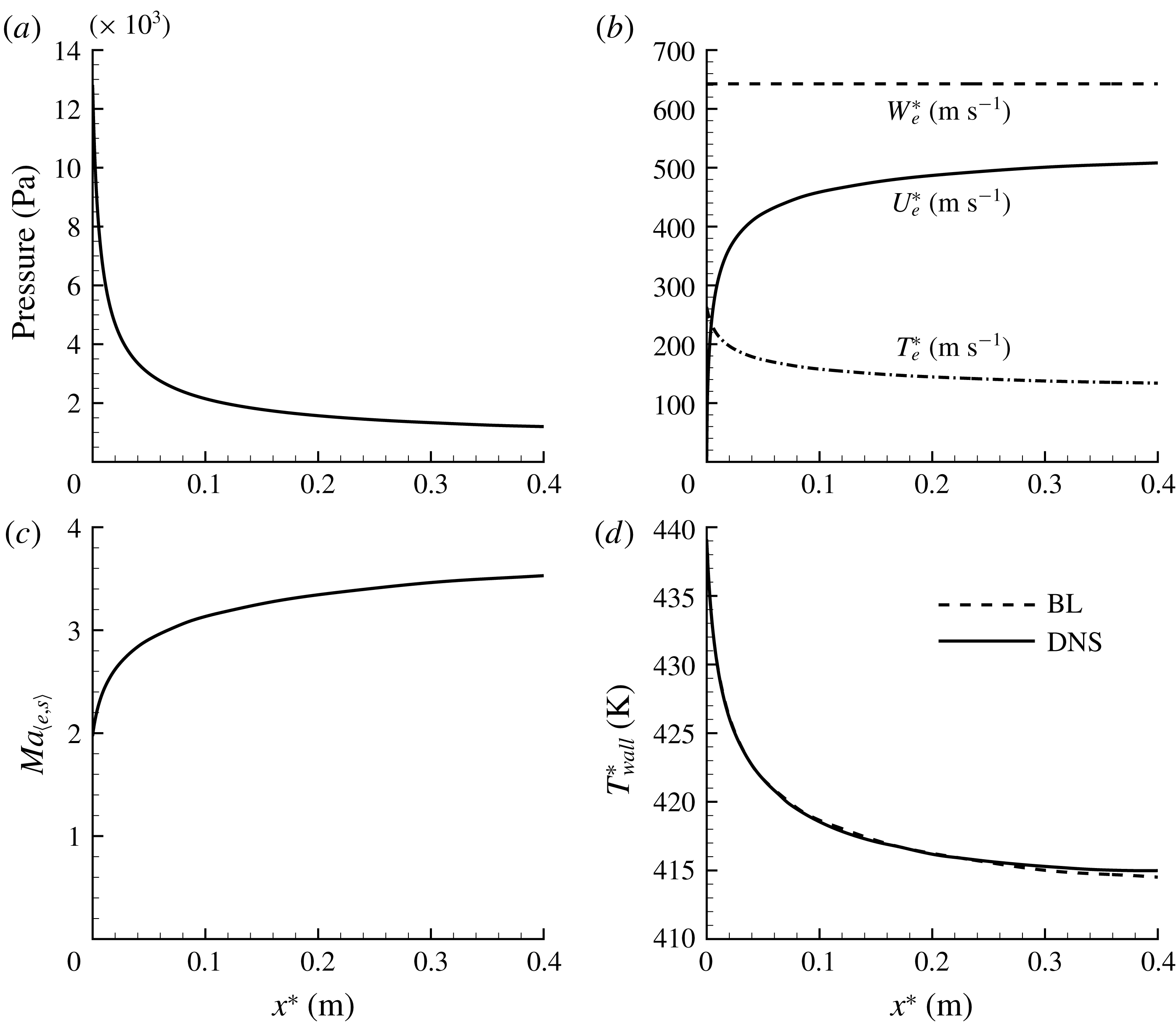
is computed using Sutherlands viscosity model. Figure 1(b) shows the spatial distribution of the pressure of the basic flow from DNS, it is seen that the bow shock can be clearly captured. Figure 2(a) shows the distribution of pressure on the wall. Figure 2(b,c) shows the distributions of velocity and temperature at the boundary layer edge, respectively (the subscript ‘e’ represents the boundary layer edge, and the temperature at boundary edge can be obtained through isentropic relations).
Evolution of the laminar flow: (a) distribution of pressure on the wall; (b) chordwise velocity, spanwise velocity and temperature at the boundary layer edge; (c) Mach number at the boundary layer edge; (d) temperature at the wall. BL, boundary layer.

Meanwhile, quasi-three-dimensional compressible boundary layer equations are also used to resolve the laminar flow (Pruett & Streett Reference Pruett and Streett1991; Xu et al.
Reference Xu, Liu, Chen and Fu2018a
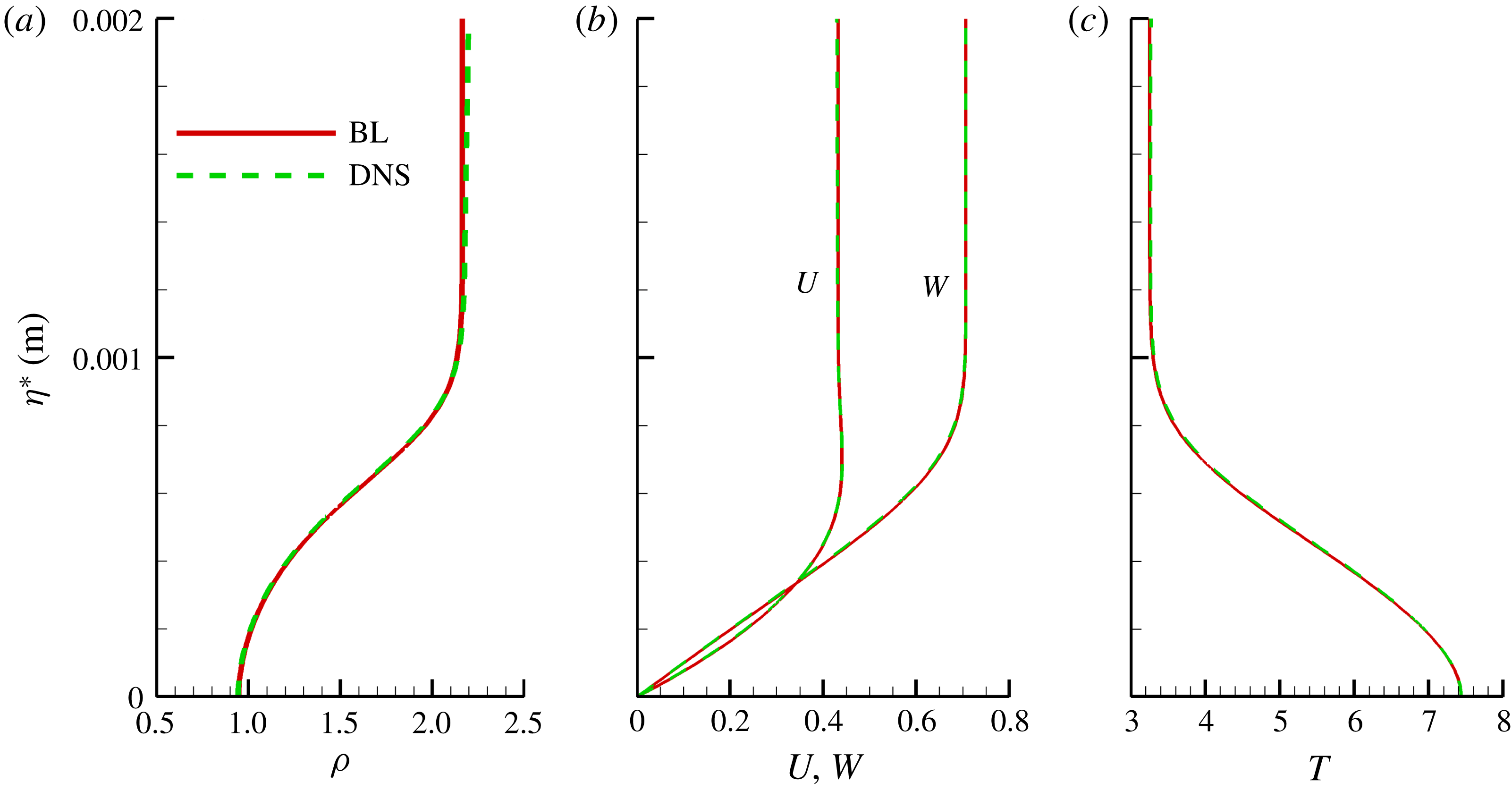
). The boundary layer equations are discretized using a spectrally accurate differencing in the wall-normal direction, a uniform grid and a fifth-order backward difference scheme is employed to discretize the streamwise direction. Figure 2(d) shows the distributions of wall temperature on the wall based on the boundary layer code and DNS. Moreover, the profiles of density, velocity and temperature at
 $x^{\ast }=0.04~\text{m}$
are also provided in figure 3. It can be seen that a good agreement between the results from the boundary layer code and DNS has been achieved.
Profiles of density, velocity and temperature based on boundary layer equations and DNS at
 $x^{\ast }=0.04~\text{m}$
.

3 Stability analysis methodology
For the flow over the infinite swept wing, a body fitted orthogonal coordinate system is also adopted for the stability analysis where
 $\unicode[STIX]{x1D709}$
,
 $\unicode[STIX]{x1D702}$
and
 $z$
denote chordwise, wall-normal and spanwise directions, respectively, as shown in figure 1(a). The flow variables are conveniently decomposed into the base (undisturbed) flow
 $Q=(\unicode[STIX]{x1D70C},U,V,W,T)$
and the disturbance quantity
 $\unicode[STIX]{x1D753}=(\unicode[STIX]{x1D70C}^{\prime },u^{\prime },\unicode[STIX]{x1D710}^{\prime },w^{\prime },T^{\prime })$
. The similarity boundary thickness
 $\unicode[STIX]{x1D6FF}_{0}^{\ast }$
, defined as
 $$\begin{eqnarray}\displaystyle \unicode[STIX]{x1D6FF}_{0}^{\ast }=\sqrt{\unicode[STIX]{x1D707}_{\infty }^{\ast }x_{0}^{\ast }/\unicode[STIX]{x1D70C}_{\infty }^{\ast }Q_{\infty }^{\ast }} & & \displaystyle\end{eqnarray}$$
at
 $x_{0}^{\ast }=0.04~\text{m}$
, is used as the length scale. According to stability theory (Herbert Reference Herbert1997), the dimensionless governing equations of the disturbance quantities can be obtained as follows:
 $$\begin{eqnarray}\displaystyle & & \displaystyle \unicode[STIX]{x1D6E4}\frac{\unicode[STIX]{x2202}\unicode[STIX]{x1D753}}{\unicode[STIX]{x2202}t}+A\frac{\unicode[STIX]{x2202}\unicode[STIX]{x1D753}}{\unicode[STIX]{x2202}\unicode[STIX]{x1D709}}+B\frac{\unicode[STIX]{x2202}\unicode[STIX]{x1D753}}{\unicode[STIX]{x2202}\unicode[STIX]{x1D702}}+C\frac{\unicode[STIX]{x2202}\unicode[STIX]{x1D753}}{\unicode[STIX]{x2202}z}+D\unicode[STIX]{x1D753}\nonumber\\ \displaystyle & & \displaystyle \quad =H_{\unicode[STIX]{x1D709}\unicode[STIX]{x1D709}}\frac{\unicode[STIX]{x2202}^{2}\unicode[STIX]{x1D753}}{\unicode[STIX]{x2202}\unicode[STIX]{x1D709}^{2}}+H_{\unicode[STIX]{x1D709}\unicode[STIX]{x1D702}}\frac{\unicode[STIX]{x2202}^{2}\unicode[STIX]{x1D753}}{\unicode[STIX]{x2202}\unicode[STIX]{x1D709}\unicode[STIX]{x2202}\unicode[STIX]{x1D702}}+H_{\unicode[STIX]{x1D709}z}\frac{\unicode[STIX]{x2202}^{2}\unicode[STIX]{x1D753}}{\unicode[STIX]{x2202}\unicode[STIX]{x1D709}\unicode[STIX]{x2202}z}+H_{\unicode[STIX]{x1D702}\unicode[STIX]{x1D702}}\frac{\unicode[STIX]{x2202}^{2}\unicode[STIX]{x1D753}}{\unicode[STIX]{x2202}\unicode[STIX]{x1D702}^{2}}+H_{\unicode[STIX]{x1D702}z}\frac{\unicode[STIX]{x2202}^{2}\unicode[STIX]{x1D753}}{\unicode[STIX]{x2202}\unicode[STIX]{x1D702}\unicode[STIX]{x2202}z}+H_{zz}\frac{\unicode[STIX]{x2202}^{2}\unicode[STIX]{x1D753}}{\unicode[STIX]{x2202}z^{2}}+f_{nonlinear}.\nonumber\\ \displaystyle & & \displaystyle\end{eqnarray}$$
3.1 Linear stability solution
The spatial development of small amplitude disturbances developing in boundary layers can be described by the linearized Navier–Stokes equations. According to linear stability theory, disturbance variables can be written as the modal expansion,
 $$\begin{eqnarray}\displaystyle \left.\begin{array}{@{}c@{}}\unicode[STIX]{x1D753}(\unicode[STIX]{x1D709},\unicode[STIX]{x1D702},z,t)=\widehat{\unicode[STIX]{x1D711}}(\unicode[STIX]{x1D702})\exp [\text{i}(\unicode[STIX]{x1D6FC}\unicode[STIX]{x1D709}+\unicode[STIX]{x1D6FD}z-\unicode[STIX]{x1D714}t)]+\text{c.c.}\\ \widehat{\unicode[STIX]{x1D711}}(\unicode[STIX]{x1D702})=(\widehat{\unicode[STIX]{x1D70C}},\widehat{u},\widehat{\unicode[STIX]{x1D710}},\widehat{w},\widehat{T}),\end{array}\right\} & & \displaystyle\end{eqnarray}$$
where
 $\widehat{\unicode[STIX]{x1D711}}$
represents the shape function of the disturbance,
 $\unicode[STIX]{x1D714}$
denotes the dimensionless disturbance frequency. For the flow over the infinite swept wing, no growth is assumed to occur in the spanwise direction, the spanwise wavenumber
 $\unicode[STIX]{x1D6FD}$
is a real number. Here,
 $$\begin{eqnarray}\displaystyle \unicode[STIX]{x1D6FD}=2\unicode[STIX]{x03C0}\unicode[STIX]{x1D6FF}_{0}^{\ast }/\unicode[STIX]{x1D706}^{\ast }, & & \displaystyle\end{eqnarray}$$
where
 $\unicode[STIX]{x1D706}^{\ast }$
stands for the spanwise wavelength. Furthermore, a spatial linear stability analysis is performed for stationary cross-flow modes, then
 $\unicode[STIX]{x1D6FC}$
is a complex variable,
 $$\begin{eqnarray}\displaystyle \unicode[STIX]{x1D6FC}=\unicode[STIX]{x1D6FC}_{r}+\text{i}\unicode[STIX]{x1D6FC}_{i}, & & \displaystyle\end{eqnarray}$$
the real part
 $\unicode[STIX]{x1D6FC}_{r}$
of which represents the streamwise wavenumber, and its imaginary part
 $\unicode[STIX]{x1D6FC}_{i}$
stands for the growth rate.
The eigenvalue problem for LST can be recovered by substituting (3.3) into the governing equation (3.2), neglecting the nonlinear term
 $f_{nonlinear}$
and the mean wall-normal velocity component. The resulting eigenvalue problem is discretized with the fourth-order central differencing scheme in the wall-normal direction, more details can be found in Xu, Xiao & Fu (Reference Xu, Xiao and Fu2011), Xu et al. (Reference Xu, Liu, Chen and Fu2018a
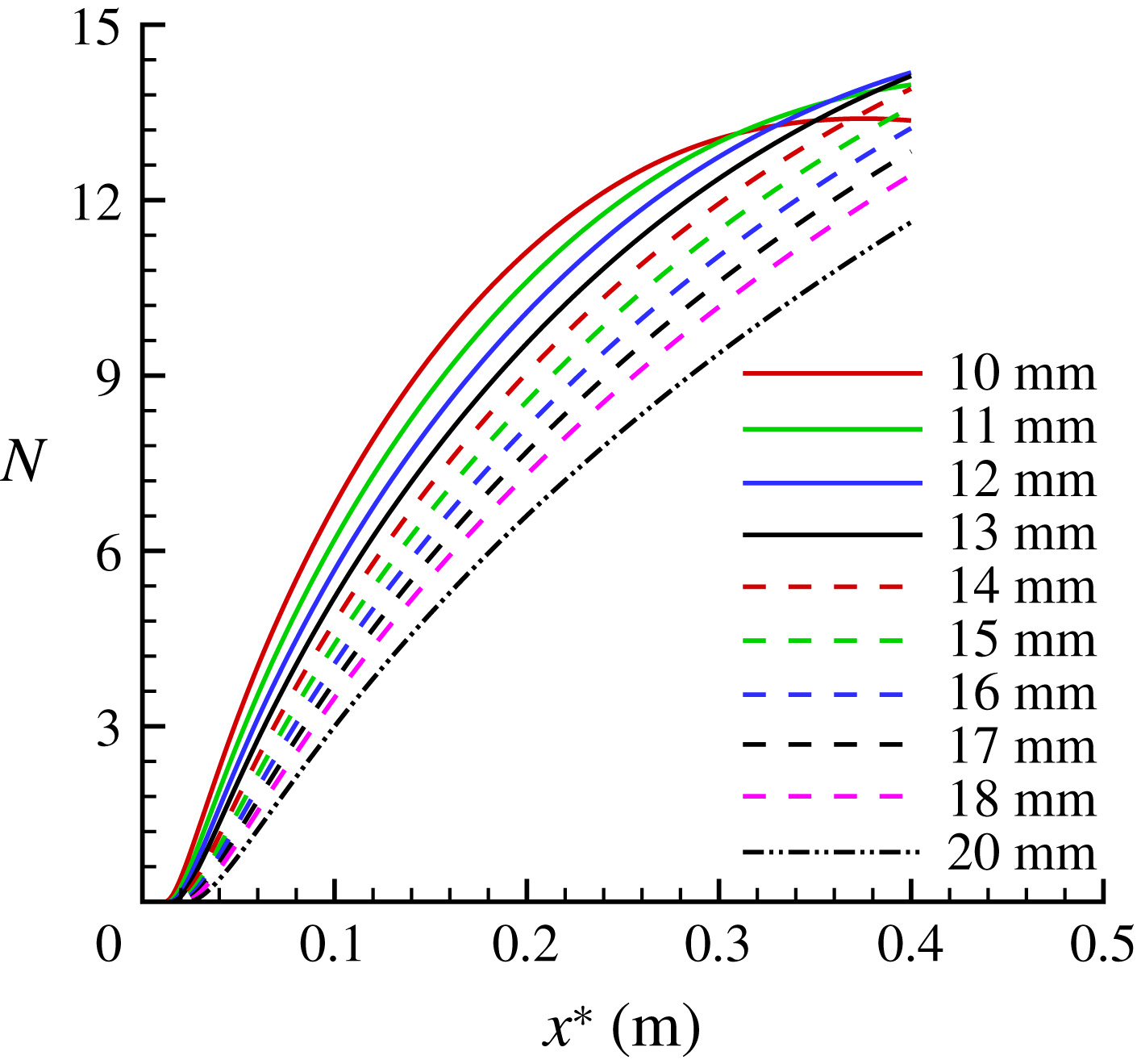
). The downstream evolutions of the stationary cross-flow modes in the hypersonic swept wing flow at Mach 6 are calculated with spatial LST. Figure 4 shows the
 $N$
factors of stationary cross-flow modes for several spanwise wavelengths,
 $$\begin{eqnarray}\displaystyle N=\int -\unicode[STIX]{x1D6FC}_{i}\,\text{d}\unicode[STIX]{x1D709}. & & \displaystyle\end{eqnarray}$$
It should be stressed that no unstable Tollmien–Schlichting waves and Mack modes are found in the flow studied herein due to the combination of the strong favourable pressure gradient in the chordwise direction and relatively low Mach number at the boundary edge as shown in figure 2(c).
The
 $N$
-factors of stationary cross-flow modes based on spatial LST for several spanwise wavelengths.

3.2 Nonlinear parabolized stability equations
On the other hand, in order to account for both non-parallel and nonlinear effects, the method of NPSE (Chang et al. Reference Chang, Malik, Erlebacher and Hussaini1991; Bertolotti, Herbert & Spalart Reference Bertolotti, Herbert and Spalart1992; Malik, Li & Chang Reference Malik, Li and Chang1994; Herbert Reference Herbert1997) is adopted to simulate the downstream evolution of the stationary cross-flow modes in the present study. In the NPSE framework, the cross-flow disturbance components, developing in the infinite spanwise swept wing flow, can be transformed in both the temporal and spanwise directions in the following manner,
 $$\begin{eqnarray}\displaystyle \unicode[STIX]{x1D753}(\unicode[STIX]{x1D709},\unicode[STIX]{x1D702},z,t)=\mathop{\sum }_{m=-\infty }^{\infty }\mathop{\sum }_{n=-\infty }^{\infty }\widehat{\unicode[STIX]{x1D711}}_{mn}(\unicode[STIX]{x1D709},\unicode[STIX]{x1D702})\exp \left[\text{i}\left(\int \unicode[STIX]{x1D6FC}_{mn}\,\text{d}\unicode[STIX]{x1D709}+n\unicode[STIX]{x1D6FD}z\text{i}m\unicode[STIX]{x1D714}t\right)\right], & & \displaystyle\end{eqnarray}$$
where
 $\widehat{\unicode[STIX]{x1D711}}_{mn}=(\widehat{\unicode[STIX]{x1D70C}}_{mn},\widehat{u}_{mn},\widehat{\unicode[STIX]{x1D710}}_{mn},\widehat{w}_{mn},\widehat{T}_{mn})$
represents the shape function and
 $\unicode[STIX]{x1D6FC}_{mn}$
denotes the streamwise wavenumber of the disturbance mode
 $(m,n)$
. On substituting (3.7) into (3.2) and neglecting the terms of order
 $1/Re^{2}$
(assuming that both the shape function
 $\widehat{\unicode[STIX]{x1D711}}_{mn}$
and
 $\unicode[STIX]{x1D6FC}_{mn}$
vary slowly with the marching direction
 $\unicode[STIX]{x1D709}$
), we can obtain the nonlinear parabolized stability equations for each mode
 $(m,n)$
:
 $$\begin{eqnarray}\displaystyle \overline{A}\frac{\unicode[STIX]{x2202}\widehat{\unicode[STIX]{x1D711}}_{mn}}{\unicode[STIX]{x2202}\unicode[STIX]{x1D709}}+\overline{B}\frac{\unicode[STIX]{x2202}\widehat{\unicode[STIX]{x1D711}}_{mn}}{\unicode[STIX]{x2202}\unicode[STIX]{x1D702}}+\overline{D}\widehat{\unicode[STIX]{x1D711}}_{mn}=H_{\unicode[STIX]{x1D702}\unicode[STIX]{x1D702}}\frac{\unicode[STIX]{x2202}^{2}\widehat{\unicode[STIX]{x1D711}}_{mn}}{\unicode[STIX]{x2202}\unicode[STIX]{x1D702}^{2}}+F_{mn}/\exp \left(\text{i}\int \unicode[STIX]{x1D6FC}_{mn}\,\text{d}\unicode[STIX]{x1D709}\right). & & \displaystyle\end{eqnarray}$$
The vector
 $F_{mn}$
represents the Fourier component of the nonlinear terms which can be obtained with fast Fourier transform in the physical space. The governing equations are discretized by a second-order implicit finite difference along the
 $\unicode[STIX]{x1D709}$
direction and by a fourth-order central difference in the wall-normal direction. The details of the NPSE method and its verification can be found in Xu et al. (Reference Xu, Xiao and Fu2011) or Ren & Fu (Reference Ren and Fu2015).
3.3 Secondary linear stability theory (SLST)
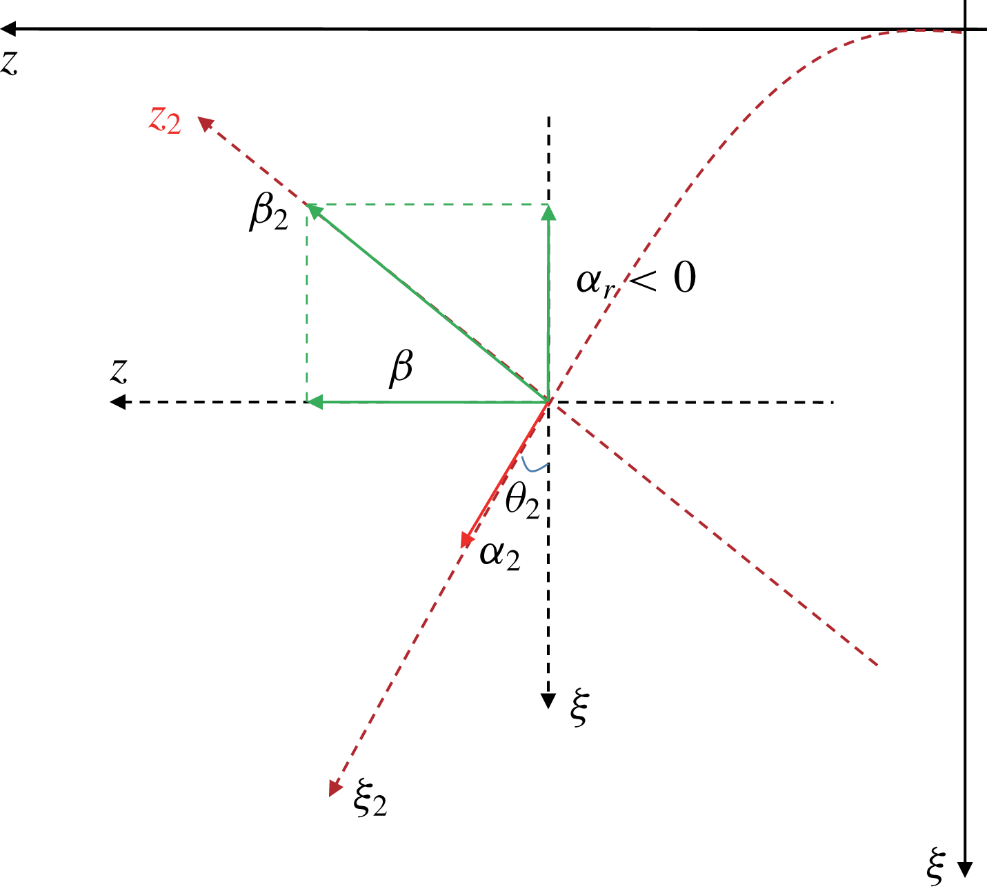
Definition of the vortex-oriented coordinate system.

The three-dimensional boundary layer flow will be distorted by the stationary cross-flow vortex with large amplitudes; the highly inflectional velocity profiles of the new base flow are the cause of this secondary cross-flow instability. The new base flow
 $Q_{2}$
, is formed by a superposition of the laminar boundary layer flow and solutions of the primary disturbances from NPSE computation,
 $$\begin{eqnarray}\displaystyle \left.\begin{array}{@{}c@{}}Q_{2}=(\unicode[STIX]{x1D70C}_{2},U_{2},V_{2},W_{2},T_{2})\\ Q_{2}=Q+\unicode[STIX]{x1D753}_{NPSE}.\end{array}\right\} & & \displaystyle\end{eqnarray}$$
Assuming that the new base flow
 $Q_{2}$
varies slowly along the vortex axis (
 $\unicode[STIX]{x1D709}_{2}$
-direction), then
 $$\begin{eqnarray}\displaystyle Q_{2}(\unicode[STIX]{x1D702}_{2},z_{2})=Q(\unicode[STIX]{x1D702}_{2},z_{2})+\mathop{\sum }_{n=-\infty }^{\infty }\widehat{\unicode[STIX]{x1D711}}_{n}(\unicode[STIX]{x1D702}_{2})(\unicode[STIX]{x1D702}_{2},z_{2})\exp (\text{i}n\unicode[STIX]{x1D6FD}_{2}z_{2}), & & \displaystyle\end{eqnarray}$$
where
 $\unicode[STIX]{x1D702}_{2}$
and
 $z_{2}$
represent the wall-normal and the wave vector direction, respectively;
 $\unicode[STIX]{x1D6FD}_{2}$
denoting the fundamental spanwise wavenumber of the stationary cross-flow vortex along the wave vector
 $z_{2}$
direction as shown in figure 5, is given as
 $$\begin{eqnarray}\displaystyle \unicode[STIX]{x1D6FD}_{2}=\sqrt{\unicode[STIX]{x1D6FC}_{r}^{2}+\unicode[STIX]{x1D6FD}^{2}}, & & \displaystyle\end{eqnarray}$$
wherein,
 $\unicode[STIX]{x1D6FC}_{r}$
and
 $\unicode[STIX]{x1D6FD}$
are the chordwise and spanwise wavenumbers corresponding to the fundamental stationary cross-flow mode in the body fitted orthogonal coordinate system. In figure 5,
 $\unicode[STIX]{x1D703}_{2}$
is the angle of the stationary cross-flow vortex direction in the vortex-oriented coordinates
 $$\begin{eqnarray}\displaystyle \tan (\unicode[STIX]{x1D703}_{2})=\frac{|\unicode[STIX]{x1D6FC}_{r}|}{\unicode[STIX]{x1D6FD}}. & & \displaystyle\end{eqnarray}$$
In the present work, the secondary instabilities of stationary cross-flow vortices are investigated using the Floquet theory since the new basic flow
 $Q_{2}$
is periodic along the wave vector
 $z_{2}$
direction. The secondary instability modes are given in the Fourier expansion form adopted by Malik et al. (Reference Malik, Li, Choudhari and Chang1999), Koch et al. (Reference Koch, Bertolotti, Stolte and Hein2000),
 $$\begin{eqnarray}\displaystyle \left.\begin{array}{@{}c@{}}\displaystyle \unicode[STIX]{x1D753}_{2}(\unicode[STIX]{x1D709}_{2},\unicode[STIX]{x1D702},z_{2},t)=\text{e}^{\text{i}(\unicode[STIX]{x1D6FC}_{2}\unicode[STIX]{x1D709}_{2}+\unicode[STIX]{x1D6FE}\unicode[STIX]{x1D6FD}_{2}z_{2})}\text{e}^{\unicode[STIX]{x1D714}_{2}t}\mathop{\sum }_{m_{2}=-M_{2}}^{+M_{2}}\widehat{\unicode[STIX]{x1D711}}_{2,n_{2}}(\unicode[STIX]{x1D702},z_{2})\text{e}^{\text{i}m_{2}\unicode[STIX]{x1D6FD}_{2}z_{2}}+\text{c.c.}\\ \unicode[STIX]{x1D753}_{2}=(\unicode[STIX]{x1D70C}_{2}^{\prime },u_{2}^{\prime },\unicode[STIX]{x1D710}_{2}^{\prime },w_{2}^{\prime },T_{2}^{\prime }).\end{array}\right\} & & \displaystyle\end{eqnarray}$$
Utilizing the temporal framework in the instability analysis, the real part of
 $\unicode[STIX]{x1D714}_{2}$
represents the growth rate, and its imaginary part the frequency, and
 $\unicode[STIX]{x1D6FC}_{2}$
are the streamwise wavenumbers of secondary instability modes in the vortex-oriented coordinates. In fact, the Floquet analysis is the classic LST method for two-dimensional flows. Substituting (3.10) and (3.13) as the basic flow and disturbances into (3.2), dropping the nonlinear term and
 $\unicode[STIX]{x2202}Q_{2}/\unicode[STIX]{x2202}\unicode[STIX]{x1D709}_{2}$
, the SLST equations reduce to a generalized eigenvalue problem. For the numerical computation of the eigenvalue problem, the SLST equations are discretized in the wall-normal direction via fourth-order central difference. More details of the validation of the present Floquet analysis can be found in Xu et al. (Reference Xu, Xiao and Fu2011, Reference Xu, Liu, Chen and Fu2018a
) or Ren & Fu (Reference Ren and Fu2015). Xu et al. (Reference Xu, Liu, Chen and Fu2018a
) had shown that the secondary cross-flow instability results in compressible three-dimensional boundary layers were almost independent of the Floquet parameter
 $\unicode[STIX]{x1D6FE}$
. Thus,
 $\unicode[STIX]{x1D6FE}=0$
is prescribed in the instability calculation.
4 Results
4.1 Nonlinear saturation of stationary cross-flow modes at the hypersonic swept wing
For the stationary cross-flow vortex of concern here, we choose the stationary cross-flow mode with spanwise wavelength 10 mm to be the fundamental mode, because this mode first reaches an N-factor of 5 (as shown in figure 4), which is believed to be the critical transition location (for instance, King (Reference King1992), Malik & Balakumar (Reference Malik and Balakumar1992), Owens et al. (Reference Owens, Beeler, Balakumar and McGuire2014)). Then, the downstream evolution of the stationary cross-flow modes can be resolved by NPSE. Computations start at
 $x^{\ast }=0.04~\text{m}$
(near the leading edge), and the initial amplitudes of the fundamental stationary cross-flow mode are set to
 $|\widehat{u}_{01}|=5\times 10^{-5}$
and
 $10^{-4}$
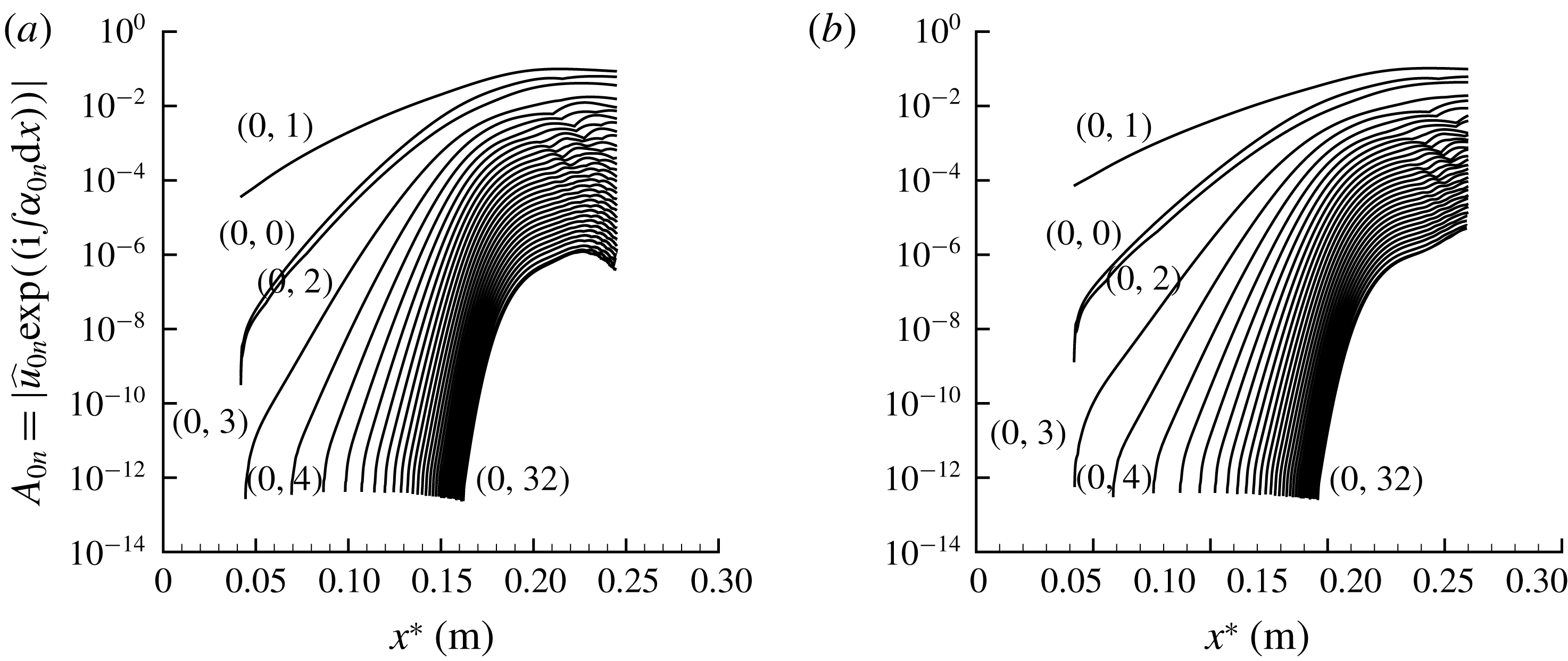
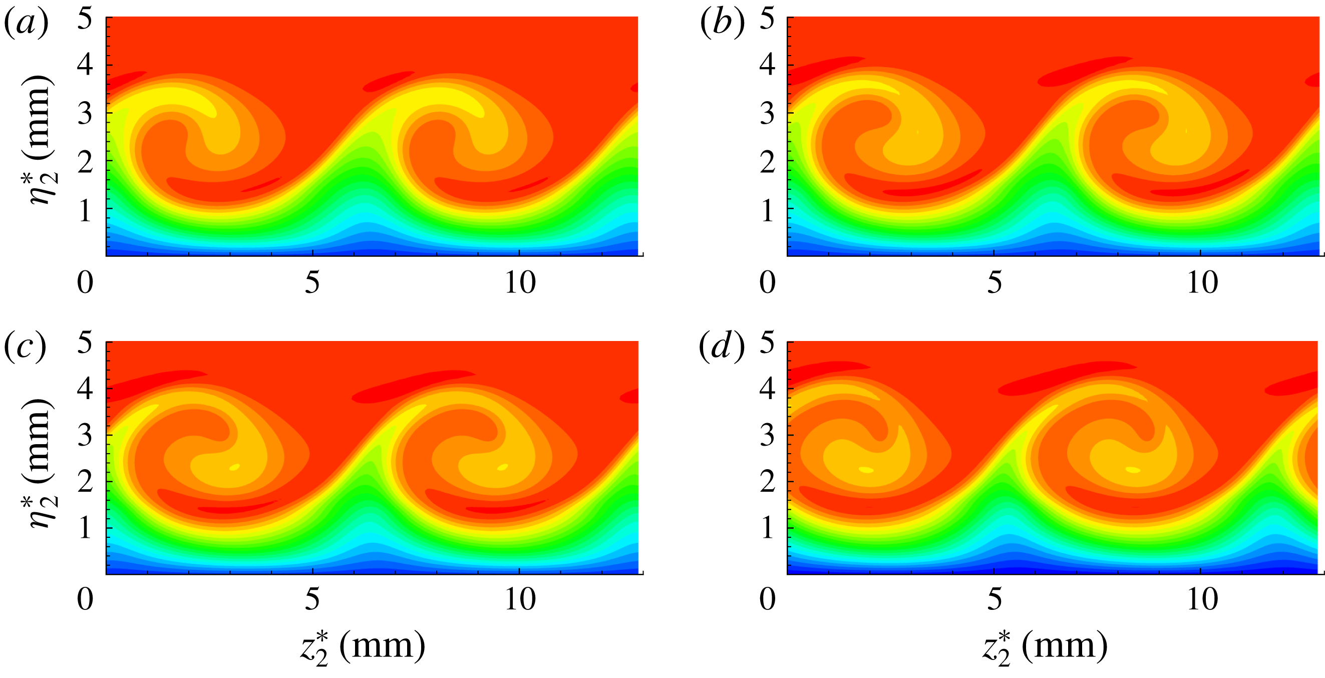
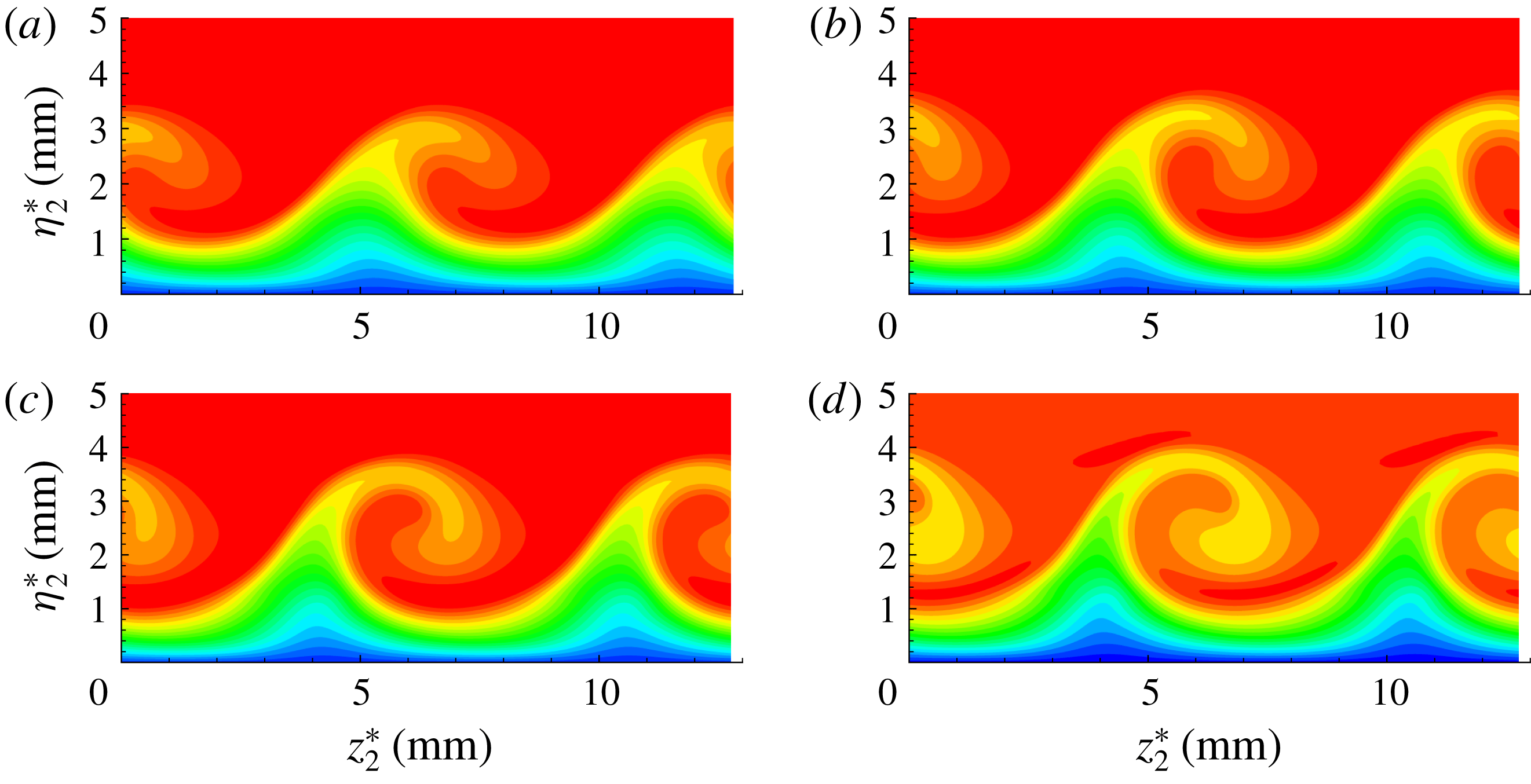
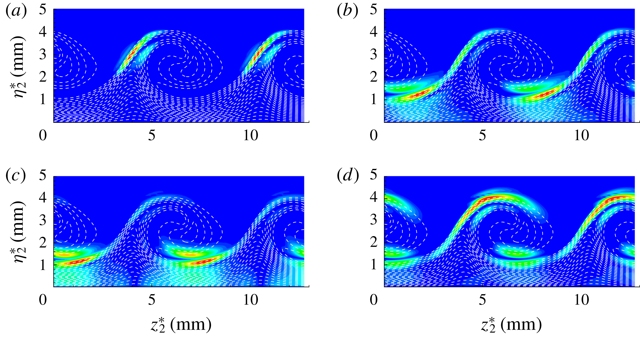
, respectively. For the NPSE simulations, the chordwise grid consists of 48 uniformly distributed points within a fundamental wavelength; 401 points are distributed along the wall-normal direction and 32 Fourier modes are used in the spanwise direction. Figures 6(a) and 6(b), respectively show the evolution of the velocity disturbance amplitude of stationary cross-flow modes for two initial amplitudes. Both of the stationary cross-flow modes experienced a linear growth and then a saturated period due to the nonlinear effect. Figure 7(a–d), respectively, shows the resulting boundary layers distorted by stationary cross-flow vortices in the vortex-oriented system at
 $x^{\ast }=0.208~\text{m}$
, 0.22 m, 0.23 m, 0.24 m for the case with
 $A_{01}=5\times 10^{-5}$
, whereas figure 8(a–d) gives the same results for the case with
 $A_{01}=1\times 10^{-4}$
at
 $x^{\ast }=0.178~\text{m}$
, 0.187 m, 0.198 m, 0.208 m, respectively. It can be seen that the initial amplitude of the fundamental mode has little influence on the spatial distributions of stationary cross-flow vortex in the saturated region.
Evolution of stationary cross-flow modes with initial amplitude: (a)
 $A_{01}=5\times 10^{-5}$
; (b)
 $A_{01}=10^{-4}$
.

The spatial distributions of vortex velocity
 $U_{2}$
in the cross-section plane with
 $A_{01}=5\times 10^{-5}$
: (a) at
 $x^{\ast }=0.208~\text{m}$
, (b) at
 $x^{\ast }=0.22~\text{m}$
, (c) at
 $x^{\ast }=0.23~\text{m}$
, (d) at
 $x^{\ast }=0.24~\text{m}$
.

The spatial distributions of vortex velocity
 $U_{2}$
in the cross-section plane with
 $A_{01}=10^{-4}$
: (a) at
 $x^{\ast }=0.178~\text{m}$
, (b) at
 $x^{\ast }=0.187~\text{m}$
, (c) at
 $x^{\ast }=0.198~\text{m}$
, (d) at
 $x^{\ast }=0.208~\text{m}$
.

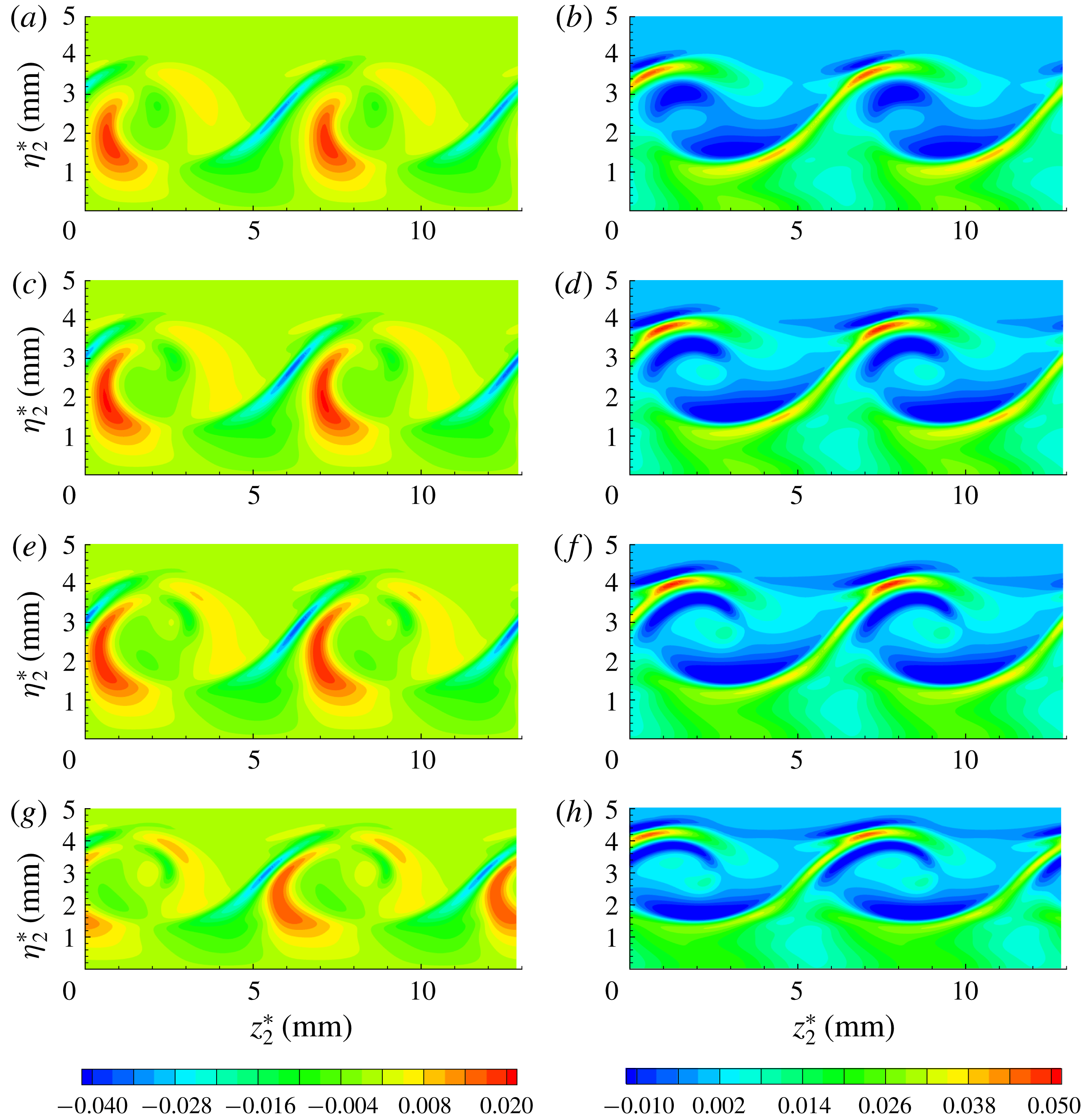
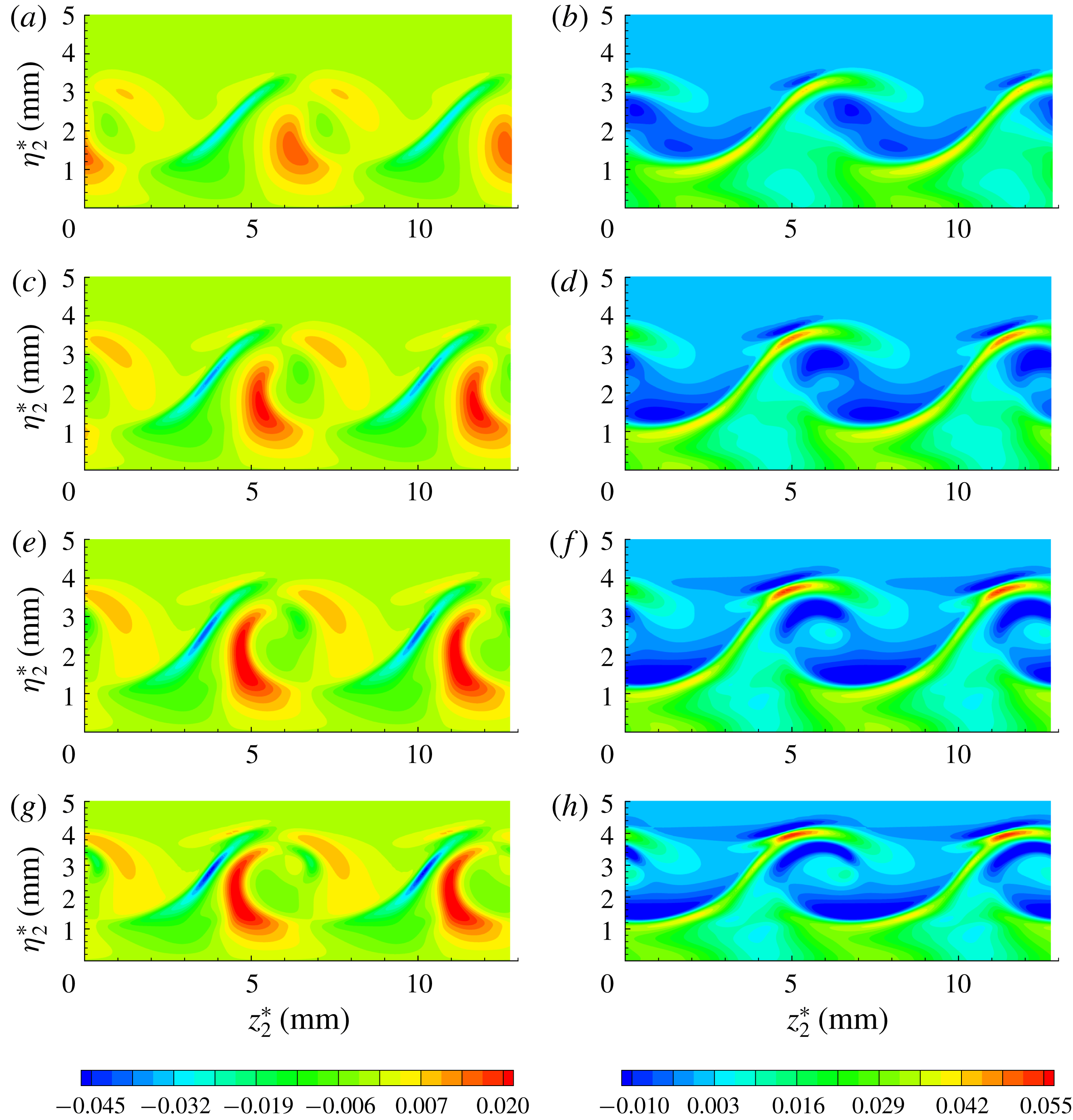
It is well known that the laminar–turbulent transition of the stationary cross-flow vortex inside swept wing flows can be directly triggered by secondary cross-flow instability modes. These modes can extract the energy through the spanwise shear or wall-normal shear of the modified basic state as shown by Malik et al. (Reference Malik, Li, Choudhari and Chang1999). Thereby, the generalized gradients of vortex velocity
 $U_{2}$
are depicted in figures 9 and 10 for these two cases, respectively. According to the locations of the minimum spanwise gradients, as shown in figures 9(a,c,e,g) and 10(a,c,e,g), it is therefore likely that the ‘z’ mode will concentrate on the shoulder of the stationary cross-flow vortex, which is the same as in incompressible swept wing flows. However, as illustrated in figures 9(b,d,f,h) and 10(b,d,f,h), in addition to the maximum wall-normal gradients on the crest of the stationary cross-flow vortex as in incompressible swept wing flows (Malik et al.
Reference Malik, Li, Choudhari and Chang1999; Koch et al.
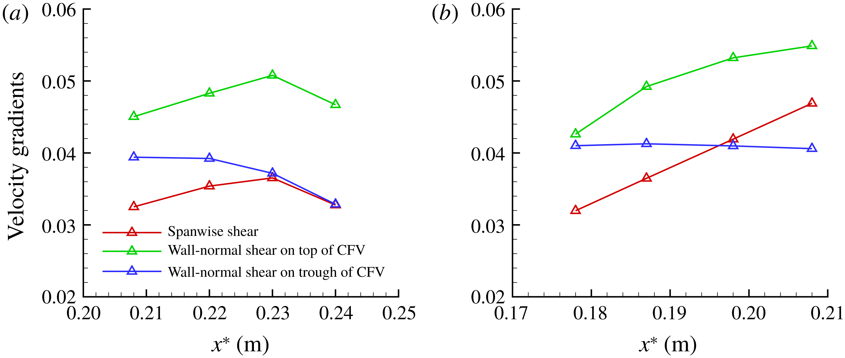
Reference Koch, Bertolotti, Stolte and Hein2000; Wassermann & Kloker Reference Wassermann and Kloker2002; White & Saric Reference White and Saric2005), there is another maximum wall-normal gradient, but close to the trough of the stationary cross-flow vortex. Furthermore, the presence of maximum wall-normal gradients close to the trough of the stationary cross-flow vortex is independent of the initial amplitude of the fundamental cross-flow mode and chordwise position. Figure 11 shows the variations of the extremum magnitude of the spanwise shear and wall-normal shear with chordwise position for these two cases. We may infer that the ‘y’ mode can also be excited on the trough of stationary cross-flow vortex. In fact, the maximum wall-normal gradient on the trough of the stationary cross-flow vortex in a hypersonic pitched cone was also noticed by Moyes et al. (Reference Moyes, Paredes, Kocian and Reed2017), who suggested that the ‘y’ mode should have been excited on the trough of the stationary cross-flow vortex. However, only the ‘y’ mode on top of the stationary cross-flow vortex was found by Moyes et al. (Reference Moyes, Paredes, Kocian and Reed2017) through bi-global instability analysis.
Contours of the generalized gradients of vortex velocity
 $U_{2}$
for the case with
 $A_{01}=5\times 10^{-5}$
. (a)
 $\unicode[STIX]{x1D70C}_{2}\unicode[STIX]{x2202}U_{2}/\unicode[STIX]{x2202}z_{2}$
and (b)
 $\unicode[STIX]{x1D70C}_{2}\unicode[STIX]{x2202}U_{2}/\unicode[STIX]{x2202}\unicode[STIX]{x1D702}_{2}$
at
 $x^{\ast }=0.208~\text{m}$
; (c)
 $\unicode[STIX]{x1D70C}_{2}\unicode[STIX]{x2202}U_{2}/\unicode[STIX]{x2202}z_{2}$
and (d)
 $\unicode[STIX]{x1D70C}_{2}\unicode[STIX]{x2202}U_{2}/\unicode[STIX]{x2202}\unicode[STIX]{x1D702}_{2}$
at
 $x^{\ast }=0.22~\text{m}$
; (e)
 $\unicode[STIX]{x1D70C}_{2}\unicode[STIX]{x2202}U_{2}/\unicode[STIX]{x2202}z_{2}$
and (f)
 $\unicode[STIX]{x1D70C}_{2}\unicode[STIX]{x2202}U_{2}/\unicode[STIX]{x2202}\unicode[STIX]{x1D702}_{2}$
at
 $x^{\ast }=0.23~\text{m}$
; (g)
 $\unicode[STIX]{x1D70C}_{2}\unicode[STIX]{x2202}U_{2}/\unicode[STIX]{x2202}z_{2}$
and (h)
 $\unicode[STIX]{x1D70C}_{2}\unicode[STIX]{x2202}U_{2}/\unicode[STIX]{x2202}\unicode[STIX]{x1D702}_{2}$
at
 $x^{\ast }=0.24~\text{m}$
.

Contours of the generalized gradients of vortex velocity
 $U_{2}$
for the case with
 $A_{01}=10^{-4}$
. (a)
 $\unicode[STIX]{x1D70C}_{2}\unicode[STIX]{x2202}U_{2}/\unicode[STIX]{x2202}z_{2}$
and (b)
 $\unicode[STIX]{x1D70C}_{2}\unicode[STIX]{x2202}U_{2}/\unicode[STIX]{x2202}\unicode[STIX]{x1D702}_{2}$
at
 $x^{\ast }=0.178~\text{m}$
; (c)
 $\unicode[STIX]{x1D70C}_{2}\unicode[STIX]{x2202}U_{2}/\unicode[STIX]{x2202}z_{2}$
and (d)
 $\unicode[STIX]{x1D70C}_{2}\unicode[STIX]{x2202}U_{2}/\unicode[STIX]{x2202}\unicode[STIX]{x1D702}_{2}$
at
 $x^{\ast }=0.187~\text{m}$
; (e)
 $\unicode[STIX]{x1D70C}_{2}\unicode[STIX]{x2202}U_{2}/\unicode[STIX]{x2202}z_{2}$
and (f)
 $\unicode[STIX]{x1D70C}_{2}\unicode[STIX]{x2202}U_{2}/\unicode[STIX]{x2202}\unicode[STIX]{x1D702}_{2}$
at
 $x^{\ast }=0.198~\text{m}$
; (g)
 $\unicode[STIX]{x1D70C}_{2}\unicode[STIX]{x2202}U_{2}/\unicode[STIX]{x2202}z_{2}$
and (h)
 $\unicode[STIX]{x1D70C}_{2}\unicode[STIX]{x2202}U_{2}/\unicode[STIX]{x2202}\unicode[STIX]{x1D702}_{2}$
at
 $x^{\ast }=0.208~\text{m}$
.

(a) Variations of the extremum magnitude of the spanwise and wall-normal shear along the chordwise position for the case with
 $A_{01}=5\times 10^{-5}$
; (b) variations of the spanwise and wall-normal shear with chordwise position for the case with
 $A_{01}=10^{-4}$
. CFV represents cross-flow vortex; note that the generalized gradients are used.

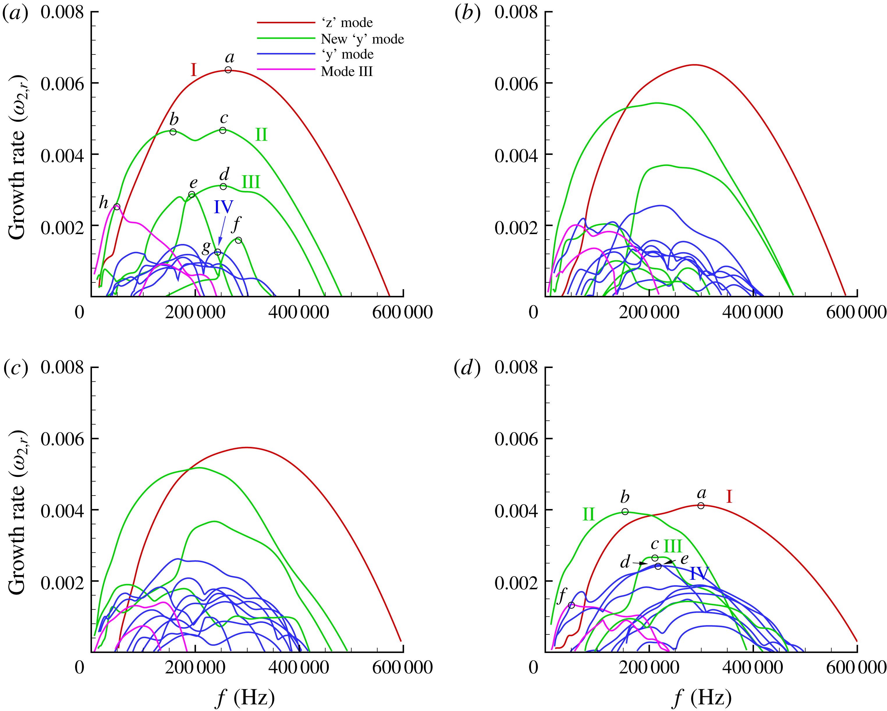
The growth rates of cross-flow secondary instability modes as a function of frequency: (a) at
 $x^{\ast }=0.208~\text{m}$
, (b) at
 $x^{\ast }=0.22~\text{m}$
, (c) at
 $x^{\ast }=0.23~\text{m}$
, (d) at
 $x^{\ast }=0.24~\text{m}$
.

4.2 Secondary instabilities of stationary cross-flow vortices at the hypersonic swept wing
The stationary cross-flow vortices obtained in the previous section are employed to implement the secondary instability analysis through the Floquet theory. For the case with
 $A_{01}=5\times 10^{-5}$
, the calculations of the secondary instability theory are carried out for the stationary cross-flow vortex at
 $x^{\ast }=0.208~\text{m}$
, 0.22 m, 0.23 m and 0.24 m. Table 2 depicts a grid convergence study on the growth rates of the most unstable secondary instability modes at
 $x^{\ast }=0.208~\text{m}$
with
 $\unicode[STIX]{x1D6FC}_{2}=0.20$
. It is demonstrated that a number of
 $Ny_{2}=201$
points in the wall-normal direction and
 $M_{2}=20$
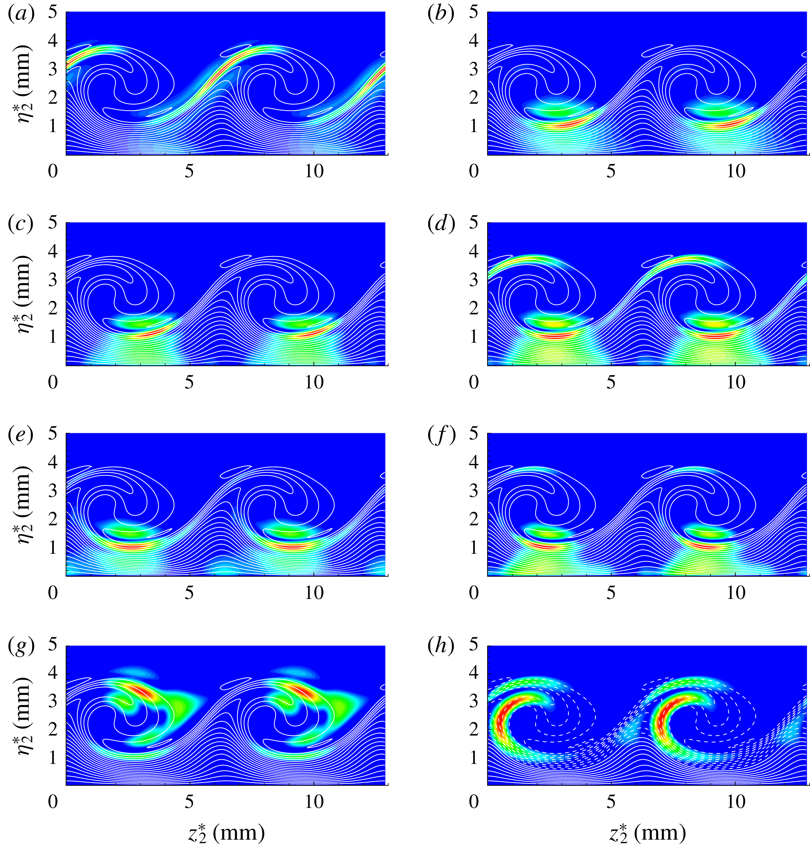
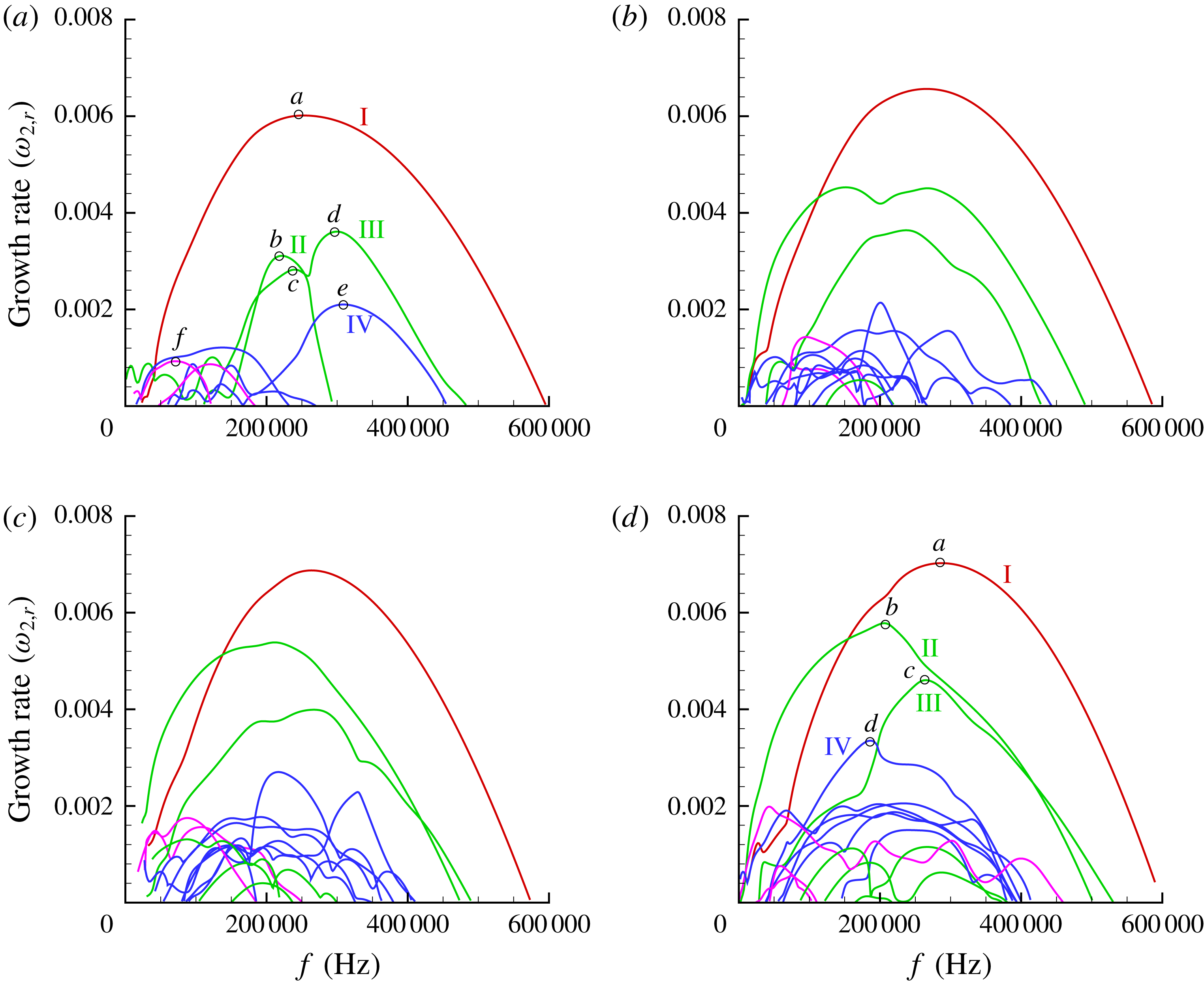
spanwise Fourier modes along the spanwise direction are sufficient to resolve all unstable modes based on grid convergence analysis. Figure 12(a–d) shows the growth rates of secondary instability modes as a function of frequency at these four chordwise positions, respectively. In the present work, four different categories of secondary instability modes denoted by the red, green, blue and magenta lines are captured through SLST. The contours of
 $|u_{2}^{\prime }|$
of the secondary instability modes of the stationary cross-flow vortex at
 $x^{\ast }=0.208~\text{m}$
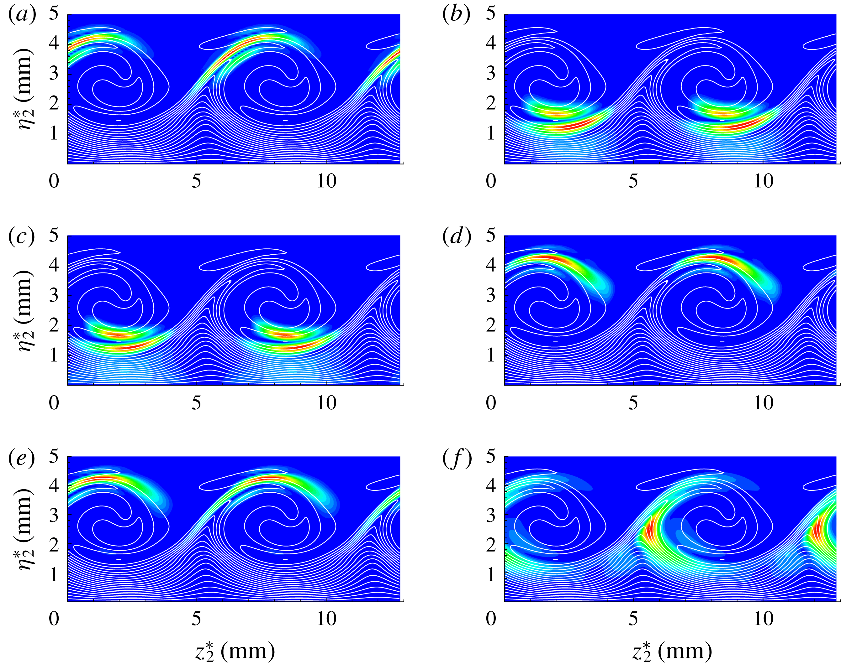
are presented in figure 13. They are obtained at selected growth rate peaks labelled by the letters (a–h) in figure 12(a). Figure 14 shows the same results at
 $x^{\ast }=0.24~\text{m}$
, but with growth rate peaks labelled by the letters (a–f) in figure 12(d). Figures 13(a) and 14(a) demonstrate that the highest velocity disturbances of the secondary instability modes denoted by red lines in figure 12 are concentrated on the shoulder of the stationary cross-flow vortex, indicating that these secondary instability modes belong to the class of ‘z’ mode. As in low-speed swept wing flows (Koch et al.
Reference Koch, Bertolotti, Stolte and Hein2000; Wassermann & Kloker Reference Wassermann and Kloker2002; White & Saric Reference White and Saric2005), the ‘z’ mode is the most unstable mode. According to figures 13(g) and 14(d,e), it is easy to confirm that the secondary instability modes denoted by blue lines in figure 12 are ‘y’ modes, since their velocity disturbances concentrate at the top of the stationary cross-flow vortex. Moreover, figures 13(h) and 14(f) display the velocity mode shapes of the secondary instability modes represented by magenta lines in figure 12. Obviously, velocity fluctuations are mainly concentrated around the maximum spanwise gradient of the modified basic flow as shown in figure 9(a,c,e,g). Therefore, it can be inferred that the magenta lines in figure 12 stand for the low-frequency mode (Wassermann & Kloker Reference Wassermann and Kloker2002; White & Saric Reference White and Saric2005).
The
 $|u_{2}^{\prime }|$
-eigenfunction of the secondary instability modes at peak growth rate for the case with
 $A_{01}=10^{-5}$
, at
 $x^{\ast }=0.208~\text{m}$
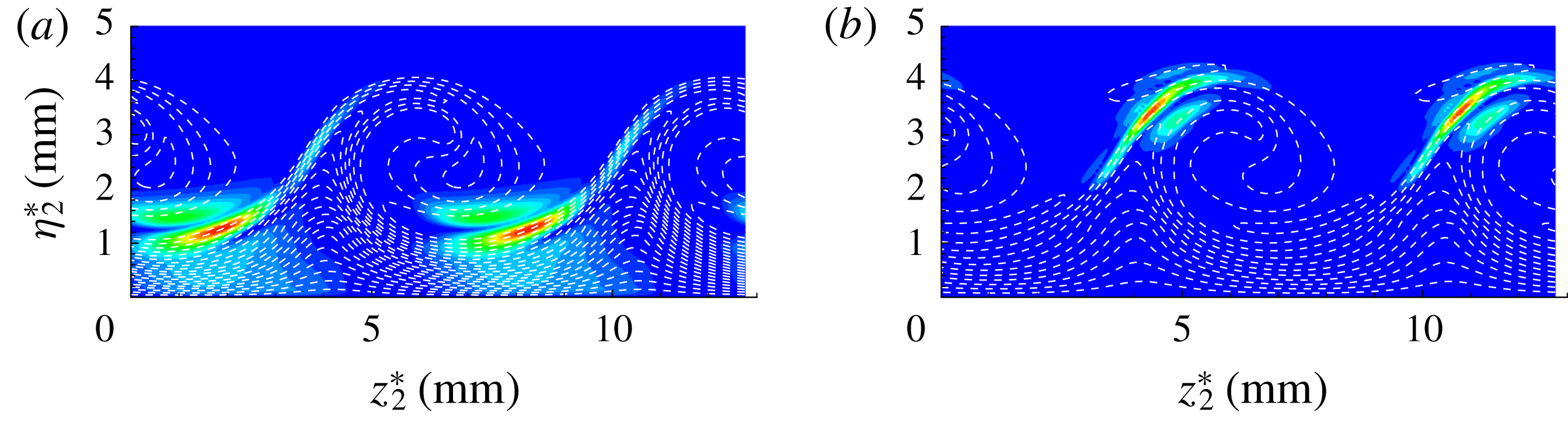
. White dash lines represent the stationary cross-flow vortex.

Variation of growth rates of the highest unstable modes (eig1, most unstable mode; eig2, second most unstable mode) with grid.

The
 $|u_{2}^{\prime }|$
-eigenfunction of the secondary instability modes at peak growth rate for the case with
 $A_{01}=10^{-5}$
, at
 $x^{\ast }=0.24~\text{m}$
. White dash lines represent the stationary cross-flow vortex.

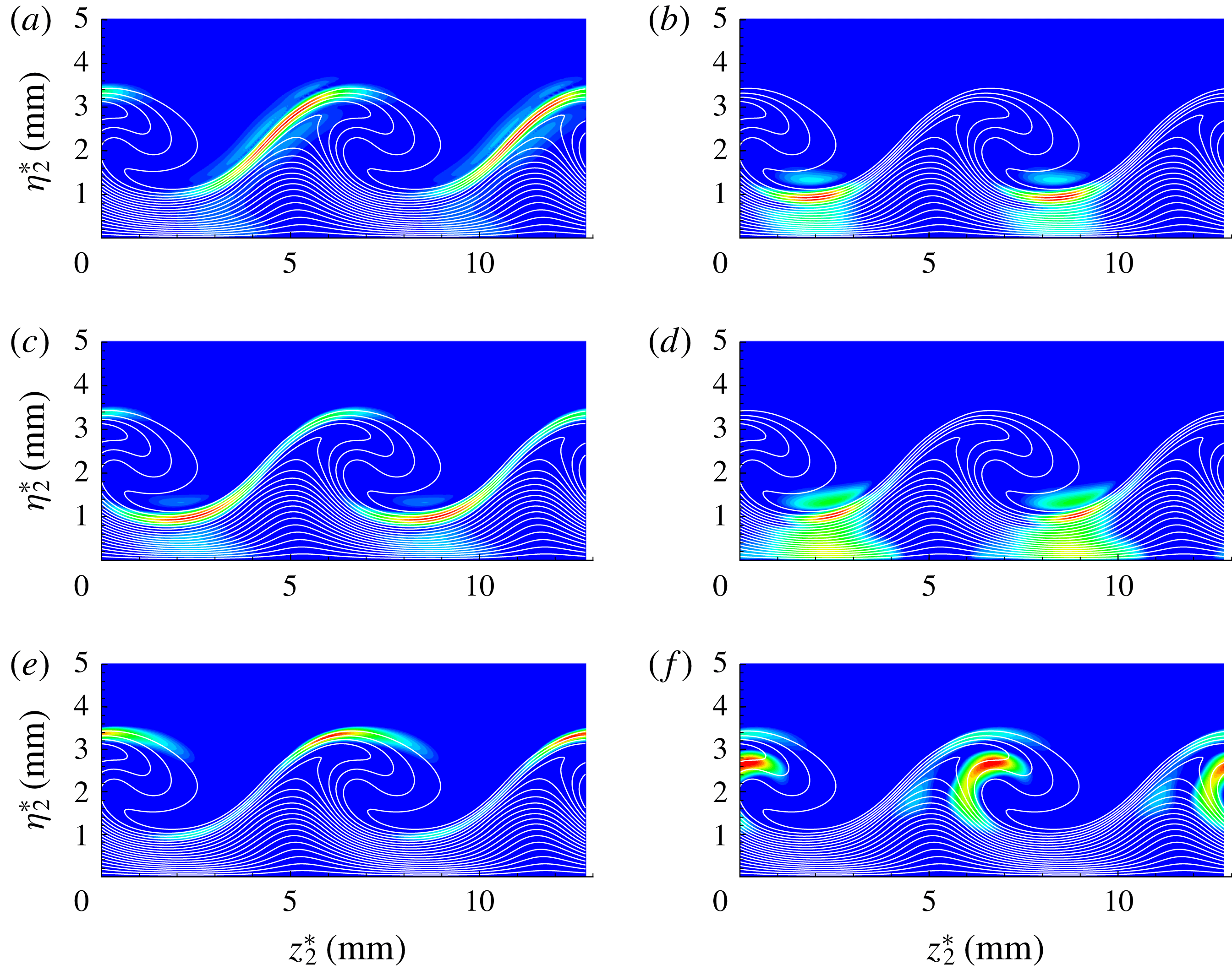
An important finding of the present study is a new type secondary instability mode denoted by green lines in figure 12. The normalized velocity distributions of this new mode are plotted in figures 13(b–f) and 14(b,c) at two different chordwise locations. It can be found that this new secondary instability mode is strongly connected to the maximum wall-normal gradient, but is located near the trough of the stationary cross-flow vortex instead of at the top, indicating that it belongs to the class of ‘y’ mode. This new ‘y’ mode is absent in incompressible swept wing flows. Thus, to distinguish them, the ‘y’ modes residing at the trough and the top of a stationary cross-flow vortex are here called new and traditional ‘y’ modes, respectively. It is noted in figure 11 that the magnitude of the wall-normal shear at the trough of the stationary cross-flow vortex is smaller than that at the crest, but the growth rates of the new ‘y’ mode and the ‘z’ mode are comparable, and are much larger than that of the traditional ‘y’ mode according to figure 12.
The growth rates of cross-flow secondary instability modes as a function of frequency; (a) at
 $x^{\ast }=0.178~\text{m}$
, (b) at
 $x^{\ast }=0.187~\text{m}$
, (c) at
 $x^{\ast }=0.198~\text{m}$
, (d) at
 $x^{\ast }=0.208~\text{m}$
.

For the case with
 $A_{01}=10^{-4}$
, the calculations of the secondary instability theory are carried out in the same way as for the stationary cross-flow vortex at
 $x^{\ast }=0.178~\text{m}$
, 0.187 m, 0.198 m and 0.208 m. Figure 15(a–d) shows the growth rates of the secondary instability modes as a function of frequency at these four chordwise positions, respectively. The ‘z’ mode, new ‘y’ mode, traditional ‘y’ mode and low-frequency mode are also denoted by red, green, blue and magenta lines, respectively. Similar to the lower initial amplitude case, the ‘z’ mode is still the most unstable mode. Moreover, the new ‘y’ mode, which has a comparable growth rate to the ‘z’ mode, is much more unstable than the traditional ‘y’ mode. The contours of
 $|u_{2}^{\prime }|$
of these secondary instability modes of the stationary cross-flow vortex at
 $x^{\ast }=0.178~\text{m}$
with growth rate peaks denoted by letters (a–f) in figure 15(a) are also presented in figure 16(a–f), respectively. More evidence for the existence of the new ‘y’ mode can be seen in figure 16(b–d). Figure 16(e) shows the spatial distribution of the velocity mode shape of the ‘y’ mode at the top of a stationary cross-flow, and unstable low-frequency modes can also be found according to the mode shape as presented in figure 16(f). In fact, a secondary instability mode (‘mode III’) which is located in the region of locally large wall-normal gradients near the trough was shown in figure 16 by Koch et al. (Reference Koch, Bertolotti, Stolte and Hein2000). However, note that this mode in Koch et al. (Reference Koch, Bertolotti, Stolte and Hein2000) is a low-frequency mode, whereas the new ‘y’ mode in the present work has a frequency comparable to the ‘y’ and ‘z’ modes as shown in figures 12 and 15.
Figure 17(a–d) shows the mode shapes of velocity disturbances of the secondary instability modes at
 $x^{\ast }=0.208~\text{m}$
, labelled as (a–d) in the figure 15(d), respectively. The ‘z’ mode denoted by the red line in figure 15(d) is also the most unstable, concentrating on the shoulder of the stationary cross-flow vortex as shown in figure 17(a). The new ‘y’ modes denoted by the green lines in figure 15(d), are also excited according to figure 17(b,c). As presented in figure 17(b), it may be interesting to find that the velocity fluctuations of the new ‘y’ mode distributed at the shoulder of the stationary cross-flow cannot be neglected, indicating that this mode is also driven by the spanwise shear. According to figure 17(d), it can be seen that the secondary instability mode denoted by blue line in figure 15(d) may be the mixed ‘y’/‘z’ mode, since its velocity fluctuations are concentrated on both the top and shoulder of the stationary cross-flow vortex. In fact, the mixed ‘y’/‘z’ modes located at both the top and shoulder of the stationary cross-flow vortex were also observed by Choudhari et al. (Reference Choudhari, Li, Duan, Chang, Carpenter, Streett and Malik2013).
The
 $|u_{2}^{\prime }|$
-eigenfunction of the secondary instability modes at peak growth rate for the case with
 $A_{01}=10^{-4}$
, at
 $x^{\ast }=0.178~\text{m}$
. White dash lines represent the stationary cross-flow vortex.

The
 $|u_{2}^{\prime }|$
-eigenfunction of the secondary instability modes at peak growth rate for the case with
 $A_{01}=10^{-4}$
, at
 $x^{\ast }=0.208~\text{m}$
. White dash lines represent the stationary cross-flow vortex.

4.3 Kinetic energy budget
To provide further insight into the instability dynamics of the secondary instability modes in the hypersonic three-dimensional boundary layer flows, a balance analysis of the kinetic energy budget for cross-flow secondary instability modes is carried out. The contributions of compressibility to the growth of the secondary instability modes are also examined. In fact, the balance analysis for cross-flow secondary instability modes in incompressible swept wing flow had been given by Malik et al. (Reference Malik, Li, Choudhari and Chang1999). According to the momentum equations of the compressible Navier–Stokes equations, the equation of disturbance kinetic energy can be written as
 $$\begin{eqnarray}\displaystyle \unicode[STIX]{x1D70C}\frac{\text{D}(u_{i}^{\prime }u_{i}^{\prime }/2)}{\text{D}t}=-\unicode[STIX]{x1D70C}u_{i}^{\prime }u_{j}^{\prime }\frac{\unicode[STIX]{x2202}U_{i}}{\unicode[STIX]{x2202}x_{j}}-\unicode[STIX]{x1D70C}^{\prime }u_{i}^{\prime }U_{j}\frac{\unicode[STIX]{x2202}U_{i}}{\unicode[STIX]{x2202}x_{j}}-\frac{\unicode[STIX]{x2202}p^{\prime }u_{i}^{\prime }}{\unicode[STIX]{x2202}x_{i}}+p^{\prime }\frac{\unicode[STIX]{x2202}u_{i}^{\prime }}{\unicode[STIX]{x2202}x_{i}}+\frac{1}{Re}u_{i}^{\prime }\frac{\unicode[STIX]{x2202}\unicode[STIX]{x1D70F}_{ij}^{\prime }}{\unicode[STIX]{x2202}x_{j}}. & & \displaystyle\end{eqnarray}$$
Integrating the kinetic energy equation over the domain for the normal modes of (4.1), we can get
 $$\begin{eqnarray}\displaystyle \left.\begin{array}{@{}c@{}}2\unicode[STIX]{x1D714}_{2,r}E_{k}=\text{d}E_{k}/\text{d}t=P_{k}+\unicode[STIX]{x1D6EF}+D_{iff}+\unicode[STIX]{x1D6F1}+\unicode[STIX]{x1D700}\\ \unicode[STIX]{x1D714}_{2,r}=0.5(P+\unicode[STIX]{x1D6EF}+D_{iff}+\unicode[STIX]{x1D6F1}+\unicode[STIX]{x1D700})/E_{k},\end{array}\right\} & & \displaystyle\end{eqnarray}$$
where
 $$\begin{eqnarray}\displaystyle E_{k}=\int _{0}^{2\unicode[STIX]{x03C0}/\unicode[STIX]{x1D6FD}_{2}}\int _{0}^{\infty }\int _{0}^{2\unicode[STIX]{x03C0}/\unicode[STIX]{x1D6FC}_{2}}0.5\unicode[STIX]{x1D70C}u_{i}^{\prime }u_{i}^{\prime }\,\text{d}\unicode[STIX]{x1D709}_{2}\,\text{d}\unicode[STIX]{x1D702}_{2}\,\text{d}z_{2} & & \displaystyle\end{eqnarray}$$
stands for the disturbance kinetic energy amplitude and
 $$\begin{eqnarray}\displaystyle \left.\begin{array}{@{}c@{}}\displaystyle P_{k}=\int _{0}^{2\unicode[STIX]{x03C0}/\unicode[STIX]{x1D6FD}_{2}}\int _{0}^{\infty }\int _{0}^{2\unicode[STIX]{x03C0}/\unicode[STIX]{x1D6FC}_{2}}-\unicode[STIX]{x1D70C}u_{i}^{\prime }u_{j}^{\prime }\frac{\unicode[STIX]{x2202}U_{i}}{\unicode[STIX]{x2202}x_{j}}\,\text{d}\unicode[STIX]{x1D709}_{2}\,\text{d}\unicode[STIX]{x1D702}_{2}\,\text{d}z_{2},\\ \displaystyle \unicode[STIX]{x1D6EF}=\int _{0}^{2\unicode[STIX]{x03C0}/\unicode[STIX]{x1D6FD}_{2}}\int _{0}^{\infty }\int _{0}^{2\unicode[STIX]{x03C0}/\unicode[STIX]{x1D6FC}_{2}}-\unicode[STIX]{x1D70C}^{\prime }u_{i}^{\prime }U_{j}\frac{\unicode[STIX]{x2202}U_{i}}{\unicode[STIX]{x2202}x_{j}}\,\text{d}\unicode[STIX]{x1D709}_{2}\,\text{d}\unicode[STIX]{x1D702}_{2}\,\text{d}z_{2},\\ \displaystyle D_{iff}=\int _{0}^{2\unicode[STIX]{x03C0}/\unicode[STIX]{x1D6FD}_{2}}\int _{0}^{\infty }\int _{0}^{2\unicode[STIX]{x03C0}/\unicode[STIX]{x1D6FC}_{2}}-\frac{\unicode[STIX]{x2202}p^{\prime }u_{i}^{\prime }}{\unicode[STIX]{x2202}x_{i}}\,\text{d}\unicode[STIX]{x1D709}_{2}\,\text{d}\unicode[STIX]{x1D702}_{2}\,\text{d}z_{2},\\ \displaystyle \unicode[STIX]{x1D6F1}=\int _{0}^{2\unicode[STIX]{x03C0}/\unicode[STIX]{x1D6FD}_{2}}\int _{0}^{\infty }\int _{0}^{2\unicode[STIX]{x03C0}/\unicode[STIX]{x1D6FC}_{2}}p^{\prime }\frac{\unicode[STIX]{x2202}u_{i}^{\prime }}{\unicode[STIX]{x2202}x_{i}}\,\text{d}\unicode[STIX]{x1D709}_{2}\,\text{d}\unicode[STIX]{x1D702}_{2}\,\text{d}z_{2},\\ \displaystyle \unicode[STIX]{x1D700}=\int _{0}^{2\unicode[STIX]{x03C0}/\unicode[STIX]{x1D6FD}_{2}}\int _{0}^{\infty }\int _{0}^{2\unicode[STIX]{x03C0}/\unicode[STIX]{x1D6FC}_{2}}\frac{1}{Re}u_{i}^{\prime }\frac{\unicode[STIX]{x2202}\unicode[STIX]{x1D70F}_{ij}^{\prime }}{\unicode[STIX]{x2202}x_{j}}\,\text{d}\unicode[STIX]{x1D709}_{2}\,\text{d}\unicode[STIX]{x1D702}_{2}\,\text{d}z_{2}.\end{array}\right\} & & \displaystyle\end{eqnarray}$$
Here, the term
 $P_{k}$
, which is the key component, is the production due to the base-flow velocity gradient;
 $\unicode[STIX]{x1D6EF}$
is the energy transfer caused by the non-parallel effect;
 $D_{iff}$
and
 $\unicode[STIX]{x1D6F1}$
are the pressure diffusion and dilatation terms, respectively;
 $\unicode[STIX]{x1D700}$
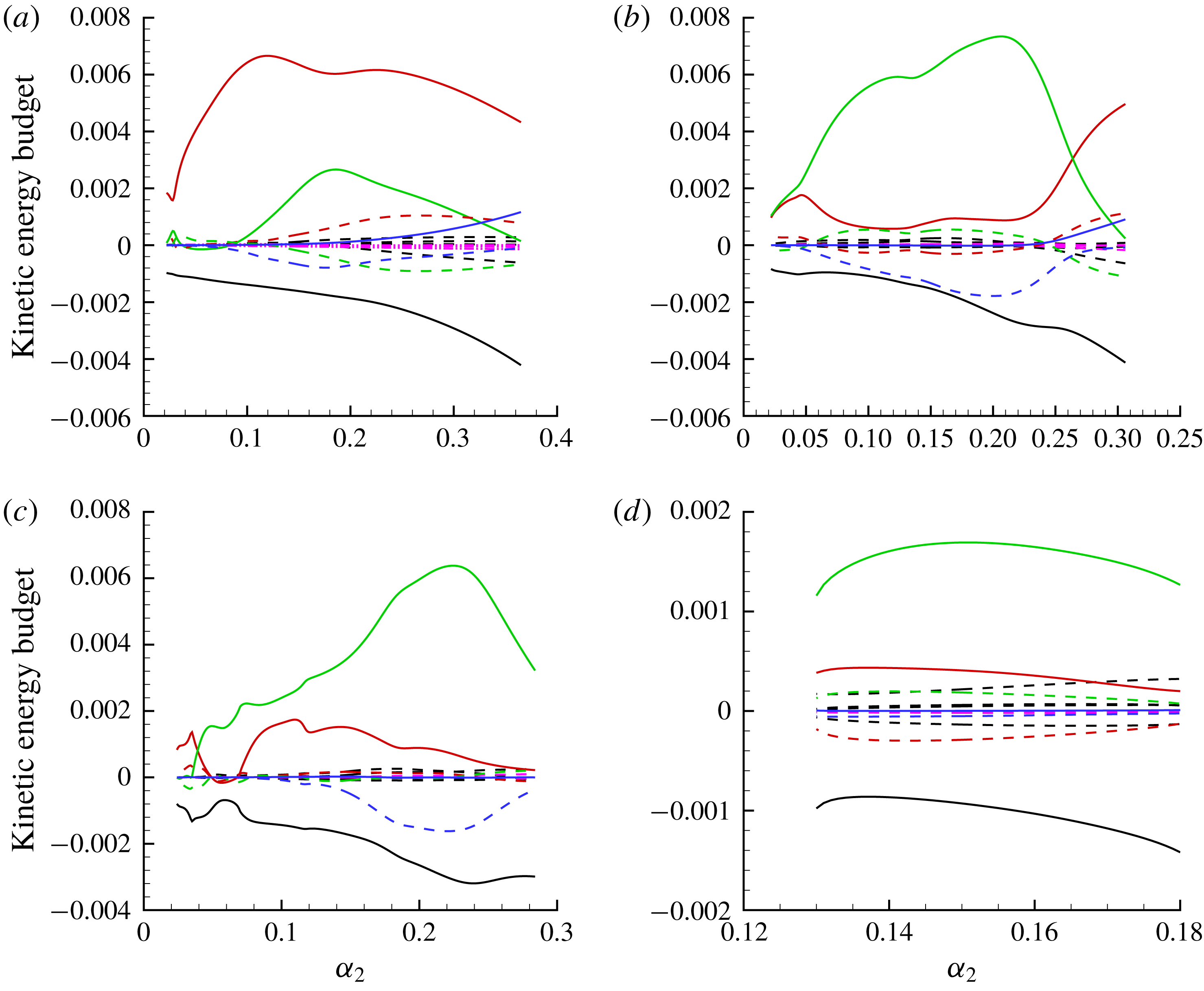
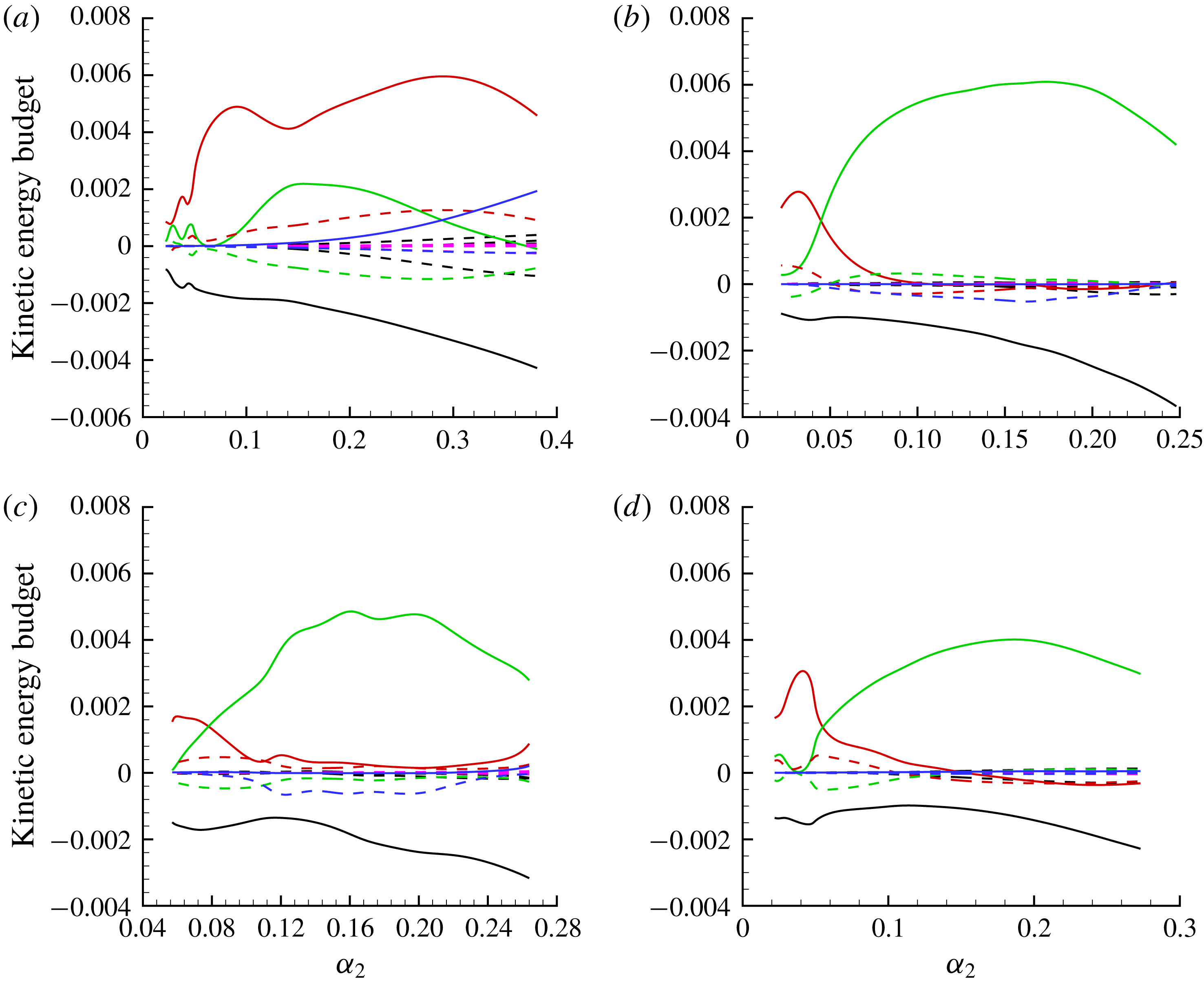
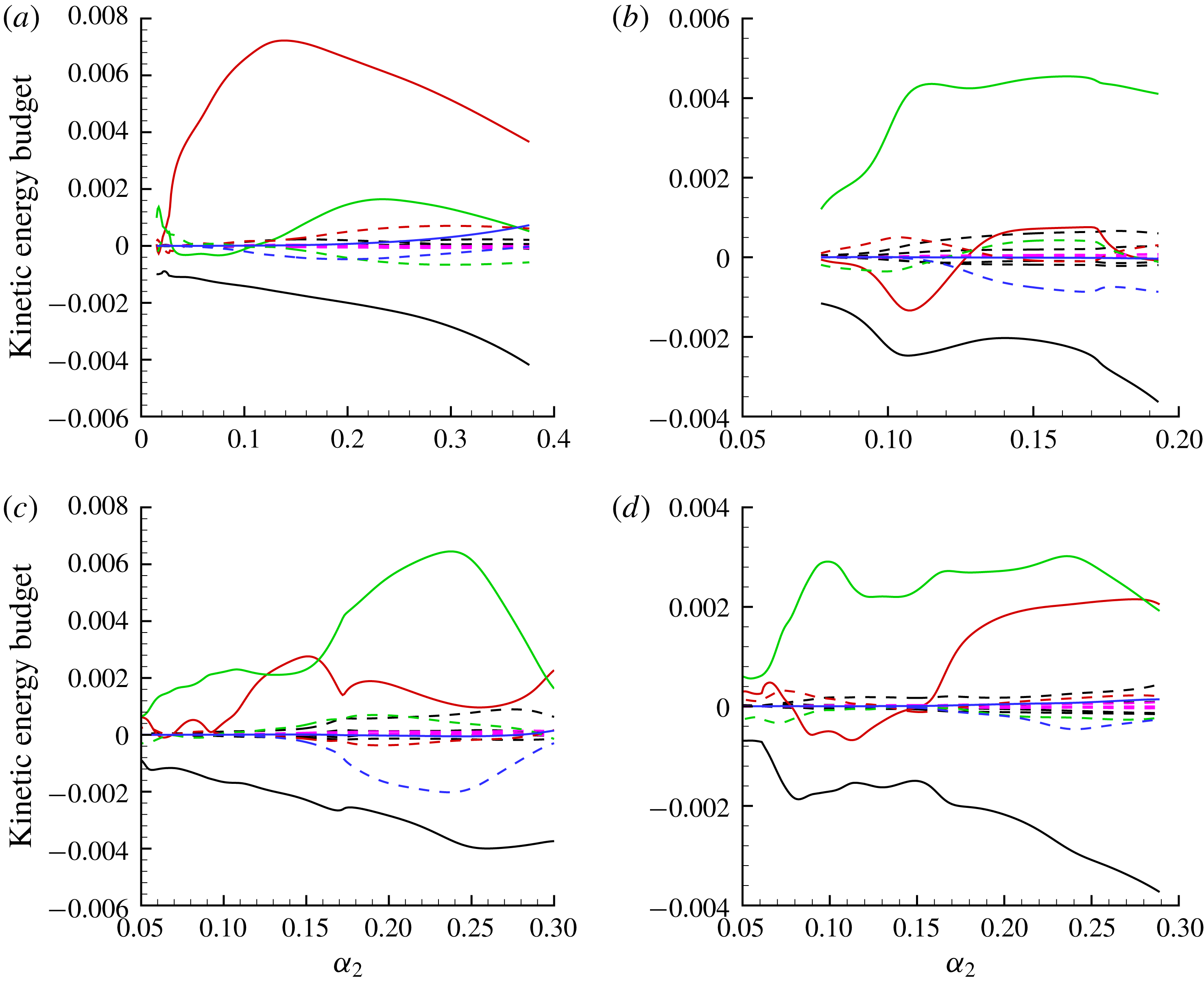
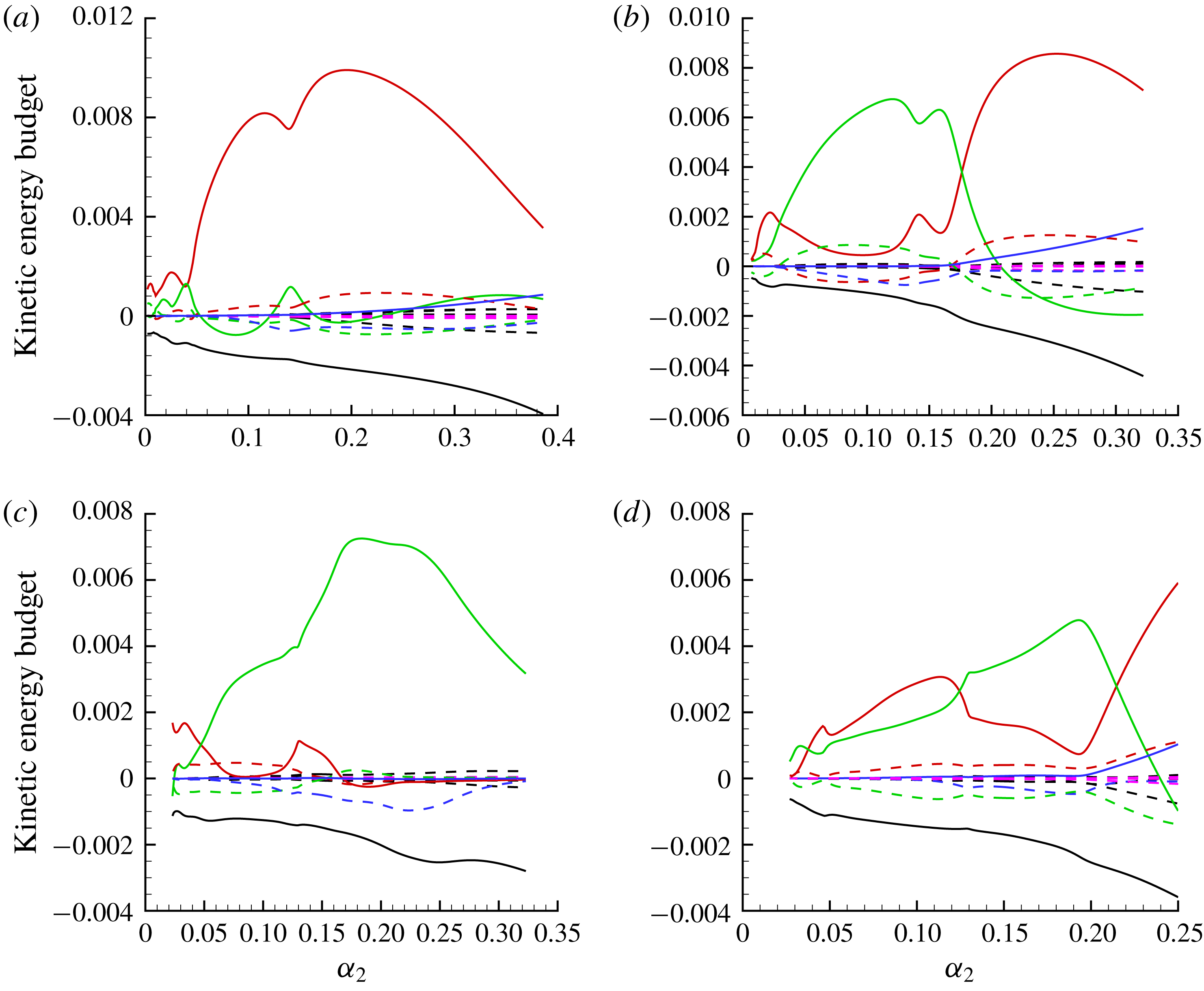
denotes the viscous dissipation and diffusion term. Four secondary instability modes, labelled as modes I, II, III and IV as shown in figures 12(a) and 12(d) and figures 15(a) and 15(d), respectively, are adopted herein for the balance analysis. Mode I stands for the ‘z’ mode, modes II and III the new ‘y’ mode and mode IV the traditional ‘y’ mode.
Kinetic energy budget analyses for (a) mode I (‘z’ mode), (b) mode II (new ‘y’ mode), (c) mode III (new ‘y’ mode) and (d) mode IV (‘y’ mode) at
 $x^{\ast }=0.208~\text{m}$
with
 $A_{01}=5\times 10^{-5}$
. —— (red),
 $\int _{0}^{2\unicode[STIX]{x03C0}/\unicode[STIX]{x1D6FD}_{2}}\int _{0}^{\infty }\int _{0}^{2\unicode[STIX]{x03C0}/\unicode[STIX]{x1D6FC}_{2}}-\unicode[STIX]{x1D70C}_{2}u_{2}^{\prime }w_{2}^{\prime }\unicode[STIX]{x2202}U_{2}/\unicode[STIX]{x2202}z_{2}\,\text{d}\unicode[STIX]{x1D709}_{2}\,\text{d}\unicode[STIX]{x1D702}_{2}\,\text{d}z_{2}$
; —— (green),
 $\int _{0}^{2\unicode[STIX]{x03C0}/\unicode[STIX]{x1D6FD}_{2}}\int _{0}^{\infty }\int _{0}^{2\unicode[STIX]{x03C0}/\unicode[STIX]{x1D6FC}_{2}}-\unicode[STIX]{x1D70C}_{2}u_{2}^{\prime }\unicode[STIX]{x1D710}_{2}^{\prime }\unicode[STIX]{x2202}U_{2}/\unicode[STIX]{x2202}\unicode[STIX]{x1D702}_{2}\,\text{d}\unicode[STIX]{x1D709}_{2}\,\text{d}\unicode[STIX]{x1D702}_{2}\,\text{d}z_{2}$
; – – – (black), the rest of the production terms; – – – (red),
 $\int _{0}^{2\unicode[STIX]{x03C0}/\unicode[STIX]{x1D6FD}_{2}}\int _{0}^{\infty }\int _{0}^{2\unicode[STIX]{x03C0}/\unicode[STIX]{x1D6FC}_{2}}-\unicode[STIX]{x1D70C}_{2}^{\prime }u_{2}^{\prime }W_{2}\unicode[STIX]{x2202}U_{2}/\unicode[STIX]{x2202}z_{2}\,\text{d}\unicode[STIX]{x1D709}_{2}\,\text{d}\unicode[STIX]{x1D702}_{2}\,\text{d}z_{2}$
; – – – (green),
 $\int _{0}^{2\unicode[STIX]{x03C0}/\unicode[STIX]{x1D6FD}_{2}}\int _{0}^{\infty }\int _{0}^{2\unicode[STIX]{x03C0}/\unicode[STIX]{x1D6FC}_{2}}-\unicode[STIX]{x1D70C}_{2}^{\prime }u_{2}^{\prime }V_{2}\unicode[STIX]{x2202}U_{2}/\unicode[STIX]{x2202}\unicode[STIX]{x1D702}_{2}\,\text{d}\unicode[STIX]{x1D709}_{2}\,\text{d}\unicode[STIX]{x1D702}_{2}\,\text{d}z_{2}$
; – – – (purple), the rest of
 $\unicode[STIX]{x1D6EF}_{ij}$
; —— (blue), pressure diffusion term; – – – (blue), pressure dilatation term; —— (black),
 $\unicode[STIX]{x1D700}$
. All terms are scaled by the kinetic energy
 $E_{k}$
.

Kinetic energy budget analyses for (a) mode I (‘z’ mode), (b) mode II (new ‘y’ mode), (c) mode III (new ‘y’ mode) and (d) mode IV (‘y’ mode) at
 $x^{\ast }=0.24~\text{m}$
with
 $A_{01}=5\times 10^{-5}$
. —— (red),
 $\int _{0}^{2\unicode[STIX]{x03C0}/\unicode[STIX]{x1D6FD}_{2}}\int _{0}^{\infty }\int _{0}^{2\unicode[STIX]{x03C0}/\unicode[STIX]{x1D6FC}_{2}}-\unicode[STIX]{x1D70C}_{2}u_{2}^{\prime }w_{2}^{\prime }\unicode[STIX]{x2202}U_{2}/\unicode[STIX]{x2202}z_{2}\,\text{d}\unicode[STIX]{x1D709}_{2}\,\text{d}\unicode[STIX]{x1D702}_{2}\,\text{d}z_{2}$
; —— (green),
 $\int _{0}^{2\unicode[STIX]{x03C0}/\unicode[STIX]{x1D6FD}_{2}}\int _{0}^{\infty }\int _{0}^{2\unicode[STIX]{x03C0}/\unicode[STIX]{x1D6FC}_{2}}-\unicode[STIX]{x1D70C}_{2}u_{2}^{\prime }\unicode[STIX]{x1D710}_{2}^{\prime }\unicode[STIX]{x2202}U_{2}/\unicode[STIX]{x2202}\unicode[STIX]{x1D702}_{2}\,\text{d}\unicode[STIX]{x1D709}_{2}\,\text{d}\unicode[STIX]{x1D702}_{2}\,\text{d}z_{2}$
; – – – (black), the rest of the production terms; – – – (red),
 $\int _{0}^{2\unicode[STIX]{x03C0}/\unicode[STIX]{x1D6FD}_{2}}\int _{0}^{\infty }\int _{0}^{2\unicode[STIX]{x03C0}/\unicode[STIX]{x1D6FC}_{2}}-\unicode[STIX]{x1D70C}_{2}^{\prime }u_{2}^{\prime }W_{2}\unicode[STIX]{x2202}U_{2}/\unicode[STIX]{x2202}z_{2}\,\text{d}\unicode[STIX]{x1D709}_{2}\,\text{d}\unicode[STIX]{x1D702}_{2}\,\text{d}z_{2}$
; – – – (green),
 $\int _{0}^{2\unicode[STIX]{x03C0}/\unicode[STIX]{x1D6FD}_{2}}\int _{0}^{\infty }\int _{0}^{2\unicode[STIX]{x03C0}/\unicode[STIX]{x1D6FC}_{2}}-\unicode[STIX]{x1D70C}_{2}^{\prime }u_{2}^{\prime }V_{2}\unicode[STIX]{x2202}U_{2}/\unicode[STIX]{x2202}\unicode[STIX]{x1D702}_{2}\,\text{d}\unicode[STIX]{x1D709}_{2}\,\text{d}\unicode[STIX]{x1D702}_{2}\,\text{d}z_{2}$
; – – – (purple), the rest of
 $\unicode[STIX]{x1D6EF}_{ij}$
; —— (blue), pressure diffusion term; – – – (blue), pressure dilatation term; —— (black),
 $\unicode[STIX]{x1D700}$
. All terms are scaled by the kinetic energy
 $E_{k}$
.

Kinetic energy budget analyses for (a) mode I (‘z’ mode), (b) mode II (new ‘y’ mode), (c) mode III (new ‘y’ mode) and (d) mode IV (‘y’ mode) at
 $x^{\ast }=0.178~\text{m}$
with
 $A_{01}=1\times 10^{-4}$
. —— (red),
 $\int _{0}^{2\unicode[STIX]{x03C0}/\unicode[STIX]{x1D6FD}_{2}}\int _{0}^{\infty }\int _{0}^{2\unicode[STIX]{x03C0}/\unicode[STIX]{x1D6FC}_{2}}-\unicode[STIX]{x1D70C}_{2}u_{2}^{\prime }w_{2}^{\prime }\unicode[STIX]{x2202}U_{2}/\unicode[STIX]{x2202}z_{2}\,\text{d}\unicode[STIX]{x1D709}_{2}\,\text{d}\unicode[STIX]{x1D702}_{2}\,\text{d}z_{2}$
; —— (green),
 $\int _{0}^{2\unicode[STIX]{x03C0}/\unicode[STIX]{x1D6FD}_{2}}\int _{0}^{\infty }\int _{0}^{2\unicode[STIX]{x03C0}/\unicode[STIX]{x1D6FC}_{2}}-\unicode[STIX]{x1D70C}_{2}u_{2}^{\prime }\unicode[STIX]{x1D710}_{2}^{\prime }\unicode[STIX]{x2202}U_{2}/\unicode[STIX]{x2202}\unicode[STIX]{x1D702}_{2}\,\text{d}\unicode[STIX]{x1D709}_{2}\,\text{d}\unicode[STIX]{x1D702}_{2}\,\text{d}z_{2}$
; – – – (black), the rest of the production terms; – – – (red),
 $\int _{0}^{2\unicode[STIX]{x03C0}/\unicode[STIX]{x1D6FD}_{2}}\int _{0}^{\infty }\int _{0}^{2\unicode[STIX]{x03C0}/\unicode[STIX]{x1D6FC}_{2}}-\unicode[STIX]{x1D70C}_{2}^{\prime }u_{2}^{\prime }W_{2}\unicode[STIX]{x2202}U_{2}/\unicode[STIX]{x2202}z_{2}\,\text{d}\unicode[STIX]{x1D709}_{2}\,\text{d}\unicode[STIX]{x1D702}_{2}\,\text{d}z_{2}$
; – – – (green),
 $\int _{0}^{2\unicode[STIX]{x03C0}/\unicode[STIX]{x1D6FD}_{2}}\int _{0}^{\infty }\int _{0}^{2\unicode[STIX]{x03C0}/\unicode[STIX]{x1D6FC}_{2}}-\unicode[STIX]{x1D70C}_{2}^{\prime }u_{2}^{\prime }V_{2}\unicode[STIX]{x2202}U_{2}/\unicode[STIX]{x2202}\unicode[STIX]{x1D702}_{2}\,\text{d}\unicode[STIX]{x1D709}_{2}\,\text{d}\unicode[STIX]{x1D702}_{2}\,\text{d}z_{2}$
; – – – (purple), the rest of
 $\unicode[STIX]{x1D6EF}_{ij}$
; —— (blue), pressure diffusion term; – – – (blue), pressure dilatation term; —— (black),
 $\unicode[STIX]{x1D700}$
. All terms are scaled by the kinetic energy
 $E_{k}$
.

Kinetic energy budget analyses for (a) mode I (‘z’ mode), (b) mode II (new ‘y’ mode), (c) mode III (new ‘y’ mode) and (d) mode IV (‘y’ mode) at
 $x^{\ast }=0.208~\text{m}$
with
 $A_{01}=1\times 10^{-4}$
. —— (red),
 $\int _{0}^{2\unicode[STIX]{x03C0}/\unicode[STIX]{x1D6FD}_{2}}\int _{0}^{\infty }\int _{0}^{2\unicode[STIX]{x03C0}/\unicode[STIX]{x1D6FC}_{2}}-\unicode[STIX]{x1D70C}_{2}u_{2}^{\prime }w_{2}^{\prime }\unicode[STIX]{x2202}U_{2}/\unicode[STIX]{x2202}z_{2}\,\text{d}\unicode[STIX]{x1D709}_{2}\,\text{d}\unicode[STIX]{x1D702}_{2}\,\text{d}z_{2}$
; —— (green),
 $\int _{0}^{2\unicode[STIX]{x03C0}/\unicode[STIX]{x1D6FD}_{2}}\int _{0}^{\infty }\int _{0}^{2\unicode[STIX]{x03C0}/\unicode[STIX]{x1D6FC}_{2}}-\unicode[STIX]{x1D70C}_{2}u_{2}^{\prime }\unicode[STIX]{x1D710}_{2}^{\prime }\unicode[STIX]{x2202}U_{2}/\unicode[STIX]{x2202}\unicode[STIX]{x1D702}_{2}\,\text{d}\unicode[STIX]{x1D709}_{2}\,\text{d}\unicode[STIX]{x1D702}_{2}\,\text{d}z_{2}$
; – – – (black), the rest of the production terms; – – – (red),
 $\int _{0}^{2\unicode[STIX]{x03C0}/\unicode[STIX]{x1D6FD}_{2}}\int _{0}^{\infty }\int _{0}^{2\unicode[STIX]{x03C0}/\unicode[STIX]{x1D6FC}_{2}}-\unicode[STIX]{x1D70C}_{2}^{\prime }u_{2}^{\prime }W_{2}\unicode[STIX]{x2202}U_{2}/\unicode[STIX]{x2202}z_{2}\,\text{d}\unicode[STIX]{x1D709}_{2}\,\text{d}\unicode[STIX]{x1D702}_{2}\,\text{d}z_{2}$
; – – – (green),
 $\int _{0}^{2\unicode[STIX]{x03C0}/\unicode[STIX]{x1D6FD}_{2}}\int _{0}^{\infty }\int _{0}^{2\unicode[STIX]{x03C0}/\unicode[STIX]{x1D6FC}_{2}}-\unicode[STIX]{x1D70C}_{2}^{\prime }u_{2}^{\prime }V_{2}\unicode[STIX]{x2202}U_{2}/\unicode[STIX]{x2202}\unicode[STIX]{x1D702}_{2}\,\text{d}\unicode[STIX]{x1D709}_{2}\,\text{d}\unicode[STIX]{x1D702}_{2}\,\text{d}z_{2}$
; – – – (purple), the rest of
 $\unicode[STIX]{x1D6EF}_{ij}$
; —— (blue), pressure diffusion term; – – – (blue), pressure dilatation term; —— (black),
 $\unicode[STIX]{x1D700}$
. All terms are scaled by the kinetic energy
 $E_{k}$
.

For the case with
 $A_{01}=5\times 10^{-5}$
, figures 18 and 19 show the contributions of the production, advection, diffusion and dissipation terms to the growth rates of these four secondary instability modes of the stationary cross-flow vortex at
 $x^{\ast }=0.208~\text{m}$
and 0.24 m, respectively. As shown in figures 18(a) and 19(a) for mode I of the ‘z’ mode, it can be concluded that the integrated production term
 $-\unicode[STIX]{x1D70C}_{2}u_{2}^{\prime }w_{2}^{\prime }\unicode[STIX]{x2202}U_{2}/\unicode[STIX]{x2202}z_{2}$
of spanwise shear dominates. For the non-parallel terms
 $\unicode[STIX]{x1D6EF}_{ij}$
, the terms
 $-\unicode[STIX]{x1D70C}_{2}^{\prime }u_{2}^{\prime }W_{2}\unicode[STIX]{x2202}U_{2}/\unicode[STIX]{x2202}z_{2}$
and
 $-\unicode[STIX]{x1D70C}_{2}^{\prime }u_{2}^{\prime }V_{2}\unicode[STIX]{x2202}U_{2}/\unicode[STIX]{x2202}\unicode[STIX]{x1D702}_{2}$
corresponding to the spanwise shear and wall-normal shear are also dominant, but the rest of the non-parallel terms are very small. However, the magnitudes of the terms
 $-\unicode[STIX]{x1D70C}_{2}^{\prime }u_{2}^{\prime }W_{2}\unicode[STIX]{x2202}U_{2}/\unicode[STIX]{x2202}z_{2}$
and
 $-\unicode[STIX]{x1D70C}_{2}^{\prime }u_{2}^{\prime }V_{2}\unicode[STIX]{x2202}U_{2}/\unicode[STIX]{x2202}\unicode[STIX]{x1D702}_{2}$
are almost equal but with opposite signs. Thereby, it can be concluded that the non-parallel term
 $\unicode[STIX]{x1D6EF}$
has little influence on the growth rate of the ‘z’ mode. Furthermore, the role of the pressure fluctuation term including the pressure diffusion and pressure dilatation in the energy production of secondary instability modes is also investigated to account for the effect of compressibility. In fact, for the compressible mixing layer flow, Vreman, Sandham & Luo (Reference Vreman, Sandham and Luo1996) had shown that the spatial distribution of the pressure field will be changed due to the effect of compressibility. In the study of hypersonic turbulent boundary layer flow, Duan, Beekman & Martin (Reference Duan, Beekman and Martin2011) using DNS showed that the pressure diffusion term was large and positive near the wall, but the pressure dilatation arising from non-vanishing velocity divergence was very small and negative. Nevertheless, for the ‘z’ mode, the pressure diffusion term
 $D_{iff}$
is also always positive but only prompts the growth rate of the ‘z’ mode with higher streamwise wavenumber (higher frequency). The pressure dilatation term
 $\unicode[STIX]{x1D6F1}$
is always negative and cannot be ignored. The dissipation term
 $\unicode[STIX]{x1D700}$
accounts for the effect of viscosity, it can be seen that the dissipation term is always negative. Also, the magnitude of the dissipation term
 $\unicode[STIX]{x1D700}$
will increase with increasing streamwise wavenumber of the secondary instability modes.
When considering figures 18(b,c) and 19(b,c) together for mode II and III of the new ‘y’ mode, it is obvious that the term
 $-\unicode[STIX]{x1D70C}_{2}u_{2}^{\prime }\unicode[STIX]{x1D710}_{2}^{\prime }\unicode[STIX]{x2202}U_{2}/\unicode[STIX]{x2202}\unicode[STIX]{x1D702}_{2}$
plays a central role in the energy production
 $P_{k}$
, justifying that it belongs to the class of ‘y’ mode. The role of non-parallel terms
 $\unicode[STIX]{x1D6EF}$
in the growth rate of the new ‘y’ mode can also be ignored. However, the pressure diffusion term
 $D_{iff}$
has little influence on energy transfer. Nevertheless, the pressure dilatation term
 $\unicode[STIX]{x1D6F1}$
subjected to the non-vanishing velocity divergence will significantly hinder the growth rate of the new ‘y’ mode. For the traditional ‘y’ mode as shown in both figures 18(d) and 19(d), the trends of the various production terms in the growth rate are seen to be roughly the same for those of the new ‘y’ mode.
In what follows, the energy budget for the case with
 $A_{01}=10^{-4}$
is considered. Figure 20 shows the contributions of various production terms to the growth rates of these four secondary instability modes at
 $x^{\ast }=0.178~\text{m}$
. The role of the production terms is generally consistent with the previous case. Figure 21 shows the same results for modes I, II, III and IV at
 $x^{\ast }=0.208~\text{m}$
. According to figure 21(a), the mode I is a ‘z’ mode. As shown in figure 17(b), mode II with
 $\unicode[STIX]{x1D6FC}_{2}=0.14$
is a new ‘y’ mode. Figure 21(b) shows that the dominant production is
 $-\unicode[STIX]{x1D70C}_{2}u_{2}^{\prime }\unicode[STIX]{x1D710}_{2}^{\prime }\unicode[STIX]{x2202}U_{2}/\unicode[STIX]{x2202}\unicode[STIX]{x1D702}_{2}$
for mode II with
 $0<\unicode[STIX]{x1D6FC}_{2}<0.18$
. Whereas it can also be inferred that mode II with
 $0.18<\unicode[STIX]{x1D6FC}_{2}<0.32$
will be the ‘z’ mode as the spanwise shear term
 $-\unicode[STIX]{x1D70C}_{2}u_{2}^{\prime }w_{2}^{\prime }\unicode[STIX]{x2202}U_{2}/\unicode[STIX]{x2202}z_{2}$
is dominant. In order to further shed light on the characteristic of mode II at
 $x^{\ast }=0.208~\text{m}$
, the mode shapes of mode II with
 $\unicode[STIX]{x1D6FC}_{2}=0.12$
and
 $\unicode[STIX]{x1D6FC}_{2}=0.25$
at
 $x^{\ast }=0.208~\text{m}$
, corresponding to the maximum of wall-normal shear and spanwise shear, are shown in figures 22(a) and 22(b) respectively. Thereby, it can be seen that mode II with
 $\unicode[STIX]{x1D6FC}_{2}=0.12$
belongs to the class of new ‘y’ mode, while mode II with
 $\unicode[STIX]{x1D6FC}_{2}=0.25$
is the ‘z’ mode. Furthermore, when the spanwise shear term dominates the energy production of the mode II with
 $0.18<\unicode[STIX]{x1D6FC}_{2}<0.32$
, the importance of the pressure diffusion term
 $D_{iff}$
increases, as with the genuine ‘z’ mode. It is further concluded that the pressure diffusion term
 $D_{iff}$
will significantly enhance the growth rate of the ‘z’ mode with higher streamwise wavenumber as mentioned above. As mentioned in the previous section, mode IV at
 $x^{\ast }=0.208~\text{m}$
is a mixed ‘y’/‘z’ mode, since its velocity fluctuation is concentrated at both the top and shoulder of the stationary cross-flow vortex. It can also be justified from figure 21(d) that the importance of the production terms
 $-\unicode[STIX]{x1D70C}_{2}u_{2}^{\prime }\unicode[STIX]{x1D710}_{2}^{\prime }\unicode[STIX]{x2202}U_{2}/\unicode[STIX]{x2202}\unicode[STIX]{x1D702}_{2}$
and
 $-\unicode[STIX]{x1D70C}_{2}u_{2}^{\prime }w_{2}^{\prime }\unicode[STIX]{x2202}U_{2}/\unicode[STIX]{x2202}z_{2}$
is comparable.
(a) The
 $|u_{2}^{\prime }|$
-eigenfunction of mode II with
 $\unicode[STIX]{x1D6FC}_{2}=0.12$
; (b) the
 $|u_{2}^{\prime }|$
-eigenfunction of mode II with
 $\unicode[STIX]{x1D6FC}_{2}=0.25$
for
 $A_{01}=10^{-4}$
at
 $x^{\ast }=0.208~\text{m}$
. White dash lines represent the stationary cross-flow vortex.

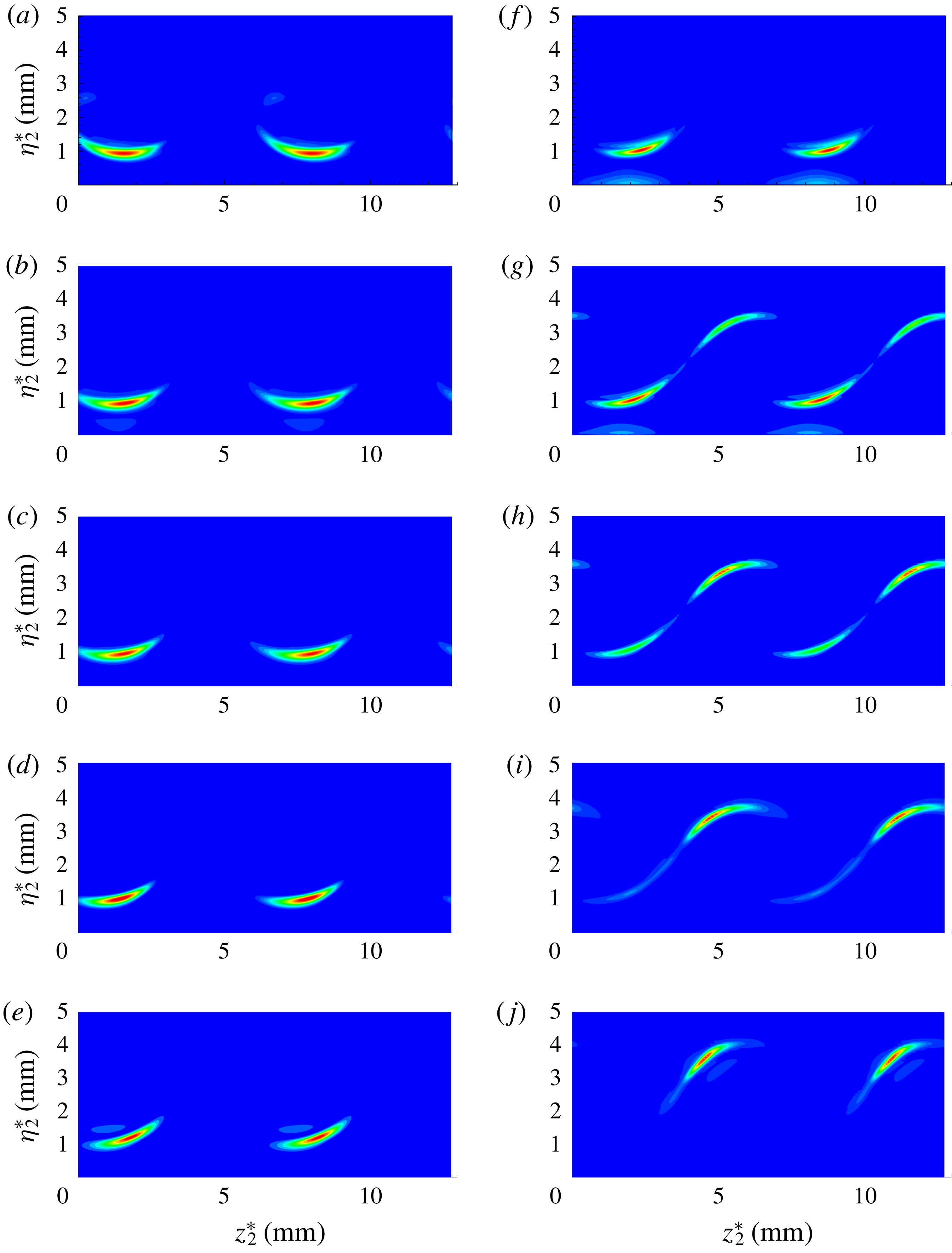
Downstream evolution of the
 $|\unicode[STIX]{x1D70C}_{2}^{\prime }u_{2}^{\prime }|$
-eigenfunction of secondary instability modes as a function of chordwise position
 $x^{\ast }$
. (a)
 $x^{\ast }=0.178~\text{m}$
, (b)
 $x^{\ast }=0.1825~\text{m}$
, (c)
 $x^{\ast }=0.185~\text{m}$
, (d)
 $x^{\ast }=0.190~\text{m}$
, (e)
 $x^{\ast }=0.208~\text{m}$
for the new ‘y’ mode with
 $\unicode[STIX]{x1D714}_{2}=0.089$
; and (f)
 $x^{\ast }=0.178~\text{m}$
, (g)
 $x^{\ast }=0.1825~\text{m}$
, (h)
 $x^{\ast }=0.185~\text{m}$
, (i)
 $x^{\ast }=0.190~\text{m}$
and (j)
 $x^{\ast }=0.208~\text{m}$
for the new ‘y’ mode with
 $\unicode[STIX]{x1D714}_{2}=0.193$
.

In particular, Malik et al. (Reference Malik, Li, Choudhari and Chang1999) had shown that the wall-normal shear reduces the energy production of the ‘z’ mode, and the spanwise shear decreases the growth rate of the ‘y’ mode (figure 9 in Malik et al. (Reference Malik, Li, Choudhari and Chang1999)). However, for the secondary cross-flow instability in the hypersonic three-dimensional boundary layer of the present study, it is shown that the wall-normal shear can actually support the energy production of the ‘z’ mode, and the spanwise shear can also enhance the growth rate of the ‘y’ mode. This indicates that the ‘y’ and ‘z’ modes can be exchanged. As mentioned above, mode II with
 $\unicode[STIX]{x1D6FC}_{2}=0.12$
is a new ‘y’ mode and mode II with
 $\unicode[STIX]{x1D6FC}_{2}=0.25$
is a ‘z’ mode at
 $x^{\ast }=0.208~\text{m}$
. Mode II at
 $x^{\ast }=0.178~\text{m}$
is always a new ‘y’ mode according to figure 20(b). It is inferred here that the new ‘y’ mode of mode II with higher streamwise wavenumber (higher frequency) can evolve into a ‘z’ mode in the downstream region.
In order to justify this mode switching, mode II with
 $\unicode[STIX]{x1D6FC}_{2}=0.12,0.25$
at
 $x^{\ast }=0.208~\text{m}$
is traced back along the upstream using spatial secondary instability theory. To achieve this upstream tracing, the temporal secondary instability modes of mode II at
 $x^{\ast }=0.208~\text{m}$
are changed into the spatial secondary instability mode by using the Arnoldi method; fixing the imaginary part of the complex frequency
 $\unicode[STIX]{x1D714}_{2}$
and increasing the imaginary part of the streamwise wavenumber
 $\unicode[STIX]{x1D6FC}_{2}$
until the real part of
 $\unicode[STIX]{x1D714}_{2}$
became smaller than
 $10^{-7}$
. The spatial secondary instability mode obtained from the previous step is selected as the initial condition, and is then traced upstream by solving the eigenvalue problem with inverse Rayleigh iteration. The upstream evolutions of
 $|\unicode[STIX]{x1D70C}_{2}^{\prime }u_{2}^{\prime }|$
of mode II with
 $\unicode[STIX]{x1D6FC}_{2}=0.12$
(
 $\unicode[STIX]{x1D714}_{2}=0.089$
) are shown in figure 23(a–e). The characteristic of mode II with
 $\unicode[STIX]{x1D6FC}_{2}=0.12$
(
 $\unicode[STIX]{x1D714}_{2}=0.089$
) is independent of the chordwise position, indicating that it always belongs to the type of new ‘y’ mode. Also, figure 23(f–j) shows the upstream developments of
 $|\unicode[STIX]{x1D70C}_{2}^{\prime }u_{2}^{\prime }|$
of mode II with
 $\unicode[STIX]{x1D6FC}_{2}=0.25$
(
 $\unicode[STIX]{x1D714}_{2}=0.193$
). It is seen there that mode II with
 $\unicode[STIX]{x1D6FC}_{2}=0.25$
(
 $\unicode[STIX]{x1D714}_{2}=0.193$
) at
 $x^{\ast }=0.208~\text{m}$
is a ‘z’ mode but changes into a new ‘y’ mode at
 $x^{\ast }=0.178~\text{m}$
. Thus, it can be concluded that the new ‘y’ mode with higher streamwise wavenumber (higher frequency) evolves into the ‘z’ mode as the flow moves downstream.
In the recent experiment of Craig & Saric (Reference Craig and Saric2016), no ‘y’ mode had been observed. They argued that the frequency of the ‘y’ mode was expected to be outside the range of the measurement system. However, high-frequency fluctuations of the ‘z’ mode with frequency in the range of [80–130] kHz were observed at
 $x^{\ast }=350~\text{mm}$
, and parts of its velocity disturbance were also concentrated at the trough of the stationary cross-flow vortex (figure 8b in Craig & Saric (Reference Craig and Saric2015) or figure 9 in Craig & Saric (Reference Craig and Saric2016)). The mode shape of the ‘z’ mode at
 $x^{\ast }=350~\text{mm}$
appears rather similar to the mode shape of figure 23(g) in the present work. Also, the velocity disturbances concentrated at the trough of the stationary cross-flow vortex of the ‘z’ mode at
 $x^{\ast }=350~\text{mm}$
decayed downstream and only the ‘z’ mode could be observed at further downstream locations until
 $x^{\ast }=390~\text{mm}$
(figure 9 in Craig & Saric (Reference Craig and Saric2016)). This is consistent with the present study, that the new ‘y’ mode can evolve into the ‘z’ mode in the downstream.
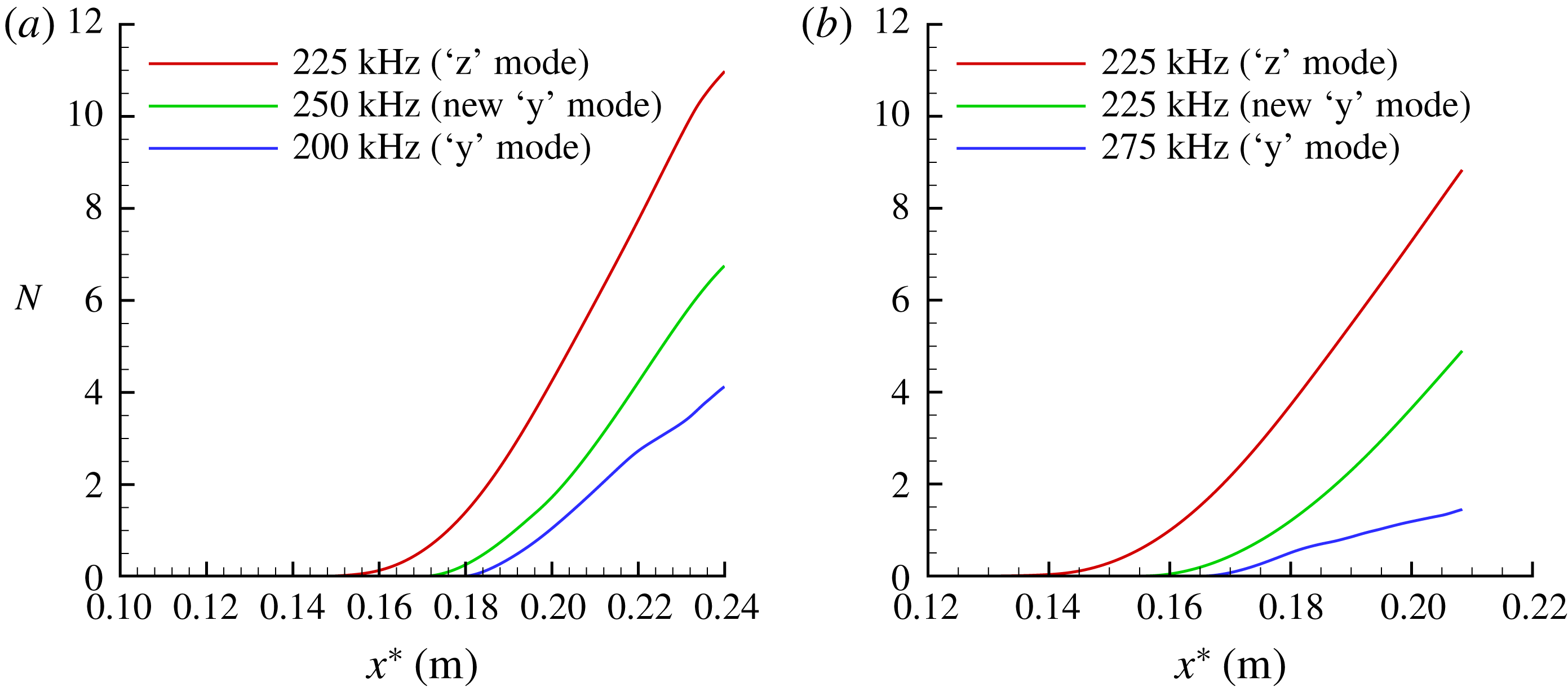
Figure 24(a,b) also shows the
 $N$
-factor results of high-frequency modes for these two cases by using spatial secondary instability theory. There is no doubt that the most amplified secondary instability mode is the ‘z’ mode in the current analysis, the
 $N$
factor for the new ‘y’ mode is moderately lower, and the frequencies corresponding to the most amplified ‘z’ mode and new ‘y’ mode are comparable. Throughout the chordwise range, the traditional ‘y’ mode grows slowly. This may be the reason why the traditional ‘y’ mode on top of the stationary cross-flow vortex was not observed in Craig & Saric (Reference Craig and Saric2016) experiment.
The
 $N$
-factor results of the most amplified high-frequency modes for cases: (a)
 $A_{01}=5\times 10^{-5}$
, (b)
 $A_{01}=1\times 10^{-4}$
.

5 Conclusions
A Floquet analysis has been carried out to investigate the secondary instabilities of stationary cross-flow vortices in a Mach 6.0 swept wing boundary layer flow. The high-frequency ‘z’ mode and ‘y’ mode of secondary instability modes defined in low-speed swept wing flow are first observed. The behaviours of these secondary instability modes are consistent with low-speed cases in that the ‘z’ mode is located on the shoulder of the stationary cross-flow vortex and the ‘y’ mode appears at the crest. An important finding of the present study is that a new type of secondary instability mode is excited at the trough of the stationary cross-flow vortex under the present hypersonic condition. It is confirmed that this new type secondary instability mode belongs to the class of ‘y’ mode based on the balance analysis of the disturbance kinetic energy. In fact, in a study of the hypersonic flow over a cone pitched at
 $6^{\circ }$
angle of attack, Li et al. (Reference Li, Choudhari, Paredes and Duan2016) showed that the velocity fluctuations of the Mack mode were concentrated at the trough of the stationary cross-flow vortex when the laminar flow had been modified by the stationary cross-flow vortex (figure 13 in Li et al. (Reference Li, Choudhari, Paredes and Duan2016)). This indicates that the high shear layer corresponding to the maximum wall-normal gradient at the trough of the stationary cross-flow vortex can support the secondary cross-flow instability. The N-factors show that the ‘z’ mode is the most amplified high-frequency mode, and that the new ‘y’ mode is substantially more unstable than the traditional ‘y’ mode on top of the stationary cross-flow vortex. This indicates that the traditional ‘y’ mode at the crest of the stationary cross-flow vortex is not necessarily the most important in the hypersonic three-dimensional boundary layer flow.
The role of the pressure fluctuation term, including the pressure diffusion and pressure dilatation, in the energy production of cross-flow secondary instability modes is also investigated through the kinetic energy balance analysis. It is found that the pressure diffusion will only enhance the growth rate of the ‘z’ mode with higher frequency, and the pressure dilatation term arising from non-vanishing velocity divergence will reduce the growth rates of all secondary instability modes. It is numerically shown that the new ‘y’ mode can evolve into the ‘z’ mode in the downstream. Thus, more research attention should be paid to understanding the role of this new ‘y’ mode in hypersonic cross-flow instabilities.
Acknowledgements
This paper is supported by the National Key Research and Development Program of China (2016YFA0401200) and the National Science Foundation of China under Contract 11302245, 11702307 and 11572176.