1. INTRODUCTION
It has been known for some time that in certain parametric regression models it is possible to “adapt” to an unknown error distribution by maximizing an estimated likelihood function based on an estimate of the error distribution. The common result is that you do as well in terms of the asymptotic variance of the estimated parameters as if you knew the true error distribution, hence the term adaptive. In estimation problems where a Gaussian assumption on the underlying distribution of the data is inappropriate, adaptive estimation provides an alternative to the conventional Gaussian maximum likelihood estimator by replacing the Gaussian density function with a nonparametric estimate of the score function of the log-likelihood. It has been proved that an efficiency gain over the least squares methods can be achieved by adaptive estimators in many models.
Adaptive estimation was first studied by Stein (1956), who considered the problem of estimating and testing hypotheses about a parameter in the presence of an infinite-dimensional “nuisance” parameter. Beran (1974) and Stone (1975) considered adaptive estimation in the symmetric location model, and Bickel (1982) extended this to linear regression and other models. This latter work provided a starting point for much future work in this area, most of which has exploited the property of local asymptotic normality (LAN) of the class of likelihoods involved. Manski (1984) studied adaptive estimation in nonlinear models, Kreiss (1987) considered stationary and invertible autoregressive moving average (ARMA) models, Steigerwald (1992) studied linear regression with ARMA error, and Linton (1993) considered the case of linear regression with autoregressive conditional heteroskedasticity (ARCH), which was extended by Drost and Klaassen (1997) to the GARCH(1,1) case. Jeganathan (1995) extended the theory to nonstationary models with independent and identically distributed (i.i.d.) error, which involves the generalization to local asymptotic mixed normal (LAMN) likelihoods. Hodgson (1998a, 1998b) further extended this case but with ARMA errors.
All of the preceding literature considers adaptive estimation of the parametric component in semiparametric models.1
One exception is recent work by Zhang and Liu (2003) on local modeling based on empirical likelihood.

where εi is an i.i.d. error term possessing smooth Lebesgue density, is independent of X almost surely, and satisfies E [εi] = 0 and E [|εi|] < ∞. The moment condition is essential to the interpretation of m as the conditional expectation of Yi given Xi, and we shall maintain this assumption throughout. This is somewhat different from the semiparametric literature cited before, e.g., Bickel (1982), where typically no moment conditions are made but some other identifying condition such as symmetric errors is made. The assumption that m is a smooth function implies that for Xi close to x, Yi contains information about m(x). A popular estimator of m(x) is the local polynomial regression estimator, which can also be obtained from the following weighted least squares criterion:

where K is a kernel function, h = h(n) is a bandwidth sequence, and

is a pth-order polynomial of Xi − x with coefficient vector θ. When εi are Gaussian, (2) corresponds to the weighted likelihood criterion. In the absence of Gaussianity, asymptotic results of the preceding estimator generally still hold, but this estimator is less efficient in terms of mean squared error (MSE) than estimators that exploit the distributional information. If the error density f were known, we could replace

in (2) by the log-likelihood

and obtain a likelihood-based estimator (Fan, Farmen, and Gijbels, 1998). The local likelihood estimator has lower variance than the least-squares-based local polynomial estimator as follows by the classical Cramér–Rao inequality; under some conditions, the bias of the local likelihood estimator is the same as the bias of the simple local polynomial estimator, so that the local likelihood estimator has lower MSE. In the conventional kernel estimation literature, Tibshirani (1984) introduced the local likelihood estimator in the context of nonparametric generalized linear models. This study was extended in Hastie and Tibshirani (1987). Staniswalis (1989) applied this idea to the estimation of a location parameter θ; she also derived the asymptotic variance of her local constant procedure, although she did not give the bias. Also see Hunsberger (1994), Fan, Heckman, and Wand (1995), Aerts and Claeskens (1997), and Carroll, Ruppert, and Welsh (1998) for related studies. There has been much recent work mostly focusing on density and hazard estimation. In particular see Copas (1994), Hjort (1993), Hjort and Jones (1996), and Loader (1996). Work in other areas includes Robinson (1989) for a time series regression problem and the recent paper by Gozalo and Linton (2000) for nonlinear regression models. These procedures are discussed in Härdle and Linton (1994, esp. p. 17).
In practice, f is generally unknown, and the local likelihood estimator is infeasible. We propose an adaptive procedure for the estimation of (1) based on estimating the score function of the errors, i.e., by replacing f by a nonparametric estimator thereof. We establish the pointwise asymptotic distribution of our estimator of m(x), for interior x, and show that it adapts in the sense that it has the same variance as the infeasible procedure based on knowing the error distribution. This is true regardless of the dimensionality of the regressors. A more complicated implementation of our procedure involves undersmoothing at the first step and will result in an estimator with exactly the same bias as the infeasible local likelihood estimator. In this case, our adaptive estimator achieves the same MSE in large samples as the infeasible local likelihood estimator. In this sense, our estimator is efficient. This is not to say that our method has any special properties with regard to minimax risk; as is well known it is not possible to achieve the lower bound here; see Fan (1993). But the pairwise comparison has been used elsewhere; see Linton (1997) and Fan, Härdle, and Mammen (1998). With regard to regularity conditions we make relatively strong assumptions about the smoothness of the regression function and density function but impose very few other requirements on the error distribution other than some minimal moment conditions that are required for the interpretation of our estimand as a regression function and for the good behavior of the benchmark nonparametric regression estimator. In the main set of conditions we allow the error distribution to have unbounded support. We also look at the case of bounded support. In the latter case, we must also require that the error density approaches zero at the boundary rather fast because otherwise the estimation problem is nonregular, i.e., there exist estimators that converge to the true value more rapidly.
Why is this method important in practice? In many data sets the error distribution is likely to be nonnormally distributed and perhaps quite far from the normal distribution to such an extent that the local likelihood estimator has much lower variance than the Gaussian-based estimators (and the relative efficiency is unbounded). As a modeling issue it is hard to believe that we have better information about the error density than about the shape of the main regression effect, and so it is quite natural to treat the error density as an unknown parameter just like the regression function. Thus our results are comforting in that they say that we can still use information from the error distribution to improve the performance of our regression estimates; this is all the more important in nonparametric regression because the rate of convergence can be so slow.
The principle involved extends to allow for heteroskedasticity of unknown form and to other location models that depend on several functional parameters, such as additive regression models. In more general nonparametric models, we may or may not find adaptivity just as in the parametric case; see Bickel, Klaassen, Ritov, and Wellner (1993).
The paper is organized as follows. The model and estimators are given in the next section. The main asymptotic results of the proposed estimator are given in Section 3. In Section 4 we discuss the relaxation of the independence assumption. In Section 5 we provide a small Monte Carlo experiment that evaluates the effectiveness of the adaptive regression estimator. Section 6 concludes, and the Appendix contains the proofs of the main results.
For notation, we use f(j) to denote the jth derivative of a function f. We also let ∥A∥ denote the euclidean norm of the array A = (ai1,…, is) defined as ∥A∥ = ([sum ]ai1,…, is2)1/2. For vectors k = (k1,…, kd) and x = (x1,…, xd), we use the following notation:

2. THE MODEL AND ESTIMATOR
2.1. The Model and an Infeasible Estimator
Suppose that {Yi,Xi}i=1n are i.i.d., where

and

. We consider the regression model (1) where εi is independent of Xi with E(εi) = 0 and εi has a density function f. We are interested in estimation of the regression function

where x is an interior point in the support of Xi and m(·) is assumed to be of unknown form, but smooth. We concentrate on the regression case; instead one could treat other location functionals such as the conditional median, in which case the finite variance we assume in Assumption A1 in Section 3 would not be required. However, it is central to identification that the location functional be explicitly specified as this determines the estimation strategy. In view of this we focus on the regression problem for which finite variance is a common and natural assumption.
The approach proposed in this paper may be applied to a wide range of nonparametric estimators, including the widely used Nadaraya–Watson procedure and the local polynomial estimator. In this paper, we give an asymptotic analysis based on the local polynomial procedures. See Fan (1992) and Fan and Gijbels (1996) for discussion on the attractive properties of local polynomials. For a given data set {Yi,Xi}i=1n, the local polynomial M-estimator of Yi on Xi of order p (where p is an integer) can be obtained from minimizing the following criterion:

where ϱamp; is a user-determined criterion,

is a pth-order polynomial in the vector u with coefficients θ, K(u) is a nonnegative weight function on

, and h is a bandwidth parameter. Let θ be the vector of minimizing parameters in (5) and let m(x) = θ0, where θ0 is the minimizing intercept.
Following the notation of Masry (1996a, 1996b), let N[ell ] = ([ell ] + d − 1)!/[ell ]!(d − 1)! be the number of distinct d-tuples j with | j| = [ell ]. Arrange these N[ell ] d-tuples as a sequence in a lexicographical order and let φ[ell ]−1 denote this one-to-one map. For each j with 0 ≤ | j| ≤ 2p, let

,

, and define the N × N–dimensional matrices M and Γ and N × 1 vector B, where

, by

where Mi,j and Γi,j are Ni × Nj–dimensional matrices whose ([ell ],m) elements are, respectively, μφi([ell ])+φj(m) and νφi([ell ])+φj(m). Note that the elements of the matrices M = M(K) and Γ = Γ(K) are simply multivariate moments of the kernel K and K2, respectively. In addition, we arrange the Nr elements of the derivatives

as a column vector m(r)(x).
In the case that the error density f is known, it is desirable to take ϱamp; ∝ log f in (5), in which case the estimator has a local likelihood interpretation. When εi is normally distributed, ϱamp;(z) = z2, and the resulting m(x) is the standard local polynomial regression smoother, whereas if εi is assumed to be Laplace distributed, then m(x) is the standard local polynomial median smoother; see Chaudhuri (1991).
In general, the estimator m(x) is only implicitly defined and is a nonlinear function of Y1,…,Yn. In practice some numerical algorithm must be used to compute the values θ, such as the Newton–Raphson method. We shall work with the one-step Newton–Raphson estimator (as analyzed in Bickel, 1975, for a class of parametric estimation problems) from a preliminary consistent estimator

(say, the local polynomial least squares estimator that takes ϱamp;(z) = z2 in (5)); i.e., let mNR(x) be the first element of θNR(x), where

where Sn(θ; f) is the smoothed score function

where

and Xi,| j|(x) (0 ≤ |j| ≤ p) is an N| j|-dimensional subvector whose rth element is given by [Xi,| j|]r = (x − Xi)φ| j|(r), whereas

is a consistent estimate of the information

given by

We next state the properties of θ(x) (and thus m(x)). Proposition 1 is essentially Fan and Chen (1999) except that we allow for a more general multivariate random design for the covariates. It gives the asymptotic distribution of m(x) and shows that it is asymptotically more efficient than the conventional local polynomial estimator.
Define H = diag(IN0,hIN1,…, hpINp), where INj are Nj-dimensional identity matrices and

where fX(x) is the covariate density and

is the Fisher information for the error density f.
PROPOSITION 1. Suppose that Assumptions A1–A5 given in Section 3 hold. Then, there exists a bounded continuous vector function β(x) such that

where the bias term is β(x) = M−1Bm(p+1)(x). In particular,

where [C]0 signifies the first element of vector C and [A]0,0 signifies the upper left element of matrix A.
Remark 1. The limiting variance of m(x) is smaller than the variance of the local polynomial least squares estimator, which is σ2[M−1ΓM−1]0,0 /fX(x), where σ2 is the error variance, whereas the bias is the same. We may also compare m with the general class of local M-estimators based on (5) where E [ψ(εi)] = 0 for ψ(z) = ϱamp;′(z). In that case, the variance is proportional to vψ(x) = fX−1(x)Eψ2(εi)/[Eψ′(εi)]2. It follows from the classical Cramér–Rao inequality that

for any such ψ, whereas the bias is the same, in which case the MSE of m(x) is lower. However, although this estimator may have smaller MSE it should be noted that it can be bettered for some combination of (f,m,fX) (see Fan, 1993) and its minimax optimality is unproven.
In practice, f is generally unknown, and so neither θ(x) nor θNR(x) is feasible. However, the infeasible procedure defines an efficiency standard against which we should measure our feasible estimator.
2.2. The Adaptive Nonparametric Regression Estimator
To obtain a feasible analogue of θ(x), we replace f in (6) by a nonparametric estimate, say,

. As in some other applications of kernel regression estimators, the estimator

can be small and may cause technical difficulty because it enters into the estimated score function in the denominator. For this reason, we trim out small

as do Bickel (1982) and Kreiss (1987). The simplest and probably most common trimming is the indicator trimming function: Gb(x) = I(|x| ≥ b), where b is the trimming parameter that goes to zero as n → ∞. Instead, we consider the following smoothed trimming, which has been used by Andrews (1995) and Ai (1997). Let g(·) be a density function that has support [0,1], g(0) = g(1) = 0, and let

where b is the trimming parameter; then gb(x) has support on [b,2b]. Letting

, we have

For example, consider the following beta density: g(z) = B(a + 1)−1za(1 − z)a,0 ≤ z ≤ 1, for some positive integer a, where B(a) is the beta function defined by B(a) = Γ(a)2/Γ(2a) and Γ(a) is the Euler gamma function. Then, it can be verified that the function Gb(x) is (a + 1)–times continuously differentiable on [0,1]. This property allows us to use standard Taylor series arguments, whereas indicator function trimming would preclude this. We will assume that a ≥ 3.
The proposed adaptive estimation algorithm is as follows.
1. First obtain a preliminary consistent estimator of the function m and its derivatives by pth-order local polynomial smoothing of Yi on Xi with multivariate kernel

and bandwidth h1 and call the resulting estimator

. Calculate the residuals

.
2. Estimate the error density and its derivatives by the leave-one-out kernel estimates:

with univariate kernel k(·) and bandwidth h0.
3. Define the trimmed local score function as

and the trimmed information matrix by

We calculate

4. Repeat until convergence (optional).
In the next section we give the asymptotic distribution of the one-step estimator (13). One can expect better performance in practice by iterating (13) a few times or until convergence; see Robinson (1988).
The preliminary estimator

, the density estimators

and

in (10), and the estimators of the score

in (11) and the information

in (12) all involve choices of kernels and bandwidth values. For notational simplicity, we suppress the dependence on h0, h1, h and denote

,

,

,

,

,

as

,

,

,

,

,

. We use univariate kernel k(·) and bandwidth h0 in estimating the density function

and

, use multivariate kernel

and bandwidth h1 in the construction of the residuals

in step 1, and use kernel K(·) and bandwidth h in the estimation of

,

, and

. For simplicity of proofs, we assume that h1 = h0 = h/log n in Assumption A7 (Section 3). A wider range of bandwidth choices can be allowed with more complicated proof (magnitude of additional terms needs to be verified). Another simple approach (with a modified proof to control the order of magnitude of certain terms) is to take

and to take h = h1 = h01/d, which reflects the dimensionality of the estimands.
In the event that the error density is known to be symmetric, some improvement can be expected by symmetrizing the error density and derivative; thus

and

in (10), although this only affects the higher order terms in our case. Bickel (1982) proposes an estimator that incorporates these restrictions. In his proofs he exploits the symmetry properties of the estimator. We do not impose symmetry on our estimator, and our proof technique is quite different from Bickel's. The restriction that the error density is mean zero can be imposed by using centered residuals and a kernel that has mean zero.
3. MAIN RESULTS
To facilitate the asymptotic analysis, we make the following assumptions on the distribution, the kernel function k(·), and the bandwidth parameter h and on the trimming parameter b in

,

,

,

, and

.
A1. εi and Xi are i.i.d. random variables (vectors) and are mutually independent, with E(εi) = 0, E(εi2) = σ2, and E(|εi|μ) < ∞ for some

. The vector εi has support

and has Lebesgue density f (ε) with uniformly bounded continuous partial derivatives up to the order r = q + 1. Furthermore, f(r)(ε) is Lipschitz continuous; i.e., there exists c < ∞ such that for all ε,ε* on its support, we have

A2. Let [ell ](ε) = log f (ε) and suppose that E [([ell ]′(ε))2] < ∞, E [|[ell ]′′(ε)|] < ∞, and E [|[ell ]′′′(ε)|] < ∞.
A3. The kernel k1 has support [−1,1] and is symmetric about zero and satisfies ∫k1(u) du = 1. The functions Hj(u) = ujK(u), where

, for all j with 0 ≤ | j| ≤ 2p + 1, are Lipschitz continuous; i.e., there exists a positive finite constant C such that |Hj(u) − Hj(v)| ≤ C∥u − v∥.
A4. As n → ∞, h → 0 and nhd → ∞.
A5. The vector Xi has Lebesgue density fX(x) that is bounded away from zero on its support

, a compact subset of

. The term (Dkm)(x) is bounded and uniformly continuous on

, and there exists C1 < ∞ such that

with |k| = r.
A6. The kernel k has support [−1,1] and is symmetric about zero and satisfies ∫k(u) du = 1. In addition, ∫ujk(u) du = 0, j = 1,…,q − 1, and ∫uqk(u) du ≠ 0, q = p + 1. Furthermore, k is four times differentiable on its support and k′(0) = 0.
A7. (a) nh2q+d → 0; (b) nhd+9 → ∞; (c) b = hτ with 0 < τ < ½; (d) h0 = h1 = h/log n.
A8. (DkfX)(x) is bounded and uniformly continuous on

, and there exists C2 < ∞ such that

with |k| = r.
Most of these assumptions are standard in local polynomial estimation. Assumption A1 includes a wide range of error distributions and includes the normal distribution as a special case. The moment condition in A1 is needed to apply the uniform convergence results of Masry (1996a). Assumptions A1 and A2 ensure the adaptive property and Taylor expansions of the density function to appropriate orders. By dominated convergence, Assumption A2 also ensures that


which guarantee that the trimming effect will be asymptotically ignorable.
We may instead want to work with error densities that have bounded support, such as some beta distributions. In this case, we replace Assumption A1 by the following assumptions, A1′ and A1′′, which are sufficient conditions for (14) and (15).
A1′. εi and Xi are i.i.d. random variables (vectors) and are mutually independent, and E(εi) = 0 and E(εi2) = σ2 < ∞. The vector εi has symmetric Lebesgue density f (ε) that has support supp(f) = [a,a], where a and a are unknown boundary parameters that satisfy −∞ < a < a < ∞ and f (ε) > 0 on (a,a). In addition, f has uniformly bounded continuous partial derivatives up to the order r, and f(r)(ε) is Lipschitz continuous on (a,a); i.e., there exists a constant c such that for all ε,ε* ∈ (a,a), we have

In A1′ we consider the case that f (ε) has bounded support. When f is strictly positive on [a,a], the situation is nonregular. In some cases, this can lead to inconsistency of solutions of the likelihood score equations but perhaps the potential for improved rates of convergence for other estimators. Therefore, we shall make an additional assumption.
A1′′. f (ε) and its first s − 1 derivatives vanish at a and a, whereas f(s)(a) ≠ 0 and f(s)(a) ≠ 0 for some integer s with 2 ≤ s ≤ r.
Assumption A1′′ guarantees that the density f vanishes at the boundary at a sufficiently fast rate so that the properties of regular estimation hold. See Akahira and Takeuchi (1995) for a discussion of this situation. This assumption also implies that the Fisher information I(f) defined in (9) exists as do various other integrals used subsequently. Various members of the beta class satisfy these assumptions.
Although our analysis covers a wide range of nonnormal distributions, the smoothness condition on the density function does rule out cases with nondifferentiability, including the important non-Gaussian distribution of double exponential (i.e., Laplace). The moment condition is standard in nonparametric estimation, but it rules out heavy-tailed distributions such as the Cauchy.
Note that because the trimming parameter b is of larger magnitude than h, our estimator will not suffer from boundary bias from the estimation of the density f. Assumption A7(b) is quite strong and implies that we must have 2q > 9. This assumption is stronger than necessary and arises partly because we have chosen the same bandwidth throughout and partly because of our proof technique. With a more complicated analysis, it is possible to show that 2q > 6 is enough. We believe that the result is true even for positive kernels. Certainly, there is no restriction on the dimensionality of the regressors. Assumptions A5 and A8 are standard assumptions in the literature. We have assumed the same smoothness for fX, f, and m in A1, A5, and A8.
Remark 2. The regularity assumptions facilitate our asymptotic analysis. In practice, even when some of these conditions do not hold, if the error distribution is distant from normal, efficiency gain over the conventional kernel estimator may still be found in the adaptive estimator. Also see the Monte Carlo results in Section 5.
We obtain the following result for our adaptive nonparametric regression estimator.
THEOREM 1. Suppose that Assumptions A1–A3 and A5–A8 (or A1′, A1′′, A2, A3, and A5–A8) hold; then, as n → ∞

In particular,

Under our assumptions, the feasible one-step adaptive estimator is asymptotically equivalent to the infeasible estimator.
It may appear obvious that the effect of estimating f should not affect the distribution of the resulting estimator of m, at least when ε is of lower dimension than X, i.e., d > 1. However, this is a bit misleading because to first estimate f we need to estimate m; our estimator of f, indeed, any estimator of f, has convergence rate determined by the preliminary estimation of m. Therefore, our result is quite surprising, especially when compared with other results for nonparametrically generated data (see, e.g., Ahn, 1995), where the dominant term is that due to the higher dimensional estimation problem. On the other hand, under symmetry the location score is orthogonal to the score for the error density in parametric models, which is why one achieves adaptivity in that case. The same is true here. In addition, the estimator

depends on an estimate of a functional of the error density rather than the error density at a single point.
The notion of efficiency that is employed here is similar to that used in Fan, Härdle, and Mammen (1998) and Linton (1997) in the context of additive nonparametric regression. We are aiming to do as well as the corresponding estimator one would compute if one knew the error density f. However, any specific estimator can be bettered for some combination of (f,m,fX) (see Fan, 1993).
In the proof we need a bit more than the mean squared consistency of the score function estimator, as required in Bickel (1982) for the parametric problem. We require uniform consistency of the density and derivative estimates with some positive rate.
The preceding result is also useful for deriving nonparametric confidence intervals for the regression function. Under the bandwidth assumptions, the bias term can be ignored, and a confidence interval at significance level α can be constructed as follows:

where Φ(zα/2) = 1 − α/2 with Φ(·) the standard normal distribution and

is a consistent estimate of the asymptotic variance. Suitable estimators include

and

Assumption A7 gives general bandwidth conditions that are sufficient for the asymptotic analysis. Cross-validation may be used for bandwidth selection, and the method of Hengartner, Wegkamp, and Matzner-Lober (2002) is convenient. In particular, divide the index set I = {1,…, n} into two mutually exclusive and exhaustive (large) sets I1 and I2 with cardinalities n1 and n2, where n1 + n2 = n, and define the training set

and the testing set

. Then compute

and

using bandwidths

with data

and choose

to minimize

Alternatively, a (complicated) higher order analysis of the nonparametric estimator may be conducted, and a bandwidth choice could be determined based on optimizing the second-order effects with respect to the bandwidth. See Fan, Farmen, and Gijbels (1998) for the development of a bandwidth selection method in a local likelihood context.
Remark 3. From the proof in the Appendix we can see that if we do not restrict h, h0, h1, but rather assume that initially they are of the same magnitude, then under the same assumptions (except A7(d)) as in Theorem 1, as n → ∞

where

Remark 4. Our analysis is conducted based on the local polynomial estimator. Aseq mentioned at the beginning of the paper, the same idea may be applied to other types of estimators. See an early version of this paper (Linton and Xiao, 2001) for results on the Nadaraya–Watson kernel estimator. This leads to a difference in the bias expression.
4. RELAXING THE INDEPENDENCE ASSUMPTION
In this paper the main assumption has been that the errors εi are mean zero and independent of Xi. This is a natural assumption to make for the purposes of an efficiency discussion, which is the main objective of this paper. However, in practice one may question whether the assumption of independence of regressors and errors is too strong and ask what happens when this condition is violated. In this section we provide a heuristic discussion of this issue.
Under the independent error assumption, i.e., Y = m(X) + ε with ε independent of X, the conditional density of Y given X = x evaluated at Y = y is f (y − m(x)). Furthermore, m(x) is defined as the unique solution of the pointwise maximization problem

based on known f. This is true by the general principle of Fisher consistency of maximum likelihood.2
To see this, consider the location problem Y = θ + ε with known density f. In this case, the true θ0 satisfies

, and the maximum likelihood estimator consistently estimates this quantity. When E [ε] = 0, it follows that θ0 = E [Y].
Now consider the general case where (Y,X) are just given random variables not necessarily satisfying the regression model with independent errors assumption. Define the global criterion

for measurable functions f,m. Under appropriate conditions, there exists a unique pair of functions (f*,m*) that maximizes Q(f,m) subject to the restriction that f is a density function. The pair of functions (f*,m*) must satisfy the first-order conditions


This can be shown along the lines of Linton and Mammen (2005) and Lewbel and Linton (forthcoming) using the theory of calculus of variations. These conditions define the functions f*,m* simultaneously. In the case where the conditional distribution of Y |X is symmetric about some point m*(X), i.e., fY |X(y − m*(X)|X) = fY |X(−y + m*(X)|X) for all y, then actually m*(X) = m(X); i.e., the point of symmetry is the regression function as can be seen by putting m(X) into (18).3
Zhang and Liu (2003) studied local modeling based on the assumption of symmetry and using the empirical likelihood method.
We expect that under regularity conditions the semiparametric quasi-likelihood estimator consistently estimates m*. The one-step Newton–Raphson estimator consistently estimates something in between the regression function m (due to the choice of preliminary estimator) and the m* defined previously. Under certain conditions, the iterated Newton–Raphson estimator can be expected to consistently estimate m*. Thus in the general case our estimator does not consistently estimate the regression function but some other location functional. Asymptotic normality with the same rate around this target can also be established. For studies of this type of estimator, also see Linton and Mammen (2005). We investigate some cases that violate the independence assumption in the Monte Carlo study in Section 5.
One special case where the errors are not independent of the covariate deserves discussion. Suppose that

where εi are i.i.d. random variables with mean zero and variance one but σ2(.) is of unknown form. This model has been treated in many places; see, e.g., Akritas and Van Keilegom (2001). Then the density of ui = σ(Xi)εi also has mean zero but is a multiplicative convolution of the two terms, and so our estimator will not be consistent unless εi is symmetric about zero. However, one could jointly estimate the location and scale parameter β(x) = (m(x),σ(x)) efficiently by a feasible multiparameter local likelihood method, and the properties of such an estimator can be derived by similar techniques to the current case. We leave this extension for further work.
Finally, in a time series context one may wish to relax the assumption that (Xi,εi) are i.i.d. to allow for serial correlation. Provided that the covariate and error process are mutually independent our estimators remain consistent with the same asymptotic distribution (this is also true in the semiparametric case, Hodgson, 2000). However, as shown in Xiao, Linton, Carroll, and Mammen (2003) one can potentially improve efficiency by taking account of the error autocorrelation structure. An expanded procedure along the lines discussed earlier for heteroskedasticity that would take account of both serial correlation and error density shape would be fully efficient.
5. MONTE CARLO RESULT
We conducted a Monte Carlo simulation to evaluate the finite-sample performance of the proposed estimation procedure. The data were generated from the model Yi = m(Xi) + ui with different specifications of the regression function m(·) and different choices of error structure ui. Several specifications of m(x) were investigated in generating the data, and qualitatively similar results were obtained. Thus we report the results for the case m(x) = x4. For the regression error term ui, we considered both the case with independent errors and the case with multiplicative heteroskedastic errors (and thus the independence assumption is violated), corresponding to ui = εi and ui = σ(Xi)εi, where {εi} are i.i.d. random variables and are independent of X. For notational convenience, we signify the four designs of error structure by D1–D4 as follows:
D1. ui = εi, and εi are i.i.d. t-distributions with 2 degrees of freedom.
D2. ui = εi, and εi are i.i.d. t-distributions with 4 degrees of freedom.
D3. ui = σ(Xi)εi with σ(x) = ex, and εi are i.i.d. t(4) random variates.
D4. ui = σ(Xi)εi with σ(x) = ex, and εi are i.i.d. recentered chi-square random variates with 6 degrees of freedom.
We first investigate the behavior of the proposed estimator with independent errors, corresponding to designs D1 and D2, where different distributions of εi were considered. We note that in the case of t(2), the regularity conditions do not hold because εi has infinite variance. However, it is still of interest to see the sampling performance because the error distribution in this case is distant from normal and, as shown in our result, the adaptive estimator still improves performance. For the regressor, we use Xi i.i.d. standard normal. We report the results of the case n = 100.
The number of replications is 1,000 in each case. We investigated both local linear estimation and the third-order (p = 3) local polynomial estimation with kernel

. For the estimation of the density in step 2, we use the fourth-order kernel k(u) = 15(7u4 − 10u2 + 3)1(|u| ≤ 1)/32 when the third-order local polynomial estimation was conducted. Given our choice of kernel, it is easy to verify that

and

Thus the matrixes M, B, Γ can be calculated using the preceding formula. For Student-t distribution with k degrees of freedom,

where φ(x) is the standard normal density.
For comparison purposes, the sampling performances of three estimators were examined and reported: the local polynomial estimator, the adaptive local polynomial estimator, and the infeasible local likelihood estimator. In particular, we compared the biases, variances, and MSEs of these estimators given different choices of innovation processes and bandwidth values. We estimated m(x) at x = 0 and calculated the empirical bias and MSEs of these estimates. In each case, different bandwidth values were considered. We consider bandwidth choices h = d × sXT−1/5 and h0 = h1 = h/ln(n) for different choices of d (ranging from 0.5 to 6), where sX is the sample standard deviation of X.
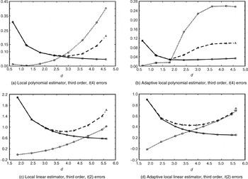
Some selected representative results are reported in graphics. Figure 1(a–d) depicts the biases (dotted lines), variances (solid lines), and MSEs (dashed lines) as a function of d (bandwidth). Again, in all these figures, m(x) = x4. In particular, Figure 1a reports the results of conventional third-order local polynomial estimation for case D3. Figure 1b gives results of the corresponding adaptive (third-order) local polynomial estimator with the same data. Figures 1c and 1d report local linear estimation results corresponding to case D2; in particular, Figure 1c is the conventional local linear estimator, and Figure 1d corresponds to the adaptive local linear estimator. A comparison between biases and standard errors indicates that the variance effect is relatively large over a range of bandwidth choices and thus a relatively large bandwidth is needed to minimize the MSEs.

Representative results (····· = biases, ——— = variances, and ---- = MSEs).
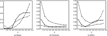
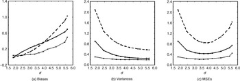
Figures 2 and 3 provide a comparison of the local polynomial estimator (dashed lines), the infeasible local likelihood estimator (dotted lines), and the adaptive estimator (solid lines) in terms of biases, variances, and MSEs. In particular, Figure 2(a–c) compares the conventional third-order local polynomial estimator and the corresponding adaptive estimator for case D3 in biases (Figure 2a), variances (Figure 2b), and MSEs (Figure 2c). Figure 3(a–c) compares the conventional local linear estimator and the adaptive estimator for case D2 in biases (Figure 2a), variances (Figure 2b), and MSEs (Figure 2c). Other cases are qualitatively similar.

Comparison of the conventional third-order local polynomial estimator and the corresponding adaptive estimator for case D3. (---- = the local polynomial estimator, ···· = the infeasible local likelihood estimator, and ——— = the adaptive local polynomial estimator.)

Comparison of the conventional local linear estimator and the adaptive estimator for case D2. (---- = the local polynomial estimator, ···· = the infeasible local likelihood estimator, and ——— = the adaptive local polynomial estimator.)
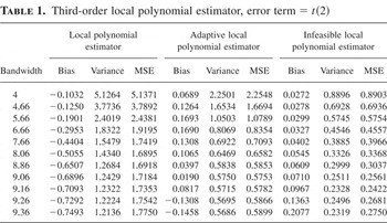
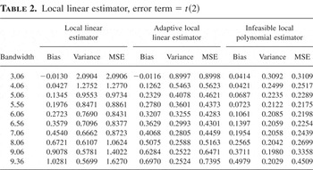
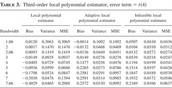
For a more detailed comparison, see Tables 1, 2, and 3. Tables 1 and 3 report the third-order local polynomial estimation results for designs D1 and D2. Table 2 reports the local linear estimation results for D2. Because the student-t distribution has a heavy tail and is different from normal, efficiency gain can be observed from the adaptive procedure. Although the nonparametric estimation introduces additional estimation error significantly, which is reflected from a comparison between the adaptive estimator and the infeasible local likelihood estimator, it is still clear that the adaptive estimators generally have smaller variances than the conventional estimator. They also have smaller MSE in most cases.
Third-order local polynomial estimator, error term = t(2)

Local linear estimator, error term = t(2)

Third-order local polynomial estimator, error term = t(4)

Another specification for the regression function, m(x) = x2, is also considered in the experiment. The Monte Carlo results are similar (and thus not reported in this version) except that we got a smaller bias term in this case. Note that β(x) = M−1Bm(p+1)(x) and when m(x) = x2, m(j)(x) = 0 for all j ≥ 3. Thus we expect the estimation bias to be much smaller than the standard errors, and a large bandwidth is needed to minimize the MSEs because the variance is the main contribution to the MSE.
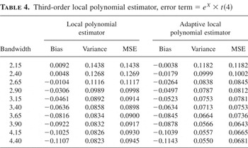
In the case with multiplicative heteroskedasticity, we investigated designs D3 and D4. We first considered case D4. We examined the sampling performance of the third-order (p = 3) local polynomial estimation using the same kernel functions as before and compared the conventional local polynomial estimator with the adaptive local polynomial estimator. Table 4 reports the biases, variances, and MSEs of these estimators using different bandwidth choices. In our experiment, although the error terms ui are not independent of the regressors, the adaptive estimator still has reasonably good sampling performance and improves upon the conventional estimator. One reason for this observation is probably the fact that εi is symmetrically distributed, and our estimator may still preserve adaptiveness, thus leading to better performance than the conventional estimator. To consider this, we then conducted a Monte Carlo experiment using a different (asymmetric) distribution of εi. In the last design (D4), we consider

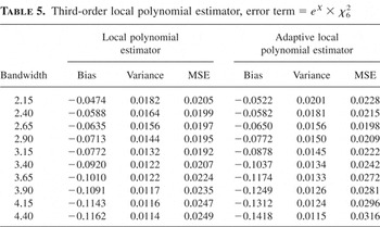
where χ62 are i.i.d. random variables of chi-square distribution with 6 degrees of freedom and re-centered around zero. Results of biases, variances, and MSEs of the two estimators using different bandwidth choices are reported in Table 5. From Table 5, we can see that the estimation bias is relatively much larger than in the previous cases, for both estimators. However, the conventional local polynomial estimation displays better performance in this case.
Third-order local polynomial estimator, error term = eX × t(4)

Third-order local polynomial estimator, error term = eX × χ62

In summary, our simulations indicate that the proposed estimator does a reasonable job for nonparametric estimation.
6. CONCLUSIONS AND EXTENSIONS
We have shown that our estimator of the regression function is adaptive and improves upon the standard local polynomial estimators in terms of asymptotic variance. We have nowhere assumed symmetry. However, we have assumed throughout some fairly minimal moment conditions typically assumed in analysis of regression estimators. These moment conditions are essential to the interpretation of our results but are fairly weak in practice as most economic and financial data sets would have tail thickness in excess of three. One can also obtain results under weaker moment conditions, but then one has (a) to change the interpretation of the estimand or rather make some other identifying assumption such as symmetric errors; (b) to benchmark against more computationally demanding nonlinear estimators such as local median regression.
We have obtained results about the pointwise properties of the estimator of m and its derivatives. One may also be interested in estimating other functionals such as the average derivative of m and the conditional cumulative distribution function (c.d.f.) FY |X. In both these cases, one can obtain expect efficiency improvements under our conditions by using our efficient estimator of m and f in place of the standard procedures. See for example Akritas and Van Keilegom (2001).
APPENDIX
We provide a sketch of the proof of Theorem 1 in this Appendix. A longer version of the proof with details is available from the authors upon request. We denote φ(x,y,z,…) as a general function whose exact form may change from case to case. For simplicity, we denote

and Gb(fi) as

and Gi. For two random variables Xn,Yn, we say that Xn ≃ Yn whenever Xn = Yn(1 + op(1)) as n → ∞. Let Ei denote expectation conditional on the sigma field generated by zi = (Xi,Yi). In what follows we drop the argument x of θ(x),θ0(x),

, and

.
A.1. Preliminaries.
Minimizing (2) with respect to θk gives an estimate

and

, where e1 = (1,0,…,0)[top ] is the vector with the one in the first position, Mn(x) and Ψn(x) are symmetric

matrix and N × 1–dimensional column vector, respectively, and are defined as

where Mn,| j|,|k|(x) is an N| j| × N|k|–dimensional submatrix with the (l,r) element given by

and Ψn,| j|(x) is an N| j|-dimensional subvector whose rth element is given by

The estimate of m(x) is given by

, and its bias and variance effects can be written as

. The stochastic term Un(x) and the bias term Bn(x) are N × 1 vectors

where Un,l(x) and Bn,l(x) are defined similarly as Ψn,l(x) so that Un,| j|(x) and Bn,| j|(x) are N| j|-dimensional subvectors whose rth elements are given by

where Δi(x) = m(Xi) − (1/k!)[sum ]0≤|k|≤p(Dkm)(x)(Xi − x)k.
Under Assumptions A1–A6, we have the following results:

which follow from the results of Masry (1996a). For notational convenience, now define

, where

and define

, where

. Thus

can be written as

. To facilitate asymptotic analysis, we also define the kernel density and derivative estimator based on the unobserved errors

LEMMA A. Under our conditions


Remark A1. The uniform rate given by (A.3) is not the best result, but it suffices for our purpose of proofs in this paper. In fact, following a similar analysis as Masry (1996a), a better rate—Op(hq + n−1/2h−d/2 log(n))—could be obtained with substantially more complicated analysis.
Remark A2. The preceding results can be extended to estimates of derivatives based on similar analysis. The preceding results also hold for any

in a small neighborhood of εi, say,

.
A.2. Proof of Theorem 1.
For notational simplicity, we write

as

and

as

. The estimator

can be written, after standardization by

, as

Let

We expand

around the true value of θ and obtain

where θ* is an intermediate value between θ and

. Based on (A.5), we obtain the complete expansion of

. The preliminary estimator

is consistent and indeed satisfies

. Under the given assumptions, we have

where

Notice that

and substituting (A.6) into (A.4) we may express

as

because

is an

-consistent estimator of θ(x) under our assumptions. Furthermore, it can be shown that

and

. Therefore,

and in fact

Finally, we show that

In the following three sections, we derive the asymptotic results for the Hessian

, the score

, and the remainder term R(θ0).
A.2.1. The Hessian.
We want to show that

We write

and

as

and

, respectively. Thus

We decompose

as

and decompose

as

. By a geometric expansion,

can be written as

Thus we have the following decomposition of

:

where

We show that

and

. This is carried out in a series of lemmas given subsequently.
LEMMA H1. Under our conditions,

.
Proof.

contains the errors coming from the local deviation from Xi to x in terms of δi = εi − εi, which is largely determined by the smoothness property of m(·). For simplicity of exposition, we denote f′/f as ψ. Thus,

Because {εi} and {Xi} are i.i.d. and are mutually independent, for each d-tuple j with 0 ≤ | j| ≤ 2p

by a change of variables and dominated convergence. By a law of large numbers for independent random variables we have

Now we examine

. Define ρ(δ) = ∫[ψ(ε + δ)2 − ψ(ε)2] f (ε) dε for any δ. This quantity is finite, is differentiable, and satisfies ρ(0) = 0. By independence of εi and Xi we have

By dominated convergence, each element in this expectation is zero because as h → 0, maxi:|Xi−x|≤h|m(Xi) − m(x)| = maxi:|Xi−x|≤h|δi| → 0 by the differentiability of m at x. █
LEMMA H2. Under our conditions,

.
Proof. Under our conditions

. In particular, notice that under our bandwidth assumption,

and thus

. Let Gi = Gb(fi). Then,

Therefore, we can ignore the estimation errors in trimming effect. Furthermore, making an expansion of ψ(εi) we obtain

We verify the orders of magnitude for these terms. It can be shown that the leading trimming term is determined by

with elements

Notice that

Under Assumption A1 (or A1′ and A1′′), we can show that

The precise order of magnitude of the trimming effect will depend on the tail behavior of f. In addition, E [K((x − Xi)/h)((x − Xi)/h)j] = hdfX(x)μj(K). By i.i.d. assumption, we have

Other terms can be analyzed similarly. █
For j = 3,4,…,10, terms

are functions of

and/or

. To facilitate asymptotic analysis, we decompose

into the sum of

and f′(εi) − f′(εi) (and

into the sum of

and f (εi) − f (εi)). The first term,

, contains errors coming from preliminary estimation

and

, and the second term, f′(εi) − f′(εi), contains the errors coming from nonparametric kernel smoothing.
LEMMA H3. Under our conditions,

.
Proof. We decompose

and obtain

Because |ν(x)| = Op(hp+1 + n−1/2h−d/2), to show that

, we show that, for each d-tuple τ with 0 ≤ |τ| ≤ 2p,

Let

For the preceding result it can be verified that the first two moments of

are

. For

, because

, we expand Mn−1(Xj) around its limit (Mf (Xj))−1 and get Mn−1(Xj) = (Mf (Xj))−1 − (Mf (Xj))−1 × [Mn(Xj) − MfX(Xj)]Mn−1(Xj). Then we show that each of the terms in the expansion is op(1). To show

, we decompose f′(εi) − f′(εi) into a bias effect B′(εi) and a variance effect V′(εi) and, again, analyze second-order U-statistics with degeneracy. Similar analysis can be applied to other terms that involve

and

.
The analysis for

,

,

, and

is similar. The terms

,

, and

contain

in the denominator. Under our assumptions, for each d-tuple τ with 0 ≤ |τ| ≤ 2p,

Thus

. We have used Lemma A here. Similar analysis can be conducted for

and

. █
A.2.2. The score function.
We want to show that

By definition

For the denominator,

, where

. Therefore,

We analyze the asymptotic behavior of Tj, j = 1,2,…,5.
LEMMA S1. Under our conditions

where

.
Proof. Notice that

and

We verify each of these terms. First, by a central limit theorem for i.i.d. random vectors,

For the second term,

For each d-tuple τ with 0 ≤ |τ| ≤ 2p,

Therefore,

Similarly, by calculation of moments, it is easy to verify that under our conditions,

and T14 are

. █
LEMMA S2. Under our conditions,

.
Proof. First, we expand the trimming function to the second order,

where fi* is an intermediate point between

and fi. Then

We use a crude bound on the last term and show that it is op(1). Therefore, we must analyze the term

This again involves some further U-statistic calculation. Similar to the previous analysis, we decompose (A.10) into T21 + T22, where

Further,

For the leading term T21A, because ν(x) = Op(hq + n−1/2h−d/2), we need to show that for each 0 ≤ |τ| ≤ 2p,

Notice that

We need to show that

Conditional on Xi,

Notice that g(·) ≥ 0 is bounded, say, g(·) ≤ C; then

Thus

By Assumption A3, we have

by dominated convergence, because ∫b≤f (v)≤2b(f′(v)2/f (v)) dv ≤ I(f) < ∞. Therefore,

Consequently, under our bandwidth conditions,

Thus T21A = op(1). For T21B, following similar analyses as those in the proof of Lemma H3, we can verify that each of these terms is op(1).
The second component of errors comes from standard kernel estimation and can be analyzed similarly. We decompose f (εi) − f (εi) into a bias effect

and a variance effect

. Thus

The variance term is

Denote, for each 0 ≤ |τ| ≤ 2p,

Again, this is a second-order U-statistic with degeneracy and

We show T22A = op(1) by verifying the orders of magnitude of E [γ3n(zi,zj)2], E [γ3n(zi,zj)γ3n(zj,zi)], and E [γ3n(zi,zj)γ3n(zl,zj)].
The leading bias term is

Thus T22 = op(1). Consequently the term (A.10) = op(1).
Finally we turn to the leading term of T2,

Again, we denote f′/f as ψ and under given assumptions we obtain a Taylor expansion that ψ(εi) ≃ ψ(εi) + ψ′(εi)δi. Thus, the preceding term can be approximated by


To verify the order of magnitude of (A.11), we calculate the first two moments. Notice that under our assumptions, ψ(εi)[1 − Gi] are i.i.d. and

For b small enough, there exists −∞ < a1 < a2 < a2 < a1 < ∞ such that

where f (a1) = f (a1) = b and f (a2) = f (a2) = 2b. Therefore,

Notice that

and

. Thus ψ(εi)[1 − Gi] are mean zero. Thus we just need to verify the second moment of (A.11). Notice that


under Assumption A1 (or A1′ and A1′′). Thus, combining (A.13) and (A.14), we can show that the order of (A.11) is op(1). If we assume that Assumption A1′′ holds, it can be shown that

and the order of magnitude of (A.11) is Op(b(s−1)/(2s)) = op(1).
Now we look at the term (A.12). Notice that E [K((x − Xi)/h)δi] ≃ hd+qφ(K,m,fX), where φ(K,m,fX) is a function of the kernel and derivatives of m and fX evaluated at x. And E [ψ′(εi)(1 − Gi)] = o(1). Consequently, by calculation of moments we have, under bandwidth assumption A7, (A.12) = op(1). █
LEMMA S3. Under our conditions

Proof. The analysis of T3 is similar to that of

.

and

Analysis of these terms will then be similar to the previous analysis. In particular, we can show that the variance term is op(1) and, for the bias term, for each d-tuple τ with 0 ≤ |τ| ≤ 2p,

Thus

For T32A, it is again a second-order U-statistic with first-order degeneracy and can be analyzed in a similar way to the proof of T22A.
For T32B, notice that, conditional on X1,…, Xn,

It is easy to show that

█
LEMMA S4. Under our conditions

Proof. The proof is similar to that of Lemma S3. █
LEMMA S5. Under our conditions,

.
Proof. For the remainder terms T5, we need to show that

goes to zero as n → ∞. Notice that for each 0 ≤ |τ| ≤ 2p,

Because

, and using the result (A.3), the remainder term is of order Op(n1/2hd/2)Op(b−2)Op(h02q−2 + n−1h0−d−2 log2(n)), which is op(1) under our bandwidth conditions. █
A.2.3. Remainder term.
It suffices to show that

and

because

. The expression for Rn(θ*) is quite complicated, but its analysis is similar to that of the Hessian except that (a) we require only bounds in probability that are quite weak; (b) those bounds, however, have to be locally uniform in the argument θ. By an analysis similar to that of the Hessian, it can be shown that

for any given θ. The extension to local uniform over {θ : ∥θ − θ0∥ ≤ n−1/2h−d/2} follows from the smoothness properties on the kernel that we have imposed. We just examine a single key term

By construction

, whereas

. Therefore, |Rn1*(θ)| = Op(h0−4b−1). Therefore, (A.16) is satisfied because

is assumed to go to zero under our condition. By expanding out we can obtain better results but with considerably more calculations.
For R(θ0), by an analysis similar to that of the score and also using the result of Lemma A, we can show that it is op(1). █