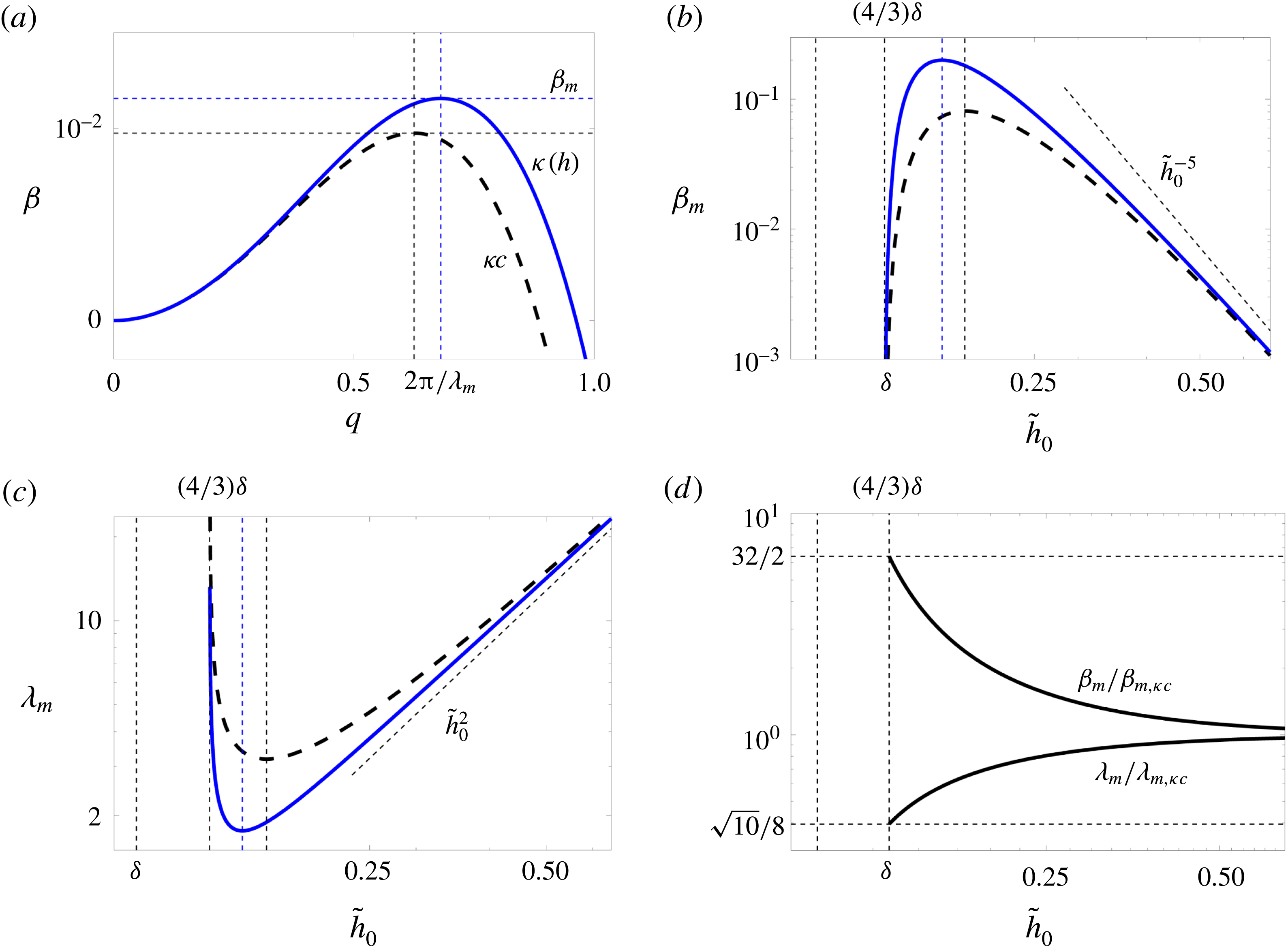
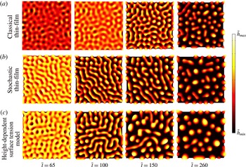
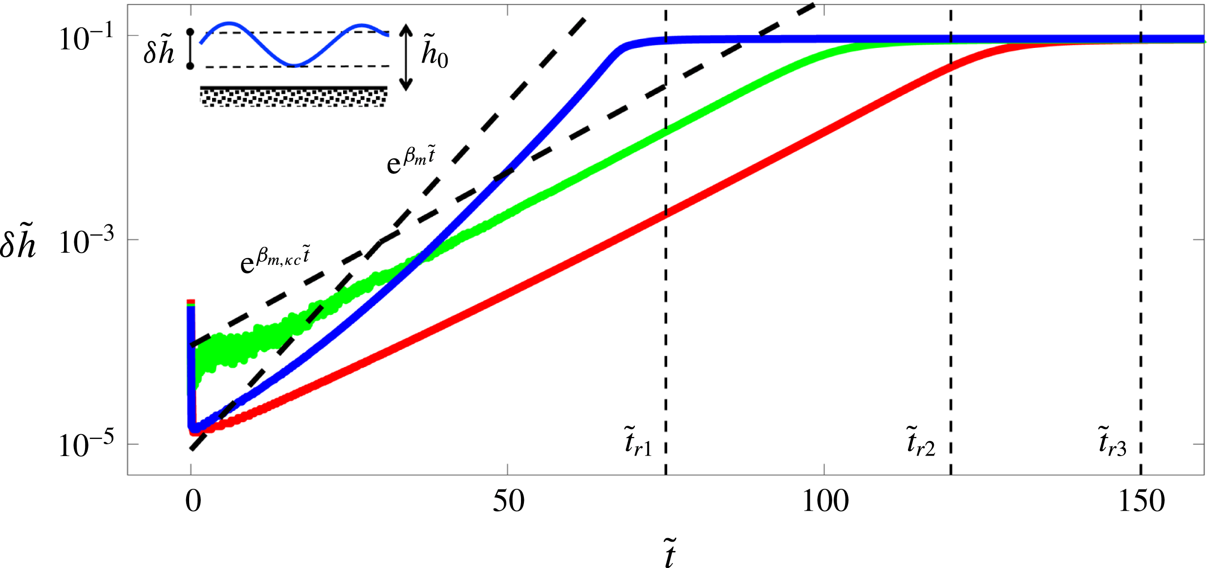
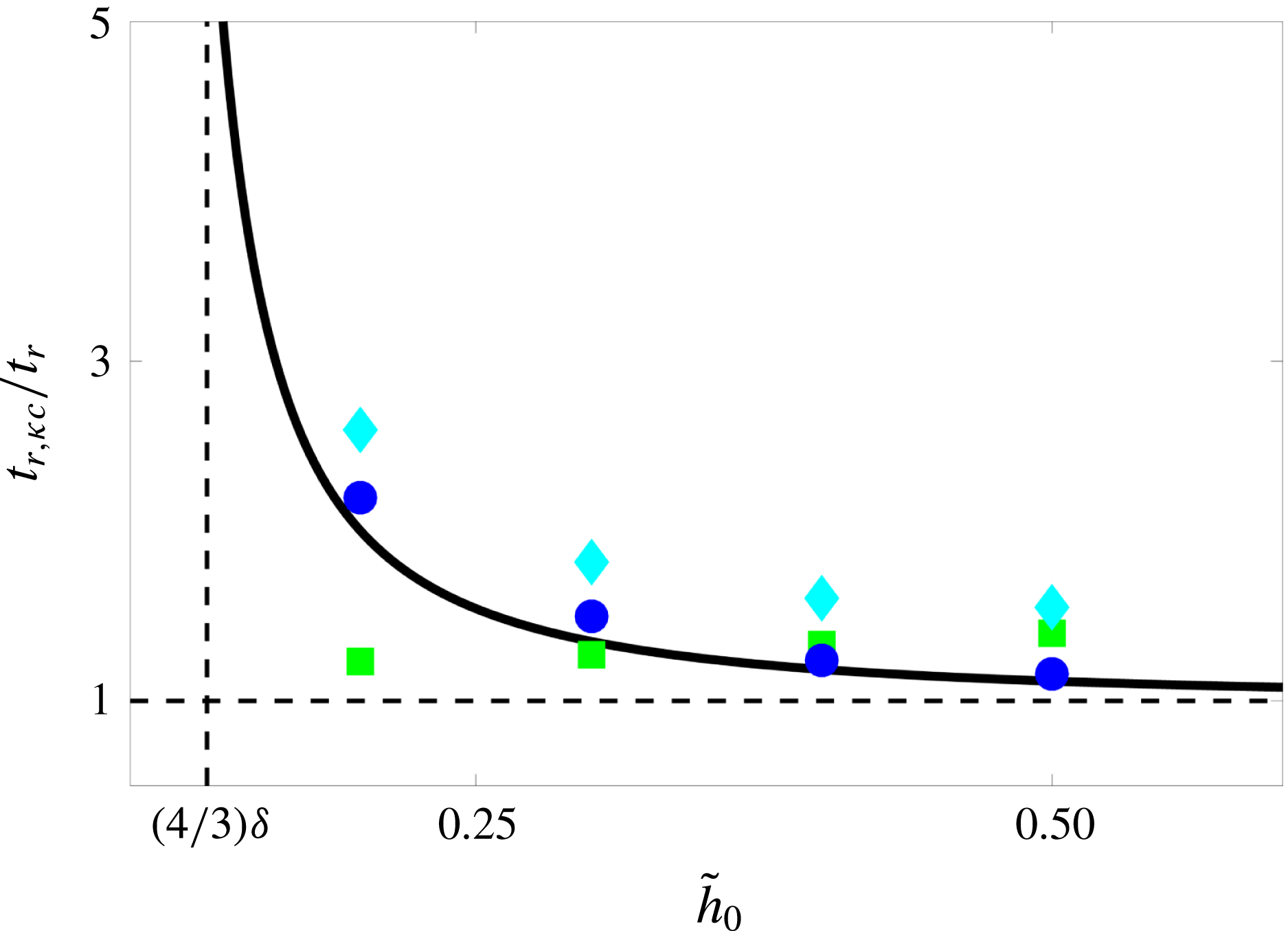
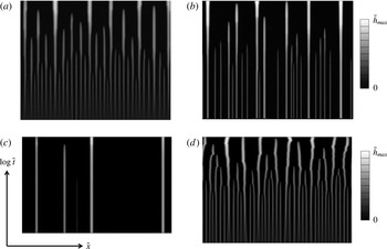
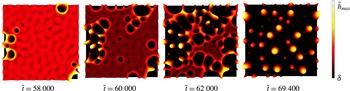
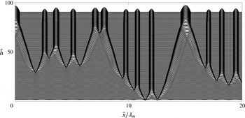
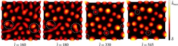
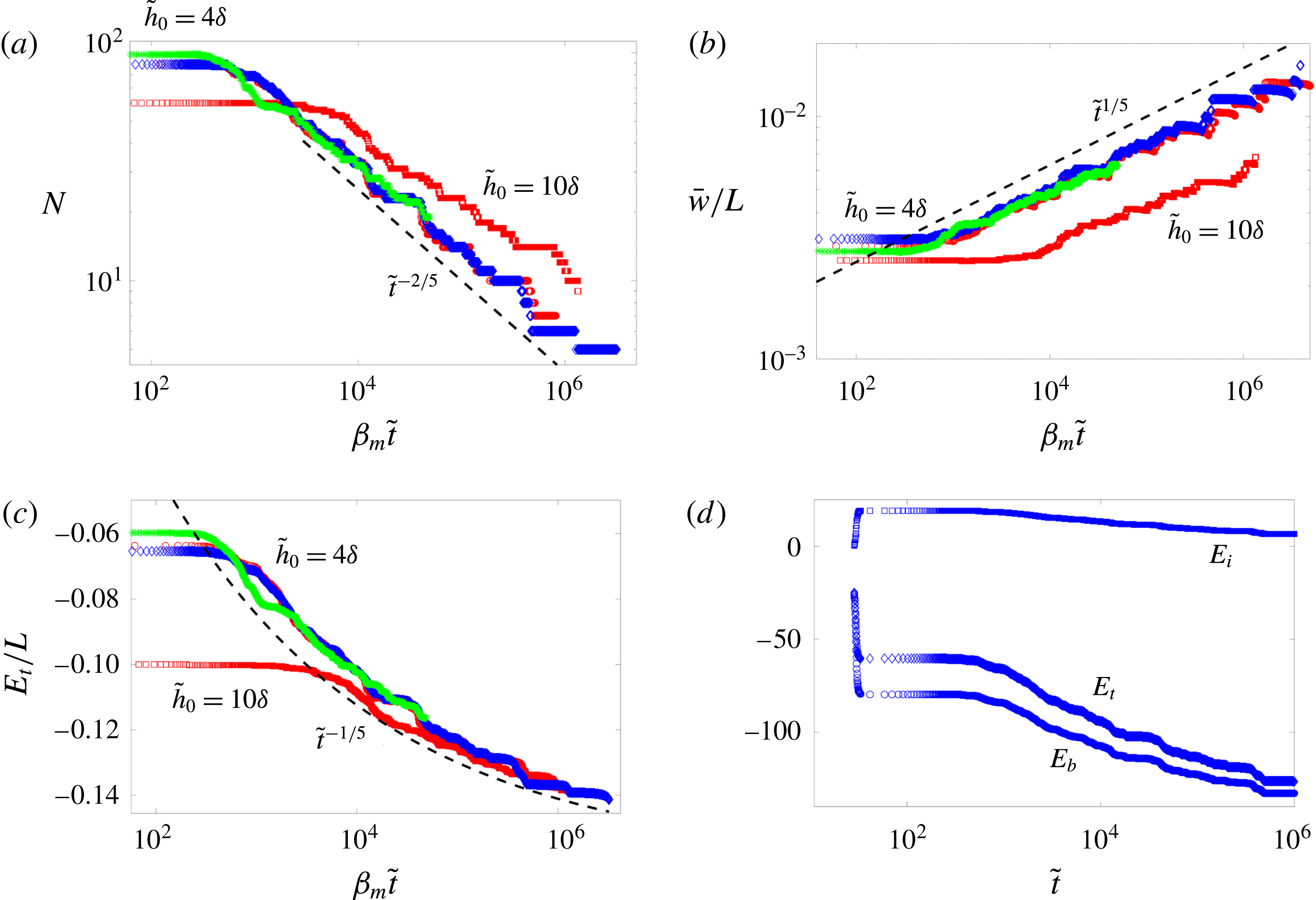
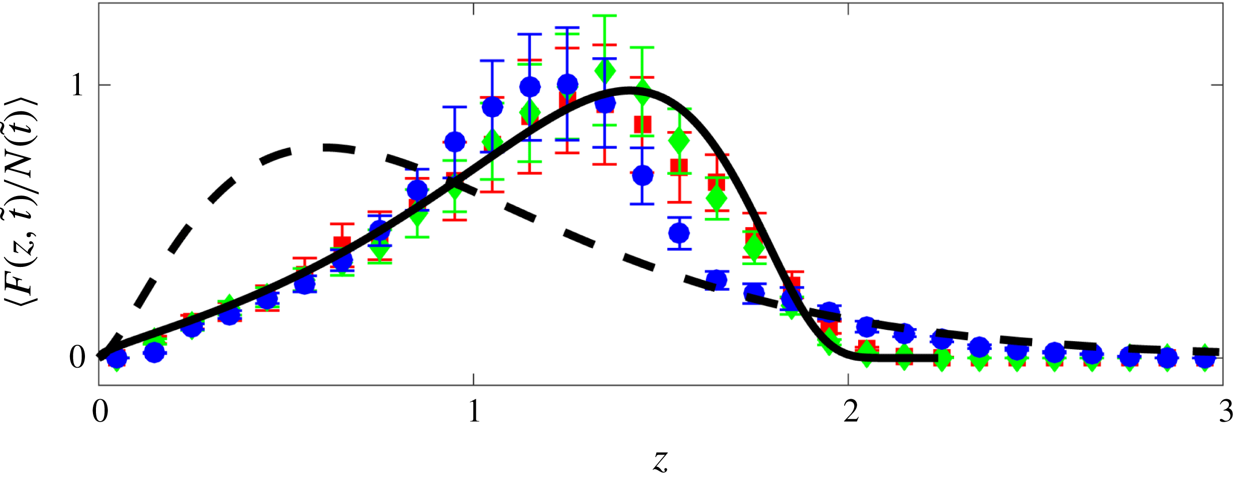
1 Introduction
Understanding the underlying physics of how fluids coat solid substrates has been a long-standing quest in fluid dynamics (Blake & Ruschak Reference Blake and Ruschak1979; Ruschak Reference Ruschak1985; Quéré Reference Quéré1999; Weinstein & Ruschak Reference Weinstein and Ruschak2004; Snoeijer & Andreotti Reference Snoeijer and Andreotti2013). With the advent of micro and nanoscale lithography techniques enabling manipulation at increasingly small scales (Xia & Whitesides Reference Xia and Whitesides1998; Gates et al.
Reference Gates, Xu, Stewart, Ryan, Willson and Whitesides2005; Qin, Xia & Whitesides Reference Qin, Xia and Whitesides2010), and with applications ranging from micro/nanofluidics to additive manufacturing (Stone, Stroock, & Ajdari Reference Stone, Stroock and Ajdari2004; Schoch, Han & Renaud Reference Schoch, Han and Renaud2008; Wijshoff Reference Wijshoff2010; Kumar Reference Kumar2015), questions arise regarding the relevant description of fluid physics at the nanoscale and the validity of continuum modelling at such small scales (Squires & Quake Reference Squires and Quake2005; Bocquet & Charlaix Reference Bocquet and Charlaix2010; Colin, Squires & Bocquet Reference Colin, Squires and Bocquet2012; Bocquet & Tabeling Reference Bocquet and Tabeling2014; Lohse & Zhang Reference Lohse and Zhang2015). As the thickness of a liquid film on a solid substrate becomes smaller than approximately
 $100~\text{nm}$
, the atoms at the liquid–solid and liquid–gas interfaces start interacting with each other, giving rise to additional intermolecular forces that need to be considered in continuum modelling (Rauscher & Dietrich Reference Rauscher and Dietrich2008; Bonn et al.
Reference Bonn, Eggers, Indekeu, Meunier and Rolley2009; Israelachvili Reference Israelachvili2011).
A uniform nanometric thin liquid film on a solid substrate can become unstable due to these intermolecular forces. The instability leads to dewetting of the film and the formation of drops. Both liquid and solid-state dewetting at the nanoscale are relevant in many phenomena (Blossey Reference Blossey2012; Gentili et al. Reference Gentili, Foschi, Valle, Cavallini and Biscarini2012; Thompson Reference Thompson2012; Mukherjee & Sharma Reference Mukherjee and Sharma2015; Pierre-Louis Reference Pierre-Louis2016) such as pumping liquids using nanowires (Huang et al. Reference Huang, Lo, Niu, Kushima, Qian, Zhong, Mao and Li2013), patterning via self-assembly (Gau et al. Reference Gau, Herminghaus, Lenz and Lipowsky1999; Higgins & Jones Reference Higgins and Jones2000; Lopes & Jaeger Reference Lopes and Jaeger2001; Huang et al. Reference Huang, Kim, Tao, Connor and Yang2005; Segalman Reference Segalman2005; van Hameren et al. Reference van Hameren, Schön, van Buul, Hoogboom, Lazarenko, Gerritsen, Engelkamp, Christianen, Heus, Maan, Rasing, Speller, Rowan, Elemans and Nolte2006; Pokroy et al. Reference Pokroy, Kang, Mahadevan and Aizenberg2009; Fowlkes et al. Reference Fowlkes, Kondic, Diez, Wu and Rack2011; Han & Lin Reference Han and Lin2012; Thiele Reference Thiele2014; Kong et al. Reference Kong, Boulogne, Kim, Nunes, Feng and Stone2015, Reference Kong, Gupta, Johnson and McAlpine2016; Wu et al. Reference Wu, Dong, Kuang, Li, Li, Jiang and Song2015), synthesis of core–shell nanoparticle arrays (McKeown et al. Reference McKeown, Wu, Fowlkes, Rack and Campbell2015), droplet generation (Yamamoto et al. Reference Yamamoto, Nakajima, Shioi, Krafft and Yoshikawa2015; Keiser et al. Reference Keiser, Bense, Colinet, Bico and Reyssat2017), needle growth (Yu, Bulović & Hosoi Reference Yu, Bulović and Hosoi2013), understanding slip and rheology of nanometric films (Herminghaus, Seemann & Jacobs Reference Herminghaus, Seemann and Jacobs2002; Fetzer et al. Reference Fetzer, Jacobs, Münch, Wagner and Witelski2005, Reference Fetzer, Münch, Wagner, Rauscher and Jacobs2007a ; Bäumchen & Jacobs Reference Bäumchen and Jacobs2010; Bäumchen et al. Reference Bäumchen, Fetzer, Klos, Lessel, Marquant, Hähl and Jacobs2012; Bäumchen et al. Reference Bäumchen, Marquant, Blossey, Münch, Wagner and Jacobs2014; McGraw et al. Reference McGraw, Bäumchen, Klos, Haefner, Lessel, Backes and Jacobs2014), tear film dynamics (Braun Reference Braun2012), film flow in heat pipes (Kundan et al. Reference Kundan, Nguyen, Plawsky, Wayner, Chao and Sicker2017), Rayleigh–Plateau instability of nanowires or liquids in nanochannels (Molares et al. Reference Molares, Balogh, Cornelius, Neumann and Trautmann2004; Chen, Zhang & Russell Reference Chen, Zhang and Russell2007), or stability of bubbles/drops in micro/nanochannels (Huerre et al. Reference Huerre, Theodoly, Leshansky, Valignat, Cantat and Jullien2015; Hammoud et al. Reference Hammoud, Trinh, Howell and Stone2017).
Reiter (Reference Reiter1992, Reference Reiter1993) was the first to experimentally characterize the dewetting of a nanometric polymer film on a solid substrate. He observed that, initially, some holes form with a seemingly characteristic wavelength between them; these holes then expand with a ridge formed at the receding front; these ridges ultimately meet and form a network of polygonal patterns. The ridges later collapse due to the Rayleigh–Plateau instability, forming small droplets of approximately uniform size. On a much longer time scale still, these droplets can coarsen to ultimately form a single drop; the time scale associated with this last stage, however, is very long and not readily accessible within typical experiments.
The theory for instability of thin liquid films under the influence of intermolecular forces far predates the experimental observations, dating back to Vrij (Reference Vrij1966), Sheludko (Reference Sheludko1967), Ruckenstein & Jain (Reference Ruckenstein and Jain1974), Williams & Davis (Reference Williams and Davis1982), Wyart & Daillant (Reference Wyart and Daillant1990), Brochard-Wyart, Martin & Redon (Reference Brochard-Wyart, Martin and Redon1993), Sharma & Reiter (Reference Sharma and Reiter1996), Sharma & Khanna (Reference Sharma and Khanna1998) and Oron (Reference Oron2000). The Navier–Stokes equations describing the fluid motion can be greatly simplified using the long-wave/lubrication approximation when the characteristic lateral length of the flow is much larger than its characteristic height, an approach that has its origins in the work of Reynolds to describe the pressure distribution for slider bearings (Reynolds Reference Reynolds1886). For ultrathin liquid films, an additional disjoining pressure term arises due to the intermolecular interactions between the solid–liquid and liquid–gas interfaces.
Assuming a particular form for the intermolecular forces, one can use linear stability analysis of the thin-film equation to arrive at a prediction for the scaling of the wavelength of the instability and its growth rate as a function of the initial uniform film thickness (Oron, Davis & Bankoff Reference Oron, Davis and Bankoff1997; Craster & Matar Reference Craster and Matar2009); this regime predicted by the linear theory is known as the spinodal regime. In apolar systems, typically van der Waals (vdW) forces are the main long-range attractive interactions, scaling with the film thickness as
 ${\sim}1/h^{2}$
, leading to a scaling of
 ${\sim}h^{2}$
and
 ${\sim}1/h^{5}$
for the most unstable wavelength and fastest growth rate, respectively. These scalings therefore serve as a qualitative benchmark for the experiments to determine if they are within the spinodal regime. Making quantitative predictions, however, requires prescribing the exact form of the interface potential.
The observations by Reiter (Reference Reiter1992, Reference Reiter1993) led to a wave of experimental studies focusing on dewetting of thin liquid films. Jacobs, Herminghaus & Mecke (Reference Jacobs, Herminghaus and Mecke1998) showed that the holes observed in the experiments of Reiter (Reference Reiter1992, Reference Reiter1993) have a Poisson distribution, a signature of the nucleation regime, and that the scaling of the film-rupture time as a function of film thickness did not match the theoretical predictions of the spinodal regime; films in the nucleation regime are linearly stable, yet instabilities can still grow due to the presence of defects on the substrate or in the film itself (Jacobs et al. Reference Jacobs, Herminghaus and Mecke1998). The first observations of the spinodal regime were reported by Bischof et al. (Reference Bischof, Scherer, Herminghaus and Leiderer1996) and Herminghaus et al. (Reference Herminghaus, Jacobs, Mecke, Bischof, Fery, Ibn-Elhaj and Schlagowski1998) using thin gold films on quartz substrates, where the correlations between the holes was rigorously shown using Minkowski functionals (Mecke Reference Mecke1998; Mantz, Jacobs & Mecke Reference Mantz, Jacobs and Mecke2008).
The presence of residual stresses in thin polymer films can further complicate the dewetting process; Reiter et al. (Reference Reiter, Hamieh, Damman, Sclavons, Gabriele, Vilmin and Raphael2005) observed dewetting through nucleation for large film thicknesses, where the film is expected to be linearly stable. They realized that the number of holes is a strong function of the ageing time of the polymer before the temperature is raised above the glass transition temperature to perform the experiments; they further speculated that the reason behind this observation could be that during the spin-coating process, the solvent evaporates quickly, leaving the polymer chains in non-equilibrium configurations leading to a residual stress in the film, which can be responsible for the unexpected instability of the films. The observations by Reiter et al. (Reference Reiter, Hamieh, Damman, Sclavons, Gabriele, Vilmin and Raphael2005) therefore point to the need for extreme caution in conducting and interpreting experiments on thin films in spinodal and nucleation regimes (Stange, Evans & Hendrickson Reference Stange, Evans and Hendrickson1997; Thiele, Mertig & Pompe Reference Thiele, Mertig and Pompe1998; Xie et al. Reference Xie, Karim, Douglas, Han and Weiss1998; Segalman & Green Reference Segalman and Green1999; Meredith et al. Reference Meredith, Smith, Karim and Amis2000; Bollinne et al. Reference Bollinne, Cuenot, Nysten and Jonas2003; Sharma Reference Sharma2003; Nguyen et al. Reference Nguyen, Fuentes-Cabrera, Fowlkes and Rack2014).
Seemann, Herminghaus & Jacobs (Reference Seemann, Herminghaus and Jacobs2001a ) conducted a series of well-controlled experiments using polystyrene films spin-cast on silicon (Si) wafers. They demonstrated that by tuning the thickness of the silicon oxide coating of the Si wafer, they could alter the interface potential and classify three categories of instabilities: (1) spinodal dewetting for linearly unstable regions, (2) thermal nucleation at the edge of the linearly unstable region, where thermal fluctuations can overcome the energy barrier leading to dewetting, and (3) heterogeneous nucleation within the linearly stable region, where defects on the substrate or in the film give rise to the appearance of holes and instabilities. The spinodal regime is easily distinguishable as it gives rise to a well-defined characteristic wavelength of instability, from which the interface potential can be reconstructed. The key feature distinguishing regimes 2 and 3 is that holes continuously appear throughout the experiment in the thermal nucleation regime, whereas they all form within a limited time window in the heterogeneous nucleation regime.
Becker et al. (Reference Becker, Grun, Seemann, Mantz, Jacobs, Mecke and Blossey2003) observed good agreement between experimental observations and theoretical predictions, with the caveat that experiments showed a faster rupture time. To explain the time-scale mismatch between theory and experiments, Mecke & Rauscher (Reference Mecke and Rauscher2005), Grün, Mecke & Rauscher (Reference Grün, Mecke and Rauscher2006) and Fetzer et al. (Reference Fetzer, Rauscher, Seemann, Jacobs and Mecke2007b ) suggested that accounting for thermal fluctuations is necessary. They showed that thermal noise at the typical temperatures used in the experiments can speed up the initial rupture process, thereby bringing the theoretical predictions closer to the experimental observations.
Here, we revisit the theory of thin liquid films in partial wetting and show that the intermolecular forces in thin films give rise to a height-dependent surface tension. We show that the free energy of the system can be cast in the following form:
 $$\begin{eqnarray}\displaystyle & \displaystyle \unicode[STIX]{x1D6E4}=\int \left(f(h)+{\displaystyle \frac{1}{2}}\unicode[STIX]{x1D705}(h)(h_{x})^{2}\right)\text{d}x, & \displaystyle\end{eqnarray}$$
which resembles the Cahn–Hilliard framework for phase separation in binary alloys (Cahn & Hilliard Reference Cahn and Hilliard1958; Langer Reference Langer1971), an idea that dates back to van der Waals (Rowlinson Reference Rowlinson1979; Rowlinson & Widom Reference Rowlinson and Widom2013). Here,
 $f(h)$
is the bulk free energy and
 $\unicode[STIX]{x1D705}(h)$
is a height-dependent surface tension term; this feature has important consequences for stability of liquid films, leading to a slightly smaller wavelength of instability and a faster rupture rate than the classical theory (by up to six times), bringing the theory closer to the experimental observations, and suggesting that the height dependence of surface tension could play a role along with the presence of thermal noise.
Within the framework of non-equilibrium thermodynamics (Hohenberg & Halperin Reference Hohenberg and Halperin1977; Cross & Hohenberg Reference Cross and Hohenberg1993; Bray Reference Bray2002), our model in non-dimensional form can be written succinctly as follows (Pahlavan et al. Reference Pahlavan, Cueto-Felgueroso, McKinley and Juanes2015):
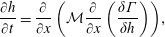 $$\begin{eqnarray}\displaystyle & \displaystyle {\displaystyle \frac{\unicode[STIX]{x2202}h}{\unicode[STIX]{x2202}t}}={\displaystyle \frac{\unicode[STIX]{x2202}}{\unicode[STIX]{x2202}x}}\left({\mathcal{M}}{\displaystyle \frac{\unicode[STIX]{x2202}}{\unicode[STIX]{x2202}x}}\left({\displaystyle \frac{\unicode[STIX]{x1D6FF}\unicode[STIX]{x1D6E4}}{\unicode[STIX]{x1D6FF}h}}\right)\right)\!, & \displaystyle\end{eqnarray}$$
with the mobility
 ${\mathcal{M}}$
, and the pressure defined as the variational derivative of the free energy as
 $\tilde{P}=\unicode[STIX]{x1D6FF}\unicode[STIX]{x1D6E4}/\unicode[STIX]{x1D6FF}h=\text{d}f/\text{d}h-\sqrt{\unicode[STIX]{x1D705}}\unicode[STIX]{x2202}/\unicode[STIX]{x2202}x(\sqrt{\unicode[STIX]{x1D705}}\unicode[STIX]{x2202}h/\unicode[STIX]{x2202}x)$
; here,
 $h$
represents the height of the liquid film,
 $\unicode[STIX]{x1D705}$
is the height-dependent surface tension, and
 $f$
is the bulk free energy.
Our model leads to a generalized form of the disjoining pressure defined as:
 $$\begin{eqnarray}\displaystyle & \displaystyle \unicode[STIX]{x1D6F7}(h,h_{x},h_{xx})={\displaystyle \frac{\text{d}\unicode[STIX]{x1D719}_{\unicode[STIX]{x1D707},1}}{\text{d}h}}+\sqrt{\unicode[STIX]{x1D719}_{\unicode[STIX]{x1D707},2}}{\displaystyle \frac{\unicode[STIX]{x2202}}{\unicode[STIX]{x2202}x}}\left(\sqrt{\unicode[STIX]{x1D719}_{\unicode[STIX]{x1D707},2}}{\displaystyle \frac{\unicode[STIX]{x2202}h}{\unicode[STIX]{x2202}x}}\right), & \displaystyle\end{eqnarray}$$
with
 $\unicode[STIX]{x1D719}_{\unicode[STIX]{x1D707},1}(h)$
and
 $\unicode[STIX]{x1D719}_{\unicode[STIX]{x1D707},2}(h)$
as components of the vdW force. As indicated in (1.3), this generalized disjoining pressure depends not only on the film height, but also on its slope and curvature. This model allows describing the spreading and dewetting of drops and thin films in the true partial-wetting regime (Brochard-Wyart et al.
Reference Brochard-Wyart, Di Meglio, Quere and de Gennes1991; de Gennes, Brochard-Wyart & Quéré Reference de Gennes, Brochard-Wyart and Quéré2004) without the need to invoke a precursor film (Pahlavan et al.
Reference Pahlavan, Cueto-Felgueroso, McKinley and Juanes2015).
Using the new thin-film model, we revisit the instability and dewetting of a partially wetting thin liquid film on a solid substrate. We first analyse the equilibrium film and droplet solutions predicted by this model and contrast it with the classical model, showing that in our model the equilibrium droplets exhibit compact support and show a non-zero equilibrium angle at the contact line, whereas the classical thin-film model cannot admit solutions with compact support and the equilibrium droplet only asymptotically meets the substrate through a precursor film (Brenner & Bertozzi Reference Brenner and Bertozzi1993). Analysing the stability of uniform film solutions, we show that the new model predicts a faster growth rate and smaller wavelength of instability in the spinodal regime than the classical model. Upon dewetting, the newly formed liquid droplets arrive at a metastable state; they are connected by ultrathin fluid films of non-zero thickness and slowly coarsen to lower the energy of the system; this coarsening process, however, occurs on very long time scales as the dynamics is now mainly driven by drainage through the ultrathin films and the mobility scales as
 ${\sim}h^{3}$
, leading to very small rates of mass transfer between the droplets. We show that the coarsening process arrives at a self-similar intermediate-asymptotic behaviour (Barenblatt Reference Barenblatt1996), which is independent of the details of the contact-line models and even in the presence of thermal fluctuations matches the existing predictions for the classical thin-film model (Glasner & Witelski Reference Glasner and Witelski2003; Gratton & Witelski Reference Gratton and Witelski2008, Reference Gratton and Witelski2009). We, however, observe a skewed drop-size distribution for larger drops in the new model; while the long-tailed distribution follows a Smoluchowski equation, it is not associated with a coalescence-dominated coarsening process, calling into question the association made between coalescence and skewed drop-size distribution in some earlier experiments.
2 Thin-film model in partial wetting
2.1 Free energy at equilibrium: emergence of Cahn–Hilliard framework with height-dependent surface tension
Consider a nanometric thin liquid film sitting on a solid substrate, as shown in figure 1. When the film is perturbed, it can become unstable if the solid prefers to be in contact with the gas phase; in this configuration the uniform film has the lowest interfacial area, so dewetting lowers the bulk energy of the system at the expense of increasing its interfacial energy. We can write the energy of a half drop in one dimension as
 $$\begin{eqnarray}\displaystyle & \displaystyle \unicode[STIX]{x1D6E4}=\int _{0}^{x_{0}}\unicode[STIX]{x1D719}(h,h_{x})\,\text{d}x, & \displaystyle\end{eqnarray}$$
where
 $\unicode[STIX]{x1D719}$
is the free energy density,
 $x=0$
marks the centre of the drop and
 $x=x_{0}$
is where the liquid, solid and gas meet, i.e. the contact line. At equilibrium, the variation of the free energy is zero, i.e.
 $\unicode[STIX]{x1D6FF}\unicode[STIX]{x1D6E4}=0$
:
 $$\begin{eqnarray}\displaystyle & \displaystyle \unicode[STIX]{x1D6FF}\left(\int _{0}^{x_{0}}(\unicode[STIX]{x1D719}(h,h_{x})-Ph)\,\text{d}x\right)=0, & \displaystyle\end{eqnarray}$$
where the operator
 $\unicode[STIX]{x1D6FF}$
indicates variation of the functional and the Lagrange multiplier
 $P$
is introduced to enforce mass conservation. Expanding the above equation leads to
 $$\begin{eqnarray}\displaystyle & \displaystyle \int _{0}^{x_{0}}\left({\displaystyle \frac{\unicode[STIX]{x2202}\unicode[STIX]{x1D719}}{\unicode[STIX]{x2202}h}}-P\right)\unicode[STIX]{x1D6FF}h\,\text{d}x+\int _{0}^{x_{0}}{\displaystyle \frac{\unicode[STIX]{x2202}\unicode[STIX]{x1D719}}{\unicode[STIX]{x2202}h_{x}}}\unicode[STIX]{x1D6FF}h_{x}\,\text{d}x+\unicode[STIX]{x1D719}|_{x_{0}}\unicode[STIX]{x1D6FF}x_{0}=0. & \displaystyle\end{eqnarray}$$
Using integration by parts, we can rewrite the second integral in (2.3), leading to
 $$\begin{eqnarray}\displaystyle \displaystyle \unicode[STIX]{x1D6FF}\int _{0}^{x_{0}}(\unicode[STIX]{x1D719}(h,h_{x})-Ph)\,\text{d}x & = & \displaystyle \int _{0}^{x_{0}}\left[{\displaystyle \frac{\unicode[STIX]{x2202}\unicode[STIX]{x1D719}}{\unicode[STIX]{x2202}h}}-{\displaystyle \frac{\text{d}}{\text{d}x}}\left({\displaystyle \frac{\unicode[STIX]{x2202}\unicode[STIX]{x1D719}}{\unicode[STIX]{x2202}h_{x}}}\right)-P\right]\unicode[STIX]{x1D6FF}h\,\text{d}x\nonumber\\ \displaystyle & & \displaystyle \left.+\left({\displaystyle \frac{\unicode[STIX]{x2202}\unicode[STIX]{x1D719}}{\unicode[STIX]{x2202}h_{x}}}\right)\unicode[STIX]{x1D6FF}h\right|_{0}^{x_{0}}+\unicode[STIX]{x1D719}|_{x_{0}}\unicode[STIX]{x1D6FF}x_{0}=0.\end{eqnarray}$$
We can further use the Taylor expansion for the boundary terms and write
 $\unicode[STIX]{x1D6FF}h|_{x_{0}}=-\unicode[STIX]{x1D6FF}x_{0}(\unicode[STIX]{x2202}h/\unicode[STIX]{x2202}x)|_{x_{0}}$
.
Schematic of a liquid film on a solid substrate; films with a height less than approximately
 $100~\text{nm}$
can become unstable to infinitesimal perturbations if the liquid does not completely wet the substrate; in such situations, the instabilities grow and the film dewets from the substrate, forming small droplets that can then coarsen to form larger drops; the shape of the small drops is governed mainly by surface tension, leading to a spherical cap shape with a macroscopic Young contact angle
 $\unicode[STIX]{x1D703}_{Y}$
; deviations from the spherical cap shape can occur due to the intermolecular forces very close to the contact line. If the height of the drop becomes comparable to the capillary length
 $l_{\unicode[STIX]{x1D6FE}}=\sqrt{\unicode[STIX]{x1D6FE}/(\unicode[STIX]{x1D70C}g)}$
, gravitational force becomes important, levelling the drop and forming a puddle shape; gravity sets the upper limit
 $h_{\ast }=2l_{\unicode[STIX]{x1D6FE}}\sin (\unicode[STIX]{x1D703}_{Y}/2)$
for the puddle height.

At equilibrium, the integrand as well as the boundary terms need to be independently zero. The integrand represents the Euler–Lagrange equation (Yeh, Newman & Radke Reference Yeh, Newman and Radke1999; Starov, Velarde & Radke Reference Starov, Velarde and Radke2007; Arfken, Weber & Harris Reference Arfken, Weber and Harris2013)
 $$\begin{eqnarray}\displaystyle & \displaystyle \left[{\displaystyle \frac{\unicode[STIX]{x2202}\unicode[STIX]{x1D719}}{\unicode[STIX]{x2202}h}}-{\displaystyle \frac{\text{d}}{\text{d}x}}\left({\displaystyle \frac{\unicode[STIX]{x2202}\unicode[STIX]{x1D719}}{\unicode[STIX]{x2202}h_{x}}}\right)\right]=P. & \displaystyle\end{eqnarray}$$
The boundary condition at
 $x=x_{0}$
then becomes
 $$\begin{eqnarray}\displaystyle & \displaystyle \left.-h_{x}\left({\displaystyle \frac{\unicode[STIX]{x2202}\unicode[STIX]{x1D719}}{\unicode[STIX]{x2202}h_{x}}}\right)\right|_{x_{0}}+\unicode[STIX]{x1D719}|_{x_{0}}=0. & \displaystyle\end{eqnarray}$$
This equation is known as the transversality condition or the Augmented Young equation. Note that the boundary terms at
 $x=0$
automatically cancel out due to the symmetry conditions.
We therefore have two constraints on the free energy as we approach the contact line: (1) it should satisfy the Augmented Young equation (2.6), and (2) it should recover the solid–gas free energy at the contact line to allow for a continuous variation of the energy. Our objective therefore is to find the functional form of the free energy, whose minimizer at equilibrium satisfies these two conditions. Considering the macroscopic contributions to the free energy, i.e. gravity and interfacial energies, we can write the free energy as
 $$\begin{eqnarray}\displaystyle & \displaystyle \unicode[STIX]{x1D6E4}_{M}=\int _{0}^{x_{0}}\left({\displaystyle \frac{1}{2}}\unicode[STIX]{x1D70C}gh^{2}+(\unicode[STIX]{x1D6FE}_{sl}-\unicode[STIX]{x1D6FE}_{sg})+\unicode[STIX]{x1D6FE}\sqrt{1+h_{x}^{2}}\right)\text{d}x, & \displaystyle\end{eqnarray}$$
where
 $\unicode[STIX]{x1D70C}gh^{2}/2$
represents the gravitational potential energy,
 $\unicode[STIX]{x1D6FE}_{sl}$
and
 $\unicode[STIX]{x1D6FE}_{sg}$
represent the solid–liquid and solid–gas interfacial energies, and the term
 $\unicode[STIX]{x1D6FE}\sqrt{1+h_{x}^{2}}$
represents the liquid–gas interfacial energy contribution. Neglecting gravity, the Euler–Lagrange equation (2.5) will simplify to the usual Laplace equation for the pressure jump across an interface. We can now proceed to check whether the macroscopic free energy density satisfies the two constraints given above for equilibrium.
As the film height goes to zero,
 $\unicode[STIX]{x1D719}$
must be equal to the solid–gas interfacial energy; in the above representation of the free energy, we have subtracted this contribution, so we require
 $\unicode[STIX]{x1D719}(h=0)=0$
. Therefore, as we move close to the contact line, we have
 $(\unicode[STIX]{x1D6FE}_{sl}-\unicode[STIX]{x1D6FE}_{sg})+\unicode[STIX]{x1D6FE}\sqrt{1+h_{x}^{2}}|_{x_{0}}=0$
. Here we consider the true partial-wetting regime, where a droplet is surrounded by a dry solid substrate. The same arguments can be applied for the case of pseudopartial wetting, where the droplet is surrounded by a precursor film of height
 $h_{f}$
; in this case, the height at the contact line goes to
 $h_{f}$
instead of zero.
The Augmented Young equation further requires the following:
 $$\begin{eqnarray}\displaystyle & \displaystyle \left.-h_{x}\left(\unicode[STIX]{x1D6FE}{\displaystyle \frac{h_{x}}{\sqrt{1+h_{x}^{2}}}}\right)\right|_{x_{0}}+\unicode[STIX]{x1D6FE}\left.\sqrt{1+h_{x}^{2}}\right|_{x_{0}}+(\unicode[STIX]{x1D6FE}_{sl}-\unicode[STIX]{x1D6FE}_{sg})=0. & \displaystyle\end{eqnarray}$$
Note that this equation can be simplified to give us the Young equation, i.e.
 $(\unicode[STIX]{x1D6FE}_{sl}-\unicode[STIX]{x1D6FE}_{sg})+(\unicode[STIX]{x1D6FE}/\sqrt{1+h_{x}^{2}})|_{x_{0}}=0$
, which in turn simplifies to
 $\unicode[STIX]{x1D6FE}\cos \unicode[STIX]{x1D703}_{Y}=(\unicode[STIX]{x1D6FE}_{sg}-\unicode[STIX]{x1D6FE}_{sl})$
, where
 $\unicode[STIX]{x1D703}_{Y}$
is the macroscopic Young contact angle (Young Reference Young1805).
Putting the Augmented Young equation and the continuity constraint together leads to the following conclusion:
 $$\begin{eqnarray}\displaystyle & \displaystyle \left.\left(\unicode[STIX]{x1D6FE}{\displaystyle \frac{h_{x}^{2}}{\sqrt{1+h_{x}^{2}}}}\right)\right|_{x_{0}}=0. & \displaystyle\end{eqnarray}$$
The only way for this equation to be satisfied is if
 $h_{x}(x_{0})=0$
; if we substitute
 $h_{x}(x_{0})=0$
back in the Augmented Young equation, we arrive at
 $(\unicode[STIX]{x1D6FE}_{sl}-\unicode[STIX]{x1D6FE}_{sg})+\unicode[STIX]{x1D6FE}=0$
; using the Young equation, this leads to
 $\unicode[STIX]{x1D6FE}(1-\cos \unicode[STIX]{x1D703}_{Y})=0$
, indicating that
 $\unicode[STIX]{x1D703}_{Y}=0$
. In other words, the liquid needs to completely wet the surface for the constraints on the free energy to be satisfied. An alternative way of arriving at this conclusion is to consider a uniform flat film; the energy of this film is then written as
 $\int ((1/2)\unicode[STIX]{x1D70C}gh^{2}+(\unicode[STIX]{x1D6FE}_{sl}-\unicode[STIX]{x1D6FE}_{sg})+\unicode[STIX]{x1D6FE})\,\text{d}x$
; as we thin down the film and its height goes to zero, we need to recover the solid–gas interfacial energy, therefore we require
 $(\unicode[STIX]{x1D6FE}_{sl}-\unicode[STIX]{x1D6FE}_{sg})+\unicode[STIX]{x1D6FE}=0$
, which leads to the same result.
The macroscopic contributions to the free energy are therefore insufficient to model the partial-wetting regime; we need to incorporate the physics at the nanoscale close to the contact line. As the height of the liquid film becomes small, the liquid–solid and liquid–gas interfaces start to interact with each other, leading to an additional contribution in the free energy, commonly known as the disjoining pressure (de Gennes Reference de Gennes1985). We can therefore write the free energy in the following form:
 $$\begin{eqnarray}\displaystyle & \displaystyle \unicode[STIX]{x1D6E4}=\unicode[STIX]{x1D6E4}_{M}+\unicode[STIX]{x1D6E4}_{\unicode[STIX]{x1D707}}=\int _{0}^{x_{0}}\left({\displaystyle \frac{1}{2}}\unicode[STIX]{x1D70C}gh^{2}+(\unicode[STIX]{x1D6FE}_{sl}-\unicode[STIX]{x1D6FE}_{sg})+\unicode[STIX]{x1D6FE}\sqrt{1+h_{x}^{2}}+\unicode[STIX]{x1D719}_{\unicode[STIX]{x1D707}}(h)\right)\text{d}x, & \displaystyle\end{eqnarray}$$
where
 $\unicode[STIX]{x1D719}_{\unicode[STIX]{x1D707}}(h)$
represents the intermolecular interactions close to the contact line. We now can check whether this form of the free energy satisfies the continuity constraint and the Augmented Young equation. The continuity of the free energy dictates
 $$\begin{eqnarray}\displaystyle & \displaystyle (\unicode[STIX]{x1D6FE}_{sl}-\unicode[STIX]{x1D6FE}_{sg})+\unicode[STIX]{x1D6FE}\left.\sqrt{1+h_{x}^{2}}\right|_{x_{0}}+\unicode[STIX]{x1D719}_{\unicode[STIX]{x1D707}}(h=0)=0. & \displaystyle\end{eqnarray}$$
The Augmented Young equation leads to the following:
 $$\begin{eqnarray}\displaystyle & \displaystyle \left.-h_{x}\left(\unicode[STIX]{x1D6FE}{\displaystyle \frac{h_{x}}{\sqrt{1+h_{x}^{2}}}}\right)\right|_{x_{0}}+\unicode[STIX]{x1D6FE}\left.\sqrt{1+h_{x}^{2}}\right|_{x_{0}}+(\unicode[STIX]{x1D6FE}_{sl}-\unicode[STIX]{x1D6FE}_{sg})+\unicode[STIX]{x1D719}_{\unicode[STIX]{x1D707}}(h=0)=0. & \displaystyle\end{eqnarray}$$
This equation represents the so-called Derjaguin–Frumkin equation (Starov et al.
Reference Starov, Velarde and Radke2007), relating the Young angle to the microscopic forces close to the contact line:
 $\unicode[STIX]{x1D6FE}\cos \unicode[STIX]{x1D703}_{Y}=\unicode[STIX]{x1D6FE}\cos \unicode[STIX]{x1D703}_{\unicode[STIX]{x1D707}}+\unicode[STIX]{x1D719}_{\unicode[STIX]{x1D707}}(h=0)$
, where
 $\unicode[STIX]{x1D703}_{\unicode[STIX]{x1D707}}$
represents the microscopic angle at the contact line and we have used
 $h_{x}|_{x_{0}}=\tan \unicode[STIX]{x1D703}_{\unicode[STIX]{x1D707}}$
and the Young equation
 $\unicode[STIX]{x1D6FE}_{sg}-\unicode[STIX]{x1D6FE}_{sl}=\unicode[STIX]{x1D6FE}\cos \unicode[STIX]{x1D703}_{Y}$
(Yeh et al.
Reference Yeh, Newman and Radke1999; Starov et al.
Reference Starov, Velarde and Radke2007; Starov Reference Starov2010). The above two constraints on continuity of the energy and the augmented Young equation lead to
 $h_{x}(x_{0})=0$
, or
 $\unicode[STIX]{x1D703}_{\unicode[STIX]{x1D707}}=0$
. Putting
 $h_{x}(x_{0})=0$
back into either of the above equations leads to
 $\unicode[STIX]{x1D719}_{\unicode[STIX]{x1D707}}(h=0)={\mathcal{S}}$
, where
 ${\mathcal{S}}\equiv \unicode[STIX]{x1D6FE}_{sg}-\unicode[STIX]{x1D6FE}_{sl}-\unicode[STIX]{x1D6FE}$
is known as the spreading parameter. Therefore, we arrive at the conclusion that while the macroscopic Young angle (
 $\unicode[STIX]{x1D703}_{Y}$
) can be non-zero, the microscopic angle at the contact line (
 $\unicode[STIX]{x1D703}_{\unicode[STIX]{x1D707}}$
) needs to be zero to satisfy the energetic constraints; this regime is commonly known as pseudopartial wetting, where a macroscopic liquid drop is surrounded by a microscopic precursor film (Heslot et al.
Reference Heslot, Cazabat, Levinson and Fraysse1990; Brochard-Wyart et al.
Reference Brochard-Wyart, Di Meglio, Quere and de Gennes1991; Sharma Reference Sharma1993b
). To describe the true partial-wetting regime, in which a liquid droplet sits on a dry surface without a precursor film (de Gennes et al.
Reference de Gennes, Brochard-Wyart and Quéré2004), additional physics is needed.
Surface tension at a liquid–gas interface arises due to the collective interactions between the liquid and gas molecules (Israelachvili Reference Israelachvili2011; Marchand et al.
Reference Marchand, Weijs, Snoeijer and Andreotti2011). In the case of a uniform thin liquid film of nanometric thickness on a solid substrate, where liquid–gas and liquid–solid interfaces come very close to each other, the collective interactions also give rise to an excess free energy in addition to the interfacial tensions. For a nearly uniform thin film, this excess energy simply depends on the height of the film as represented by
 $\unicode[STIX]{x1D719}_{\unicode[STIX]{x1D707}}(h)$
(Israelachvili Reference Israelachvili2011). Close to the contact line, however, the interfaces are not parallel, and therefore the collective intermolecular interactions between solid, liquid and gas molecules lead to a slope-dependent excess free energy, i.e.
 $\unicode[STIX]{x1D719}_{\unicode[STIX]{x1D707}}(h,h_{x})$
for a liquid wedge sitting on a solid substrate (Hocking Reference Hocking1993; Wu & Wong Reference Wu and Wong2004; Dai, Leal & Redondo Reference Dai, Leal and Redondo2008). Using density functional theory, this excess free energy can be represented as a non-local integral of all the interactions (Keller & Merchant Reference Keller and Merchant1991; Merchant & Keller Reference Merchant and Keller1992; Getta & Dietrich Reference Getta and Dietrich1998; Snoeijer & Andreotti Reference Snoeijer and Andreotti2008); however, here we use a simplified local approximation of the excess free energy, which has been shown to agree well with the non-local formulations (Bauer & Dietrich Reference Bauer and Dietrich1999; Bonn et al.
Reference Bonn, Eggers, Indekeu, Meunier and Rolley2009). We can therefore write the free energy as
 $$\begin{eqnarray}\displaystyle & \displaystyle \unicode[STIX]{x1D6E4}=\int _{0}^{x_{0}}\left({\displaystyle \frac{1}{2}}\unicode[STIX]{x1D70C}gh^{2}+(\unicode[STIX]{x1D6FE}_{sl}-\unicode[STIX]{x1D6FE}_{sg})+\unicode[STIX]{x1D6FE}\sqrt{1+h_{x}^{2}}+\unicode[STIX]{x1D719}_{\unicode[STIX]{x1D707}}(h,h_{x})\right)\text{d}x. & \displaystyle\end{eqnarray}$$
Continuity of the free energy leads to the following constraint at the contact line:
 $$\begin{eqnarray}\displaystyle & \displaystyle (\unicode[STIX]{x1D6FE}_{sl}-\unicode[STIX]{x1D6FE}_{sg})+\unicode[STIX]{x1D6FE}\left.\sqrt{1+h_{x}^{2}}\right|_{x_{0}}+\unicode[STIX]{x1D719}_{\unicode[STIX]{x1D707}}(h,h_{x})|_{x_{0}}=0. & \displaystyle\end{eqnarray}$$
The augmented Young equation further becomes
 $$\begin{eqnarray}\displaystyle & \displaystyle \left.-h_{x}\left(\unicode[STIX]{x1D6FE}{\displaystyle \frac{h_{x}}{\sqrt{1+h_{x}^{2}}}}+{\displaystyle \frac{\unicode[STIX]{x2202}\unicode[STIX]{x1D719}_{\unicode[STIX]{x1D707}}}{\unicode[STIX]{x2202}h_{x}}}\right)\right|_{x_{0}}+\unicode[STIX]{x1D6FE}\left.\sqrt{1+h_{x}^{2}}\right|_{x_{0}}+(\unicode[STIX]{x1D6FE}_{sl}-\unicode[STIX]{x1D6FE}_{sg})+\unicode[STIX]{x1D719}_{\unicode[STIX]{x1D707}}(h,h_{x})|_{x_{0}}=0. & \displaystyle \nonumber\\ \displaystyle & & \displaystyle\end{eqnarray}$$
Based on the derivations of Dai et al. (Reference Dai, Leal and Redondo2008), we propose to decompose the vdW interactions,
 $\unicode[STIX]{x1D719}_{\unicode[STIX]{x1D707}}(h,h_{x})$
, into two parts: a height-dependent part, and a slope-dependent part:
 $\unicode[STIX]{x1D719}_{\unicode[STIX]{x1D707}}=(\unicode[STIX]{x1D719}_{\unicode[STIX]{x1D707},1}(h)+\unicode[STIX]{x1D719}_{\unicode[STIX]{x1D707},2}(h))-\unicode[STIX]{x1D719}_{\unicode[STIX]{x1D707},2}(h)\sqrt{1+(h_{x})^{2}}$
; using the long-wave approximation, this form further simplifies to
 $\unicode[STIX]{x1D719}_{\unicode[STIX]{x1D707}}=\unicode[STIX]{x1D719}_{\unicode[STIX]{x1D707},1}(h)-(1/2)\unicode[STIX]{x1D719}_{\unicode[STIX]{x1D707},2}(h)(h_{x})^{2}$
; note that for parallel interfaces,
 $h_{x}=0$
, we recover the original height-dependent potential. An alternative way to arrive at the proposed form for the vdW forces is based on simple symmetry arguments:
 $\unicode[STIX]{x1D719}_{\unicode[STIX]{x1D707}}$
cannot be linearly dependent on
 $h_{x}$
as it should have the same sign everywhere around the droplet; therefore it must be a function of even powers of
 $h_{x}$
, leading, in the simplest case, to the proposed gradient-squared form above.
The augmented Young equation can thus be written as
 $$\begin{eqnarray}\displaystyle & \displaystyle \left.-h_{x}\left((\unicode[STIX]{x1D6FE}-\unicode[STIX]{x1D719}_{\unicode[STIX]{x1D707},2}){\displaystyle \frac{h_{x}}{\sqrt{1+h_{x}^{2}}}}\right)\right|_{x_{0}}+\unicode[STIX]{x1D6FE}\left.\sqrt{1+h_{x}^{2}}\right|_{x_{0}}+(\unicode[STIX]{x1D6FE}_{sl}-\unicode[STIX]{x1D6FE}_{sg})+\unicode[STIX]{x1D719}_{\unicode[STIX]{x1D707}}(h,h_{x})|_{x_{0}}=0. & \displaystyle \nonumber\\ \displaystyle & & \displaystyle\end{eqnarray}$$
Simplifying this equation leads to the following relation:
 $\unicode[STIX]{x1D6FE}\cos \unicode[STIX]{x1D703}_{Y}=[\unicode[STIX]{x1D6FE}-\unicode[STIX]{x1D719}_{\unicode[STIX]{x1D707},2}(h=0)]\cos \unicode[STIX]{x1D703}_{\unicode[STIX]{x1D707}}+[\unicode[STIX]{x1D719}_{\unicode[STIX]{x1D707},1}(h=0)+\unicode[STIX]{x1D719}_{\unicode[STIX]{x1D707},2}(h=0)]$
. Combining the augmented Young equation (2.16) and the continuity constraint (2.14) leads to the following condition at the contact line:
 $$\begin{eqnarray}\displaystyle & \displaystyle \left.\left((\unicode[STIX]{x1D6FE}-\unicode[STIX]{x1D719}_{\unicode[STIX]{x1D707},2}){\displaystyle \frac{h_{x}^{2}}{\sqrt{1+h_{x}^{2}}}}\right)\right|_{x_{0}}=0. & \displaystyle\end{eqnarray}$$
To satisfy this condition at the contact line, we either need to have
 $h_{x}(x_{0})=0$
, leading to a zero microscopic angle as before, or
 $\unicode[STIX]{x1D719}_{\unicode[STIX]{x1D707},2}(h=0)=\unicode[STIX]{x1D6FE}$
, which does not constrain the value of the microscopic contact angle; this allows the microscopic angle to naturally arise as part of the solution; this outcome is consistent with the predictions of non-local density functional theory (Snoeijer & Andreotti Reference Snoeijer and Andreotti2008). The augmented Young equation (2.16) simplifies to
 $\unicode[STIX]{x1D6FE}\cos \unicode[STIX]{x1D703}_{Y}=\unicode[STIX]{x1D719}_{\unicode[STIX]{x1D707},1}(h=0)+\unicode[STIX]{x1D6FE}$
; having
 $\unicode[STIX]{x1D719}_{\unicode[STIX]{x1D707},1}(h=0)={\mathcal{S}}$
therefore leads to the Young equation
 $\unicode[STIX]{x1D6FE}\cos \unicode[STIX]{x1D703}_{Y}=\unicode[STIX]{x1D6FE}_{sg}-\unicode[STIX]{x1D6FE}_{sl}$
.
Allowing for slope dependence of the vdW forces therefore leads to a form of the free energy that satisfies all the constraints of the partial-wetting regime. Using the long-wave approximation, i.e.
 $\sqrt{1+(h_{x})^{2}}\approx 1+(1/2)(h_{x})^{2}$
, the total Helmholtz free energy can be written as
 $$\begin{eqnarray}\displaystyle & \displaystyle \unicode[STIX]{x1D6E4}=\int _{0}^{x_{0}}\left(f(h)+{\displaystyle \frac{1}{2}}\unicode[STIX]{x1D705}(h)(h_{x})^{2}\right)\text{d}x, & \displaystyle\end{eqnarray}$$
which, interestingly, resembles the Cahn–Hilliard formulation (Cahn & Hilliard Reference Cahn and Hilliard1958). The free energy here is divided into a bulk contribution,
 $f(h)=(1/2)\unicode[STIX]{x1D70C}gh^{2}-{\mathcal{S}}+\unicode[STIX]{x1D719}_{\unicode[STIX]{x1D707},1}(h)$
, and an interfacial contribution with a height-dependent interfacial tension,
 $\unicode[STIX]{x1D705}(h)=\unicode[STIX]{x1D6FE}-\unicode[STIX]{x1D719}_{\unicode[STIX]{x1D707},2}(h)$
. The above constraints on
 $\unicode[STIX]{x1D719}_{\unicode[STIX]{x1D707},1}$
and
 $\unicode[STIX]{x1D719}_{\unicode[STIX]{x1D707},2}$
, therefore, lead to
 $f(h=0)=0$
and
 $\unicode[STIX]{x1D705}(h=0)=0$
, which allow for compactly supported droplets sitting on a dry solid substrate (Benzi et al.
Reference Benzi, Sbragaglia, Bernaschi and Succi2011; Cueto-Felgueroso & Juanes Reference Cueto-Felgueroso and Juanes2012; Pahlavan et al.
Reference Pahlavan, Cueto-Felgueroso, McKinley and Juanes2015). Note that the height-dependent interfacial term leads to a new nonlinear term of the Kadar–Parisi–Zhang (KPZ) type (Kardar, Parisi & Zhang Reference Kardar, Parisi and Zhang1986); similar forms have also been recently proposed in the context of active suspensions (Stenhammar et al.
Reference Stenhammar, Tiribocchi, Allen, Marenduzzo and Cates2013; Wittkowski et al.
Reference Wittkowski, Tiribocchi, Stenhammar, Allen, Marenduzzo and Cates2014). The idea of an order-parameter-dependent interfacial tension has been proposed in the context of binary alloys (Cahn Reference Cahn1961) and polymer blends (de Gennes Reference de Gennes1980), and the dependence of surface tension on height has also been recently proposed in the context of capillary waves on thin liquid films (MacDowell, Benet & Katcho Reference MacDowell, Benet and Katcho2013; MacDowell et al.
Reference MacDowell, Benet, Katcho and Palanco2014). In the context of moving contact lines, Shikhmurzaev (Reference Shikhmurzaev1997, Reference Shikhmurzaev2007) has proposed that the idea of a dynamic surface tension close to the contact line can resolve the moving contact-line singularity and lead to a natural emergence of the dynamic contact angle (Sibley et al.
Reference Sibley, Nold, Savva and Kalliadasis2015); both these features are also reproduced in our model (Pahlavan et al.
Reference Pahlavan, Cueto-Felgueroso, McKinley and Juanes2015).
2.2 Thin-film model: generalized disjoining pressure
Having defined the free energy, we can write the evolution equation for the height of the liquid film in the form of a mass-conservative gradient flow as (Hohenberg & Halperin Reference Hohenberg and Halperin1977; Cross & Hohenberg Reference Cross and Hohenberg1993; Bray Reference Bray2002)
 $$\begin{eqnarray}\displaystyle & \displaystyle {\displaystyle \frac{\unicode[STIX]{x2202}h}{\unicode[STIX]{x2202}t}}={\displaystyle \frac{\unicode[STIX]{x2202}}{\unicode[STIX]{x2202}x}}\left({\mathcal{M}}{\displaystyle \frac{\unicode[STIX]{x2202}}{\unicode[STIX]{x2202}x}}\left({\displaystyle \frac{\unicode[STIX]{x1D6FF}\unicode[STIX]{x1D6E4}}{\unicode[STIX]{x1D6FF}h}}\right)\right), & \displaystyle\end{eqnarray}$$
where
 ${\mathcal{M}}$
represents the mobility, and the variational derivative of the free energy is defined as
 $\unicode[STIX]{x1D6FF}\unicode[STIX]{x1D6E4}/\unicode[STIX]{x1D6FF}h=\unicode[STIX]{x2202}\unicode[STIX]{x1D6E4}/\unicode[STIX]{x2202}h-\unicode[STIX]{x2202}/\unicode[STIX]{x2202}x[\unicode[STIX]{x2202}\unicode[STIX]{x1D6E4}/\unicode[STIX]{x2202}(h_{x})]$
(Anderson, McFadden & Wheeler Reference Anderson, McFadden and Wheeler1998).
An alternative way to arrive at the same thin-film model is to start from the Navier–Stokes equations of motion and simplify them using the lubrication approximation:
 $$\begin{eqnarray}\displaystyle & \displaystyle \unicode[STIX]{x1D70C}\left({\displaystyle \frac{\unicode[STIX]{x2202}\boldsymbol{u}}{\unicode[STIX]{x2202}t}}+\boldsymbol{u}\boldsymbol{\cdot }\unicode[STIX]{x1D735}\boldsymbol{u}\right)=-\unicode[STIX]{x1D735}P+\unicode[STIX]{x1D735}\boldsymbol{\cdot }\unicode[STIX]{x1D64F}-\unicode[STIX]{x1D70C}g\boldsymbol{e}_{z}, & \displaystyle\end{eqnarray}$$
in which
 $\unicode[STIX]{x1D70C}$
is the liquid density,
 $\boldsymbol{u}=(u,w)$
is the velocity field,
 $P$
is the isotropic liquid pressure,
 $\unicode[STIX]{x1D64F}$
is the stress tensor, and the last term in the equation represents the gravitational force. The stress tensor can be further decomposed into two parts,
 $\unicode[STIX]{x1D64F}=\unicode[STIX]{x1D749}+\unicode[STIX]{x1D648}$
, where
 $\unicode[STIX]{x1D749}$
is the deviatoric stress and
 $\unicode[STIX]{x1D648}$
represents the stress due to external body forces, taken to be zero in this work.
We non-dimensionalize the equations in the following way:
 $\tilde{x}=x/L$
,
 $\tilde{z}=z/H$
,
 $\tilde{h}=h/H$
,
 $\tilde{u} =u/U$
,
 $\tilde{w}=w/(\unicode[STIX]{x1D716}U)$
,
 $\tilde{t}=t/(\unicode[STIX]{x1D707}L^{4}/\unicode[STIX]{x1D6FE}H^{3})$
,
 $\tilde{P}=P/(\unicode[STIX]{x1D6FE}H/L^{2})$
and
 $\tilde{\unicode[STIX]{x1D749}}=\unicode[STIX]{x1D749}/(\unicode[STIX]{x1D6FE}H^{2}/L^{3})$
, where
 $\unicode[STIX]{x1D716}=H/L$
, and
 $H$
and
 $L$
represent a characteristic height and length, respectively. This leads to three dimensionless groups,
 $Re=\unicode[STIX]{x1D70C}UH/\unicode[STIX]{x1D707}$
,
 $\tilde{Ca}=Ca/\unicode[STIX]{x1D716}^{3}$
with
 $Ca=\unicode[STIX]{x1D707}U/\unicode[STIX]{x1D6FE}$
, and
 $Bo=(L/l_{\unicode[STIX]{x1D6FE}})^{2}$
, with
 $l_{\unicode[STIX]{x1D6FE}}=\sqrt{\unicode[STIX]{x1D6FE}/\unicode[STIX]{x1D70C}g}$
as the capillary length.
The above equations of motion then need to be supplemented by boundary conditions at the wall and at the liquid–gas interface. At the wall, we impose a Navier slip boundary condition:
 $\tilde{u} |_{\tilde{z}=0}=\unicode[STIX]{x1D6FD}\unicode[STIX]{x2202}\tilde{u} /\unicode[STIX]{x2202}\tilde{z}|_{\tilde{z}=0}$
, where
 $\unicode[STIX]{x1D6FD}=b/H$
is the non-dimensional slip or extrapolation length (Granick, Zhu & Lee Reference Granick, Zhu and Lee2003; Neto et al.
Reference Neto, Evans, Bonaccurso, Butt and Craig2005; Lauga, Brenner & Stone Reference Lauga, Brenner and Stone2007); we also assume no penetration at the wall:
 $\tilde{w}|_{\tilde{z}=0}=0$
. At the liquid–gas interface, one must satisfy the kinematic boundary condition
 $\tilde{w}_{s}=(1/\tilde{Ca})\unicode[STIX]{x2202}\tilde{h}/\unicode[STIX]{x2202}\tilde{t}+\tilde{u} _{s}\unicode[STIX]{x2202}\tilde{h}/\unicode[STIX]{x2202}\tilde{x}$
, where
 $\tilde{u} _{s}$
and
 $\tilde{w}_{s}$
are the velocity components at the interface. The stress boundary condition at the interface can be written as
 $$\begin{eqnarray}\displaystyle & \displaystyle ([P]\unicode[STIX]{x1D644}-[\unicode[STIX]{x1D64F}])\boldsymbol{\cdot }\boldsymbol{n}=(\unicode[STIX]{x1D6FE}{\mathcal{K}}+\unicode[STIX]{x1D6F7})\boldsymbol{n}, & \displaystyle\end{eqnarray}$$
where
 $[-]$
represents the jump across the interface,
 $\boldsymbol{n}=(-h_{x},1)/\sqrt{1+h_{x}^{2}}$
is the unit vector normal to the interface,
 $\boldsymbol{t}=(1,h_{x})/\sqrt{1+h_{x}^{2}}$
is the unit vector tangent to the interface,
 ${\mathcal{K}}=-\unicode[STIX]{x1D735}_{s}\boldsymbol{\cdot }\boldsymbol{n}=h_{xx}/(1+h_{x}^{2})^{3/2}$
represents the curvature with
 $\unicode[STIX]{x1D735}_{s}=(\unicode[STIX]{x1D644}-\boldsymbol{n}\otimes \boldsymbol{n})\boldsymbol{\cdot }\unicode[STIX]{x1D735}$
. The jump in the liquid pressure and stress across the interface is represented by the terms on the right-hand side of the equation: the first term gives the Laplace pressure jump due to the interface curvature,
 $\unicode[STIX]{x1D6F7}$
arises due to the intermolecular interactions between the solid–liquid and liquid–gas interfaces and only becomes relevant when these two interfaces are closer than a few nanometres (Bonn et al.
Reference Bonn, Eggers, Indekeu, Meunier and Rolley2009; Israelachvili Reference Israelachvili2011).
Using the above non-dimensionalization and long-wave approximation,
 $\unicode[STIX]{x1D716}\ll 1$
, and negligible inertia,
 $\unicode[STIX]{x1D716}Re\ll 1$
, and surface tension-dominated flow,
 $\tilde{Ca}=O(1)$
, the
 $x$
-momentum equation reduces to
 $0=-\unicode[STIX]{x2202}\tilde{P}/\unicode[STIX]{x2202}\tilde{x}+\unicode[STIX]{x2202}\tilde{\unicode[STIX]{x1D70F}}_{zx}/\unicode[STIX]{x2202}\tilde{z}$
. Further, assuming
 $\unicode[STIX]{x1D716}^{3}Re\ll 1$
, the
 $z$
-momentum equation further simplifies to
 $0=-Bo-\unicode[STIX]{x2202}\tilde{P}/\unicode[STIX]{x2202}\tilde{z}$
. The slip and kinematic boundary conditions remain unchanged under the lubrication approximation. The stress boundary condition, however, simplifies further; the tangential component becomes
 $[\tilde{\unicode[STIX]{x1D70F}}_{zx}]=0$
and the normal component reduces to
 $[\tilde{P}]=-\tilde{h}_{\tilde{x}\tilde{x}}+\tilde{\unicode[STIX]{x1D6F7}}$
. The deviatoric stress is a function of the strain rate
 $\unicode[STIX]{x1D750}=(\unicode[STIX]{x1D735}\boldsymbol{u}+\unicode[STIX]{x1D735}\boldsymbol{u}^{\text{T}})/2$
, and for a Newtonian liquid can be simply written as
 $\unicode[STIX]{x1D70F}_{ij}=\unicode[STIX]{x1D707}(\unicode[STIX]{x2202}u_{i}/\unicode[STIX]{x2202}x_{j}+\unicode[STIX]{x2202}u_{j}/\unicode[STIX]{x2202}x_{i})$
. Using this definition and integrating the
 $z$
-momentum equation, and then applying the normal stress boundary condition, we can write the liquid pressure as follows:
 $\tilde{P}=Bo(\tilde{h}-\tilde{z})-\tilde{h}_{\tilde{x}\tilde{x}}+\tilde{\unicode[STIX]{x1D6F7}}$
.
Integrating the continuity equation and using the kinematic boundary condition, we arrive at
 $(1/\tilde{Ca})\unicode[STIX]{x2202}\tilde{h}/\unicode[STIX]{x2202}\tilde{t}+\unicode[STIX]{x2202}/\unicode[STIX]{x2202}\tilde{x}\int _{0}^{\tilde{h}}\tilde{u} \,\text{d}\tilde{z}=0$
.
Replacing the
 $x$
-velocity component in the above equation we therefore arrive at the evolution equation for the height of the film:
 $$\begin{eqnarray}\displaystyle & \displaystyle {\displaystyle \frac{\unicode[STIX]{x2202}\tilde{h}}{\unicode[STIX]{x2202}\tilde{t}}}={\displaystyle \frac{\unicode[STIX]{x2202}}{\unicode[STIX]{x2202}\tilde{x}}}\left\{\left[{\displaystyle \frac{\tilde{h}^{3}}{3}}+\unicode[STIX]{x1D6FD}\tilde{h}^{2}\right]{\displaystyle \frac{\unicode[STIX]{x2202}\tilde{P}}{\unicode[STIX]{x2202}\tilde{x}}}\right\}. & \displaystyle\end{eqnarray}$$
Comparing (2.22) above and (2.19) in the main manuscript, it is evident that they are equivalent if
 $\tilde{P}=\unicode[STIX]{x1D6FF}\tilde{\unicode[STIX]{x1D6E4}}/\unicode[STIX]{x1D6FF}\tilde{h}=\text{d}\tilde{f}/\text{d}\tilde{h}-\sqrt{\tilde{\unicode[STIX]{x1D705}}}(\unicode[STIX]{x2202}/\unicode[STIX]{x2202}\tilde{x})(\sqrt{\tilde{\unicode[STIX]{x1D705}}}\tilde{h}_{\tilde{x}})$
, where
 $\tilde{\unicode[STIX]{x1D6E4}}=\unicode[STIX]{x1D6E4}/(\unicode[STIX]{x1D6FE}H^{2}/L^{2})$
,
 $\tilde{f}=f/(\unicode[STIX]{x1D6FE}H^{2}/L^{2})$
, and
 $\tilde{\unicode[STIX]{x1D705}}=\unicode[STIX]{x1D705}/\unicode[STIX]{x1D6FE}$
; we therefore find the disjoining pressure to be
 $$\begin{eqnarray}\displaystyle & \displaystyle \tilde{\unicode[STIX]{x1D6F7}}(\tilde{h},\tilde{h}_{\tilde{x}},\tilde{h}_{\tilde{x}\tilde{x}})={\displaystyle \frac{\text{d}\tilde{\unicode[STIX]{x1D719}}_{\unicode[STIX]{x1D707},1}}{\text{d}\tilde{h}}}+\sqrt{\tilde{\unicode[STIX]{x1D719}}_{\unicode[STIX]{x1D707},2}}{\displaystyle \frac{\unicode[STIX]{x2202}}{\unicode[STIX]{x2202}\tilde{x}}}\left(\sqrt{\tilde{\unicode[STIX]{x1D719}}_{\unicode[STIX]{x1D707},2}}\tilde{h}_{\tilde{x}}\right), & \displaystyle\end{eqnarray}$$
where
 $\tilde{\unicode[STIX]{x1D719}}_{\unicode[STIX]{x1D707},1}=\unicode[STIX]{x1D719}_{\unicode[STIX]{x1D707},1}/(\unicode[STIX]{x1D6FE}H^{2}/L^{2})$
and
 $\tilde{\unicode[STIX]{x1D719}}_{\unicode[STIX]{x1D707},2}=\unicode[STIX]{x1D719}_{\unicode[STIX]{x1D707},2}/\unicode[STIX]{x1D6FE}$
, and
 $\tilde{\unicode[STIX]{x1D6F7}}$
is a generalized disjoining pressure that depends not only on the film height, but also on its slope and curvature. Similar ideas for a generalized disjoining pressure have been proposed in the past: by integrating the intermolecular interactions in a liquid wedge, Miller & Ruckenstein (Reference Miller and Ruckenstein1974), Hocking (Reference Hocking1993) and Indeikina & Chang (Reference Indeikina, Chang, Durban and Pearson1999) derived a slope-dependent disjoining pressure, which was later generalized by Wu & Wong (Reference Wu and Wong2004), who incorporated the interactions with the molecules of the gas phase and showed that it leads to the appearance of a higher-order curvature term in the disjoining pressure. Snoeijer & Andreotti (Reference Snoeijer and Andreotti2008) compared these results with the predictions of Keller & Merchant (Reference Keller and Merchant1991) and Merchant & Keller (Reference Merchant and Keller1992), and showed that the disjoining pressures do not recover the correct macroscopic Young contact angle. Dai et al. (Reference Dai, Leal and Redondo2008) later showed that the form derived by Wu & Wong (Reference Wu and Wong2004) does not recover the classical Lifshitz formulation (Dzyaloshinskii, Lifshitz & Pitaevskii Reference Dzyaloshinskii, Lifshitz and Pitaevskii1961) in the limit of parallel interfaces, and derived a new consistent form for the disjoining pressure. The functional form of disjoining pressure we have proposed here in (2.23) resembles that of Dai et al. (Reference Dai, Leal and Redondo2008), and simplifies to a height-dependent form for parallel interfaces, recovering the classical height-dependent Lifshitz theory for parallel interfaces.
Information about the detailed form of the disjoining pressure becomes essential in studying many phenomena such as moving contact lines (Gogotsi et al. Reference Gogotsi, Libera, Güvenç-Yazicioglu and Megaridis2001; Sibley, Savva & Kalliadasis Reference Sibley, Savva and Kalliadasis2012; Sibley et al. Reference Sibley, Nold, Savva and Kalliadasis2015), the final stages of coalescence of drops (Yiantsios & Davis Reference Yiantsios and Davis1991; Leal Reference Leal2004; Zeng et al. Reference Zeng, Zhao, Tian, Tirrell, Leal and Israelachvili2007; Li Reference Li2016) or in applications such as solidification (Tao, Yeckel & Derby Reference Tao, Yeckel and Derby2016). Here, we further show the consequences of the form of the disjoining pressure on the instability and dewetting of thin liquid films in the partial-wetting regime.
3 Equilibrium solutions
Here, we review the analysis of Bertozzi, Grün & Witelski (Reference Bertozzi, Grün and Witelski2001), Glasner & Witelski (Reference Glasner and Witelski2003) and Gratton & Witelski (Reference Gratton and Witelski2008) for equilibrium solutions of the thin-film equation. We use the following form of the disjoining pressure for parallel interfaces, consisting of the ‘non-retarded’ attractive vdW interactions and a short-ranged repulsive term:
 $\unicode[STIX]{x1D6F1}(h)=\text{d}\unicode[STIX]{x1D719}_{\unicode[STIX]{x1D707},1}/\text{d}h={\mathcal{A}}/(h+d_{0})^{3}(1-(h_{f}+d_{0})/(h+d_{0}))$
, with
 $d_{0}=\sqrt{{\mathcal{A}}/6\unicode[STIX]{x03C0}\unicode[STIX]{x1D6FE}}\approx 0.2~\text{nm}$
representing the Born repulsion length (Sharma Reference Sharma1993a
,Reference Sharma
b
; de Gennes et al.
Reference de Gennes, Brochard-Wyart and Quéré2004; Dai et al.
Reference Dai, Leal and Redondo2008; Israelachvili Reference Israelachvili2011; Pahlavan et al.
Reference Pahlavan, Cueto-Felgueroso, McKinley and Juanes2015); this form of disjoining pressure is regularized to allow for the film heights to go to zero.
Here,
 ${\mathcal{A}}$
represents the Hamaker constant, and
 $h_{f}$
represents the equilibrium or precursor film thickness. In our model, the height dependence of surface tension does allow the droplets to have a compact support without a precursor film, i.e.
 $h_{f}=0$
(Pahlavan et al.
Reference Pahlavan, Cueto-Felgueroso, McKinley and Juanes2015) (see figure 3
b). However, for the purpose of the present study, we focus on thin films with a surrounding precursor film of non-zero height (
 $h_{f}>0$
) since we are interested in modelling dewetting and coarsening phenomena, and our objective is to compare the results of the new model with the existing results on the classical model with a constant surface tension; this regime is commonly known as pseudopartial wetting (Brochard-Wyart et al.
Reference Brochard-Wyart, Di Meglio, Quere and de Gennes1991). We can simplify the form of the disjoining pressure by shifting the heights by
 $d_{0}$
, i.e.
 $\bar{h}=h+d_{0}$
, which leads to
 $\unicode[STIX]{x1D6F1}(h)={\mathcal{A}}/h^{3}(1-h_{f}/h)$
, where we have dropped the overbars for convenience of notation. Since both components of the disjoining pressure arise from the same source (intermolecular interactions between the interfaces), we believe it is reasonable to assume they would follow the same scalings; we therefore define
 $\unicode[STIX]{x1D719}_{\unicode[STIX]{x1D707},2}(h)=\unicode[STIX]{x1D6FE}\unicode[STIX]{x1D719}_{\unicode[STIX]{x1D707},1}(h)/\unicode[STIX]{x1D719}_{\unicode[STIX]{x1D707},1}(h_{f})$
, leading to
 $\unicode[STIX]{x1D705}(h)=\unicode[STIX]{x1D6FE}(1-\unicode[STIX]{x1D719}_{\unicode[STIX]{x1D707},1}(h)/\unicode[STIX]{x1D719}_{\unicode[STIX]{x1D707},1}(h_{f}))$
, thereby
 $\unicode[STIX]{x1D705}(h_{f})=0$
. We take
 ${\mathcal{A}}=-6h_{f}^{2}{\mathcal{S}}$
, which leads to
 $\unicode[STIX]{x1D719}_{\unicode[STIX]{x1D707},1}(h_{f})={\mathcal{S}}$
.
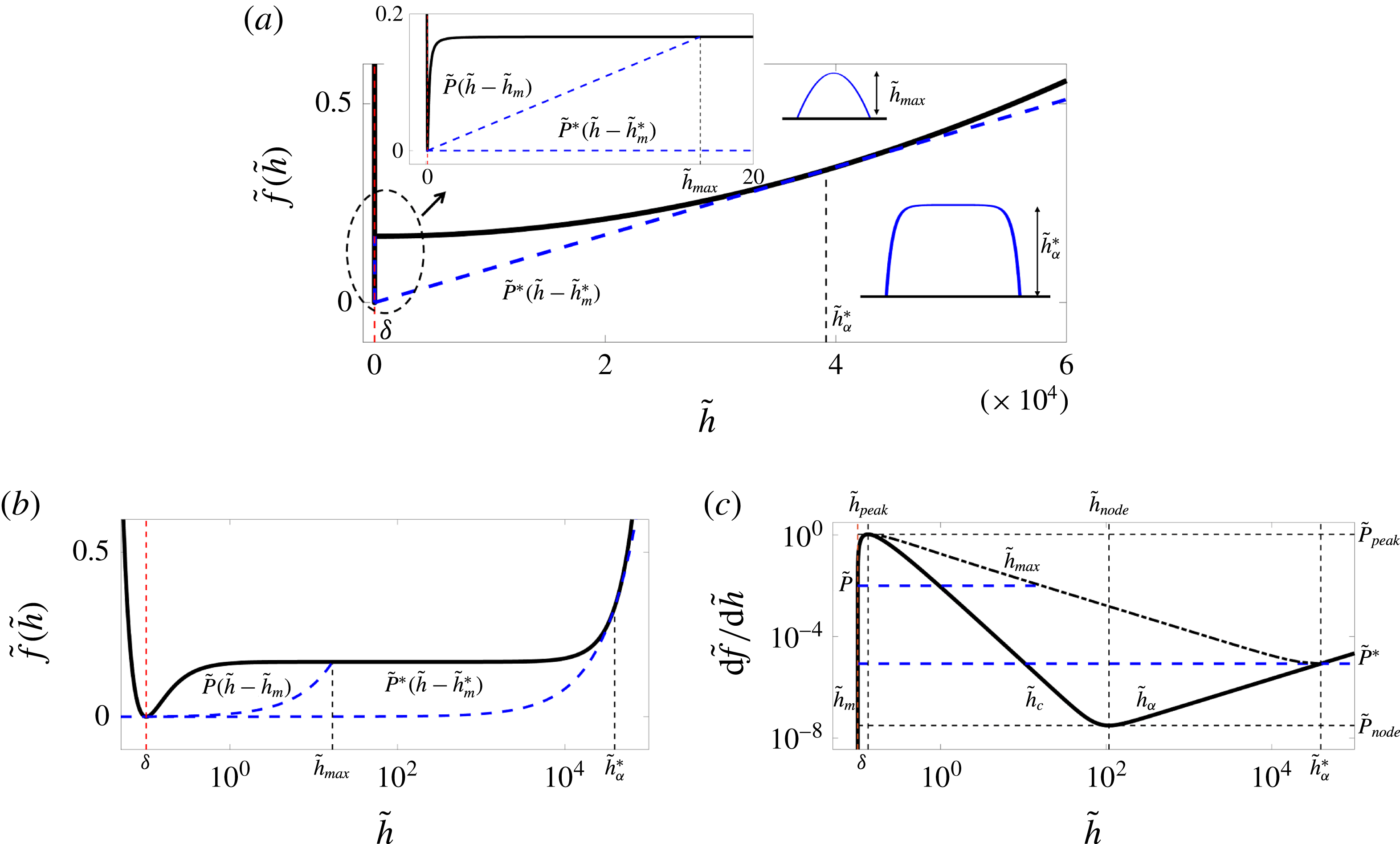
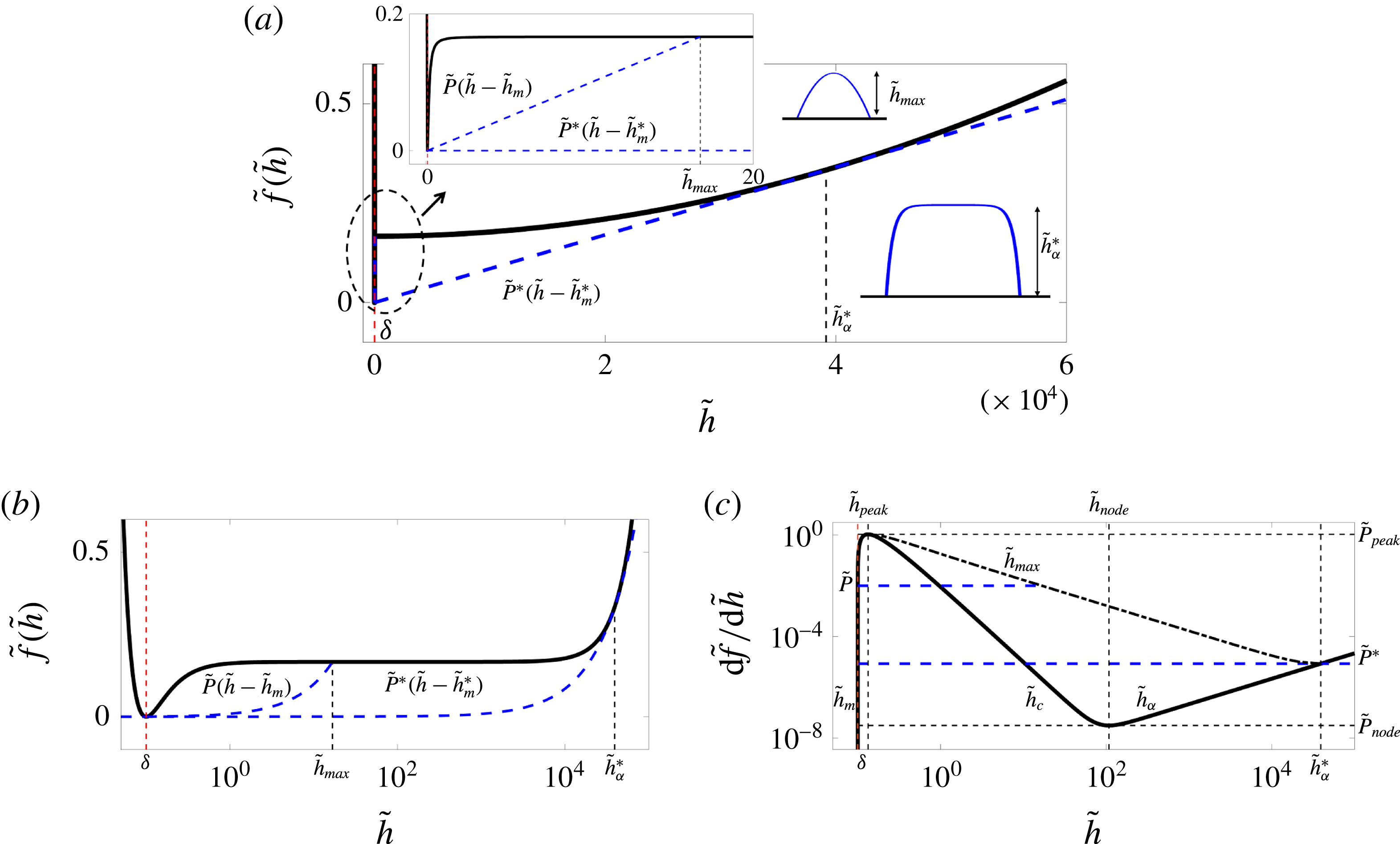
(a) The bulk free energy
 $\tilde{f}(\tilde{h})$
given by (3.1) with
 $Bo=2.2\times 10^{-10}$
and
 $\unicode[STIX]{x1D6FF}=0.1$
(solid line). The blue dashed line shows the Maxwell double-tangent construction, which is tangent to the bulk free energy at
 $\tilde{h}_{m}^{\ast }$
, the precursor film thickness, and at
 $\tilde{h}_{\unicode[STIX]{x1D6FC}}^{\ast }$
, the puddle height. The inset shows a zoomed-in view of the bulk free energy for small heights. Here, an arbitrary line with slope
 $\tilde{P}^{\ast }<\tilde{P}<\tilde{P}_{peak}$
is tangent to the free energy at
 $\tilde{h}_{m}$
and intersects it at
 $\tilde{h}_{max}$
(blue dashed line). (b) The bulk free energy redrawn on a semilog scale. While vdW forces act at nanoscale, gravity only becomes relevant on the millimetre scale; this
 $6$
orders of magnitude separation of scales is shown here. Note that the tangent lines become curved in this semilog representation. (c) The bulk pressure defined as
 $\text{d}\tilde{f}/\text{d}\tilde{h}$
. Droplet solutions exist for
 $\tilde{P}^{\ast }<\tilde{P}<\tilde{P}_{peak}$
, where a typical constant pressure line (
 $\tilde{P}=\text{const.}$
) intersects the curve at three fixed points corresponding to the three branches
 $\tilde{h}_{m}$
,
 $\tilde{h}_{c}$
and
 $\tilde{h}_{\unicode[STIX]{x1D6FC}}$
, as indicated. Uniform films on the
 $\tilde{h}_{c}$
branch are linearly unstable since their corresponding
 $\text{d}^{2}\tilde{f}/\text{d}\tilde{h}^{2}<0$
. The
 $\tilde{h}_{max}$
branch shows the maximum height of the droplet solutions surrounded by a corresponding film of thickness
 $\tilde{h}_{m}$
; these are solutions homoclinic to
 $\tilde{h}_{m}$
, where a line with slope
 $\tilde{P}$
is tangent to the bulk free energy at
 $\tilde{h}_{m}$
and intersects it at
 $\tilde{h}_{max}$
(the blue dashed tangent line). In the limit of very large drops (i.e. puddles)
 $\tilde{h}_{m}$
and
 $\tilde{h}_{max}$
approach
 $\tilde{h}_{m}^{\ast }$
and
 $\tilde{h}_{\unicode[STIX]{x1D6FC}}^{\ast }$
, respectively, and we recover the common tangent line with slope
 $\tilde{P}^{\ast }$
(the blue dashed tangent line) (see also Brochard-Wyart et al.
Reference Brochard-Wyart, Di Meglio, Quere and de Gennes1991; de Gennes et al.
Reference de Gennes, Brochard-Wyart and Quéré2004; Gratton & Witelski Reference Gratton and Witelski2008).
With the above definition of the disjoining pressure, we can now write the bulk free energy as follows:
 $$\begin{eqnarray}\displaystyle & \displaystyle \tilde{f}(\tilde{h})={\displaystyle \frac{1}{2}}Bo\,\tilde{h}^{2}-{\displaystyle \frac{\unicode[STIX]{x1D6FF}^{2}}{\tilde{h}^{2}}}\left({\displaystyle \frac{1}{2}}-{\displaystyle \frac{\unicode[STIX]{x1D6FF}}{3\tilde{h}}}\right)+{\displaystyle \frac{1}{6}}, & \displaystyle\end{eqnarray}$$
where
 $\unicode[STIX]{x1D6FF}=h_{f}/H$
is the non-dimensional precursor film height, and we have chosen
 $L^{2}/H^{2}=\unicode[STIX]{x1D6FE}h_{f}^{2}/{\mathcal{A}}=1/(6(1-\cos \unicode[STIX]{x1D703}_{Y}))$
.
At equilibrium, the thin-film equation (2.19) simplifies to
 $$\begin{eqnarray}\displaystyle & \displaystyle \tilde{P}={\displaystyle \frac{\unicode[STIX]{x1D6FF}\tilde{\unicode[STIX]{x1D6E4}}}{\unicode[STIX]{x1D6FF}\tilde{h}}}={\displaystyle \frac{\text{d}\tilde{f}}{\text{d}\tilde{h}}}-\sqrt{\tilde{\unicode[STIX]{x1D705}}}{\displaystyle \frac{\text{d}}{\text{d}\tilde{x}}}\left(\sqrt{\tilde{\unicode[STIX]{x1D705}}}{\displaystyle \frac{\text{d}\tilde{h}}{\text{d}\tilde{x}}}\right), & \displaystyle\end{eqnarray}$$
where
 $\tilde{P}$
is a constant pressure; the fixed points of the above equation are the solutions of
 $\tilde{P}=\text{d}\tilde{f}/\text{d}\tilde{h}$
. The typical form of the dimensionless free energy
 $\tilde{f}(\tilde{h})$
is shown in figure 2. Within the range
 $\tilde{P}_{node}<\tilde{P}<\tilde{P}_{peak}$
, we can find three fixed points. Using a singular perturbation analysis in the limit
 $\unicode[STIX]{x1D6FF}\rightarrow 0$
, we find these points to be:
 $\tilde{h}_{m}=\unicode[STIX]{x1D6FF}+\unicode[STIX]{x1D6FF}^{2}P+\unicode[STIX]{x1D6FF}^{3}(4P^{2}-Bo)+O(\unicode[STIX]{x1D6FF}^{4})$
,
 $\tilde{h}_{c}=P^{-1/3}\unicode[STIX]{x1D6FF}^{2/3}-(1/3)\unicode[STIX]{x1D6FF}+1/3(BoP^{-5/3}-2/3P^{1/3})\unicode[STIX]{x1D6FF}^{4/3}+O(\unicode[STIX]{x1D6FF}^{5/3})$
and
 $\tilde{h}_{\unicode[STIX]{x1D6FC}}=P/Bo-(Bo^{2}/P^{3})\unicode[STIX]{x1D6FF}^{2}+(Bo^{3}/P^{4})\unicode[STIX]{x1D6FF}^{3}+O(\unicode[STIX]{x1D6FF}^{4})$
, where, to leading order, only the equilibrium film thickness is independent of the pressure. The fixed points obtained here are not affected by the height dependence of the surface tension
 $\tilde{\unicode[STIX]{x1D705}}(\tilde{h})$
as they only depend on the bulk free energy (Gratton & Witelski Reference Gratton and Witelski2008). The pressure in the liquid phase, however, can be affected by the non-constant surface tension, as we will show later; this pressure change will then affect the fixed points.
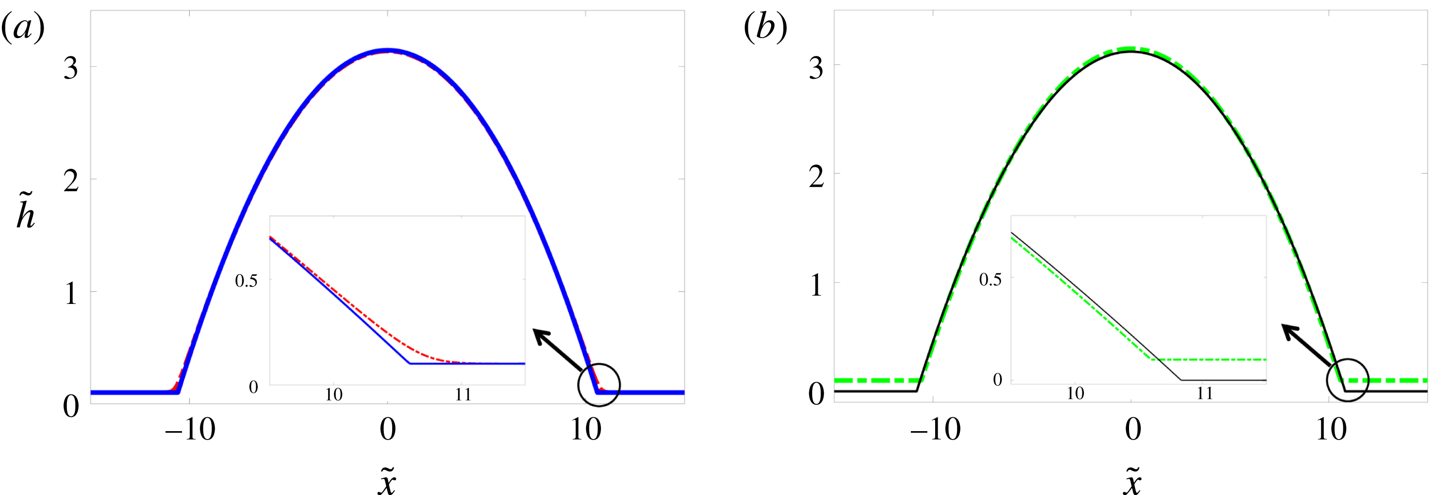
Equilibrium droplet profiles for (a) constant (red dash-dotted line) and height-dependent (solid blue line) surface tension models with a surrounding precursor film, and (b) the height-dependent surface tension model with (green dash-dotted line) and without (solid black line) a surrounding precursor film.
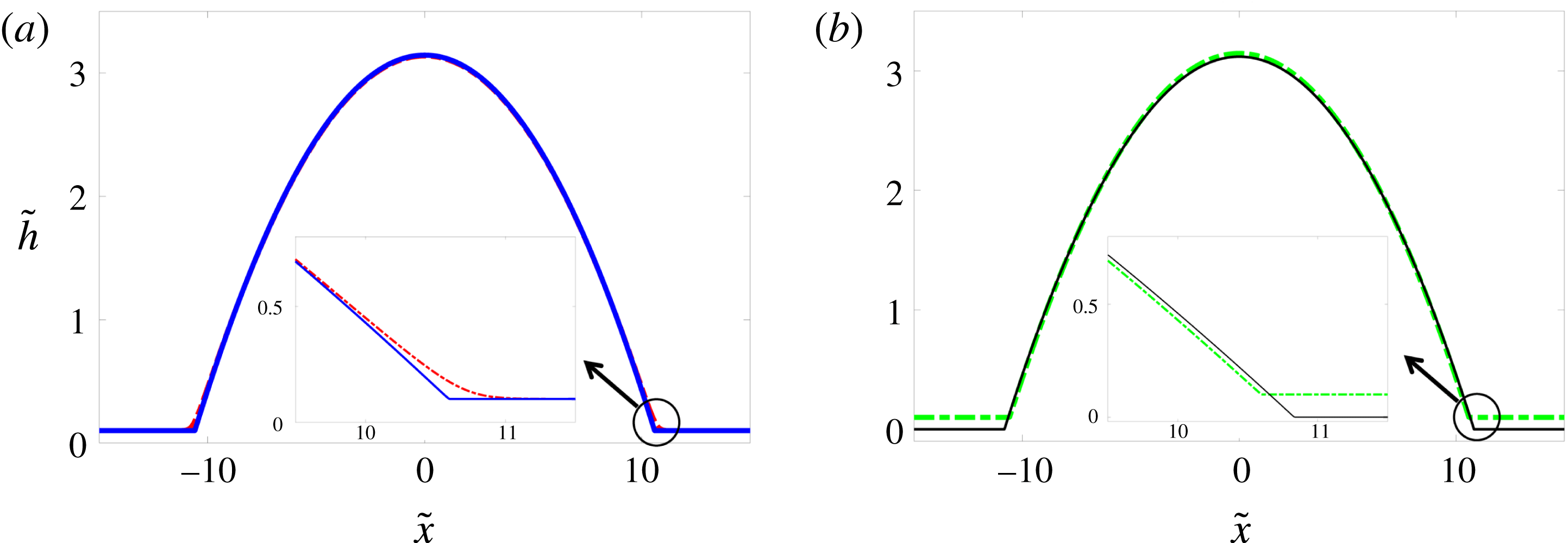
The heights
 $\tilde{h}_{m}$
and
 $\tilde{h}_{\unicode[STIX]{x1D6FC}}$
are saddle points, whereas
 $\tilde{h}_{c}$
is a centre (Gratton & Witelski Reference Gratton and Witelski2008). In the range of
 $\tilde{P}_{node}<\tilde{P}<\tilde{P}_{peak}$
, we can find three types of solutions that are bounded in height (Thiele et al.
Reference Thiele, Velarde, Neuffer and Pomeau2001b
; Gratton Reference Gratton2008): localized hole/dimple solutions that are homoclinic to
 $\tilde{h}_{\unicode[STIX]{x1D6FC}}$
in the range
 $\tilde{P}_{node}<\tilde{P}<\tilde{P}^{\ast }$
, droplet solutions that are homoclinic to
 $\tilde{h}_{m}$
in the range
 $\tilde{P}^{\ast }<\tilde{P}<\tilde{P}_{peak}$
, and heteroclinic orbits from
 $\tilde{h}_{m}$
to
 $\tilde{h}_{\unicode[STIX]{x1D6FC}}$
at
 $\tilde{P}=\tilde{P}^{\ast }$
. To obtain the maximum height of these droplets, we integrate (3.2) as follows:
 $$\begin{eqnarray}\displaystyle & \displaystyle {\mathcal{R}}(\tilde{h})\equiv {\displaystyle \frac{1}{2}}\left(\tilde{\unicode[STIX]{x1D705}}(\tilde{h})\left({\displaystyle \frac{\text{d}\tilde{h}}{\text{d}\tilde{x}}}\right)^{2}\right)=\tilde{f}(\tilde{h})-\tilde{f}(\tilde{h}_{m})-\tilde{P}(\tilde{h}-\tilde{h}_{m}), & \displaystyle\end{eqnarray}$$
where at the maximum height of the drop we have
 $\text{d}\tilde{h}/\text{d}\tilde{x}=0$
, i.e.
 ${\mathcal{R}}(\tilde{h}_{max})=0$
; in the limit
 $\unicode[STIX]{x1D6FF}\rightarrow 0$
, we can then obtain
 $\tilde{h}_{max}=(1/Bo)(\tilde{P}-\sqrt{\tilde{P}^{2}-Bo/3})+(\tilde{P}/\sqrt{\tilde{P}^{2}-Bo/3})\unicode[STIX]{x1D6FF}+O(\unicode[STIX]{x1D6FF}^{2})$
, which is the branch shown in figure 2(c). As the pressure decreases towards
 $\tilde{P}^{\ast }$
, a saddle–saddle heterogeneous orbit appears between
 $\tilde{h}_{m}$
and
 $\tilde{h}_{\unicode[STIX]{x1D6FC}}$
, and the
 $\tilde{h}_{max}$
branch intersects with the
 $\tilde{h}_{\unicode[STIX]{x1D6FC}}$
branch. At this point, we then obtain
 $\tilde{P}^{\ast }=\sqrt{Bo/3}+(Bo/2)\unicode[STIX]{x1D6FF}+O(\unicode[STIX]{x1D6FF}^{2})$
; this critical value of pressure is the slope of the Maxwell common tangent line (Rowlinson & Widom Reference Rowlinson and Widom2013) shown in figure 2 and satisfies the following equations:
 $$\begin{eqnarray}\displaystyle & \displaystyle \tilde{P}^{\ast }={\displaystyle \frac{\tilde{f}(\tilde{h}_{\unicode[STIX]{x1D6FC}}^{\ast })-\tilde{f}(\tilde{h}_{m}^{\ast })}{\tilde{h}_{\unicode[STIX]{x1D6FC}}^{\ast }-\tilde{h}_{m}^{\ast }}}, & \displaystyle\end{eqnarray}$$
 $$\begin{eqnarray}\displaystyle & \displaystyle \tilde{P}^{\ast }=\left.{\displaystyle \frac{\text{d}\tilde{f}}{\text{d}\tilde{h}}}\right|_{\tilde{h}_{m}^{\ast }}=\left.{\displaystyle \frac{\text{d}\tilde{f}}{\text{d}\tilde{h}}}\right|_{\tilde{h}_{\unicode[STIX]{x1D6FC}}^{\ast }}, & \displaystyle\end{eqnarray}$$
 $\tilde{h}_{m}^{\ast }$
and
 $\tilde{h}_{\unicode[STIX]{x1D6FC}}^{\ast }$
are the values of
 $\tilde{h}_{m}$
and
 $\tilde{h}_{\unicode[STIX]{x1D6FC}}$
as calculated at pressure
 $\tilde{P}=\tilde{P}^{\ast }$
.
At
 $\tilde{P}_{node}$
and
 $\tilde{P}_{peak}$
, the
 $\tilde{h}_{c}$
branch merges with the other two branches and we have
 $\text{d}^{2}\tilde{f}/\text{d}\tilde{h}^{2}=0$
. Following the procedure above, in the limit of
 $\unicode[STIX]{x1D6FF}\rightarrow 0$
and using a singular perturbation analysis, we find the corresponding film heights:
 $\tilde{h}_{peak}=(4/3)\unicode[STIX]{x1D6FF}+(4/3)^{5}(Bo/3)\unicode[STIX]{x1D6FF}^{3}+O(\unicode[STIX]{x1D6FF}^{7})$
and
 $\tilde{h}_{node}=(3/Bo)^{1/4}\unicode[STIX]{x1D6FF}^{1/2}-(1/3)\unicode[STIX]{x1D6FF}+O(\unicode[STIX]{x1D6FF}^{2})$
, which lead to the following pressures:
 $\tilde{P}_{peak}=(27/256\unicode[STIX]{x1D6FF})+(4Bo/3)\unicode[STIX]{x1D6FF}+O(\unicode[STIX]{x1D6FF}^{3})$
and
 $\tilde{P}_{node}=4(Bo/3)^{3/4}\unicode[STIX]{x1D6FF}^{1/2}-(Bo/3)\unicode[STIX]{x1D6FF}-2/3(Bo/3)^{5/4}\unicode[STIX]{x1D6FF}^{3/2}+O(\unicode[STIX]{x1D6FF}^{2})$
, which mark the upper and lower boundaries of the pressure range for which equilibrium droplet solutions exist. Note that the results we have obtained so far are only indirectly affected by the height dependence of surface tension through the change of liquid pressure at equilibrium, as we show later.
The droplet solutions of (3.2) can be divided into three regions: (i) core, (ii) contact line and (iii) equilibrium film. Here, we focus on the limit of small drops, where gravity can be neglected (
 $Bo\rightarrow 0$
). In the core (region (i)), away from the contact line and in the absence of intermolecular forces, surface tension is the dominant force, and equation (3.2) simplifies to
 $\tilde{P}=-\tilde{h}_{\tilde{x}\tilde{x}}$
, leading to a parabolic profile,
 $\tilde{h}_{core}=(1/2)\tilde{P}(\tilde{w}^{2}-\tilde{x}^{2})$
, where
 $\tilde{w}$
is the effective width of the droplet. The maximum height of the core region at its centre
 $\tilde{x}=0$
is therefore
 $\tilde{h}_{max}=\tilde{P}\tilde{w}^{2}/2$
. Before, we derived the maximum height of the droplet in the presence of gravity and intermolecular forces. In the limit of zero Bond number, we can then show
 $\tilde{h}_{max}=1/(6\tilde{P})+\unicode[STIX]{x1D6FF}+O(\unicode[STIX]{x1D6FF}^{2})$
; equating this to the maximum height of the parabolic core, we find the effective width of the drop to leading order:
 $\tilde{w}=1/(\sqrt{3}\tilde{P})$
. In the second region (region (ii)), i.e. the region near the contact line, the drop profile asymptotically matches the droplet core to the equilibrium film outside. In this region, we use the following transformation
 $\tilde{h}(\tilde{x})=\unicode[STIX]{x1D6FF}\tilde{H}(\tilde{x})$
with
 $\tilde{x}=-\tilde{w}+\unicode[STIX]{x1D6FF}\tilde{z}$
, and defining
 $\tilde{f}(\tilde{h})\equiv \tilde{F}(\tilde{H})$
we rescale (3.2) to leading order as follows:
 $$\begin{eqnarray}\displaystyle & \displaystyle {\displaystyle \frac{\text{d}\tilde{F}}{\text{d}\tilde{H}}}-\left(1-{\displaystyle \frac{\tilde{F}(\tilde{H})}{\tilde{F}(1)}}\right)\tilde{H}_{\tilde{z}\tilde{z}}+{\displaystyle \frac{1}{2\tilde{F}(1)}}{\displaystyle \frac{\text{d}\tilde{F}}{\text{d}\tilde{H}}}\tilde{H}_{\tilde{z}}^{2}=0, & \displaystyle\end{eqnarray}$$
where we have used the definition
 $\tilde{\unicode[STIX]{x1D705}}=1-\tilde{F}(\tilde{H})/\tilde{F}(1)$
, which appears in the second term. This equation can be integrated to obtain
 $\tilde{H}_{\tilde{z}}^{2}/2=-\tilde{F}(1)$
, relating the slope of the profile in the contact-line region to the intermolecular forces. Consistent with the experimental observations (Pompe & Herminghaus Reference Pompe and Herminghaus2000) and density functional calculations (Snoeijer & Andreotti Reference Snoeijer and Andreotti2008), the height dependence of surface tension leads to a non-zero contact angle at the contact line. In this model the droplet width is a finite value that can be unambiguously defined, where the droplet meets the surrounding wet or dry surface at a non-zero angle (figure 3
b). This is in clear contrast with the classical model with a constant surface tension,
 $\tilde{\unicode[STIX]{x1D705}}=1$
, for which we obtain
 $\tilde{H}_{\tilde{z}}^{2}/2=\tilde{F}(\tilde{H})-\tilde{F}(1)$
, leading to a zero contact angle as the droplet asymptotically meets the precursor film, i.e.
 $\tilde{H}\rightarrow 1$
(figure 3
a). In the classical model, only the macroscopic contact angle far away from the contact line can be non-zero; we therefore need to take the limit of
 $\tilde{H}\rightarrow \infty$
, where
 $\tilde{F}(\tilde{H})\rightarrow 0$
, recovering the result
 $\tilde{H}_{\tilde{z}}^{2}/2=-\tilde{F}(1)$
. Using the dimensional version of this result leads to
 $h_{x}^{2}/2={\mathcal{A}}/(6\unicode[STIX]{x1D6FE}h_{f}^{2})$
, which simplifies to
 $h_{x}^{2}/2=(1-\cos \unicode[STIX]{x1D703}_{Y})$
using the definition
 ${\mathcal{A}}=-6h_{f}^{2}{\mathcal{S}}$
; in the limit of small contact angles (
 $\unicode[STIX]{x1D703}_{Y}\ll 1$
), we can therefore relate the droplet slope to the Young contact angle:
 $h_{x}\approx \unicode[STIX]{x1D703}_{Y}$
.
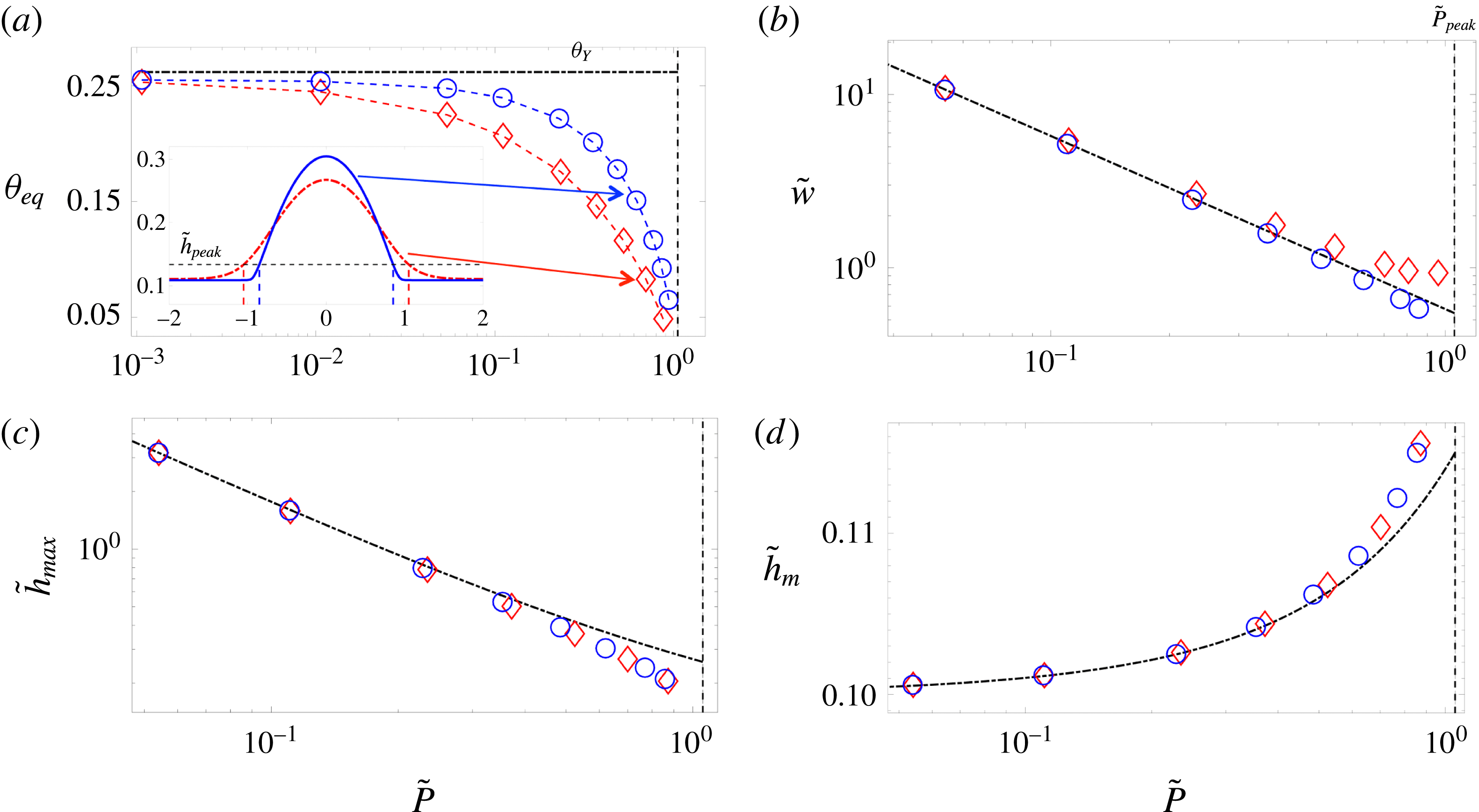
The variation of equilibrium droplet features with the liquid pressure in the droplet. The symbols show the result of numerical simulations with a constant surface tension (red diamonds), and a height-dependent surface tension (blue circles). The dash-dotted lines represent the theoretical predictions for small droplets, and the vertical dashed lines correspond to the
 $\tilde{P}_{peak}$
beyond which no droplet solutions exist. (a) The equilibrium contact angle defined at the inflection point of the droplet profile; the dash-dotted line represents the Young contact angle. The inset shows two typical droplet profiles of equal mass (but different equilibrium pressure, with the new model leading to smaller liquid pressures) for the constant surface tension (red dash-dotted line) and height-dependent surface tension (blue solid line) models. (b) Droplet width defined as the distance from centre of the drop to its edge at
 $\tilde{h}_{peak}$
. The dash-dotted line represents
 $\tilde{w}=1/(\sqrt{3}\tilde{P})$
. In the constant surface tension case, the droplet core asymptotically meets the equilibrium film, leading to a larger effective width. (c) Maximum droplet height. The dash-dotted line represents
 $\tilde{h}_{max}=1/(6\tilde{P})+\unicode[STIX]{x1D6FF}+O(\unicode[STIX]{x1D6FF}^{2})$
. The height dependence of surface tension results in lower equilibrium pressures, which in turn lead to larger
 $\tilde{h}_{max}$
values in the small droplets. (d) Equilibrium film thickness. The dash-dotted line represents
 $\tilde{h}_{m}=\unicode[STIX]{x1D6FF}+\unicode[STIX]{x1D6FF}^{2}P+\unicode[STIX]{x1D6FF}^{3}(4P^{2}-Bo)$
.
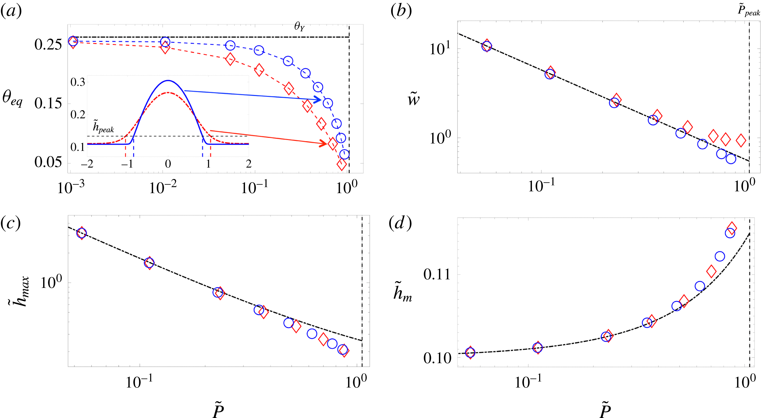
Figure 4 shows the variation of some of the droplet features as a function of its equilibrium pressure (or size) for both the classical model (with constant surface tension) and our model (with a height-dependent surface tension). The first observation is that the difference between the two models is most pronounced for very small droplets, where their entire profile is influenced by the intermolecular forces; as the droplets become larger, intermolecular forces can only be felt very close to the contact line, and the difference between the two models is limited to the vicinity of this region and less relevant to macroscopic features such as width, maximum height, or even equilibrium film thickness, which is now determined by balancing the Laplace pressure due to the curvature of the core region of the drops. The equilibrium contact angle also becomes size-dependent for very small droplets (figure 4
a), where the entire droplet geometry is influenced by the intermolecular forces; this dependence, however, is not due to the line tension effect, which would be relevant for axisymmetric drops (Amirfazli & Neumann Reference Amirfazli and Neumann2004; Schimmele, Napiorkowski & Dietrich Reference Schimmele, Napiorkowski and Dietrich2007; Weijs et al.
Reference Weijs, Marchand, Andreotti, Lohse and Snoeijer2011; Giro et al.
Reference Giro, Bryant, Engel, Neumann and Steiner2017). The second observation is that for small droplets, the height-dependent surface tension model always leads to more localized profiles with larger contact angle and smaller effective width; for equal droplet mass, the height dependence of surface tension leads to a lower equilibrium pressure, which according to the tangent construction shown in figure 2 leads to a larger maximum height (
 $\tilde{h}_{max}$
) and smaller equilibrium film thickness (
 $\tilde{h}_{m}$
).
All the simulations in this paper are performed assuming an equilibrium film thickness of
 $h_{f}=1~\text{nm}$
, and characteristic height
 $H=10~\text{nm}$
, which is the typical range of dominance of vdW forces, leading to a non-dimensional equilibrium film height of
 $\unicode[STIX]{x1D6FF}=h_{f}/H=0.1$
, and
 $Bo=(L/l_{\unicode[STIX]{x1D6FE}})^{2}=2.2\times 10^{-10}$
, i.e. negligible gravity (capillary length
 $l_{\unicode[STIX]{x1D6FE}}=1.5~\text{mm}$
); while the influence of gravity in thin films is in principle insignificant, ignoring its role can lead to unphysical predictions (Thiele et al.
Reference Thiele, Velarde, Neuffer and Pomeau2001b
).
4 Stability of uniform films
Here, we analyse the stability of uniform film solutions of (3.2) to infinitesimal and finite perturbations. Consider a uniform film of thickness
 $\tilde{h}_{0}$
that is perturbed infinitesimally by a superposition of Fourier modes as
 $\tilde{h}=\tilde{h}_{0}+\unicode[STIX]{x1D716}\exp (\unicode[STIX]{x1D6FD}\tilde{t}+\text{i}q\tilde{x})$
, where
 $\unicode[STIX]{x1D6FD}$
is the growth rate of the instability,
 $q=2\unicode[STIX]{x03C0}/\unicode[STIX]{x1D706}$
is the wavenumber, and
 $\unicode[STIX]{x1D716}\ll 1$
. Substituting this decomposition into (2.19) and linearizing it to
 $O(\unicode[STIX]{x1D716})$
, we find
 $$\begin{eqnarray}\displaystyle & \displaystyle \unicode[STIX]{x1D6FD}=\tilde{h}_{0}^{3}\,q^{2}(q_{0}-\tilde{\unicode[STIX]{x1D705}}(\tilde{h}_{0})q^{2}), & \displaystyle\end{eqnarray}$$
where
 $q_{0}=-\text{d}^{2}\tilde{f}/\text{d}\tilde{h}^{2}|_{\tilde{h}_{0}}$
. A uniform film becomes unstable if the growth rate is positive
 $\unicode[STIX]{x1D6FD}>0$
, or
 $q_{0}>\tilde{\unicode[STIX]{x1D705}}(\tilde{h}_{0})q^{2}$
. This implies that wavenumbers
 $q<\sqrt{q_{0}/\tilde{\unicode[STIX]{x1D705}}(\tilde{h}_{0})}$
, or equivalently wavelengths
 $\unicode[STIX]{x1D706}>\unicode[STIX]{x1D706}_{c}=2\unicode[STIX]{x03C0}\sqrt{\tilde{\unicode[STIX]{x1D705}}(\tilde{h}_{0})/q_{0}}$
, will be unstable; surface tension damps the shorter-wavelength deformations. The curve
 $q_{0}=0$
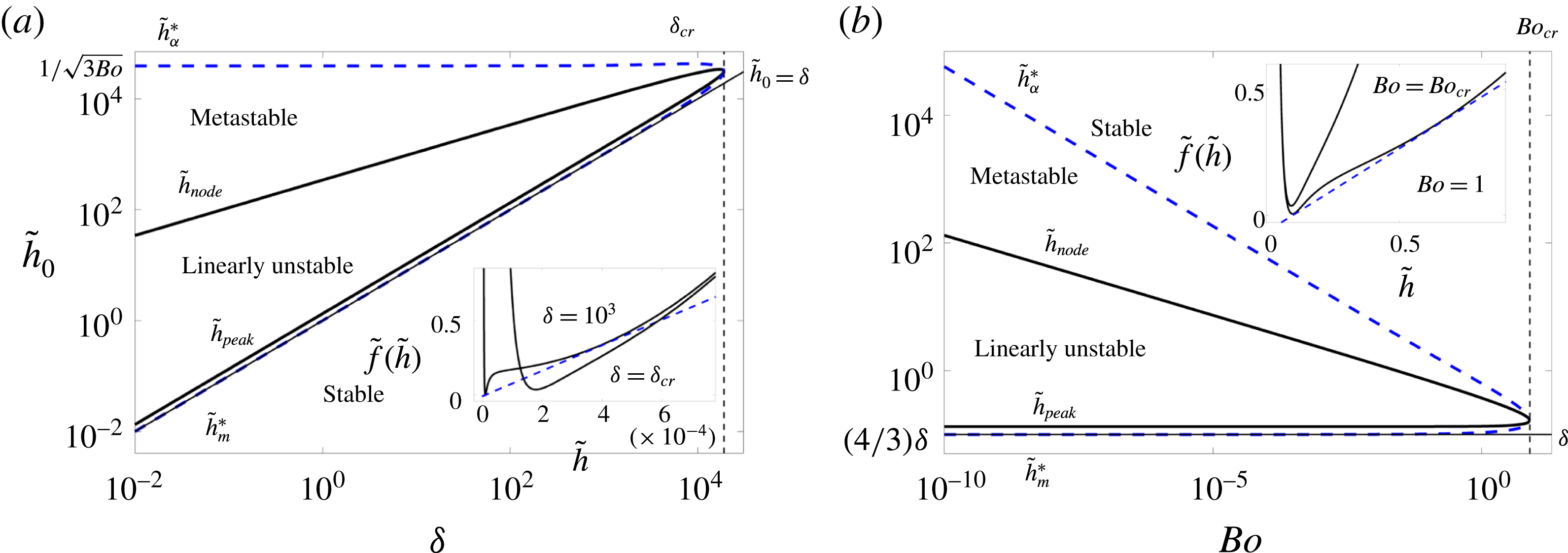
separates the linearly stable and unstable regions, as shown in figure 5; the instability phase diagram can be represented in the phase space of the initial uniform film thickness
 $\tilde{h}_{0}$
versus the equilibrium film thickness
 $\unicode[STIX]{x1D6FF}=h_{f}/H$
(Diez & Kondic Reference Diez and Kondic2007) or
 $\tilde{h}_{0}$
versus
 $Bo$
(Thiele et al.
Reference Thiele, Velarde, Neuffer and Pomeau2001b
). The curve
 $q_{0}=0$
represents the boundary of the spinodal region in the free energy, where the second derivative of the bulk free energy becomes negative,
 $\text{d}^{2}\tilde{f}/\text{d}\tilde{h}^{2}|_{\tilde{h}_{0}}<0$
. This region is bounded by the heights
 $\tilde{h}_{peak}$
and
 $\tilde{h}_{node}$
, as shown in figure 2. The region between these heights and the film heights corresponding to the tangent construction is called the binodal region, where the uniform wetted liquid films are not linearly unstable, but they can be nonlinearly unstable, i.e. if perturbed by a sufficiently large finite-amplitude perturbation they can evolve to find a lower energy state. The boundaries of the binodal region are set by
 $\tilde{h}_{m}^{\ast }$
and
 $\tilde{h}_{\unicode[STIX]{x1D6FC}}^{\ast }$
, as shown in figure 2. The lower and upper branches all meet at a critical point, where the bulk free energy transitions from a double-well to a single-well structure; at the critical point, we have
 $\text{d}^{2}\tilde{f}/\text{d}\tilde{h}^{2}=0$
, and
 $\text{d}^{3}\tilde{f}/\text{d}\tilde{h}^{3}=0$
, leading to
 $\tilde{h}=(5/3)\unicode[STIX]{x1D6FF}$
,
 $\unicode[STIX]{x1D6FF}_{cr}\approx 1.9\times 10^{4}$
, and
 $Bo_{cr}\approx 7.85$
. To find the fastest-growing mode, we take
 $\text{d}\unicode[STIX]{x1D6FD}/\text{d}q=0$
, which leads to the following expressions for the most unstable wavelength
 $$\begin{eqnarray}\displaystyle & \displaystyle \unicode[STIX]{x1D706}_{m}=\sqrt{2}\unicode[STIX]{x1D706}_{c}=2\unicode[STIX]{x03C0}\sqrt{{\displaystyle \frac{2\tilde{\unicode[STIX]{x1D705}}(\tilde{h}_{0})}{-\text{d}^{2}\tilde{f}/\text{d}\tilde{h}^{2}|_{\tilde{h}_{0}}}}}, & \displaystyle\end{eqnarray}$$
and its corresponding maximum growth rate
 $$\begin{eqnarray}\displaystyle & \displaystyle \unicode[STIX]{x1D6FD}_{m}={\displaystyle \frac{\tilde{h}_{0}^{3}}{4\tilde{\unicode[STIX]{x1D705}}(\tilde{h}_{0})}}\left(\left.{\displaystyle \frac{\text{d}^{2}\tilde{f}}{\text{d}\tilde{h}^{2}}}\right|_{\tilde{h}_{0}}\right)^{2}. & \displaystyle\end{eqnarray}$$
Stability phase diagram showing the regions where the uniform film is linearly unstable, metastable (nonlinearly unstable), and absolutely stable. (a) Shows the phase diagram as a function of the initial film height,
 $\tilde{h}_{0}=h_{0}/H$
, and the equilibrium film thickness,
 $\unicode[STIX]{x1D6FF}=h_{f}/H$
. The full black solid line represents the marginal stability curve, where the instability growth rate,
 $\unicode[STIX]{x1D6FD}$
is zero (i.e.
 $q_{0}=-\text{d}^{2}\tilde{f}/\text{d}\tilde{h}^{2}|_{\tilde{h}_{0}}=0$
); inside the curve, the film is linearly unstable to infinitesimal perturbations, whereas outside it is linearly stable; the lower branch of the marginal stability curve is coincident with
 $\tilde{h}_{peak}$
, whereas the upper branch represents
 $\tilde{h}_{node}$
. The blue dashed line represents the curve of absolute stability; outside this curve, all films are absolutely stable, whereas inside it uniform films can become unstable due to finite perturbations, i.e. they are nonlinearly unstable. The upper and lower branches of the absolute stability curve represent the
 $\tilde{h}_{\unicode[STIX]{x1D6FC}}^{\ast }$
and
 $\tilde{h}_{m}^{\ast }$
lines; these are the points tangent to the Maxwell double-tangent construction. In other words, while the curve of marginal stability represents the spinodal region, where
 $\text{d}^{2}\tilde{f}/\text{d}\tilde{h}^{2}|_{\tilde{h}_{0}}\leqslant 0$
, the curve of absolute stability represents the binodal or coexistence curve. The upper and lower branches meet at the critical point, where we have
 $\text{d}^{2}\tilde{f}/\text{d}\tilde{h}^{2}=0$
, and
 $\text{d}^{3}\tilde{f}/\text{d}\tilde{h}^{3}=0$
, leading to
 $\tilde{h}=(5/3)\unicode[STIX]{x1D6FF}$
and
 $\unicode[STIX]{x1D6FF}_{cr}\approx 1.9\times 10^{4}$
, where (as shown in the inset) a transition from a double-well to a single-well structure occurs in the free energy. The dashed blue line in the inset represents the tangent construction. (b) Shows the phase diagram as a function of the initial film thickness,
 $\tilde{h}_{0}$
, and the Bond number
 $Bo$
. The same transition from a double-well to a single-well structure is observed at a critical Bond number of
 $Bo_{cr}\approx 7.85$
where the upper and lower branches of the stability curves meet.
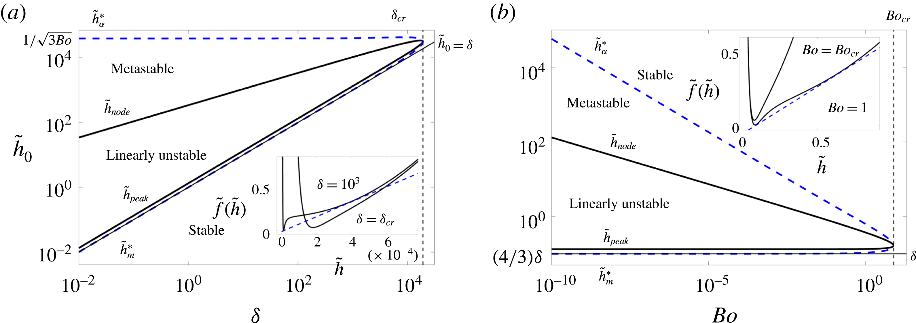
We observe that both the instability wavelength and growth rate are affected by the height dependence of the surface tension. We can denote the corresponding predictions of the classical model by
 $\unicode[STIX]{x1D706}_{m,\unicode[STIX]{x1D705}c}=2\unicode[STIX]{x03C0}\sqrt{1/q_{0}}$
and
 $\unicode[STIX]{x1D6FD}_{m,\unicode[STIX]{x1D705}c}=(\tilde{h}_{0}^{3}/4)q_{0}^{2}$
, where the subscript
 $\unicode[STIX]{x1D705}c$
represents constant surface tension. The new model therefore predicts a smaller instability wavelength,
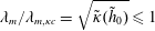 $\unicode[STIX]{x1D706}_{m}/\unicode[STIX]{x1D706}_{m,\unicode[STIX]{x1D705}c}=\sqrt{\tilde{\unicode[STIX]{x1D705}}(\tilde{h}_{0})}\leqslant 1$
, and a faster growth rate
 $\unicode[STIX]{x1D6FD}_{m}/\unicode[STIX]{x1D6FD}_{m,\unicode[STIX]{x1D705}c}=1/\tilde{\unicode[STIX]{x1D705}}(\tilde{h}_{0})\geqslant 1$
, as shown in figure 6. For very large initial thicknesses, the effect of height dependence of surface tension becomes insignificant and both models predict the same scaling for the maximum growth rate
 $\unicode[STIX]{x1D6FD}_{m}\sim \tilde{h}_{0}^{-5}$
(figure 6
b), showing that it drastically reduces as the film thickness increases. The height dependence of surface tension, however, leads to a larger growth rate for small film thicknesses, predicting that the instability grows faster. The largest
 $\unicode[STIX]{x1D6FD}_{m}$
corresponds to
 $\tilde{h}_{0}=(28/15)\unicode[STIX]{x1D6FF}$
for the classical model and
 $\tilde{h}_{0}\approx 1.7\unicode[STIX]{x1D6FF}$
for the new model. Both models predict a similar scaling for the most unstable wavelength at large thicknesses
 $\unicode[STIX]{x1D706}_{m}\sim \tilde{h}_{0}^{2}$
(figure 6
c), whereas for smaller heights, where the effect of variability of surface tension becomes relevant, the new model predicts smaller wavelengths. The minimum
 $\unicode[STIX]{x1D706}_{m}$
corresponds to
 $\tilde{h}_{0}=(5/3)\unicode[STIX]{x1D6FF}$
for the classical model and
 $\tilde{h}_{0}\approx 1.52\unicode[STIX]{x1D6FF}$
for the new model. Note that these heights are different from those concerning the maximum growth rate
 $\unicode[STIX]{x1D6FD}_{m}$
. Further, the instability wavelength shows a much weaker dependence on the film thickness than the growth rate (
 $\tilde{h}_{0}^{2}$
versus
 $\tilde{h}_{0}^{-5}$
). Within the linearly unstable region, the new model predicts the instability can grow up to six times faster than the predictions of the classical model (figure 6
d) while its corresponding instability wavelength can be less than half of that in the classical model; the growth rate is therefore a more sensitive measure of the height dependence of surface tension.
Linear stability analysis results. (a) Dispersion curve showing the instability growth rate
 $\unicode[STIX]{x1D6FD}$
versus the wavenumber
 $q$
for a film of thickness
 $\tilde{h}_{0}=4\unicode[STIX]{x1D6FF}$
. All curves labelled with
 $\unicode[STIX]{x1D705}c$
and
 $\unicode[STIX]{x1D705}(h)$
represent the classical model with a constant surface tension and the new model with a height-dependent surface tension, respectively. The new model results in a shift to larger values for both the maximum growth rate
 $\unicode[STIX]{x1D6FD}_{m}$
and its corresponding wavenumber, leading to a smaller wavelength of instability
 $\unicode[STIX]{x1D706}_{m}$
. (b) Scaling of the maximum growth rate with the thickness of the initial uniform film
 $\tilde{h}_{0}$
. The vertical dashed line
 $(4/3)\unicode[STIX]{x1D6FF}$
represents the lower limit of linear instability. (c) Wavelength of the instability corresponding to the most unstable mode. (d) Ratio of predicted growth rate and instability wavelength between the new model and the classical model. It is apparent that the maximum ratio corresponds to the smallest film thickness
 $\tilde{h}_{0}=(4/3)\unicode[STIX]{x1D6FF}$
where the film is linearly unstable; below the height of
 $\tilde{h}_{0}=(4/3)\unicode[STIX]{x1D6FF}$
the film becomes linearly stable and the surface tension keeps decreasing until it reaches a value of zero for
 $\tilde{h}_{0}=\unicode[STIX]{x1D6FF}$
.
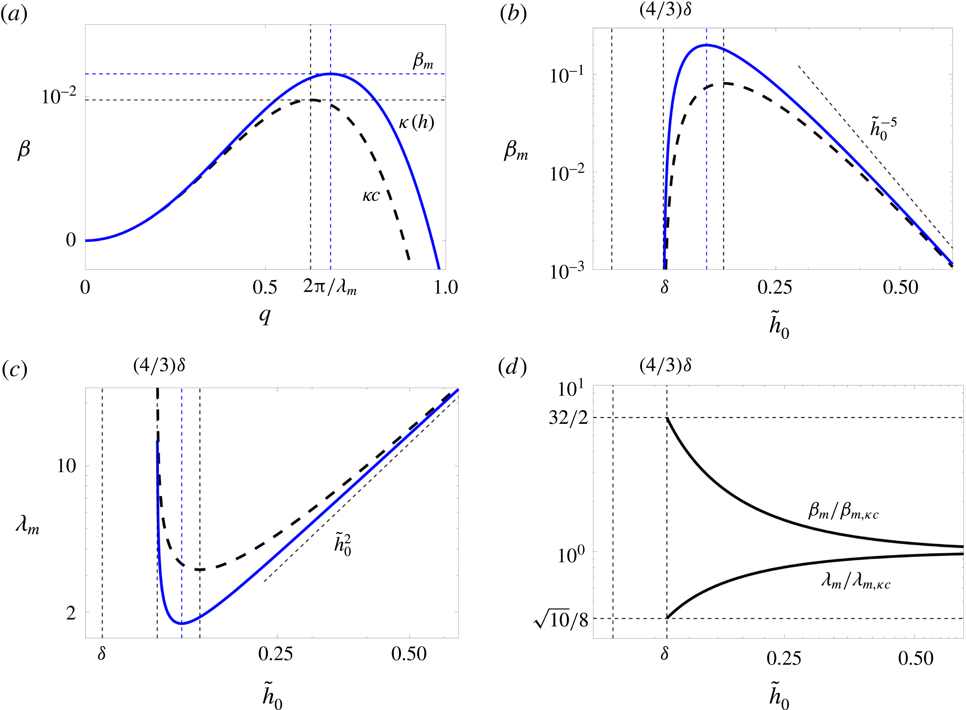
2D simulations of dewetting in the spinodal regime with
 $\tilde{h}_{0}=2\unicode[STIX]{x1D6FF}$
in a domain of size
 $10\unicode[STIX]{x1D706}_{m}$
by
 $10\unicode[STIX]{x1D706}_{m}$
; 2D profiles of
 $\tilde{h}(\tilde{x},{\tilde{y}})$
with contour levels between
 $\tilde{h}_{min}$
and
 $\tilde{h}_{max}$
as specified are shown. (a) The classical thin-film equation (
 $\tilde{h}_{min}=1.99\unicode[STIX]{x1D6FF},1.86\unicode[STIX]{x1D6FF},\unicode[STIX]{x1D6FF},\unicode[STIX]{x1D6FF}$
, and
 $\tilde{h}_{max}=2.02\unicode[STIX]{x1D6FF},2.16\unicode[STIX]{x1D6FF},4\unicode[STIX]{x1D6FF},6.7\unicode[STIX]{x1D6FF}$
, respectively). (b) The stochastic thin-film equation (5.2) with constant surface tension at temperature
 $T=50\,^{\circ }\text{C}$
, i.e.
 $\unicode[STIX]{x1D70E}=0.039$
(
 $\tilde{h}_{min}=\unicode[STIX]{x1D6FF}$
, and
 $\tilde{h}_{max}=2.8\unicode[STIX]{x1D6FF},4.3\unicode[STIX]{x1D6FF},5.1\unicode[STIX]{x1D6FF},7.5\unicode[STIX]{x1D6FF}$
, respectively). (c) The new model with height-dependent surface tension (
 $\tilde{h}_{min}=\unicode[STIX]{x1D6FF}$
, and
 $\tilde{h}_{max}=2.8\unicode[STIX]{x1D6FF},4.3\unicode[STIX]{x1D6FF},5.1\unicode[STIX]{x1D6FF},7.5\unicode[STIX]{x1D6FF}$
, respectively). Both thermal fluctuations and height dependence of surface tension lead to a faster dewetting process, bringing the theoretical predictions closer to the experimental observations (Becker et al.
Reference Becker, Grun, Seemann, Mantz, Jacobs, Mecke and Blossey2003).

The growth of perturbations in the spinodal regime (
 $\tilde{h}_{0}=2\unicode[STIX]{x1D6FF}$
as in figure 7) for the classical model (solid red line), stochastic model (solid green line), and height-dependent surface tension model (solid blue line) as obtained from the nonlinear simulations. The imposed perturbations become damped at early times due to the surface tension, but then start to grow exponentially (as shown by the dashed lines).
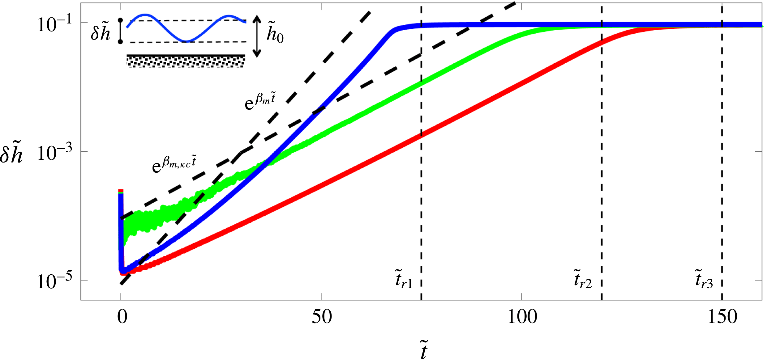
The ratio of the rupture times between the classical model (
 $t_{r,\unicode[STIX]{x1D705}c}$
) and the classical model with thermal noise (green squares), the height-dependent surface tension model without noise (blue circles) and the height-dependent surface tension model with noise (cyan diamonds). Both the thermal noise and height dependence of surface tension lead to a faster rupture time compared to the classical model. While the effect of noise is almost independent of the initial film thickness (green squares), the height dependence of surface tension leads to an increasingly faster ruptures as the film thickness decreases (blue circles). This effect becomes even more amplified when thermal noise is added to the new model (cyan diamonds). The solid line represents the ratio of the growth rates between the classical and new model as predicted from the linear stability analysis (see figure 6
d).
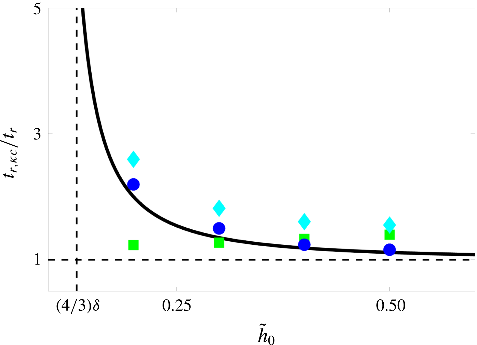
To go beyond the linear stability analysis, we conducted two-dimensional (2D) numerical simulations in the spinodal regime to examine the dewetting rate and morphologies obtained. Figure 7 shows that thermal fluctuations (see equation (5.2)) and height dependence of surface tension both lead to a faster initial dewetting. Figure 8 shows the growth of perturbations in the nonlinear simulations of dewetting using the different models. The linear stability analysis for this film thickness predicts that the growth rate of the height-dependent surface tension model is twice as fast as the classical model (
 $\unicode[STIX]{x1D6FD}_{m}/\unicode[STIX]{x1D6FD}_{m,\unicode[STIX]{x1D705}c}=2$
). From the nonlinear simulations we find that the new model leads to a film rupture at
 $\tilde{t}_{r1}\approx 75$
, whereas the classical model leads to a rupture time of
 $\tilde{t}_{r3}\approx 150$
, which is in agreement with the linear stability predictions. Thermal fluctuations at
 $T=50\,^{\circ }\text{C}$
, i.e.
 $\unicode[STIX]{x1D70E}=0.039$
(see equation (5.2)), lead to a rupture around
 $\tilde{t}_{r2}\approx 125$
, which is faster than the classical model. Figure 9 shows a more quantitative comparison of the rupture times between the classical model and the other models. The speed up observed due to the thermal noise is independent of the initial height of the film, whereas the height dependence of surface tension in the new model leads to increasingly faster rupture as the initial film height decreases. The prediction of a faster growth rate in our model deserves special attention. Earlier studies have pointed to temporal inconsistencies between theoretical predictions and experimental observations (Becker et al.
Reference Becker, Grun, Seemann, Mantz, Jacobs, Mecke and Blossey2003), with experiments showing a faster initial dewetting process by more than a factor of two compared to the theoretical predictions. Our new model therefore brings theoretical predictions closer to the earlier experimental observations. Our results in figure 9 further suggest that to disentangle the roles played by the height dependence of surface tension and the thermal noise, experiments with different initial heights need to be conducted.
5 Coarsening: self-similar intermediate asymptotics
5.1 Coarsening phase diagram
The drops formed after the dewetting process are in a metastable state; they can still communicate through the ultrathin films connecting them and thus coarsen in time to lower the overall energy of the system. Multiplying both sides of (2.19) by
 $\unicode[STIX]{x1D6FF}\unicode[STIX]{x1D6E4}/\unicode[STIX]{x1D6FF}\tilde{h}$
, integrating in space and using the no-flux boundary conditions, we can easily show (see also Thiele et al. (Reference Thiele, Velarde, Neuffer and Pomeau2001b
), Glasner & Witelski (Reference Glasner and Witelski2003)):
 $$\begin{eqnarray}\displaystyle {\displaystyle \frac{\text{d}\unicode[STIX]{x1D6E4}}{\text{d}\tilde{t}}}=-\int {\mathcal{M}}\left({\displaystyle \frac{\unicode[STIX]{x2202}}{\unicode[STIX]{x2202}\tilde{x}}}\left({\displaystyle \frac{\unicode[STIX]{x1D6FF}\unicode[STIX]{x1D6E4}}{\unicode[STIX]{x1D6FF}\tilde{h}}}\right)\right)^{2}\text{d}\tilde{x}\leqslant 0, & & \displaystyle\end{eqnarray}$$
demonstrating that the evolution governed by the thin-film equation leads to a decreasing free energy and, therefore, a thermodynamically admissible system.
Space–time diagrams showing the evolution of drop height of the classical thin-film equation (constant surface tension); the results of the height-dependent case are similar. The simulations are done in a domain of size
 $100\unicode[STIX]{x1D706}_{m}$
and the frames shown here show a zoom-in of a size
 $40\unicode[STIX]{x1D706}_{m}$
. In all the cases, a line coming to an end indicates an Ostwald-ripening event, in which a smaller drop feeds into larger neighbouring drops through the ultrathin film that connects them. (a)
 $\tilde{h}_{0}=4\unicode[STIX]{x1D6FF}$
, representing the classical spinodal regime, where the number of drops is approximately set by the most unstable wavelength
 $\unicode[STIX]{x1D706}_{m}$
(
 $\tilde{h}_{max}=35\unicode[STIX]{x1D6FF}$
). (b)
 $\tilde{h}_{0}=10\unicode[STIX]{x1D6FF}$
representing a mixed-mode instability regime in between spinodal and nucleation regimes; here, fewer drops than the spinodal regime form and the distance between the formed drops seems to be random (
 $\tilde{h}_{max}=100\unicode[STIX]{x1D6FF}$
). (c)
 $\tilde{h}_{0}=25\unicode[STIX]{x1D6FF}$
, which is deep into the nucleation regime, showing the formation of very few drops (
 $\tilde{h}_{max}=700\unicode[STIX]{x1D6FF}$
). (d)
 $\tilde{h}_{0}=4\unicode[STIX]{x1D6FF}$
and including thermal fluctuations (
 $T=50\,^{\circ }\text{C}$
, i.e.
 $\unicode[STIX]{x1D70E}=0.039$
) (
 $\tilde{h}_{max}=25\unicode[STIX]{x1D6FF}$
); thermal noise enhances the lateral motion of the drops; the coarsening mechanism, however, still seems to be dominated by Ostwald ripening.

Figure 10 shows space–time diagrams of the dewetting of thin liquid films of different thickness and their coarsening over time. The simulations presented here are conducted on a large domain of size
 $100\unicode[STIX]{x1D706}_{m}$
and the frames shown are a zoomed-in view of a window of size
 $40\unicode[STIX]{x1D706}_{m}$
; these simulations show the results corresponding to the classical model with a constant surface tension; the results of the height-dependent surface tension model are very similar. In all cases we start with a uniform film of thickness
 $\tilde{h}_{0}$
on which random perturbations of amplitude
 $10^{-4}\tilde{h}_{0}$
are imposed. While all the initial thicknesses are within the linearly unstable regime (see figure 5), they lead to entirely different morphologies.
For small initial film height of
 $\tilde{h}_{0}=4\unicode[STIX]{x1D6FF}$
, we observe the characteristics of the spinodal dewetting, a term originally coined by Mitlin (Reference Mitlin1993) due to its similarity to the spinodal decomposition in binary mixtures (Cahn Reference Cahn1961). In this regime, the distance between the drops is the same as the most unstable wavelength, i.e. we get
 ${\approx}100$
drops in a domain of size
 $100\unicode[STIX]{x1D706}_{m}$
(Diez & Kondic Reference Diez and Kondic2007). The coarsening here proceeds through Ostwald ripening (Ostwald Reference Ostwald1897), or collapse of smaller drops at the expense of growth of larger ones (Glasner & Witelski Reference Glasner and Witelski2003).
As the initial film height increases to
 $\tilde{h}_{0}=10\unicode[STIX]{x1D6FF}$
, we can immediately see in figure 10(b) that the number of drops formed upon dewetting and their spacing no longer follows the predictions of the linear stability analysis, i.e. fewer drops form and their spacing becomes random. This behaviour has signatures of nucleation dewetting within the linearly unstable regime (Thiele, Velarde & Neuffer Reference Thiele, Velarde and Neuffer2001a
; Thiele et al.
Reference Thiele, Velarde, Neuffer and Pomeau2001b
; Diez & Kondic Reference Diez and Kondic2007) and shows a mixed-mode instability, i.e. a behaviour in between spinodal and nucleation regimes. Such a transition has also been reported in phase separation dynamics within the Cahn–Hilliard framework (Novick-Cohen Reference Novick-Cohen1985). Figure 11 shows corresponding 2D simulations of dewetting in this regime; in contrast with the spinodal regime, where holes appear around the same time with a uniform spacing, here the nucleation process begins with formation of a hole, which then laterally expands and forms a rim behind it (Seemann, Herminghaus & Jacobs Reference Seemann, Herminghaus and Jacobs2001b
; Fetzer et al.
Reference Fetzer, Jacobs, Münch, Wagner and Witelski2005; Seemann et al.
Reference Seemann, Herminghaus, Neto, Schlagowski, Podzimek, Konrad, Mantz and Jacobs2005; Bäumchen & Jacobs Reference Bäumchen and Jacobs2010; Bäumchen et al.
Reference Bäumchen, Marquant, Blossey, Münch, Wagner and Jacobs2014). In this mixed-mode regime, the growth rate is still large enough that shortly after growth of a hole, the depression behind the dewetting rim can lead to rupture; this behaviour leads to the satellite-hole formation observed in the experiments (Becker et al.
Reference Becker, Grun, Seemann, Mantz, Jacobs, Mecke and Blossey2003; Neto et al.
Reference Neto, Jacobs, Seemann, Blossey, Becker and Grün2003) and in the 2D simulations of figure 11. Figure 12 illustrates this nucleation process in a space–time diagram of a one-dimensional (1D) simulation of the height-dependent surface tension model with
 $\tilde{h}_{0}=10\unicode[STIX]{x1D6FF}$
.
Nucleation dewetting for
 $\tilde{h}_{0}=10\unicode[STIX]{x1D6FF}$
for the constant surface tension model. In this regime, holes randomly appear and start expanding laterally, forming a growing rim behind them (
 $\tilde{h}_{max}=30\unicode[STIX]{x1D6FF},54\unicode[STIX]{x1D6FF},70\unicode[STIX]{x1D6FF},120\unicode[STIX]{x1D6FF}$
, respectively). The depression behind the dewetting rim leads to the formation of satellite holes. The dewetting rims subsequently become unstable and lead to fingering and pinch off to form droplets (see Reiter & Sharma (Reference Reiter and Sharma2001), Bäumchen et al. (Reference Bäumchen, Marquant, Blossey, Münch, Wagner and Jacobs2014) for experimental details).

As we keep increasing the initial film thickness further to
 $\tilde{h}_{0}=25\unicode[STIX]{x1D6FF}$
(figure 10
c), we move deeper into the nucleation regime, where fewer drops form; in this case five drops formed in random locations in a domain of size
 $40\unicode[STIX]{x1D706}_{m}$
. In the nucleation regime two time scales compete: the time scale associated with the growth of linearly unstable modes and the time scale associated with the dewetting front (Thiele et al.
Reference Thiele, Velarde and Neuffer2001a
; Diez & Kondic Reference Diez and Kondic2007; Snoeijer & Eggers Reference Snoeijer and Eggers2010). As we showed before, the growth rate of the most unstable mode
 $\unicode[STIX]{x1D6FD}_{m}$
scales as
 $\tilde{h}_{0}^{-5}$
, leading to significant decreases in the growth rate for thicker films, thereby favouring growth via nucleation.
Since the dynamics of the coarsening process is slaved to the flux through the ultrathin equilibrium films (
 $\tilde{h}_{m}\approx \unicode[STIX]{x1D6FF}$
) connecting the drops and the mobility scales as
 $\tilde{h}^{3}$
, the coarsening dynamics are extremely slow. Two time scales are involved in this process: a fast time scale over which individual coarsening events happen, and a slow time scale between the individual events (Glasner & Witelski Reference Glasner and Witelski2003). A full numerical simulation of the thin-film equation therefore can be computationally very expensive. Glasner & Witelski (Reference Glasner and Witelski2003) used the separation of time scales in this problem to reduce the governing partial differential equation, equation (2.19), to a system of ordinary differential equations for the droplet pressures and locations. Coarsening can proceed via two general mechanisms: coalescence of droplets or Ostwald ripening (Glasner & Witelski Reference Glasner and Witelski2005). Their mathematical model allowed them to simulate the coarsening of a very large number (
 $O(10^{5})$
) of drops. They observed a scaling of
 $N\sim \tilde{t}^{-2/5}$
for the number of drops in time and also observed a transition from Ostwald-ripening-dominated (capillary-driven drainage and collapse) coarsening to coalescence-dominated coarsening as they increased the total mass of liquid in the domain.
Space–time diagram of the nucleation process in the height-dependent surface tension model with
 $\tilde{h}_{0}=10\unicode[STIX]{x1D6FF}$
in a domain of size
 $20\unicode[STIX]{x1D706}_{m}$
(each snapshot is shifted up by
 $10\unicode[STIX]{x1D6FF}=1$
). The lateral expansion of holes, growth of the rim behind the hole, and the subsequent instability of the dip behind a growing rim can all be seen in this illustration.

In contrast with the findings of Glasner & Witelski (Reference Glasner and Witelski2005), we do not observe such a transition from Ostwald-ripening-dominated to coalescence-dominated coarsening (figure 10). The change in the instability mode from spinodal to nucleation leads to the formation of fewer drops as the total mass of the liquid in the domain increases, i.e. as the initial film height increases: the large distance between the drops favours coarsening through Ostwald ripening rather than coalescence. The reason Glasner & Witelski (Reference Glasner and Witelski2005) observe such a transition is that they keep the number of drops within a given domain fixed as they increase their mass; this naturally leads to wider drops that progressively get closer to each other, therefore favouring coalescence.
5.2 Influence of thermal fluctuations
Some experiments on thin-film dewetting (Limary & Green Reference Limary and Green2002, Reference Limary and Green2003) and nanoparticle growth in thin films (Meli & Green Reference Meli and Green2008; Woehl et al. Reference Woehl, Park, Evans, Arslan, Ristenpart and Browning2014) have reported a crossover from diffusion-dominated to coalescence-dominated behaviour. A potential source of this transition could be thermal noise, which may play a dominant role in thin-film systems (Mecke & Rauscher Reference Mecke and Rauscher2005; Grün et al. Reference Grün, Mecke and Rauscher2006; Fetzer et al. Reference Fetzer, Rauscher, Seemann, Jacobs and Mecke2007b ; Willis & Freund Reference Willis and Freund2009; Belardinelli et al. Reference Belardinelli, Sbragaglia, Gross and Andreotti2016; Diez, González & Fernández Reference Diez, González and Fernández2016). To explore this possibility, we generalize the thin-film equation (2.19) by incorporating thermal noise:
 $$\begin{eqnarray}\displaystyle & \displaystyle {\displaystyle \frac{\unicode[STIX]{x2202}\tilde{h}}{\unicode[STIX]{x2202}\tilde{t}}}={\displaystyle \frac{\unicode[STIX]{x2202}}{\unicode[STIX]{x2202}\tilde{x}}}\left(\tilde{h}^{3}{\displaystyle \frac{\unicode[STIX]{x2202}\tilde{P}}{\unicode[STIX]{x2202}\tilde{x}}}\right)+\unicode[STIX]{x1D70E}{\displaystyle \frac{\unicode[STIX]{x2202}}{\unicode[STIX]{x2202}\tilde{x}}}(\tilde{h}^{3/2}\tilde{\unicode[STIX]{x1D709}}(\tilde{x},\tilde{t})), & \displaystyle\end{eqnarray}$$
in which
 $\tilde{P}=\text{d}\tilde{f}/\text{d}\tilde{h}-\sqrt{\tilde{\unicode[STIX]{x1D705}}}\unicode[STIX]{x2202}/\unicode[STIX]{x2202}\tilde{x}(\sqrt{\tilde{\unicode[STIX]{x1D705}}}\unicode[STIX]{x2202}\tilde{h}/\unicode[STIX]{x2202}\tilde{x})$
, with
 $\tilde{\unicode[STIX]{x1D705}}=\unicode[STIX]{x1D705}/\unicode[STIX]{x1D6FE}$
and
 $\tilde{f}=f/(\unicode[STIX]{x1D6FE}H^{2}/L^{2})$
, where
 $H$
and
 $L$
are characteristic height and length scales. The second term on the right-hand side of the equation represents the thermal fluctuations (Davidovitch, Moro & Stone Reference Davidovitch, Moro and Stone2005; Mecke & Rauscher Reference Mecke and Rauscher2005; Grün et al.
Reference Grün, Mecke and Rauscher2006) with
 $\unicode[STIX]{x1D70E}=\sqrt{k_{B}T/\unicode[STIX]{x1D6FE}H^{2}}$
, where
 $k_{B}$
is Boltzmann’s constant,
 $T$
represents absolute temperature and
 $\tilde{\unicode[STIX]{x1D709}}$
represents a spatiotemporal Gaussian white noise:
 $\langle \tilde{\unicode[STIX]{x1D709}}\rangle =0$
and
 $\langle \tilde{\unicode[STIX]{x1D709}}(\tilde{x},\tilde{t})\tilde{\unicode[STIX]{x1D709}}(\tilde{x}^{\prime },\tilde{t}^{\prime })\rangle =\unicode[STIX]{x1D6FF}(\tilde{x}-\tilde{x}^{\prime })\unicode[STIX]{x1D6FF}(\tilde{t}-\tilde{t}^{\prime })$
with
 $\unicode[STIX]{x1D6FF}$
as the Dirac delta function and
 $\langle .\rangle$
implying ensemble average over realizations of the noise.
Introducing thermal noise to the system leads to enhanced lateral motion of the drops, as seen in figure 10(d), and this can promote coalescence. Our simulations for the stochastic thin-film equation (5.2) within the spinodal regime, however, show the dominance of Ostwald ripening despite the enhanced lateral motion of the drops. The crossover from the diffusion-dominated to coalescence-dominated behaviour observed in the experiments (Limary & Green Reference Limary and Green2002, Reference Limary and Green2003) therefore could be a consequence of the dimensionality of the problem, i.e. 2D in the experiments versus 1D in the simulations shown in figure 10. In two dimensions, each drop can be surrounded and interact with multiple other drops, whereas in one dimension each drop only interacts with its two neighbours. To investigate this, we have conducted 2D nonlinear simulations, which point to the dominance of coalescence events at short times and Ostwald ripening at long times, as shown in figure 13, which corresponds to the height-dependent surface tension model; similar results are obtained for both the classical and stochastic models. Our observations are in agreement with the 2D simulations of Glasner (Reference Glasner2008) using a reduced-order model that suggest the dominance of the coalescence mechanism.
Two-dimensional simulations of coarsening dynamics at early and late times for the height-dependent surface tension model with
 $\tilde{h}_{0}=2\unicode[STIX]{x1D6FF}$
(
 $\tilde{h}_{max}=8.5\unicode[STIX]{x1D6FF}$
in the colourbar). At early times, coalescence events, as highlighted by the dashed white circles, are dominant. At late times (once the metastable drops have formed), however, Ostwald ripening, i.e. capillary drainage and collapse of drops, becomes the key coarsening mechanism; note that this latter process is diffusion-dominated and therefore much slower than coarsening through coalescence events.

Coarsening statistics; red circles and squares correspond to the classical model with
 $\tilde{h}_{0}=4\unicode[STIX]{x1D6FF}$
and
 $\tilde{h}_{0}=10\unicode[STIX]{x1D6FF}$
, respectively; blue diamonds show the results of the new model with
 $\tilde{h}_{0}=4\unicode[STIX]{x1D6FF}$
; green stars correspond to the stochastic thin-film model with
 $\tilde{h}_{0}=4\unicode[STIX]{x1D6FF}$
. (a) Evolution of the number of drops in time shows the scaling
 $\tilde{t}^{-2/5}$
as suggested by Glasner & Witelski (Reference Glasner and Witelski2003). (b) Evolution of mean width of drops in time; as expected from conservation of mass and the scaling of the number of drops in time, the mean width scales as
 $\tilde{t}^{1/5}$
in time. (c) Evolution of the total energy in time shows a decrease in the energy with coarsening with a scaling of
 $\tilde{t}^{-1/5}$
, which is expected for the 1D case (Otto, Rump & Slepcev Reference Otto, Rump and Slepcev2006); the
 $\tilde{h}_{0}=10\unicode[STIX]{x1D6FF}$
case results in fewer drops upon dewetting, therefore the majority of the domain is covered by the equilibrium film, which means the initial energy is lower than the
 $\tilde{h}_{0}=4\unicode[STIX]{x1D6FF}$
case; at long times the dynamics becomes self-similar and both follow the same scaling. (d) Evolution of the bulk
 $E_{b}$
, interfacial
 $E_{i}$
and total
 $E_{t}=E_{b}+E_{i}$
energies for a typical simulation (here
 $\tilde{h}_{0}=4\unicode[STIX]{x1D6FF}$
and height-dependent surface tension model); at short times, creation of drops increases the interfacial energy, but the total energy is still lowered due to the reduction in the bulk energy; at long times, as drops coarsen, both the bulk and interfacial energy contribution decrease.

5.3 Coarsening statistics
The statistics of the coarsening process for (i) the spinodal regime,
 $\tilde{h}_{0}=4\unicode[STIX]{x1D6FF}$
(for both constant and height-dependent surface tension models as well as the classical stochastic thin-film equation with thermal noise) and (ii) for the mixed-mode instability regime
 $\tilde{h}_{0}=10\unicode[STIX]{x1D6FF}$
(for the constant surface tension model) are shown in figure 14. In the spinodal regime, the number of drops follows the scaling
 $N\sim \tilde{t}^{-2/5}$
in time (figure 14
a) as computed by Glasner & Witelski (Reference Glasner and Witelski2003); incorporating the height dependence of surface tension does not alter this scaling. Introducing thermal noise does not affect the scaling either – an observation that is consistent with recent studies (Nesic et al.
Reference Nesic, Cuerno, Moro and Kondic2015). In the mixed-mode instability regime (
 $\tilde{h}_{0}=10\unicode[STIX]{x1D6FF}$
), fewer drops form, so our simulations have limited statistics and do not clearly reach the self-similar intermediate regime (Gratton & Witelski Reference Gratton and Witelski2009), but it seems that the results for this case are also in general agreement with the
 $\tilde{t}^{-2/5}$
scaling (figure 14
a). Due to mass conservation, it is easy to show that the mean width of drops should then follow the scaling
 $\tilde{t}^{1/5}$
, as shown in figure 14(b). An interesting feature of the variation of the mean width in time, particularly at late times, is the jumps observed as smaller drops shrink and feed into the larger drops.
As argued above, the thin-film evolution equation predicts a monotonically decreasing free energy for the system (equation (5.1)). We can further check this by looking at the variation of the numerically calculated total energy of the system
 $E_{t}\equiv \unicode[STIX]{x1D6E4}=\int \tilde{f}(\tilde{h})+(\tilde{\unicode[STIX]{x1D705}}/2)(\tilde{h}_{x})^{2}\,\text{d}\tilde{x}$
. In agreement with the predictions of Otto et al. (Reference Otto, Rump and Slepcev2006), we find a
 $\tilde{t}^{-1/5}$
scaling for the decrease of the free energy (figure 14
c). An interesting observation here is that for the thicker film of
 $\tilde{h}_{0}=10\unicode[STIX]{x1D6FF}$
, we observe a lower total free energy at early times that later converges to the
 $\tilde{t}^{-1/5}$
scaling. To understand the reason behind the difference at early times, it is instructive to look at the typical variation of the different components of the free energy during the entire dewetting process, as shown in figure 14(d). Here,
 $E_{b}=\int \tilde{f}(\tilde{h})\,\text{d}\tilde{x}$
is the bulk free energy and
 $E_{i}=\int (\tilde{\unicode[STIX]{x1D705}}(\tilde{h})/2)(\tilde{h}_{x})^{2}\,\text{d}\tilde{x}$
is the interfacial energy. As an initially uniform film becomes unstable, it must increase the interfacial energy to dewet and create droplets. This increase in the interfacial energy, however, is compensated by the reduction in the bulk free energy as the ultrathin films connecting the drops are in their near-equilibrium states. The drops connected by these ultrathin films, however, are only metastable and, after a long intermediate plateau state, the system starts lowering its total energy through coarsening, which lowers both the interfacial energy as well as the bulk free energy due to the creation of new ultrathin films. With this observation in mind, we can now go back to figure 14(c); here, the thicker film (
 $\tilde{h}_{0}=10\unicode[STIX]{x1D6FF}$
) leads to the formation of fewer drops upon dewetting, meaning lower interfacial and bulk free energies in the mixed-mode instability regime compared to the spinodal regime (formation of fewer drops means a higher fraction of the total surface is covered by the ultrathin films that have a lower bulk free energy). This is why, right after dewetting, the thicker film case
 $\tilde{h}_{0}=10\unicode[STIX]{x1D6FF}$
leads to a lower total free energy compared to the
 $\tilde{h}_{0}=4\unicode[STIX]{x1D6FF}$
case in the spinodal regime. At long times, however, as the coarsening sets in, the dynamics become self-similar and the total system energies per unit length of the substrate corresponding to the different regimes all collapse on top of each other.
5.4 LSW mean-field description of coarsening: self-similar drop-size distribution
In the late stages of a first-order phase transition of a binary alloy mixture, Ostwald ripening is quite common (Ostwald Reference Ostwald1897; Siggia Reference Siggia1979; Voorhees Reference Voorhees1985). The curvature dependence of the chemical potential leads to a flow from higher-curvature regions (smaller clusters) to lower-curvature regions (larger clusters). The result of this coarsening is a decrease in the total interfacial energy of the system. Lifshitz & Slyozov (Reference Lifshitz and Slyozov1961) were the first to place experimental measurements of Ostwald ripening within a consistent theoretical framework: they considered a spherical cluster in a supersaturated solution and developed a mean-field description for the evolution of the size of the cluster at long times,
 $\langle r(t)\rangle \sim t^{1/3}$
. This scaling is an intermediate-asymptotic behaviour (Barenblatt Reference Barenblatt1996) for a quasi-steady system in isolation, i.e. the interactions with other clusters are neglected, so it is expected to hold in the limit of dilute solutions. Lifshitz & Slyozov (Reference Lifshitz and Slyozov1961) originally assumed the transport in the medium to be diffusion-dominated; later, Wagner (Reference Wagner1961) independently studied the Ostwald-ripening process and considered the case where the attachment/detachment of particles from the clusters is the rate-limiting factor and derived a scaling
 $\langle r(t)\rangle \sim t^{1/2}$
. Apart from the mode of mass transport considered, the two theories are essentially the same and are known as the LSW model for coarsening (Kahlweit Reference Kahlweit1975). An alternative generalized view of the same problem is to consider all the clusters of size greater than
 $r_{c}\sim t^{\unicode[STIX]{x1D6FD}}$
to grow and all with a smaller size to shrink, where
 $\unicode[STIX]{x1D6FD}=1/3$
in the diffusion-dominated case and
 $\unicode[STIX]{x1D6FD}=1/2$
in the attachment/detachment-dominated case.
Theories of LSW type appear in many diverse phenomena, such as stability of emulsions (Imhof & Pine Reference Imhof and Pine1997; Taylor Reference Taylor1998; Bibette, Calderon & Poulin Reference Bibette, Calderon and Poulin1999; Solans et al. Reference Solans, Izquierdo, Nolla, Azemar and Garcia-Celma2005; Gupta et al. Reference Gupta, Eral, Hatton and Doyle2016), droplet-size distribution in liquid jet fragmentation (Eggers & Villermaux Reference Eggers and Villermaux2008), coarsening of granular clusters (Aranson & Tsimring Reference Aranson and Tsimring2006), phase separation in polymer blends (Geoghegan & Krausch Reference Geoghegan and Krausch2003), growth of silicone nanowires (Schmidt, Wittemann & Gösele Reference Schmidt, Wittemann and Gösele2010), quantum dots (Liu & Risbud Reference Liu and Risbud1990), growth of nanoparticles in colloidal solutions (Talapin et al. Reference Talapin, Rogach, Haase and Weller2001), and grain growth in thin films (Thompson Reference Thompson1990), or even loss of electrocatalyst coating in low-temperature fuel cells (Shao-Horn et al. Reference Shao-Horn, Sheng, Chen, Ferreira, Holby and Morgan2007). There is a close connection between the LSW theory and coarsening of drops connected by thin films. The drops formed upon dewetting are in a metastable quasi-equilibrium configuration, so one can treat a droplet connected to a near-equilibrium film in isolation from the other drops. The transport through the surrounding thin film is diffusion-dominated, since curvature becomes negligible in the film. Diffusion here is set by the interface potential and mobility reaches a constant value set by the film thickness, so the transport between droplets can formally be written as a diffusion equation similar to the LSW theory.
At long times, the clusters or drops follow a size distribution function
 $F(r,\tilde{t})$
, or equivalently
 $F(m,\tilde{t})$
, where
 $m=\int _{-\tilde{w}}^{\tilde{w}}\tilde{h}\,\text{d}\tilde{x}$
is the mass of a 1D drop, which satisfies the following continuity equation (Voorhees Reference Voorhees1985; Gratton & Witelski Reference Gratton and Witelski2009):
 $$\begin{eqnarray}\displaystyle & \displaystyle {\displaystyle \frac{\unicode[STIX]{x2202}F(m,\tilde{t})}{\unicode[STIX]{x2202}\tilde{t}}}+{\displaystyle \frac{\unicode[STIX]{x2202}}{\unicode[STIX]{x2202}m}}(F(m,\tilde{t})v(m))=0, & \displaystyle\end{eqnarray}$$
where
 $v(m)=\text{d}m/\text{d}\tilde{t}$
determines the flux of particles. The number of drops can then be related to the distribution function as
 $N=\int _{0}^{\infty }F(m,\tilde{t})\,\text{d}m$
. The problem then reduces to defining the flux
 $v(m)$
. Gratton & Witelski (Reference Gratton and Witelski2009) showed that an equivalent LSW mean-field model can be defined for a system of drops, where a drop is considered to be at a mean distance
 $\bar{L}(\tilde{t})=L/N(\tilde{t})$
from two neighbouring drops of mass
 $m_{\ast }$
; since the mass transport between the drops takes place through the ultrathin films with nearly zero curvature connecting them, the transport through the films becomes purely diffusive and its dynamics can be approximated as
 $\unicode[STIX]{x2202}\tilde{h}/\unicode[STIX]{x2202}\tilde{t}\sim \unicode[STIX]{x2202}^{2}/\unicode[STIX]{x2202}\tilde{x}^{2}({\mathcal{V}}(\tilde{h}))$
, where
 $d{\mathcal{V}}/\text{d}\tilde{h}=\tilde{h}^{3}\,\text{d}^{2}\tilde{f}/\text{d}\tilde{h}^{2}$
(Glasner & Witelski Reference Glasner and Witelski2003). The mean flux between the drops can then be approximated as
 $v(m)=2({\mathcal{V}}(m_{\ast })-{\mathcal{V}}(m))/\bar{L}$
, where the mean-field potential is defined as
 ${\mathcal{V}}(m_{\ast }(\tilde{t}))=(1/N)\int _{0}^{\infty }{\mathcal{V}}(m)F(m,\tilde{t})\,\text{d}m$
. The non-locality in this mean-field description comes from the mean quantities
 $\bar{L}$
and
 $m_{\ast }$
, both of which evolve in time. At long times, we expect the distribution of the drop sizes to become self-similar, for which we can postulate
 $F(m,\tilde{t})=g(m/m_{\ast })/\tilde{t}^{\unicode[STIX]{x1D6FC}}$
and
 $m_{\ast }=c\tilde{t}^{\unicode[STIX]{x1D6FD}}$
. Using conservation of mass, one then arrives at the following ODE for the self-similar distribution function
 $g(z)$
(Gratton & Witelski Reference Gratton and Witelski2009):
 $$\begin{eqnarray}\displaystyle & \displaystyle {\displaystyle \frac{\text{d}g}{\text{d}z}}=\left({\displaystyle \frac{27/2-8z^{3/2}}{4z^{5/2}+27z(1-\sqrt{z})}}\right)g, & \displaystyle\end{eqnarray}$$
where
 $0\leqslant z\equiv (m/m_{\ast })\leqslant 9/4$
, and the solution of the above equation can be obtained in the analytical form to be
 $g(z)=C(\sqrt{z}\text{e}^{2/(-3+2\sqrt{z})})/((3-2\sqrt{z})^{28/9}(3+\sqrt{z})^{17/9})$
with
 $C\approx 70$
as a normalization constant. From the conservation of mass, one can further find
 $m_{\ast }\approx 0.846\bar{m}$
(with
 $\bar{m}=M_{tot}/N(\tilde{t})$
being the total liquid mass divided by the instantaneous number of drops), which separates growing and shrinking drops, i.e.
 $v(m_{\ast })=0$
. This mean-field treatment is expected to hold in the dilute limit, where local interactions between drops can be neglected and each drop only interacts with a background field.
Droplet mass distribution for the spinodal regime with
 $\tilde{h}_{0}=4\unicode[STIX]{x1D6FF}$
obtained from ensemble averaging of
 $10$
realizations in domains of size
 $250\unicode[STIX]{x1D706}_{m}$
with
 $z=m/m_{\ast }$
; vertical lines show the error bars computed from the standard deviation of the
 $10$
realizations; red squares represent classical model with a constant surface tension; green diamonds represent the stochastic thin-film model; blue circles represent the new model wth height-dependent surface tension; the solid line represents the mean-field LSW theory (5.4); the dashed line represents the Smoluchowski distribution (5.5).

The normalized distribution of the droplet mass (
 $\langle F(z,\tilde{t})/N(\tilde{t})\rangle >$
with
 $z=m/m_{\ast }$
) in the self-similar intermediate regime, where the LSW model is applicable is shown in figure 15. The results of the simulations closely follow (5.4) (solid line) for small droplets. The close agreement we observe between the classical and new models, as well as in the presence of thermal fluctuations, indicates that in the self-similar coarsening regime the details of the thin-film interfacial dynamics are not critical. For larger-size droplets, i.e.
 $z>1$
(
 $m>m_{\ast }$
), however, we do observe deviations from the LSW model. While some deviations have also been observed by Gratton & Witelski (Reference Gratton and Witelski2009) in their dynamical system treatment of coarsening, and it is a known issue in the LSW model, there is a distinct skewness in the distribution of the droplets in the new model. The long tail observed in the distribution of droplet sizes in our model has also been reported in some experiments and Monte Carlo models of thin-film coarsening (Lo & Skodje Reference Lo and Skodje2000; Limary & Green Reference Limary and Green2002, Reference Limary and Green2003; Green Reference Green2003; Meli & Green Reference Meli and Green2008; Woehl et al.
Reference Woehl, Park, Evans, Arslan, Ristenpart and Browning2014) and is typically associated with coarsening through coalescence. This type of drop-size distribution is modelled with the Smoluchowski equation (Smoluchowski Reference Smoluchowski1917; Sholl & Skodje Reference Sholl and Skodje1996; Lo & Skodje Reference Lo and Skodje2000; Eggers & Villermaux Reference Eggers and Villermaux2008):
 $$\begin{eqnarray}\displaystyle & \displaystyle g(z)=\left({\displaystyle \frac{\text{d}W(Wz)^{d(\unicode[STIX]{x1D6FC}+1-1/d)}}{\unicode[STIX]{x1D6E4}(\unicode[STIX]{x1D6FC}+1)}}\right)\text{e}^{-(Wz)^{d}}, & \displaystyle\end{eqnarray}$$
where
 $W=\unicode[STIX]{x1D6E4}(\unicode[STIX]{x1D6FC}+1+1/d)/\unicode[STIX]{x1D6E4}(\unicode[STIX]{x1D6FC}+1)$
with
 $\unicode[STIX]{x1D6E4}$
the gamma function, and
 $d$
represents the dimension of the system. When mass transport is dominated by diffusion around the periphery of the droplet,
 $\unicode[STIX]{x1D6FC}=3/2$
; when diffusion away from the boundaries is the dominant transport mechanism,
 $\unicode[STIX]{x1D6FC}=1$
; and when evaporation–condensation in the periphery of the drops is the main transport avenue,
 $\unicode[STIX]{x1D6FC}=1/2$
(Lo & Skodje Reference Lo and Skodje2000). Here, we find the best fit for the tail of the distribution in a 1D system of droplets is obtained for the periphery-diffusion-dominated case with
 $\unicode[STIX]{x1D6FC}=3/2$
. It is interesting, however, that the change in the tail of the drop-size distribution in our model is not associated with a change in the coarsening mechanism, i.e. Ostwald ripening remains the dominant coarsening mechanism (figure 10); perhaps, it is the lower lateral motion of the larger-size droplets that leads to the asymmetry in the distribution. While our 1D simulation results cannot be directly compared with the experiments, the long-tailed distribution in our model calls into question whether the reported distributions in the experiments are uniquely a signature of the coalescence-dominated coarsening, and this motivates further detailed experimental observations.
6 Conclusions
We have shown, using a consistent thermodynamic framework, that the intermolecular forces between liquid–gas and liquid–solid interfaces of a thin film in the partial-wetting regime lead to an expression for the system free energy with a height-dependent surface tension. In the long-wave approximation, this free energy resembles the Cahn–Hilliard formulation for the free energy of binary alloys (Cahn & Hilliard Reference Cahn and Hilliard1958). We have shown that this new form of free energy leads to a generalized disjoining pressure that is consistent with recent calculations (Dai et al. Reference Dai, Leal and Redondo2008).
Using our model, we have revisited the dewetting and coarsening of thin liquid films on solid substrates in the partial-wetting regime. We have first shown that the equilibrium droplet solutions obtained in the new model have compact support and meet the contact line with a non-zero equilibrium angle, whereas equilibrium droplets in the classical model only asymptotically meet the surrounding precursor film with a zero angle. While the classical model cannot admit solutions without a precursor film (Brenner & Bertozzi Reference Brenner and Bertozzi1993), our model does not require the precursor film, allowing us to recover the true partial-wetting regime (Brochard-Wyart et al. Reference Brochard-Wyart, Di Meglio, Quere and de Gennes1991).
Analysing the stability of uniform liquid films, we have shown that in the spinodal dewetting regime, our model predicts a faster growth rate
 $\unicode[STIX]{x1D6FD}_{m}$
for the most unstable mode, and a smaller corresponding instability wavelength
 $\unicode[STIX]{x1D706}_{m}$
than those predicted by the classical model with a constant surface tension. While the instability wavelength is only weakly dependent on the height dependence of the surface tension, we have shown that the instability growth rate can be up to six times faster than the predictions of the classical model. This faster growth rate brings the theoretical predictions closer to the experimental observations (Becker et al.
Reference Becker, Grun, Seemann, Mantz, Jacobs, Mecke and Blossey2003).
Experimental observations by Limary & Green (Reference Limary and Green2003) indicate a crossover in the coarsening from Ostwald-ripening-dominated to coalescence-dominated as the film thickness increases. They infer the coarsening mechanism from the droplet-size distribution, i.e. they associate the Ostwald ripening and coalescence processes with LSW-type and Smoluchowski-type distributions, respectively (Limary & Green Reference Limary and Green2002, Reference Limary and Green2003; Green Reference Green2003). Our nonlinear simulations of the dewetting and subsequent coarsening on large domains
 $L\sim 100\unicode[STIX]{x1D706}_{m}$
have shown that the coarsening process at intermediate times becomes self-similar (Glasner & Witelski Reference Glasner and Witelski2003) and independent of the details of the models used, i.e. we observe the same scalings for the classical model (with and without thermal noise) and in our new model with height-dependent surface tension. We have shown that the crossover reported in the experiments cannot be observed in 1D simulations of the thin-film equation. This is in contrast to the predictions of Glasner & Witelski (Reference Glasner and Witelski2005), who used a reduced-order model of thin-film equation and predicted a crossover. As the thickness of the initial uniform film increases, the instability mechanism changes from spinodal (i.e. equally distanced droplets after dewetting) to nucleation (i.e. randomly spaced droplets). This change in the instability mechanism is a result of the competition of two time scales: the growth rate of the instability, which scales as
 $\unicode[STIX]{x1D6FD}_{m}\sim \tilde{h}_{0}^{-5}$
, versus the rate of lateral expansion of dewetted holes (Thiele et al.
Reference Thiele, Velarde and Neuffer2001a
; Diez & Kondic Reference Diez and Kondic2007). This change of instability mechanism from spinodal to nucleation prevents the crossover from Ostwald-ripening-dominated to coalescence-dominated coarsening. We have also shown that while thermal noise enhances lateral motion of droplets, it does not lead to a crossover in the coarsening mechanism. We therefore conclude that the crossover observed in the experiments is a result of the 2D nature of the experiments versus the initial 1D simulations presented here and in earlier studies. To investigate this hypothesis, we have conducted 2D nonlinear simulations, which indeed indicate the dominance of coalescence events at early times following the dewetting, and a crossover to Ostwald ripening at late times in the coarsening process.
We also have shown that the droplet-size distribution in the self-similar coarsening regime follows a LSW-type distribution (Lifshitz & Slyozov Reference Lifshitz and Slyozov1961; Wagner Reference Wagner1961; Voorhees Reference Voorhees1985; Gratton & Witelski Reference Gratton and Witelski2009) and becomes model-independent, at least for small droplets. For larger drops, we have found that the new model leads to a long-tailed drop-size distribution, which follows the Smoluchowski equation (5.5) in 1D for peripheral-diffusion-dominated transport. Our observation of a skewed distribution associated with an Ostwald-ripening-dominated coarsening calls into question the associations made before between the long-tailed distribution and coalescence-dominated coarsening in the earlier experiments (Limary & Green Reference Limary and Green2002, Reference Limary and Green2003; Green Reference Green2003), and motivates further detailed experimental observations.
An important open question is how to characterize the predicted height dependence of surface tension in typical dewetting experiments. As we have shown, the characteristic instability wavelength, which is most readily observed in the experiments, is only weakly dependent on the height dependence of surface tension, and perhaps not a reliable indicator. The instability growth rate, however, varies more significantly due to the height dependence of surface tension, and could serve as a distinguishing factor. Experimental measurements of growth rate are exceptionally challenging, particularly in the spinodal regime and for very thin liquid films for which the height dependence of surface tension becomes relevant. Further, the viscosity of thin polymer films changes drastically from its bulk values due to a shift in the glass transition temperature (Herminghaus, Jacobs & Seemann Reference Herminghaus, Jacobs and Seemann2001), making it potentially difficult to distinguish the consequences of the changes in surface tension from those of the changes in viscosity. Spreading of droplets in the partial-wetting regime can therefore serve as an alternative test for the height dependence of surface tension; we have shown that our new model allows investigations of the spreading process without the need for precursor films (Pahlavan et al. Reference Pahlavan, Cueto-Felgueroso, McKinley and Juanes2015). Visualization of the contact-line motion at micro/nanoscales (Chen, Yu & Wang Reference Chen, Yu and Wang2014; Qian, Park & Breuer Reference Qian, Park and Breuer2015; Deng et al. Reference Deng, Chen, Liu, Yu and Wang2016; McGraw et al. Reference McGraw, Chan, Maurer, Salez, Benzaquen, Raphaël, Brinkmann and Jacobs2016) could therefore lead the way in refining and validating models for interfacial flows.