







1. Introduction
Turbulent flows subjected to periodic modulation appear at multiple scales and in many disparate contexts: pulsatile blood flow through arteries (Ku Reference Ku1997), the flow of fuel, air and other combustion products in internal combustion engines (Shelkin Reference Shelkin1947; Dent & Salama Reference Dent and Salama1975; Baumann, Di Mare & Janicka Reference Baumann, Di Mare and Janicka2014), and tidal currents and weather patterns in geophysical flows (Jackson Reference Jackson1976; Turner Reference Turner1986; Bouchet & Venaille Reference Bouchet and Venaille2012). A common feature in all such flows is that the turbulence field adjusts to the the degree of modulation, so while ordinary turbulence is often thought to have a continuum of relevant, fluctuating time scales, there is evidence that at high modulation frequencies, a dominant scale emerges that is correlated to the forcing frequency (von der Heydt, Grossmann & Lohse Reference von der Heydt, Grossmann and Lohse2003a,Reference von der Heydt, Grossmann and Lohseb; Kuczaj, Geurts & Lohse Reference Kuczaj, Geurts and Lohse2006; Bos, Clark & Rubinstein Reference Bos, Clark and Rubinstein2007; Kuczaj et al. Reference Kuczaj, Geurts, Lohse and van de Water2008). This effect can lead to phenomena such as resonances or couplings between the forcing and the existing turbulent structures that results in heavily amplified energy injection and dissipation (Cekli, Tipton & van de Water Reference Cekli, Tipton and van de Water2010; Cekli, Joosten & van de Water Reference Cekli, Joosten and van de Water2015).
Generally, experimental studies of modulated turbulence have been performed in wind tunnels through the use of static grids to inject energy into a flow by air streams (Comte-Bellot & Corrsin Reference Comte-Bellot and Corrsin1966) or through ‘active’ grids that use a grid of rods articulated by servo motors (Makita Reference Makita1991). This has allowed researchers to tune the turbulence's properties and to study the details of the dissipation rates and other features of turbulence (Mydlarski & Warhaft Reference Mydlarski and Warhaft1996; Poorte & Biesheuvel Reference Poorte and Biesheuvel2002). Among other things, these studies have found that the largest energy input was reached when the time scale of the active grid forcing matched that of the largest eddies of the wind tunnel turbulence (Cekli et al. Reference Cekli, Tipton and van de Water2010, Reference Cekli, Joosten and van de Water2015). On the other hand, studies of modulated turbulence through direct numerical simulations (DNS) have been more scarce, as they require resolving all the length and time scales of a fully developed turbulent flow, as well as running the simulation for a sufficiently long time to capture reliable statistics. This results in high computational costs, limiting such runs to only a few studies, as listed in Yu & Girimaji (Reference Yu and Girimaji2006) and Kuczaj et al. (Reference Kuczaj, Geurts and Lohse2006, Reference Kuczaj, Geurts, Lohse and van de Water2008), that simulate randomly forced turbulence; in consonance with experiments, such studies have found resonance enhancement of mean turbulence dissipation when the forcing and flow scales match.
Compared to turbulence generated by wind tunnels or random numerical forcing, modulated wall-bounded flows and boundary layers have received much less attention. These types of flow, which consist generally of oscillatory flows superimposed on nearly steady currents, are ubiquitous in technology and Nature. If the Reynolds number is sufficiently low, then the nonlinearities drop out of the Navier–Stokes equations, making the flow laminar. The solution to the problem is a linear combination of the time-dependent oscillatory solution and the steady solution, with no possibility of resonances. In this case, it may be possible to solve the Navier–Stokes equations and determine the phase and amplitude of the oscillation. This provides some insights into the physics, such as the time scales in which modulation travels through a wall-bounded flow.
The two canonical examples of laminar, modulated and wall-bounded flows are Stokes’ second problem, i.e. the flow in a semi-infinite domain driven by an oscillating wall, and pulsatile pipe flow, also known as Womersley flow (Womersley Reference Womersley1955), i.e. the flow in a pipe driven by an oscillatory pressure gradient. Both of these problems have exact solutions, often available in textbooks (Landau & Lifshitz Reference Landau and Lifshitz1987), which reveal the relevant non-dimensional groups for analysing modulated flows, such as the Womersley number (which we will use below). It is also worth noting that both problems differ in the way the oscillatory component is imposed: Womersley pipe flow is driven by an oscillatory pressure gradient, which drives the bulk flow pulsations that perturb the pipe boundary layer, while in Stokes’ second problem, the flow is driven by oscillating walls and hence the modulation of momentum is transported through the boundary layer towards the bulk.
The superposition principle no longer holds in a turbulent flow. Therefore, a full simulation or experimental study is required to study the interaction of modulation with a constant flow, which may or may not include the aforementioned resonant interactions. Our interest here is in flows that are driven from the boundary, which have seen less attention than modulation introduced through pressure driving (Ling & Atabek Reference Ling and Atabek1972; Ku & Giddens Reference Ku and Giddens1983; Scotti & Piomelli Reference Scotti and Piomelli2001; Zamir & Budwig Reference Zamir and Budwig2002). We focus on the plane Couette flow (PCF) problem, the flow between two plates with a differential velocity. PCF is similar to Stokes’ second problem with an additional wall that closes the system, and is ideal for studying the way a perturbation is transmitted from the wall through the boundary layer in a confined geometry. As PCF can be hard to construct experimentally, the two plates are often substituted by two cylinders, resulting in cylindrical Couette flow, also known as Taylor–Couette flow (TCF). We note that TCF with pure inner cylinder rotation is analogous not directly to PCF, but instead to rotating plane Couette flow (RPCF), as the differential rotation of the cylinders is reflected as a Coriolis force unless they rotate with equal and opposite velocities (Brauckmann, Salewski & Eckhardt Reference Brauckmann, Salewski and Eckhardt2016). Therefore, to compare modulated PCF results to TCF results properly, solid-body rotation must be added, a point to which we will return later. It is also worth noting that for certain low values of the Reynolds numbers, TCF produces a modulated response even when the driving cylinder is steady (Barenghi & Jones Reference Barenghi and Jones1989). We must distinguish this case, usually denoted as the modulated wavy Taylor vortex regime, from the case that interests us, i.e. fully turbulent TCF with modulated forcing.
Fully turbulent TCF with modulated forcing was studied recently by Verschoof et al. (Reference Verschoof, te Nijenhuis, Huisman, Sun and Lohse2018), who found that the system response follows the forcing signal well for lower frequencies, but falls out of phase at higher frequencies. However, they did not identify a proper time scale where the behaviour of the flow transitions from the low-frequency regime to the high-frequency regime. They also held the amplitude of modulation constant, and could not measure torques due to the nature of their set-up. Furthermore, the effects of solid-body rotation on the response were not investigated, as the study was limited to pure inner cylinder rotation, and other rotational configurations were not considered. A proper treatment of this parameter is critical, as solid-body rotation is responsible for the presence or absence of certain types of large-scale structures in the turbulent regime of rotating PCF and TCF (Tsukahara, Tillmark & Alfredsson Reference Tsukahara, Tillmark and Alfredsson2010; Salewski & Eckhardt Reference Salewski and Eckhardt2015; Sacco, Verzicco & Ostilla-Mónico Reference Sacco, Verzicco and Ostilla-Mónico2019), and whether or not they transport significant amounts of shear or torque through Reynolds stresses (Brauckmann et al. Reference Brauckmann, Salewski and Eckhardt2016; Kawata & Alfredsson Reference Kawata and Alfredsson2019). Therefore, from the previous discussions, we expect the presence or absence of large-scale structures, their physical behaviour and their interaction with the modulation to be of paramount importance in determining the response of the system when modulation is added. By modifying the rotation parameter, we can control the shape and strength of the flow structures, and provide several test cases to study the system's response to modulation including possible resonances.
While not many other studies of modulated PCF or RPCF have been conducted, modulated Rayleigh–Bénard convection (RBC), i.e. the flow in a fluid layer heated from below and cooled from above, has seen more attention, and can give us some hints on what behaviour to expect from modulated RPCF. This is because RBC has been shown to be a close analogue to TCF (Busse Reference Busse2012), with the analogue to the angular momentum transport between cylinders being the heat transfer between plates, and it is another flow where large-scale dynamics have a large impact on the system response. Modulated RBC has been studied experimentally in Jin & Xia (Reference Jin and Xia2008), who found no increase in the mean heat transfer at the plates as if a sinusoidal modulation of the bottom temperature was applied. However, if the modulation was introduced through pulses or ‘kicks’, then a maximum heat transport enhancement of  $7\,\%$ could be achieved when the pulse was synchronized to the existing energy scales, showing resonant enhancement in this system. Jin & Xia (Reference Jin and Xia2008) rationalized this as ‘spikier’ pulses being better for heat transfer enhancement than ‘flatter’ ones. Jin & Xia (Reference Jin and Xia2008) also found that amplitude of the fluctuations in the heat transfer and temperature were found to depend on both amplitude and frequency of the modulation in the case of pulsatile modulation. Yang et al. (Reference Yang, Chong, Wang, Verzicco, Shishkina and Lohse2020) extend these results through simulations, finding a modification of the mean heat transfer of a maximum of
 $25\,\%$ in two- and three-dimensional RBC when the boundary temperature was modulated at frequencies close to the frequencies of the existing flow structures. The main difference between the cases is the amplitude of the modulation: the perturbations in the first study were much smaller than those in the second study, which were equal in size to the fixed temperature.
The RBC results give us some guidelines on what we can expect when large-scale structures are present, i.e. in the anti-cyclonic rotating regime, but there remains a research gap on how modulated driving interacts with the general case of turbulent PCF. We will use DNS of PCF with and without rotation to study the effect of flow modulation on wall-bounded turbulence induced by a sinusoidally oscillating wall at different frequencies and for different rotation ratios. We have decided to study only sinusoidal modulations to restrict the scope of this work, as the results can be benchmarked directly against the experiments of Verschoof et al. (Reference Verschoof, te Nijenhuis, Huisman, Sun and Lohse2018). We will start with non-rotating PCF, and then explore cases with anti-cyclonic and cyclonic rotation to modify the large-scale structures present, and allow for different interactions of the driving with the flow. We will analyse how the flow responds to different modulation frequencies by looking at dissipation and velocity statistics. We will also study the effect of the modulating amplitude on the flow behaviour. The larger quantity and in-depth examination of available statistics will extend the findings of Verschoof et al. (Reference Verschoof, te Nijenhuis, Huisman, Sun and Lohse2018), allowing us to include dissipation and spectral analysis data that were previously not available.
The paper is organized as follows. In § 2, we describe the numerical set-up (mathematical formulation, non-dimensional parameters, domain size, resolution study). In § 3, we detail the results obtained for the non-rotating case, while in § 4, we add rotation and highlight the different features that arise. A brief summary and conclusions are provided in § 5, which includes an outlook for future investigations.
2. Numerical set-up
To simulate RPCF, we use the three-dimensional Cartesian domain shown in figure 1. The top and bottom plates have dimensions  $\tilde {L}_{x}$ (streamwise) and
 $\tilde {L}_{z}$ (spanwise), and are separated by gap width
 $\tilde {d}$. Periodic conditions are imposed at the
 $x$ and
 $z$ domain boundaries. Solid-body rotation in the
 $z$-direction is added through a Coriolis force. This represents the differential motion of the cylinders in a Taylor–Couette system as the curvature vanishes (Brauckmann et al. Reference Brauckmann, Salewski and Eckhardt2016).
Schematic of the (dimensional) simulation domain. The third (spanwise) dimension  $z$ is omitted in (a) for clarity.
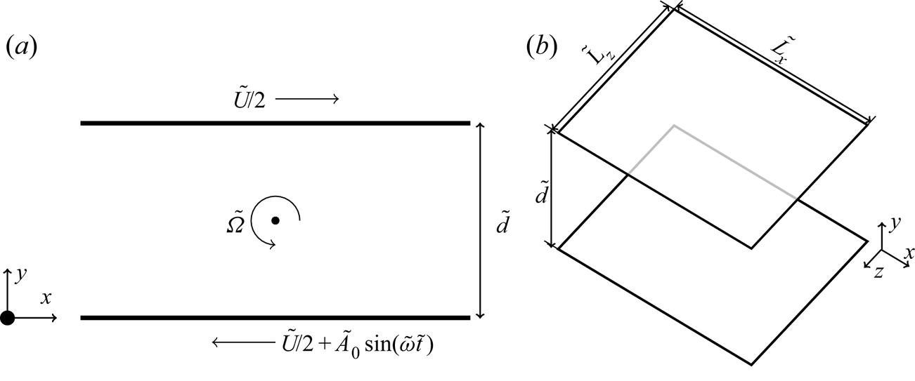
The top and bottom plates are no-slip, and prescribed to have equal and opposite streamwise velocities  $\pm (\tilde {U}/2)\boldsymbol {e}_x$, where
 $\boldsymbol {e}_i$ is the unit vector in the
 $i$-direction. In addition to this steady shear, a modulation is superimposed onto the bottom plate's velocity with a perturbation frequency
 $\tilde {\omega } = 2 {\rm \pi}/ \tilde {T}$ and magnitude
 $\tilde {A}_0$ such that the total velocity at the bottom plate is
 $-\tilde {U}/2+\tilde {A}_0\sin (\tilde {\omega }\tilde {t})$, with
 $\tilde {t}$ and
 $\tilde {T}$ the dimensional time and period, respectively.
The incompressible Navier–Stokes equations are made dimensionless using the gap width  $\tilde {d}$ and the plate velocity
 $\tilde {U}$. They read
 \begin{equation} \frac{\partial \boldsymbol{u}}{\partial t} + \boldsymbol{u}\boldsymbol{\cdot} \boldsymbol{\nabla} \boldsymbol{u} + R_\varOmega (\boldsymbol{e}_z \times \boldsymbol{u}) ={-}\boldsymbol{\nabla} p + Re_s^{{-}1}\,\nabla^2 \boldsymbol{u}, \end{equation}
which alongside the incompressibility condition defines the flow field,
 \begin{equation} \boldsymbol{\nabla} \boldsymbol{\cdot} \boldsymbol{u} = 0. \end{equation}
Here,  $\boldsymbol {u}$ is the non-dimensional velocity,
 $p$ is the non-dimensional pressure, and
 $t$ is the dimensionless time
 $t=\tilde {t}U/d$. Equation (2.1) contains two non-dimensional control parameters: a shear Reynolds number
 $Re_s=\tilde {U}\tilde {d}/\nu$, and the Coriolis parameter (sometimes known as the rotation number)
 $R_{\varOmega }=2 \tilde {\varOmega }\tilde {d}/\tilde {U}$, with
 $\tilde {\varOmega }$ the background spanwise rotation. Two more control parameters are provided by the modulated boundary condition: the non-dimensional modulation amplitude
 $\alpha =\tilde {A}_0/\tilde {U}$, and the non-dimensionalized modulation frequency, which is written as the Womersley number (
 $Wo$) defined as
 $\tilde {d} \sqrt {\tilde {\omega }/\nu }$ following Verschoof et al. (Reference Verschoof, te Nijenhuis, Huisman, Sun and Lohse2018). Using this, the dimensionless streamwise velocity boundary conditions become
 $\boldsymbol {u}=-\boldsymbol {e}_x/2$ at the top plate and
 \begin{equation} \boldsymbol{u}=\frac{1}{2}+\alpha\sin\left (\frac{t}{T} \right ) \boldsymbol{e}_x=\frac{1}{2}+\alpha\sin\left (\frac{Wo^2}{2{\rm \pi}\,Re_s}\,t \right) \boldsymbol{e}_x \end{equation}
at the bottom one, with  $T=2{\rm \pi} \,Re_s/Wo^2$ the non-dimensional period.
Periodic aspect ratios  $L_x=\tilde {L}_x/\tilde {d}=2{\rm \pi}$ and
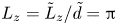 $L_z=\tilde {L}_z/\tilde {d}={\rm \pi}$ are used. The Reynolds number
 $Re_s$ is fixed at
 $3 \times 10^4$, resulting in a frictional Reynolds number
 $Re_\tau = u_\tau \tilde {U} \tilde {d}/(2\nu )= u_\tau Re_s/2 \approx 400$ for the non-rotating case, where
 $u_\tau$ is the non-dimensional shear velocity defined as
 $u_\tau = Re_s^{-1/2} \sqrt {\partial _y \langle u_x(y=0) \rangle _{A}}$, where
 $\langle \cdot \rangle _{A}$ denotes averaging with respect to time and to the streamwise and spanwise directions. For convenience, we also define a dimensionless frictional time unit
 $t_\tau =\tilde {t} u_\tau \tilde {U}/\tilde {d} = t u_\tau$, which will become useful later. We note that
 $t_\tau$ is a diagnostic time that does not appear in our equations, as
 $u_\tau$ is determined dynamically.
The rotation number  $R_{\varOmega }$ is varied in the range
 $[-0.1, 0.3]$, with positive values denoting anti-cyclonic rotation, such that the spanwise rotation vector is anti-parallel to the vorticity of base flow, whereas negative values signify cyclonic behaviour, i.e. the spanwise rotation is parallel to the vorticity vector of the base flow. The perturbation amplitude
 $\alpha$ is kept constant at
 $\alpha =0.1$ unless stated otherwise. The Womersley number
 $Wo$ is varied in the range
 $Wo\in [26,200]$, with selected cases at higher
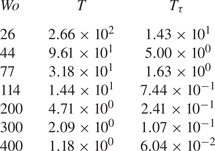
 $Wo$. Table 1 shows how these values of
 $Wo$ correspond to the different time scales in the flow, including the dimensionless forcing period in both dimensionless time units
 $t$ and
 $t_\tau$.
Summary of Womersley numbers used for all simulations, and their corresponding dimensionless forcing period  $T=\tilde {T}U/d$. We also include the forcing period in dimensionless frictional units
 $T_\tau$ defined as
 $T_\tau =(\tilde {T} u_\tau U)/(d/2)=2Tu_\tau$ to show how
 $T$ relates to the frictional time scales in the flow.
Equations (2.1) and (2.2) are discretized using finite differences: second-order accurate energy conserving in space, third-order accurate in time using Runge–Kutta for the explicit terms. The viscous term is discretized in the wall-normal direction using a second-order Crank–Nicolson scheme. The discretized equations are solved using the parallel FORTRAN-based code AFiD (www.afid.eu). This code has been used in previous studies to study turbulent Rayleigh–Bénard convection and TCF (Van Der Poel et al. Reference Van Der Poel, Ostilla-Mónico, Donners and Verzicco2015), and has been validated thoroughly. Details of the code algorithms are documented in Verzicco & Orlandi (Reference Verzicco and Orlandi1996) and Van Der Poel et al. (Reference Van Der Poel, Ostilla-Mónico, Donners and Verzicco2015). Spatial resolution of the simulations are selected as  $N_x \times N_y \times N_z = 512\times 384\times 512$ in the streamwise, wall-normal and spanwise directions, respectively. The points are distributed uniformly in the streamwise and spanwise directions, while for the wall-normal direction they are clustered near the walls using a clipped Chebyshev distribution. This gives us an effective resolution in viscous wall units of
 $\Delta x^+=9.8$,
 $\Delta z^+=4.9$ and
 $\Delta y^+ \in (0.3,3.0)$. This resolution is chosen in accordance with the spatial resolution selected for
 $Re_s=3.61 \times 10^4$ in the study of turbulent Taylor rolls in Sacco et al. (Reference Sacco, Verzicco and Ostilla-Mónico2019). For a series of selected cases, we double
 $L_x=4{\rm \pi}$ and
 $L_z=2{\rm \pi}$ to check the dependence of the statistics on the box size. For these cases, we also double the resolutions in the
 $x$- and
 $z$-directions to keep the same base grid spacing.
A variable time-stepping scheme is defined such that the maximum Courant–Friedrichs– Lewy condition does not exceed 1.2. To exclude the start-up transients, the first 200 time units are discarded before starting to evaluate the statistics. The duration of the simulation to evaluate turbulence statistics is 10 periods from the end of the transient (except for  $Wo=26$, for which it is 5 due to long run times) for a given
 $Wo$ number, or 1000 simulation time units, whichever is larger.
Temporal convergence is also checked by monitoring that the  $y$-dependence of the computed non-dimensional momentum flux
 \begin{equation} J^\omega = \langle u_x u_y \rangle_{A} - Re_s^{{-}1}\,\frac{\partial \langle u_x \rangle_{A}}{\partial y} \end{equation}
does not exceed 1 %. While  $J^\omega$ is independent of
 $y$ for sufficiently long averaging times, in our simulations it will show a
 $y$-dependence due to finite averaging times. Therefore, quantifying the
 $y$-dependence of
 $J^\omega$ is a way to assess the errors made due to finite statistics. We note that performing this check includes checking that the shears at both walls are equal to within
 $1\,\%$, as the shear at the walls is simply
 $J^\omega$.
3. Results for non-rotating plane Couette flow
The first case that we analyse is PCF without rotation, i.e.  $R_\varOmega =0$. Non-rotating PCF contains large-scale structures that extend significantly in the streamwise direction (Tsukahara, Kawamura & Shingai Reference Tsukahara, Kawamura and Shingai2006). However, these structures do not dominate the transport of momentum in the same way that the Taylor rolls present for
 $R_\varOmega =0.1$ (Brauckmann et al. Reference Brauckmann, Salewski and Eckhardt2016; Sacco et al. Reference Sacco, Verzicco and Ostilla-Mónico2019; Sacco, Ostilla-Mónico & Verzicco Reference Sacco, Ostilla-Mónico and Verzicco2020). Instead, momentum is transferred through a hierarchy of eddies that spans many length- and time-scales (Townsend Reference Townsend1980), so in principle we do not expect that there are natural time scales in the flow with which the modulation could couple to produce resonances.
We look first at the volumetrically averaged instantaneous dissipation  $\varepsilon$, which is a quantity of interest in studies of modulated turbulence. We note that the temporal average of
 $\varepsilon$ is equal to the shear force at the plates (modulo scaling factors) due to the exact balances of energy: in the statistically stationary state, on average, energy input through the walls must be balanced out by the viscous dissipation.
To represent this, we follow Brauckmann et al. (Reference Brauckmann, Salewski and Eckhardt2016) and Eckhardt, Doering & Whitehead (Reference Eckhardt, Doering and Whitehead2020) to define two Nusselt numbers. First, we define a force Nusselt number  $Nu$ as
 $Nu=J^\omega /J^\omega _{lam}$, where
 $J^\omega _{lam}$ is the momentum current for the laminar state. By definition,
 $Nu=1$ in the purely streamwise flow. Second, we define a Nusselt number
 $Nu_\varepsilon$ based on the instantaneous viscous dissipation,
 $Nu_\varepsilon = \varepsilon /\varepsilon _{lam}$. We note that due to the exact balances, while the instantaneous value of
 $Nu_\varepsilon$ will be distinct from instantaneous force Nusselt number
 $Nu$, the time-averaged value of
 $Nu_\varepsilon$ will equal
 $Nu$.
In figure 2(a), we show the instantaneous values of  $Nu_\varepsilon$ for two different values of
 $Wo$ (44 and 200) and for the unmodulated flow. Here, time is non-dimensionalized using the frictional time scale. In figure 2(b), we use the modulation period
 $T$ to non-dimensionalize time, and show only the instantaneous values of
 $Nu_\varepsilon$ for the modulated cases. This choice re-scales the horizontal axis differently for both lines, and reveals how there are two clear time scales in the flow, one given by the modulated forcing from the wall, of order
 ${O}(T)$, and one given by the turbulent flow itself, of order
 ${O}(t_\tau )$. The fluctuations due to natural turbulence appear to be much smaller than those introduced by modulation (figure 2a), which are of the order of 20–30 % around the mean value of
 $Nu_\varepsilon$ even when the wall-modulation amplitude is only 10 % of the average wall velocity. We also note that the fluctuation size does not appear to change appreciably with the modulation frequency, unlike what was observed in Jin & Xia (Reference Jin and Xia2008), a fact to which we will return later.
(a) Temporal evolution of the averaged dissipation, non-dimensionalized as a Nusselt number ( $Nu_\varepsilon$) for unmodulated flow (black),
 $Wo=44$ (blue) and
 $Wo=200$ (red). (b) As in (a), with the time units re-scaled using the period of the forcing. (c) Temporally averaged
 $Nu_{\varepsilon}$ against
 $Wo$ for the non-rotating case. The blue points denote the baseline periodic aspect ratios of
 $L_x=2{\rm \pi}$ and
 $L_z={\rm \pi}$, while the orange data points are simulations to check the effect of domain size with
 $L_x=4{\rm \pi}$ and
 $L_z=2{\rm \pi}$.
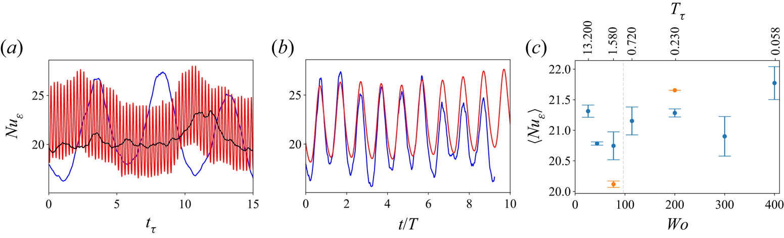
To elucidate how the average value of dissipation (and wall shear) depends on the parameters of the unsteady forcing, we show the temporally averaged values of  $Nu_\varepsilon$ in figure 2(c). We cannot observe any definite patterns in the resulting values for total dissipation; they deviate from the value
 $\langle Nu_\varepsilon \rangle = 20.6\pm 0.2$ obtained with no modulation, but this baseline value is generally contained within the error bars of the simulation. This provides a first indication that the modulation does not couple significantly with any existing structures in the flow, even for
 $Wo=77$ and
 $Wo=114$, when the modulation roughly matches the time scale of the flow, i.e.
 $T_\tau \approx 1$. To assess the possible effects of box-size dependence on these results, we simulated two additional cases at twice the domain size for
 $Wo=77$ and
 $Wo=200$, shown with orange markers in figure 2(c). These values of
 $Nu$ also show some dispersion around the baseline value. We note that the
 $Wo=77$ case is
 $4\,\%$ below the previous value, which would result in a smaller friction at the walls and is consistent with similar studies of PCF (Tsukahara et al. Reference Tsukahara, Kawamura and Shingai2006). However, this is not seen for
 $Wo=200$, where the resulting
 $Nu$ is instead larger. We conclude by stating that the error introduced by the small domain size is comparable to or larger than any variation due to
 $Wo$, which means that we cannot make any definite statements on the
 $Nu(Wo)$ dependence; even if following Jin & Xia (Reference Jin and Xia2008), we do not expect there to be an effect.
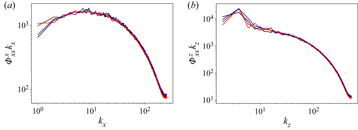
We first check the effect of modulation on the flow structures by showing the streamwise and spanwise spectra of the streamwise velocity in figure 3. The periodic modulation does not introduce significant modifications of the energy spectra at the mid-gap. Only a small degree of variation between the cases, especially at the low wavenumber end, can be seen, and among these there is no discernible pattern of behaviour as the curves are not ordered by  $Wo$. This is similar to what was seen for
 $Nu$, where no discernible pattern could be seen as
 $Wo$ was changed. We also note that for the streamwise spectra
 $\varPhi _{xx}^x$, the unmodulated case is closest of all to the lowest
 $Wo$ curve (
 $Wo=44$) – something that is unexpected. Due to the absence of obvious patterns, we may attribute these differences to insufficient temporal convergence of the statistics shown in the graphs.
Time-averaged pre-multiplied (a) streamwise and (b) spanwise spectra of the streamwise velocity at the mid-gap ( $y=0.5$) for non-rotating PCF. The colours indicate:
 $Wo=44$, black;
 $Wo=77$, red-brown;
 $Wo=200$, bright red; unmodulated, dark blue.
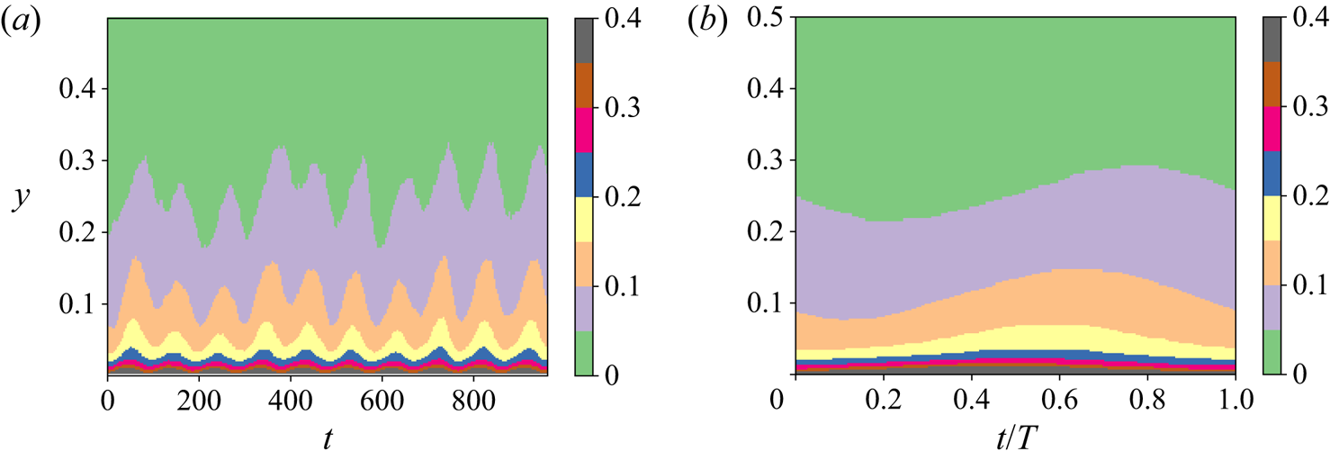
To understand how the modulation is transferred through the flow, we turn towards the streamwise velocity field itself. To isolate the effect of the modulation from the turbulent background fluctuations, we first average the field in the spanwise and streamwise directions. A space–time visualization of the result in shown in figure 4(a). The modulation imposed by the unsteady boundary condition can be seen clearly. Due to the turbulent fluctuations, the average velocities are not periodic. To separate the effect introduced by the periodic motion of the wall, we conduct a phase average over several of the periods simulated. This reduces the temporal domain to  $0\leq t/T < 1$, resulting in a phase-averaged velocity field that we denote as
 $\bar {u}(y,t/T)$. We show a space–time visualization of
 $\bar {u}$ in figure 4(b), where we can now see clearly how the modulation wave travels from the wall into the rest of the fluid, observing that as the distance from the wall increases, the phase lag becomes larger.
Space–time pseudo-colour plots of the averaged streamwise velocity up to the mid-gap for  $Wo=44$, non-rotating case. (a) Instantaneous streamwise- and spanwise-averaged velocity. (b) Spanwise-, streamwise- and phase-averaged velocity.
We can decompose  $\bar {u}$ as
 \begin{equation} \bar{u}(y,t/T) = \bar{u}_0(y) + f(y,t/T), \end{equation}
where  $\bar {u}_0$ is the temporally averaged velocity, and
 $f(y,t/T)$ denotes the periodic effect introduced by the modulation. This paper will focus on the behaviour of
 $f(y,t/T)$, but before we do so, we wish to mention that the behaviour of
 $\bar {u}_0$ is not very different from that seen in unmodulated rotating PCF. While the basic symmetry is broken, it is restored in a temporally-averaged sense, and as a consequence, when we examine the behaviour of the average streamwise velocity, for example, we cannot observe an asymmetry between the modulated and unmodulated walls.
Returning to  $f$, there is no a priori reason to think that it cannot contain any harmonics of the fundamental modulation of period
 $T$, i.e.
 $T/2$,
 $T/3$, etc. However, the visualization shown in figure 4(b) indicates that the dominant temporal scale is that associated with the modulation, and not higher harmonics. This is confirmed further by Fourier analysis, which shows that the second harmonic has an amplitude that is a factor 10–300 times smaller than the first fundamental, depending on the distance to the wall.
Therefore, we use the ansatz that  $f$ has the following functional dependence:
 \begin{equation} f(y,t/T) = A_u(y) \sin[2{\rm \pi} t/T + \phi_{d}(y)], \end{equation}
where  $A_u$ is the amplitude response, and
 $\phi _{d}$ the phase lag, both of which are dependent on the distance to the wall. To determine the values of these quantities, we use two methods. The first is to simply take a Fourier transform of
 $f$, and determine
 $\phi _{d}$ and
 $A_u$ from the results of this transform. We truncate
 $\phi _d$ when the amplitude of the Fourier mode is smaller than
 $10^{-3}$, for reasons that will become apparent below. For comparison purposes, we also follow Verschoof et al. (Reference Verschoof, te Nijenhuis, Huisman, Sun and Lohse2018), and determine the phase delay using the peak of the cross-correlation between the wall velocity and
 $f$. We show the results obtained from both methods in figures 5(a,b) for values of
 $Wo$ in the
 $(26,200)$ range. We have also added dashed lines that represent the exact solution for Stokes’ oscillating laminar boundary layer,
 $\phi _{d}=(y\,Wo)/\sqrt {2}$.
(a,b) Phase delay  $\phi _{d}$ against wall distance for the non-rotating cases measured through FFT (a) and using the cross-correlation method of Verschoof et al. (Reference Verschoof, te Nijenhuis, Huisman, Sun and Lohse2018) (b). (c) Perturbation time lag with respect to wall against wall distance for non-rotating cases. (d) Amplitude response
 $A_{u}$ measured through the FFT method against wall distance for the non-rotating cases. The lines represent
 $Wo=26$,
 $44$,
 $77$,
 $114$,
 $200$ from light red to dark red. Dashed lines are the theoretical results from Stokes’ problem.
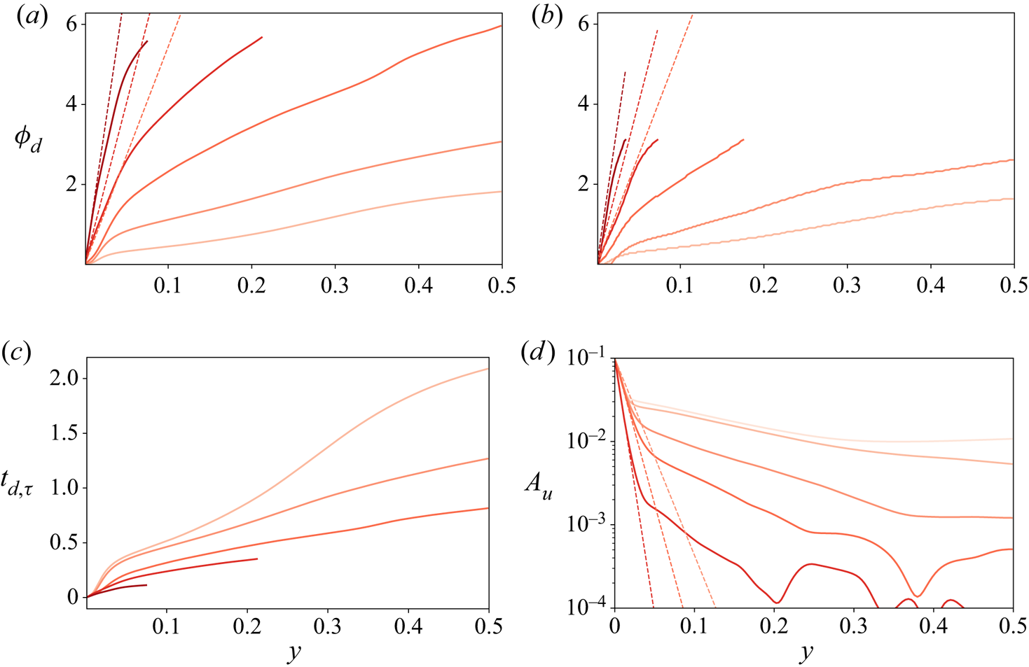
We first notice that the phase delay results for the cross-correlation are limited to the range  $[0,{\rm \pi} )$, while those obtained from the Fourier transform have a larger range of
 $\phi$ that is limited only by truncation. The results are also qualitatively similar to each other, with a few minor differences. In the cross-correlation method, the phase delay is effectively zero for the lowest
 $Wo$ very close to the wall, and is slightly smaller than the one obtained through the Fourier transform. This method also shows some ‘graininess’ due to the numerical inadequacies of using the maximum operator. Hence we use the Fourier transform for measuring
 $A_u$ and
 $\phi _{d}$, as the trend is more distinct, even if it is evident that the cross-correlation calculation used in Verschoof et al. (Reference Verschoof, te Nijenhuis, Huisman, Sun and Lohse2018) also gives reasonable results.
Turning to the results themselves, we can observe that there are two distinct regions where the phase and the wall distance are related in an approximately linear manner, albeit with different slopes. A linear relationship between phase and wall distance can be understood as information from the modulation propagating into the flow with a constant speed, with the phase delay acting as a proxy for time ( $\phi _d\sim t/T$). In this way, a steeper slope
 $m$ in the
 $\phi _d=my$ line signals a slower travel velocity. The lines change from one slope to another at
 $y\approx 0.05$, which corresponds to
 $y^+\approx 40$, i.e. the buffer subregion of the boundary layer. Hence the region
 $y \le 0.05$ corresponds approximately to the viscid subregion where the modulation travels slower, mainly through viscosity. The other flow region (
 $y \ge 0.05$) corresponds to zones in the buffer layer and beyond. It has a shallower slope, which means that the modulation travels faster, as it is essentially transported by turbulent fluctuations.
In the viscous region ( $y\le 0.05$), the slopes obtained are shallower than the purely viscid solutions (denoted as dashed lines), so other mechanisms that accelerate the transport are at play. We also highlight that the distance between the purely viscous solution and the actual solution decreases as the frequency increases, meaning that these corrections become less important. We can also observe that the phase delay is larger with increasing
 $Wo$ at a given wall distance. This does not mean that the perturbation itself travels slower. Instead, it means that increasing the frequency of the perturbation does not increase the travel speed of the perturbation by an amount sufficient to make the phase delay constant at a given distance. To emphasize this point, we show the actual delay time in frictional time units
 $t_{d,\tau }$ against wall distance for all values of
 $Wo$ in figure 5(c). Again, we can see two regions with different behaviours: the viscous subregion at
 $y\le 0.05$, and the turbulent region for
 $y>0.05$. In the near-wall region, if
 $Wo$ is large (dark curves), then the perturbation travel speed is fast and depends strongly on
 $Wo$. If
 $Wo$ is small (light curves), then the travel speed of the perturbation is slower and the two curves seem to almost lie on top of each other for small values of
 $y<0.03$. This is consonant with the fact that high-
 $Wo$ curves follow the Stokes solution better than their low-
 $Wo$ counterparts in the viscid region.
We can observe similar behaviour in the turbulent region, where all lines reported (except for  $Wo=26$) have a similar slope, indicating that the actual velocity at which the perturbation travels is approximately
 $Wo$-independent in the bulk. The transition between high-
 $Wo$ and low-
 $Wo$ behaviour is not easy to delimit, as some curves show different characteristic behaviour depending on the wall distance. For
 $Wo=26$, due to low travel speed, we do not expect a simple picture. Once the delay time grows beyond
 $t_\tau =1$, the information from more than one modulated cycle will be affecting the flow. Finally, we notice that for
 $Wo=77$, the phase delay is approximately
 $2{\rm \pi}$ at the centre; in contrast, for
 $Wo=44$, it takes approximately
 $t_\tau =1$ time units for the perturbation to reach the centre. This confirms the fact that we are forcing close to the natural time scale of the flow, as suggested by table 1. However, we do not see any sort of resonant behaviour in the dissipation – neither for
 $Wo=77$ nor for
 $Wo=44$.
We now turn to the amplitude response  $A_u$. We show here only results obtained through the Fourier transform method, which presents much smaller oscillations than applying the method used in Verschoof et al. (Reference Verschoof, te Nijenhuis, Huisman, Sun and Lohse2018) on our data. In figure 5(d), we show
 $A_u$ as a function of wall distance for the same five
 $Wo$ values. We also include the solutions of Stokes’ second problem for the three largest values of
 $Wo$, which are given by
 $A_u=\exp (-\sqrt {2}\,Wo\,y)$. These are represented as straight lines in our semi-logarithmic plot. The same two regions as in the phase plot can be seen: there is an inner viscid region where the perturbation amplitude decays rapidly, and which tracks the viscous solution closely. There is also a turbulent region where the perturbation decay is slower. And again, the transition between both regions happens at
 $y\approx 0.05$. When
 $y>0.05$, the perturbations are transported through turbulence, which can be understood as an effective increase of the viscosity, which in turn facilitates the propagation of the perturbation, resulting effectively in a slower decay rate. For the case
 $Wo=26$, we can observe a third region that starts at around
 $y=0.3$, where the slope further decreases to the point that the amplitude is almost constant. The origin of this third region is unclear, as similar changes did not appear clearly in the phase delay but were present when looking at the delay time. In principle, we can rule out averaging errors due to the rather large magnitude of
 $A_u$. Finite-averaging and other numerical errors are expressed in the manner seen for the two highest values of
 $Wo$: through oscillations that start to dominate only once
 $A_u<10^{-3}$, i.e. as the perturbation amplitude has decreased by
 ${O}(10^2)$. A possible source of this could be that in this region, the delay time from the wall exceeds a modulation cycle, causing more complicated interactions.
To allow a more direct comparison with the results from Verschoof et al. (Reference Verschoof, te Nijenhuis, Huisman, Sun and Lohse2018), we plot the amplitude and phase lag as functions of  $Wo$ for different
 $y$-locations in figures 6(a,b). Unlike the corresponding figures in Verschoof et al. (Reference Verschoof, te Nijenhuis, Huisman, Sun and Lohse2018), these plots show that the amplitude and phase delay of the perturbation are strong functions of the distance to the wall. There are two main possible sources for this discrepancy. First, we show values of
 $y$ that are much closer to the wall, down to
 $y=0.01$, while Verschoof et al. (Reference Verschoof, te Nijenhuis, Huisman, Sun and Lohse2018) use distances that correspond to the range
 $0.2< y<0.8$. Second, not only the Reynolds number is different, but also the rotation rate. TCF with a pure inner cylinder rotation corresponds to a rotation number
 $R_\varOmega =1-\eta$, with
 $\eta$ being the radius ratio
 $\eta = r_i/r_o$, where
 $r_i$ is the inner cylinder radius, and
 $r_o$ is the outer cylinder radius. This means that the effective value of
 $R_\varOmega$ in the experiments is
 $R_\varOmega =0.286$, as the radius ratio is
 $\eta =0.714$. We will visit that value of
 $R_\varOmega$ in a later section, and show that the effective solid-body rotation is indeed the main source of our discrepancy.
(a) Amplitude response ( $A_{u}$) against
 $Wo$ for non-rotating cases. The black dashed line shows the scaling
 $A_u \sim Wo^{-2}$, and the inset shows the compensated amplitude
 $A_uWo^2$ against
 $Wo$ plot to emphasize the scaling. (b) Phase delay (
 $\phi _{d}$) using FFT against
 $Wo$ for non-rotating cases. Cases shown are
 $y=0.01, 0.05, 0.1, 0.5$ from light blue to dark blue. The grey vertical dashed lines mark
 $T_\tau=1$.

To summarize, there are two distinct regimes for  $A_u(Wo)$. At low
 $Wo$, the amplitude is not a strong function of
 $Wo$. This region is especially pronounced for the data at
 $y=0.01$ for
 $Wo<100$. At high
 $Wo$, the amplitude decays rapidly as
 $Wo$ is increased. This decrease matches the prediction in von der Heydt et al. (Reference von der Heydt, Grossmann and Lohse2003a): for high
 $Wo$, the amplitude should behave like
 $A_u\sim T$. This is shown in figure 6(a) as the dashed line
 $A_u\sim Wo^{-2}$ and emphasized in a compensated subplot. This theoretical scaling matches the data reasonably well. As we move away from the wall, the transition to the
 $A_u\sim Wo^{-2}$ dependence happens at lower values of
 $Wo$. We can attribute this to the flow finding it harder to adjust to the perturbation as the distance to the wall increases. This two-region behaviour is also seen for the phase lag, shown in figure 6(b), even if no clear power-law behaviour can be discerned or is available from the theoretical derivations in von der Heydt et al. (Reference von der Heydt, Grossmann and Lohse2003a).
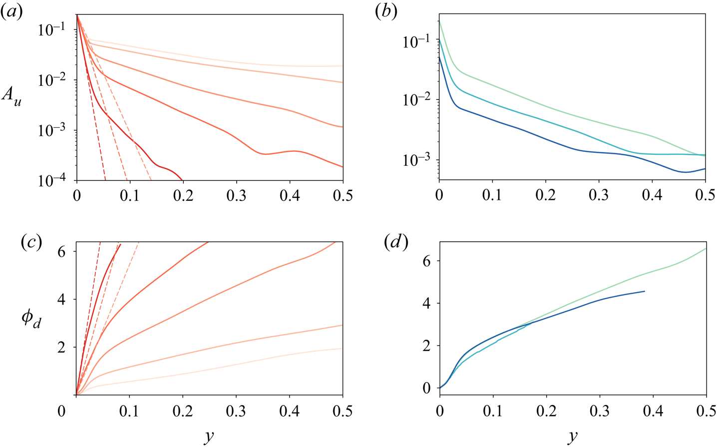
For completeness, we checked the effect of the amplitude  $\alpha$ on the results by running all the cases shown above for
 $\alpha =0.05$ and
 $\alpha =0.2$. A short summary of the results is presented in figure 7. In figures 7(a,c), we show the amplitude response and the phase delay against wall distance for all values of
 $Wo$ and
 $\alpha =0.2$. We can see the same qualitative phenomena that we saw appear for
 $\alpha =0.1$, which we have discussed previously. We do not show these results for
 $\alpha =0.05$ as they show the same patterns, but the numerical averaging errors appear for smaller values of
 $y$ due to the smaller amplitude of the perturbation. In figures 7(b,d), we show
 $A_u$ and
 $\phi _d$ against
 $y$ for different values of
 $\alpha$ and the same
 $Wo$. We can see clearly that the amplitude response of the system is simply offset by a factor, while the phase response is approximately independent of
 $\alpha$ except for some small discrepancies that we attribute to insufficient statistics.
(a) Amplitude response ( $A_{u}$) against wall distance for
 $\alpha =0.2$ and varying
 $Wo$. Colours are the same as in figure 5. (b) Amplitude response against wall distance for
 $Wo=77$ and
 $\alpha =0.05$ (dark) ,
 $\alpha =0.1$ (mid) and
 $\alpha =0.2$ (light). (c,d) As in (a,b) for phase delay (
 $\phi _d$).
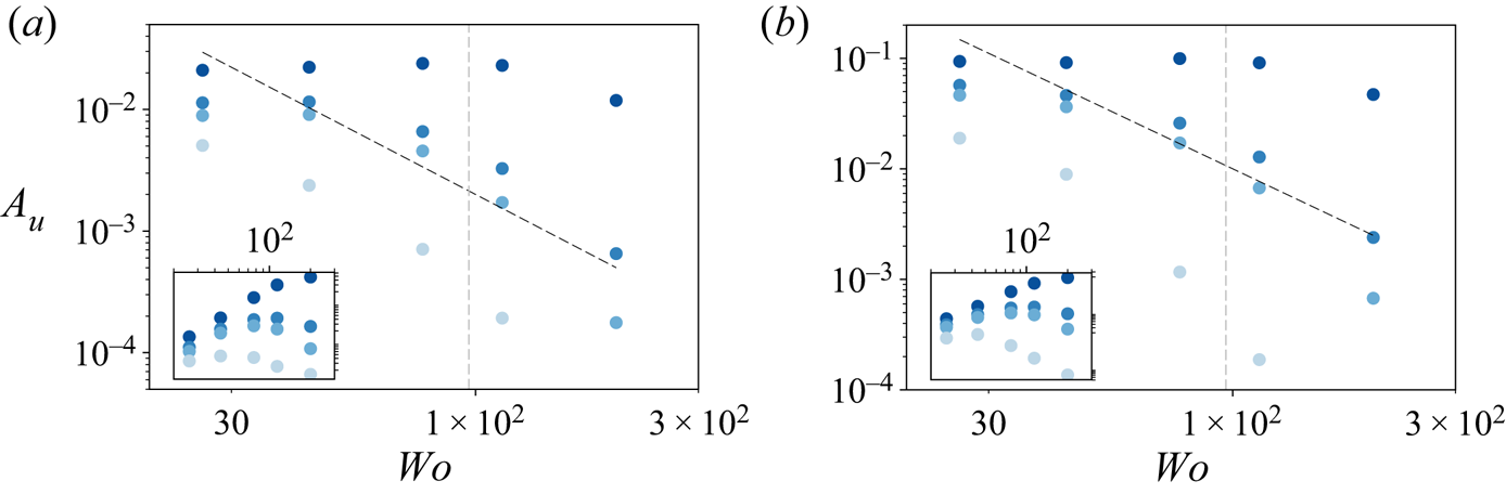
Finally, in figure 8, we show an analogue to figure 6 but for the two other values of  $\alpha$ simulated (0.05 and 0.2). It shows the same
 $A_u\sim Wo^{-2}$ behaviour in the high-
 $Wo$ regime. This gives us confidence in the fact that for small values,
 $\alpha$ is a physically unimportant parameter that is relevant only when considering the effect of numerical averaging errors. We can expect that for
 $\alpha \sim {O}(1)$, significant effects of the amplitude modulation will begin to be seen in
 $Nu$, similar to those in Yang et al. (Reference Yang, Chong, Wang, Verzicco, Shishkina and Lohse2020).
Amplitude response ( $A_{u}$) against
 $Wo$ for non-rotating cases and (a)
 $\alpha =0.05$, (b)
 $\alpha =0.2$. For each plot, the black dashed line shows the scaling
 $A_u \sim Wo^{-2}$, and the inset shows a plot of the compensated amplitude
 $A_u\,Wo^2$ against
 $Wo$ to emphasize the scaling. The grey vertical dashed lines mark
 $T_\tau=1$.
4. Results for rotating plane Couette flow
4.1. Modulation and Taylor rolls
Adding solid-body rotation causes a drastic change in the flow behaviour and modifies the underlying statistics such as dissipation and mean velocity (Brauckmann et al. Reference Brauckmann, Salewski and Eckhardt2016). As mentioned earlier, it also triggers the formation of large-scale pinned structures known as Taylor rolls, which are responsible primarily for the transport of shear. These rolls are in close analogue with the large-scale structures in Rayleigh–Bénard flow that dominate heat transfer. Further, such large-scale structures couple to modulation introduced through the driving boundary (oscillating wall) (Jin & Xia Reference Jin and Xia2008; Yang et al. Reference Yang, Chong, Wang, Verzicco, Shishkina and Lohse2020).
We start our discussion with  $R_\varOmega =0.1$, which is the value of
 $R_\varOmega$ for which the rolls are most energetic (Sacco et al. Reference Sacco, Verzicco and Ostilla-Mónico2019). Therefore, we can expect this to be the most favourable case to observe resonant coupling between the modulation and the existing structures in the flow, as the structures have very well-defined natural length and time scales. We first show the instantaneous
 $Nu_\varepsilon (t)$ in figures 9(a,b) for
 $R_\varOmega =0.1$ and
 $Wo=44$,
 $200$, and unmodulated flow (black line in figure 9a). The temporal fluctuations due to the inherent turbulence of the flow are even smaller than for the case with no rotation. The modulation introduces fluctuations in
 $Nu_\varepsilon (t)$ that are of the order of 20–30 % of the mean value of
 $Nu_\varepsilon$, i.e. the same order of magnitude as the values observed previously. We can also observe that the fluctuations in
 $Nu_\varepsilon$ are larger for smaller values of
 $Wo$, similar to what was observed in Jin & Xia (Reference Jin and Xia2008). We propose an explanation for this below.
(a) Temporal evolution of the averaged dissipation, non-dimensionalized as a Nusselt number ( $Nu_\varepsilon$) for unmodulated flow (black),
 $Wo=44$ (blue) and
 $Wo=200$ (red), with
 $R_\varOmega =0.1$. (b) Same as in (a), with the time units re-scaled using the period of the forcing. (c) Temporally averaged
 $Nu_\varepsilon$ against
 $Wo$ for
 $R_\varOmega =0.1$. Blue points denote the baseline periodic aspect ratios of
 $L_x=2{\rm \pi}$ and
 $L_z={\rm \pi}$ with single-roll pairs, while green points denote the same domain for two-roll pairs. The orange data points are simulations to check the effect of domain size with
 $L_x=4{\rm \pi}$ and
 $L_z=2{\rm \pi}$, and two-roll pairs (with the same roll size as the baseline).
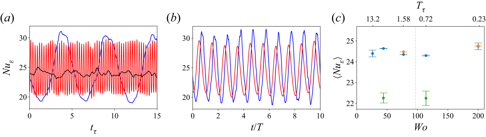
Similar to the non-rotating case, the mean value around which all curves fluctuate appears to be the same. To further quantify this, in figure 9(c) we show the time-averaged values of  $Nu_\varepsilon$ as a function of
 $Wo$. As was seen for the non-rotating case, no strong dependence of
 $Nu_\varepsilon$ on
 $Wo$ is observed. This hints at the fact that no significant resonances happen between the modulated forcing and the existing structure. These results are consistent with those obtained in Jin & Xia (Reference Jin and Xia2008) for sinusoidally modulated RBC, where no enhancement was observed in the time-averaged values of heat transport. We also confirm that the dependence of
 $Nu$ on domain size is much smaller for the RPCF.
We note that in all cases discussed here, we are analysing simulations with a single-roll pair, such that the roll wavelength is  $\lambda _{TR}=L_z={\rm \pi}$. The possibility for other roll states with different wavelengths to arise and persist in rotating PCF and TCF is well-documented (Ostilla-Mónico, Lohse & Verzicco Reference Ostilla-Mónico, Lohse and Verzicco2016a; Xia et al. Reference Xia, Shi, Cai, Wan and Chen2018). The number of rolls in a simulation is very dependent on the initial conditions, and through our choices, we obtain simulations having a single-roll pair state. The adding of modulation at
 $\alpha =0.1$ is not strong enough to change the roll state in our selected domain size, and we did not see any effect of the modulation on these rolls. There still was a single-roll pair in the averaged fields after turning the modulation on. By manipulating the initial conditions, we were able to generate states with two pairs of rolls for
 $Wo=44$ and
 $Wo=114$, such that the roll wavelength was now
 $\lambda _{TR}=L_x/2={\rm \pi} /2$. These show the same properties in the Nusselt number discussed above: larger oscillations with small
 $Wo$, and small oscillations with large
 $Wo$. However, the average Nusselt number value was lower, consistent with what was discussed in Ostilla-Mónico et al. (Reference Ostilla-Mónico, Van Der Poel, Verzicco, Grossmann and Lohse2014), where it was observed that for TCF at similar values of
 $Re_s$, small rolls would produce lower values of the torque.
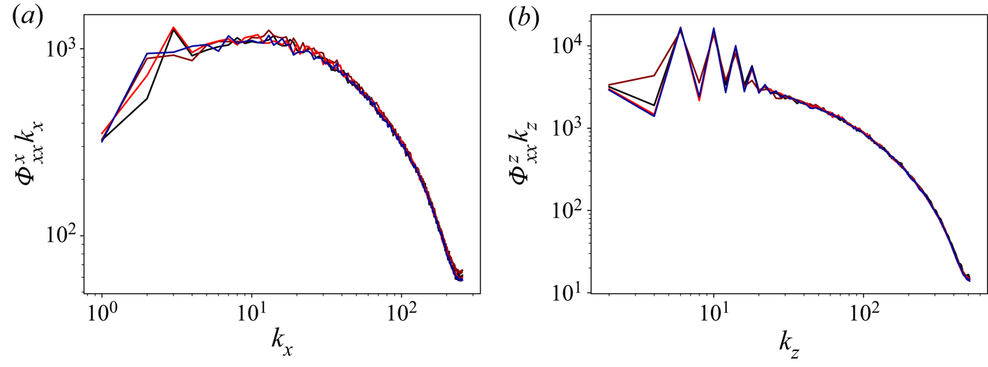
Further proof of the robustness of the rolls to modulation is provided by the velocity spectra. We show the energy spectrum of the streamwise velocity in figure 10. The ‘sawtooth’ pattern characteristic of Taylor rolls (cf. Ostilla-Mónico et al. Reference Ostilla-Mónico, Verzicco, Grossmann and Lohse2016b) can be appreciated for the spanwise spectra  $\varPhi _{xx}^z$. Some modification of the pattern is observed for
 $Wo=77$, which is the value of
 $Wo$ that more closely matches the natural time scales of the flow, and is the one that we expect to produce resonant effects. However, this modification does not correspond to a significant change in the value of
 $\langle Nu_\varepsilon \rangle$. Instead, we postulate that the modes that are normally dampened or eliminated by the Taylor rolls, i.e. the second, fourth and other even fundamentals, are more energetic than for the unmodulated values. However, because the first fundamental mode remains unaffected, which corresponds to the Taylor roll and hence transports the most shear, the resulting transport of shear is almost unaffected.
Time-averaged pre-multiplied (a) streamwise and (b) spanwise spectra of the streamwise velocity at the mid-gap ( $y=0.5$) for RPCF with
 $R_\varOmega =0.1$. The colours indicate:
 $Wo=44$, black;
 $Wo=77$, red-brown;
 $Wo=200$, bright red; unmodulated, dark blue.
Following the discussion in Jin & Xia (Reference Jin and Xia2008), it could be that sinusoidal modulations are too smooth to cause a resonance sufficient to increase the strength of the roll and hence change  $\langle Nu_\varepsilon \rangle$. We can justify this by looking at the energy of the Taylor roll. Following Sacco et al. (Reference Sacco, Verzicco and Ostilla-Mónico2019), we measure this energy as the energy
 $E_{01}$ of the first
 $z$-fundamental (i.e.
 $k_x=0$,
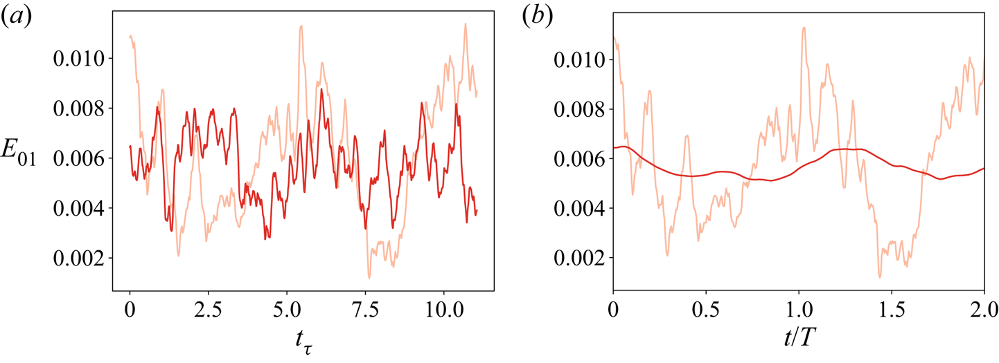
 $k_z=2$) of the wall-normal velocity at the mid-gap. In figure 11, we show the temporal behaviour of this quantity. For
 $Wo=200$, the inertia of the roll is large enough to absorb the forcing modulation. Conversely, for
 $Wo=44$, the time scale of the modulation becomes larger than
 $t_\tau = 1$. The roll's inertia is insufficient to absorb this slow modulation, and its signature appears as a larger fluctuations in
 $E_{01}$. This explains the larger fluctuations observed in
 $Nu(t)$ for small values of
 $Wo$ at
 $R_\varOmega$.
Temporal evolution of the energy of the fundamental Fourier mode associated with the Taylor roll in (a) flow and (b) forcing time units for  $R_\varOmega =0.1$. The light red lines indicate
 $Wo=44$; the dark red lines indicate
 $Wo=200$.
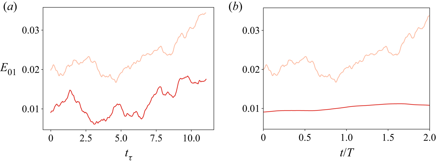
Moreover, the lack of large-scale shear-transporting structures at  $R_\varOmega =0$ means that we do not see an increased fluctuation level in figure 2. We can justify this further by looking at
 $E_{01}$ for the non-rotating case. We show the time evolution of this quantity in figure 12. We can see clearly that there is no obvious correlation between forcing and
 $E_{01}$, and the energy of the mode changes in time with no discernable pattern. This is further proof that while the modulated driving can affect large-scale structures, sinusoidal driving cannot achieve transport-enhancing resonances.
Temporal evolution of the energy of the fundamental Fourier mode associated with the Taylor roll in (a) flow and (b) forcing time units for non-rotating PCF. The light red lines indicate  $Wo=44$; the dark red lines indicate
 $Wo=200$.
Unfortunately, the presence of the roll prevents us from examining the way the modulated energy propagates into the flow, as the introduced spanwise dependence of average quantities makes replicating the earlier analysis of § 3 impossible. The decomposition introduced to calculate  $f$ as in (3.1) produces large artefacts that we will discuss later, in context with the results from other values of
 $R_\varOmega$.
4.2. Modulation and mean rotation
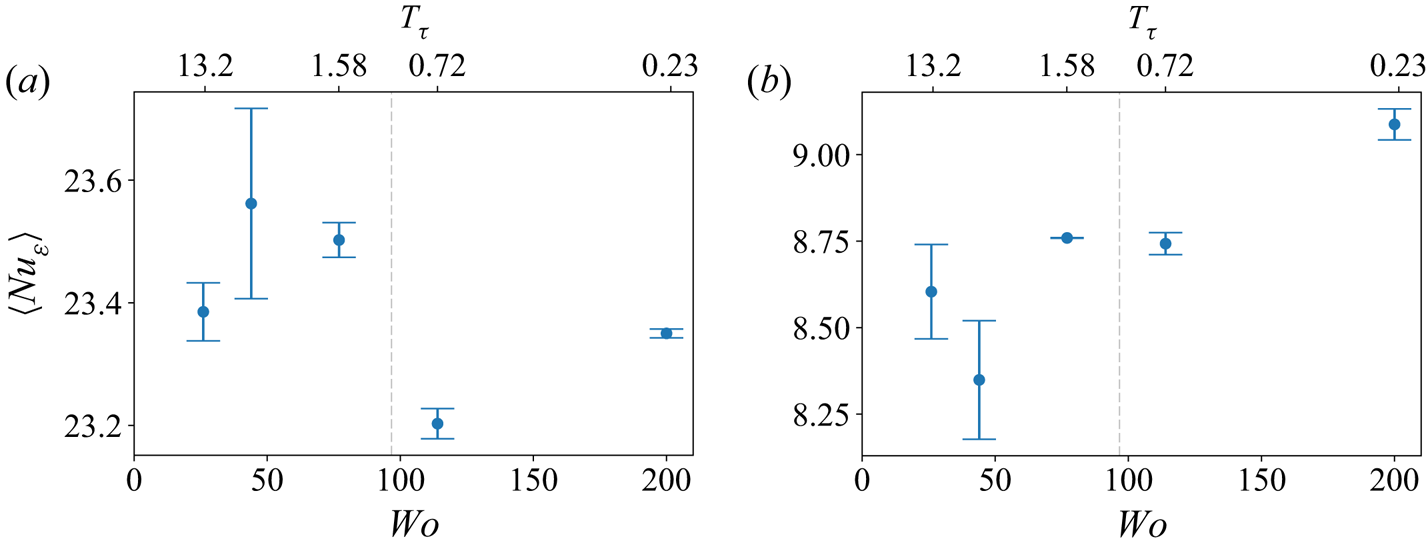
We start by analysing the effect of the remaining values of  $R_\varOmega$ on the behaviour of the shear transport and the dissipation. In figure 13, we show the time-averaged
 $Nu_\varepsilon$ against
 $Wo$ for the two remaining values of
 $R_\varOmega$ studied. As for the previous cases, no significant effect of
 $Wo$ can be appreciated on the average value of
 $Nu_\varepsilon$. We may now conclude that there is no significant dependence of
 $Nu_\varepsilon$ on
 $Wo$ across all our simulations, and that the modulation does not modify the average shear transport significantly.
Temporally averaged  $\langle Nu_\varepsilon \rangle$ against
 $Wo$ for (a)
 $R_\varOmega =-0.1$, and (b)
 $R_\varOmega =0.3$.
We now turn to the way the modulation propagates into the flow. We use the decomposition from (3.1) to calculate the amplitude response and phase delay against wall distance. We show the results obtained, alongside those for the non-rotating case, in figure 14. Significant differences between the curves can be seen. The case with cyclonic rotation ( $R_\varOmega =-0.1$) follows a pattern similar to the case with no rotation. Close to the wall in the viscous sublayer, the modulation is transported at a slow and constant velocity (reflected as a linear behaviour of the phase delay), with an exponential decay of the amplitude response. As the distance is increased, a second region appears where the perturbation also travels at a constant but larger velocity, and decays exponentially but with a smaller exponent, equivalent to the flow gaining a larger effective viscosity. The transition between these regions is located at
 $y\approx 0.08$, slightly larger than the transition between the regions seen for the non-rotating case. We can attribute this to the lower levels of turbulence and to the lower frictional velocities present when cyclonic rotation is added, which means that the viscous subregion extends further from the wall (cf. Ostilla-Mónico, Verzicco & Lohse (Reference Ostilla-Mónico, Verzicco and Lohse2016c) for an analysis of TCF with only outer cylinder rotation, which has an equivalent cyclonic solid-body rotation
 $R_\varOmega =-0.1$). Indeed, for
 $R_\varOmega =-0.1$,
 $y=0.08$ corresponds to
 $y^+\approx 40$, in the buffer region.
(a) Phase delay ( $\phi _{d}$) against wall distance. (b) Amplitude response (
 $A_u$) against wall distance. The colours indicate
 $R_\varOmega$ values:
 $0$, dashed black;
 $0.1$, light red;
 $0.3$, dark red;
 $-0.1$, dark blue; and
 $Wo=44$ for all cases.
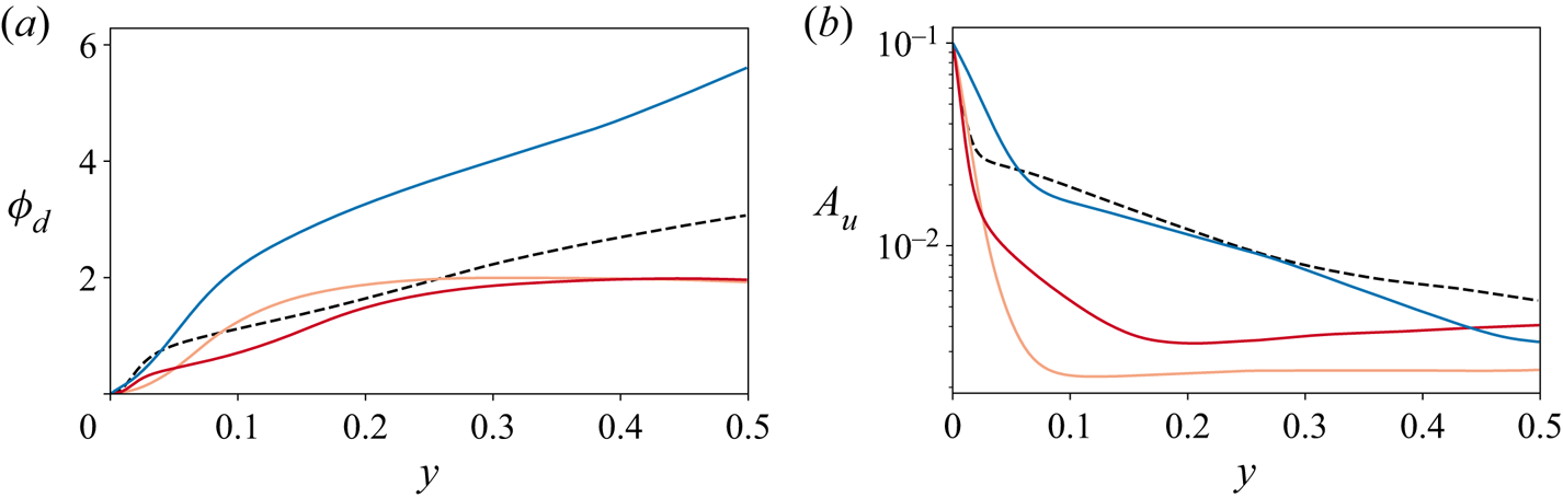
In contrast, the results for anti-cyclonic rotation ( $R_\varOmega >0$) do present more differences when compared to the non-rotating case. For
 $R_\varOmega =0.1$, the amplitude response drops very rapidly as we move away from the wall, and then remains constant from
 $y\ge 0.08$, while the phase delay also increases at first, and then remains constant from
 $y \ge 0.15$. The transition from one type of behaviour to the other happens at very different values of
 $y$, and the behaviour is very different from the constant velocity or constant exponential decay seen for
 $R_\varOmega \leq 0$, and also deviates strongly from the behaviour of the Stokes solution, namely linear phase increases and exponential amplitude decay. As we will justify further below, we can attribute this strange behaviour to the spanwise inhomogeneities introduced by the Taylor rolls, which introduce numerical artefacts and affect the calculation of
 $f$.
Turning to  $R_\varOmega =0.3$, we can observe the two near-wall and bulk regions, which have a linear behaviour for the phase delay and an exponential decaying behaviour for the amplitude response, as well as a third region for
 $y\ge 0.2$ that was unobserved previously and where both the phase delay and the amplitude response are constant. This indicates that rotation induces a region that is affected simultaneously and homogeneously by the flow modulations. Unlike for
 $R_\varOmega =0.1$, we believe that these results are not due to averaging artefacts, as they were also observed in the experiments by Verschoof et al. (Reference Verschoof, te Nijenhuis, Huisman, Sun and Lohse2018), who observed no significant dependence of
 $A_u$ and
 $\phi _d$ on
 $y$. As mentioned earlier, the set-up in Verschoof et al. (Reference Verschoof, te Nijenhuis, Huisman, Sun and Lohse2018) corresponds to an effective
 $R_\varOmega =0.286$, very close to our simulated value, and furthermore, the experiment measured
 $A_u$ and
 $\phi _d$ only at distances from the wall in the range
 $0.2< y<0.8$. According to our simulations, these distances would all correspond to the region where
 $A_u$ and
 $\phi _d$ are constant. This explains the discrepancy between our earlier results and the experiment: anti-cyclonic rotation adds a new physical phenomenon where the perturbation coming from the wall modulation appears to be constant throughout the bulk.
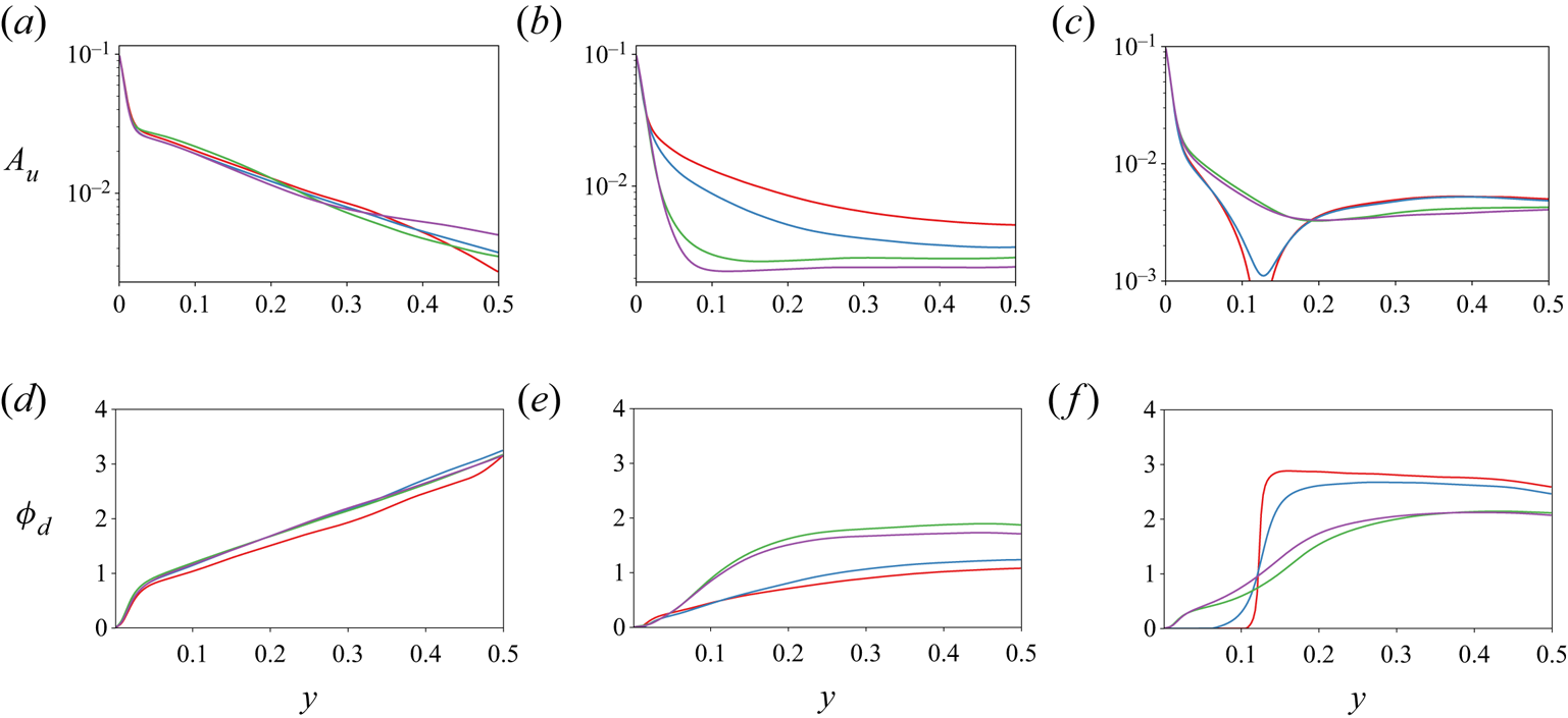
To justify further that the presence of large-scale structures interferes with the measurement of the perturbation amplitude and phase delay for  $R_\varOmega =0.1$, in figure 15 we show the effects of calculating
 $A_u$ and
 $\phi _d$ by averaging over only a fraction of the spanwise length. The non-rotating case is used as a baseline, which shows that even taking an eighth of the spanwise domain length as an averaging window leads to reasonable results if large-scale structures are not present. Once the rotation is increased to
 $R_\varOmega =0.1$, it is impossible to obtain results that do not depend on the extent of the spanwise averaging window. Increasing the domain size leads the amplitude response to drop rapidly for the same
 $y$-coordinate, as the effect of spanwise inhomogeneity contaminates the measurement of
 $f$. Finally, when
 $R_\varOmega$ is further increased to
 $0.3$, the Taylor rolls disappear, and while neither an eighth of the domain nor a quarter is enough to produce accurate results, the results from half and the full domain show very similar behaviour. We can thus use our results for
 $R_\varOmega =0.3$ with confidence.
(a–c) Amplitude response  $A_{u}$, and d–f) phase delay
 $\phi _d$, against wall distance for
 $Wo=44$ and (a,d)
 $R_\varOmega =0$, (b,e)
 $R_\varOmega =0.1$, and (c,f)
 $R_\varOmega =0.3$. The different lines denote different averaging windows for azimuthal velocity:
 $L_z/8$, red;
 $L_z/4$, dark blue;
 $L_z/2$, green; and full
 $L_z$ extent, purple.
We finish this section by showing in figure 16 the amplitude response as a function of  $Wo$ for several wall distances at
 $R_\varOmega =-0.1$ and
 $0.3$. For
 $R_\varOmega =-0.1$, we can observe results very similar to those seen for the non-rotating case, with a small region consistent with
 $A_u\sim Wo^{-2}$ behaviour. This shows that for cyclonic rotation, the physics of the flow's response to modulation remains largely unchanged.
Amplitude response ( $A_{u}$) against
 $Wo$ for
 $\alpha =0.1$ and (a)
 $R_\varOmega =-0.1$, and (b)
 $R_\varOmega =0.3$. For each plot, the black dashed line shows the scaling
 $A_u \sim Wo^{-2}$, and the inset shows a plot of the compensated amplitude
 $A_uWo^2$ against
 $Wo$ to emphasize the scaling. The grey vertical dashed lines mark
 $T_\tau=1$.
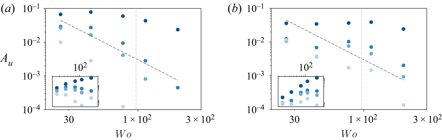
For  $R_\varOmega =0.3$, we cannot observe any behaviour consistent with power laws. We can compare this case to the experiments of Verschoof et al. (Reference Verschoof, te Nijenhuis, Huisman, Sun and Lohse2018), as there are some similarities. First, we can observe a similar collapse of
 $A_u$ for low
 $Wo$ at
 $0.05< y<0.5$, as well as a slow divergence of the curves as
 $Wo$ becomes larger. While in Verschoof et al. (Reference Verschoof, te Nijenhuis, Huisman, Sun and Lohse2018) this collapse held until
 $Wo>100$, in our case, the data can only really be seen to collapse for
 $Wo=26$. Furthermore, the experiments reported an exponential-like decay for
 $A_u$ as a function of
 $Wo$, but we do not observe behaviour consistent with exponential decay. The differences between the experiment and the simulations can probably be attributed to two sources. First, the experiments do not report data very close to the wall, so a fair comparison would not include the data points in the darkest blue. Second, the correct way to express the dimensionless period is not the viscosity-based
 $Wo$ but
 $T_\tau$, as the flow is fully turbulent. Therefore, it does not make sense to compare cases at the same
 $Wo$, but instead we should compare cases and flow behaviour transitions for the same values of
 $T_\tau$. In our simulations,
 $Wo\approx 80$ corresponds to
 $T_\tau =1$, while in the Verschoof et al. (Reference Verschoof, te Nijenhuis, Huisman, Sun and Lohse2018) experiments, we can expect this number to be closer to
 $Wo\approx 220$. Therefore, the separation of data that we see at
 $Wo\approx 40$ corresponds approximately to the separation of curves observed at
 $Wo\approx 110$ in the experiments, making the observation of
 $y$-independence for the amplitude response at large forcing periods consistent across simulations and experiments.
5. Summary and outlook
We performed direct numerical simulations (DNS) of non-rotating and rotating plane Couette flow with a modulated plate at a fixed shear Reynolds number  $Re_s= 3 \times 10^4$ for Womersley numbers in the range
 $Wo \in [26,200]$ while keeping the amplitude of the modulation constant at
 $\alpha =0.1$. We also studied the effect of cyclonic and anti-cyclonic Coriolis forces in the system by varying the rotation parameter
 $R_\varOmega$ in the range
 $[-0.1, 0.3]$.
The average shear at the walls and the instantaneous dissipation was found to be independent of the modulation frequency regardless of the Coriolis force added, and no evidence of resonance between flow structures and modulation was found, consistent with the RBC results of Jin & Xia (Reference Jin and Xia2008).
The propagation of the modulation was measured using Fourier transforms of phase-averaged velocities to obtain the phase delay and amplitude response. For the non-rotating case ( $R_\varOmega = 0$), both the modulation response amplitude and the phase delay show behaviour similar to the theoretical solution of Stokes’ boundary problem, i.e. a linear behaviour for the phase delay, and an exponential decay for the amplitude response. There are two main regimes, a near-wall regime where the effective viscosity is close to the fluid viscosity, and a bulk regime where the effective viscosity appears to be much higher. The transition between slopes is observed at
 $y\approx 0.05$, which corresponds to
 $y^+ = 40$ in viscous units, i.e. the transition between the viscid- and log-law regions of the turbulent boundary layer. When plotting the amplitude response as a function of
 $Wo$, we found a high-
 $Wo$ regime with behaviour consistent with the
 $A_u\sim Wo^{-2}$ behaviour, as is expected of modulated turbulence at high frequencies (von der Heydt et al. Reference von der Heydt, Grossmann and Lohse2003a). We also confirmed that the amplitude of the modulation is an unimportant parameter in determining the physics of the system for
 $\alpha <0.2$.
The simulations with cyclonic rotation result in behaviour similar to that of the non-rotating case: the modulation amplitude falls off exponentially at two different slopes, with the change of slope now occurring at  $y\approx 0.08$, which again happens to be at
 $y^+ = 40$ – the transition between the viscous sublayer and the buffer layer. Results for anti-cyclonic conditions were presented for
 $R_\varOmega = 0.1$ and
 $0.3$. For both anti-cyclonic conditions, the amplitude decay as a function of distance from the wall exhibits behaviour very different to the non-rotating case or cyclonic conditions, and deviates from Stokes’ solution. We attributed this marked difference at
 $R_\varOmega =0.1$ to the presence of Taylor rolls, which introduce spanwise inhomogeneities and prevent the adequate calculation of the amplitude response. Furthermore, for
 $R_\varOmega =0.3$, the amplitude decay and phase delay at
 $y\geq 0.2$ remain fairly constant and are consistent with the observations in Verschoof et al. (Reference Verschoof, te Nijenhuis, Huisman, Sun and Lohse2018). We conclude by noting that the correct non-dimensional time scale of modulated and rotating turbulent Couette flow is the frictional time scale
 $t_\tau$, and expressing the period as
 $T_\tau$ leads to good correspondence of the amplitude response behaviour between these current simulations and the experimental observations of Verschoof et al. (Reference Verschoof, te Nijenhuis, Huisman, Sun and Lohse2018).
The behaviour of the anti-cyclonic cases warrants further investigation, especially that seen at  $R_\varOmega =0.3$, which corresponds physically to a bulk region that feels the modulation all at once. Other types of modulation, such as periodic pulses, should also be analysed to find whether the average shear at the plates can be modified. To investigate these cases, more advanced ways of studying how the modulation propagates into the fluid must be developed, as the simple phase-averaged Fourier transform will not be able to produce adequate results.
Acknowledgements
We acknowledge the Research Computing Data Core (RCDC) at the University of Houston for providing us with computational resources and technical support.
Declaration of interests
The authors report no conflict of interest.


 Open access

