2.1 Relevant dimensionless parameters

A thin viscous film of initial average thickness $H_{i}^{\ast }$ coats the inside of a cylinder of inner radius $R$ whose axis is orthogonal to gravity (figure 1). The film aspect ratio $\unicode[STIX]{x1D6FF}=H_{i}^{\ast }/R$ is small, $\unicode[STIX]{x1D6FF}\ll 1$ . Defining $\unicode[STIX]{x1D707}$ as the dynamic viscosity, $\unicode[STIX]{x1D70C}$ the density and $g$ the gravitational field, the drainage time is given by the gravitational relaxation scale $\unicode[STIX]{x1D70F}_{d}=\unicode[STIX]{x1D707}R/(\unicode[STIX]{x1D70C}gH_{i}^{\ast 2})$ (Trinh et al. Reference Trinh, Kim, Hammoud, Howell, Chapman and Stone2014). The other relevant time scale of the problem is that of the classic RTI, $\unicode[STIX]{x1D70F}_{RT}$ , which is proportional to $\unicode[STIX]{x1D707}\unicode[STIX]{x1D6FE}/(\unicode[STIX]{x1D70C}^{2}g^{2}H_{i}^{\ast 3})$ (Fermigier et al. Reference Fermigier, Limat, Wesfreid, Boudinet and Quilliet1992), where $\unicode[STIX]{x1D6FE}$ is the fluid’s surface tension. Taking the ratio between these two times, we define the Bond number as $Bo=\unicode[STIX]{x1D70C}gH_{i}^{\ast }R/\unicode[STIX]{x1D6FE}$ , therefore accounting for the relative magnitude of gravitational and surface tension forces.

Figure 1.

Sketch of the three-dimensional problem geometry.

2.2 Experimental set-up

Experiments are performed with two types of silicone oil (Carl Roth GmbH) with kinematic viscosity $\unicode[STIX]{x1D708}=1000$  cSt, density $\unicode[STIX]{x1D70C}=970~\text{kg}~\text{m}^{-3}$ , surface tension $\unicode[STIX]{x1D6FE}=21.2~\text{mN}~\text{m}^{-1}$ and $\unicode[STIX]{x1D708}=5000$  cSt, $\unicode[STIX]{x1D70C}=973~\text{kg}~\text{m}^{-3}$ , $\unicode[STIX]{x1D6FE}=21.4~\text{mN}~\text{m}^{-1}$ , respectively. Two different techniques are adopted to obtain the initial uniform coating (see figure 2). The first one consists in using a poly(methyl methacrylate) (PMMA) cylinder partially filled with silicone oil and spinning it around its axis (see figure 2 a). Following Melo (Reference Melo1993), the critical rotation velocity $\unicode[STIX]{x1D6FA}_{c}$ above which a homogeneous film can be obtained is $\unicode[STIX]{x1D6FA}_{c}=(A/4.428R)^{2}g/\unicode[STIX]{x1D708}R$ , where $A$ is the cross-section of the cylinder occupied by the fluid. For $\unicode[STIX]{x1D6FA}\gg \unicode[STIX]{x1D6FA}_{c}$ , the film thickness is expected to be uniform, so that the liquid is in solid-body rotation with the cylinder; whereas for $\unicode[STIX]{x1D6FA}<\unicode[STIX]{x1D6FA}_{c}$ , different kinds of undesired instabilities can be observed (Thoroddsen & Mahadevan Reference Thoroddsen and Mahadevan1997; Hosoi & Mahadevan Reference Hosoi and Mahadevan1999; Pougatch & Frigaard Reference Pougatch and Frigaard2011; Seiden & Thomas Reference Seiden and Thomas2011). For the range of parameters under study, the threshold $\unicode[STIX]{x1D6FA}_{c}$ is always less than $100~\text{rpm}$ , the speed at which we operate. Furthermore, for this speed, inertial instabilities such as the ones studied by Benilov & Lapin (Reference Benilov and Lapin2013) do not form in our experiments. The relative non-uniformity of the film thickness is within $2\,\%$ . After the uniform film is obtained, the rotation is suddenly stopped so that the coating stops too with time scale $\unicode[STIX]{x1D70F}=H_{i}^{\ast 2}/\unicode[STIX]{x1D708}$ . Owing to the small film thickness and large viscosity, the time $\unicode[STIX]{x1D70F}$ is small compared to the gravitational drainage time $\unicode[STIX]{x1D70F}_{d}$ . More precisely, we get $0.4~\text{ms}<\unicode[STIX]{x1D70F}<16~\text{ms}$ and $0.55~\text{s}<\unicode[STIX]{x1D70F}_{d}<20.1~\text{s}$ , confirming $\unicode[STIX]{x1D70F}\ll \unicode[STIX]{x1D70F}_{d}$ . We can therefore assume that the gravity-induced drainage starts from a uniform stationary condition.

For the second technique (see figure 2 b), a uniform film of silicone oil is coated onto a planar PMMA plate with dimensions $500~\text{mm}\times 200~\text{mm}\times 4~\text{mm}$ using a film applicator (Film Casting Knife 15 cm, BYK GmbH), whose gap clearance can be tuned. The actual film thickness as well as its uniformity, which is within $4\,\%$ , are verified before proceeding. The film thickness is measured with a Confocal Chromatic Sensing technique (STIL CL2-MG140 and CL4-MG20 with CCS PRIMA), which allows measurements between $20$ and $4000~\unicode[STIX]{x03BC}\text{m}$ , with an accuracy of $250~\text{nm}$ (see appendix E for further details on the measurement technique). After coating, the plate is then turned upside down and bent by clamping its extremities. As a result, the upper part of the substrate – expected to be the key region – has a circular cross-section.

Figure 2.

(a) Cylindrical substrate formed by a PMMA cylinder of radius $R=8.6~\text{cm}$ and length $L_{z}=15~\text{cm}$ partially filled with silicone oil. The axis of the cylinder is mounted on a motor which can reach $100~\text{rpm}$ for coating purposes. (b) Curved PMMA plate of $500~\text{mm}\times 200~\text{mm}\times 4~\text{mm}$ clamped at its extremities to prescribe the desired substrate curvature. The thin film of silicone oil is applied with a film applicator prior to deforming the plate. Scale bars correspond to $10~\text{cm}$ . Rivulets are visible in both photographs.

The achievable parameter range for each method is reported in table 1. As evident from the table, the rotating cylinder is suitable for intermediate Bond numbers and relatively large film aspect ratios, whereas the curved plate allows for a slightly wider range of Bond numbers and smaller aspect ratios owing to its flexibility in tuning the plate curvature.

Table 1.

Values of relevant quantities for the experimentally explored parameter range.

A Basler camera (acA1300-60gm) with a long-focus zoom lens 18–108 mm $f/2.5$ (LMZ 45C5, Japan Lens Inc.) is employed to record the experiment. For the cylindrical set-up, we measured the temporal evolution of the film thickness at $\unicode[STIX]{x1D703}=0$ along the cylinder length of $L_{z}=15~\text{cm}$ (see figure 1). The optical pen, measuring the film thickness at $200~\text{Hz}$ , is mounted on a linear motor stage (Aerotech PRO165LM), which performs oscillatory motions at $0.4~\text{Hz}$ . Given the slow dynamics induced by the high viscosity of the fluid, a sufficient temporal and spatial resolution (0.6 mm) is thus achieved.

2.3 Phase diagram: rivulets or dripping droplets?

In the classical RTI for horizontal substrates, thin films eventually destabilize into droplets, either directly or following the formation of rolls and axisymmetric structures caused by the presence of the contact line at the boundaries or local perturbations (Fermigier et al. Reference Fermigier, Limat, Wesfreid, Boudinet and Quilliet1992). The orientation of these structures is dictated only by the boundaries of the geometry or initial conditions. The fate of thin films coating the concave side of a cylindrical substrate is qualitatively different, as patterns such as rivulets may persist over time, i.e. drops do not necessarily form. Aiming to classify the patterns observed in our experiments, we have built a phase diagram that we report in figure 3. As evident from the figure, the diagram divides into three main regions, which we now describe.

Dripping droplets arise in the limit of very large Bond numbers ( $Bo\gtrsim 200$ ) and vanishing film aspect ratios ( $\unicode[STIX]{x1D6FF}<10^{-2}$ ), that is, when the substrate may be seen as nearly horizontal on the scale of the film (see supplementary movie 1 available online at https://doi.org/10.1017/jfm.2017.817). Often, droplets arrange themselves on a hexagonal structure, as shown in the inset of figure 3. However, the initially formed two-dimensional array of droplets deforms over time following the drainage flow. Droplets were found to pinch off or slide along the substrate.

Rivulets are found for smaller Bond numbers, $Bo\lesssim 100$ (see figure 2 and supplementary movie 2), yet larger than the critical value, $Bo>12$ (Trinh et al. Reference Trinh, Kim, Hammoud, Howell, Chapman and Stone2014; Balestra et al. Reference Balestra, Brun and Gallaire2016). Unlike the rolls forming under a horizontal substrate, rivulets persist over time and do not further destabilize into droplets. These rivulets have a clear orientation dictated by the geometric anisotropy of the substrate curvature and are always orthogonal to the axis of the cylinder.

Dripping droplets and rivulets are separated by a mixed regime for Bond numbers of the order of $100$ , where both patterns coexist on the substrate: rivulets are typically found at the boundaries and droplets in the centre (see supplementary movie 3). For film aspect ratios $\unicode[STIX]{x1D6FF}>7\times 10^{-3}$ , rivulets are found to experience a secondary instability at later times and destabilize into several aligned droplets which pinch off, similar to the pinch-off studied by Indeikina, Veretennikov & Chang (Reference Indeikina, Veretennikov and Chang1997) and Alekseenko et al. (Reference Alekseenko, Aktershev, Bobylev, Kharlamov and Markovich2015) (see supplementary movie 4).

Figure 3.

Phase diagram as a function of the film aspect ratio $\unicode[STIX]{x1D6FF}$ and Bond number $Bo$ . Full symbols correspond to $\unicode[STIX]{x1D708}=1000~\text{cSt}$ and empty symbols to $\unicode[STIX]{x1D708}=5000~\text{cSt}$ . Numbers correspond to supplementary movies. The uncertainty on the film aspect ratio is of the order of $4\,\%$ (respectively $2\,\%$ ) for the curved plate (respectively cylinder) set-up and the uncertainty on the Bond number is of the order of $5\,\%$ . Insets: top view of the two-dimensional hexagonal pattern of droplets (left) and side view of rivulets (right). Scale bars correspond to 10 mm.

Experiments performed with the cylinder display a larger critical Bond number for the transition from rivulets to the mixed regime. The main reason is the smoother initial film thickness in this configuration compared to the curved plate set-up. As will become clear in § 4, the system is very sensitive to ambient noise and particular care has to be taken when performing the experiments. The thin-film evolutions in a cylinder for two different experiments with the same parameters are shown in supplementary movies 5 and 6, illustrating the reproducibility of the results.

In the phase diagram of figure 3, experiments with similar values of $(Bo,\unicode[STIX]{x1D6FF})$ and different viscosities collapse to the same region. This is an indication that viscosity does not seem to play a major role in pattern selection, while it modifies the time scale for the appearance of such a pattern. Note that in our problem the typical time scale of the Rayleigh–Plateau instability (Hammond Reference Hammond1983; Duclaux, Clanet & Quéré Reference Duclaux, Clanet and Quéré2006; Lister et al. Reference Lister, Rallison, King, Cummings and Jensen2006) is several orders of magnitude larger than the characteristic time of the classical RTI. In fact we have $\unicode[STIX]{x1D70F}_{RP}\sim \unicode[STIX]{x1D707}(R-H_{i}^{\ast })^{4}/(\unicode[STIX]{x1D6FE}H_{i}^{\ast 3})\sim \unicode[STIX]{x1D707}R/(\unicode[STIX]{x1D6FE}\unicode[STIX]{x1D6FF}^{3})$ for the Rayleigh–Plateau instability and $\unicode[STIX]{x1D70F}_{RT}\sim \unicode[STIX]{x1D707}\ell _{c}^{4}/(\unicode[STIX]{x1D6FE}H_{i}^{\ast 3})$ for the RTI, so that $\unicode[STIX]{x1D70F}_{RP}/\unicode[STIX]{x1D70F}_{RT}=(R/\ell _{c})^{4}\gg 1$ . Furthermore, the dominant wavelength (see figure 2 or the inset of figure 3) is found to be proportional to the capillary length in our experiments as another indication of the relevance of the RTI. Recall that for the Rayleigh–Plateau instability the wavelength is proportional to the cylinder radius. We thus argue that rivulets form following the gravitational RTI.

Note finally that perturbations invariant in the axial direction, or waves, as studied in Trinh et al. (Reference Trinh, Kim, Hammoud, Howell, Chapman and Stone2014) and Balestra et al. (Reference Balestra, Brun and Gallaire2016), are not observed in our experiments. In § 3 we propose a two-dimensional linear optimal transient growth analysis, for small aspect ratios, where we expect to identify the transition between rivulets and dripping droplets. Given the phase diagram in figure 3, we expect the value of the critical $Bo$ to be independent of $\unicode[STIX]{x1D6FF}$ for $\unicode[STIX]{x1D6FF}\lesssim 10^{-2}$ .

3.1 Governing equation

Owing to the small aspect ratio of the problem, $\unicode[STIX]{x1D6FF}\ll 1$ , we use a lubrication approach to model the evolution of the film thickness (Oron, Davis & Bankoff Reference Oron, Davis and Bankoff1997). Inertial effects are neglected due to the large viscosity of the fluid (the Reynolds number is of the order of $10^{-3}$ ). The flow is driven by the gravitational field and by the capillary pressure gradient. By using the local mass conservation in cylindrical coordinates as well as $H_{i}^{\ast }$ and $\unicode[STIX]{x1D70F}_{d}$ as length and time gauges of the problem, the governing equation for the dimensionless film thickness $\bar{H}$ for small aspect ratios reduces to (see appendix A for more details on the derivation)

(3.1) $$\begin{eqnarray}\bar{H}_{t}+{\displaystyle \frac{1}{3}}\!\left[\underbrace{\bar{H}^{3}}_{\text{IV}}\!\left(\underbrace{{\displaystyle \frac{1}{Bo}}\bar{\unicode[STIX]{x1D705}}_{\unicode[STIX]{x1D703}}}_{\text{I}}+\underbrace{\unicode[STIX]{x1D6FF}\bar{H}_{\unicode[STIX]{x1D703}}\cos \unicode[STIX]{x1D703}}_{\text{II}}+\underbrace{\sin \unicode[STIX]{x1D703}}_{\text{III}}\right)\right]_{\unicode[STIX]{x1D703}}\!+{\displaystyle \frac{1}{3\unicode[STIX]{x1D6FF}^{2}}}\!\left[\underbrace{\bar{H}^{3}}_{\text{IV}}\!\left(\underbrace{{\displaystyle \frac{1}{Bo}}\bar{\unicode[STIX]{x1D705}}_{z}}_{\text{I}}+\underbrace{\unicode[STIX]{x1D6FF}\bar{H}_{z}\cos \unicode[STIX]{x1D703}}_{\text{II}}\right)\right]_{z}\!=0,\end{eqnarray}$$

where indices represent partial derivatives and $\bar{\unicode[STIX]{x1D705}}$ is the curvature of the film interface. Terms $\text{I}$ represent surface tension effects, terms $\text{II}$ the variation of the hydrostatic pressure distribution, term $\text{III}$ accounts for the gravity-induced drainage and term $\text{IV}$ is the mobility of the liquid. The curvature up to the second order in $\unicode[STIX]{x1D6FF}$ is

(3.2) $$\begin{eqnarray}\displaystyle \bar{\unicode[STIX]{x1D705}} & = & \displaystyle {\displaystyle \frac{\bar{H}_{zz}}{(\bar{H}_{z}^{2}+1)^{3/2}}}+{\displaystyle \frac{\unicode[STIX]{x1D6FF}}{(\bar{H}_{z}^{2}+1)^{1/2}}}\nonumber\\ \displaystyle & & \displaystyle -\,\unicode[STIX]{x1D6FF}^{2}\left[{\displaystyle \frac{\bar{H}_{zz}\bar{H}_{\unicode[STIX]{x1D703}}^{2}}{2(\bar{H}_{z}^{2}+1)^{3/2}}}-{\displaystyle \frac{3\bar{H}_{z}^{2}\bar{H}_{zz}\bar{H}_{\unicode[STIX]{x1D703}}^{2}}{2(\bar{H}_{z}^{2}+1)^{5/2}}}+{\displaystyle \frac{2\bar{H}_{z}\bar{H}_{\unicode[STIX]{x1D703}z}\bar{H}_{\unicode[STIX]{x1D703}}}{(\bar{H}_{z}^{2}+1)^{3/2}}}-{\displaystyle \frac{\bar{H}_{\unicode[STIX]{x1D703}\unicode[STIX]{x1D703}}}{(\bar{H}_{z}^{2}+1)^{1/2}}}-{\displaystyle \frac{\bar{H}}{(\bar{H}_{z}^{2}+1)^{1/2}}}\right]\nonumber\\ \displaystyle & & \displaystyle +\,O(\unicode[STIX]{x1D6FF}^{3}).\end{eqnarray}$$

Inspired by the good agreement between the linear optimal transient growth analysis of the top region of the cylinder (Trinh et al. Reference Trinh, Kim, Hammoud, Howell, Chapman and Stone2014) with that of the entire circular geometry (Balestra et al. Reference Balestra, Brun and Gallaire2016), we concentrate on the cylinder’s most unstable region close to $\unicode[STIX]{x1D703}=0$ . For $\unicode[STIX]{x1D6FF}\ll 1$ , the change of variable $\unicode[STIX]{x1D703}=\unicode[STIX]{x1D6FF}^{1/2}x$ and $z=\unicode[STIX]{x1D6FF}^{-1/2}y$ is suitable. At leading order, the curvature reduces to $\bar{\unicode[STIX]{x1D705}}=\unicode[STIX]{x1D6FF}(1+\bar{H}_{xx}+\bar{H}_{yy})$ . In the limit $x\ll 1$ , the lubrication equation (3.1) becomes (see appendix B)

(3.3) $$\begin{eqnarray}\bar{H}_{t}+\unicode[STIX]{x1D735}\boldsymbol{\cdot }\left[{\displaystyle \frac{\bar{H}^{3}}{3}}\unicode[STIX]{x1D735}\left({\displaystyle \frac{1}{Bo}}\unicode[STIX]{x1D6FB}^{2}\bar{H}+\bar{H}+\underbrace{{\displaystyle \frac{x^{2}}{2}}}_{\text{III}}\right)\right]=0,\end{eqnarray}$$

where $\unicode[STIX]{x1D735}=[\unicode[STIX]{x2202}_{x},\unicode[STIX]{x2202}_{y}]^{\text{T}}$ is the gradient operator. Equation (3.3) differs from the classical lubrication equation employed for the horizontal substrate (Fermigier et al. Reference Fermigier, Limat, Wesfreid, Boudinet and Quilliet1992) only by the presence of the drainage term $\text{III}$ . This term breaks the symmetry of the problem and is the key to the following analysis.

3.2 Linear disturbance solution

For a uniform film thickness,  $\bar{H}(x,y,t)=H(t)$ , (3.3) has an analytical solution of the form (Takagi & Huppert Reference Takagi and Huppert2010; Trinh et al. Reference Trinh, Kim, Hammoud, Howell, Chapman and Stone2014; Lee et al. Reference Lee, Brun, Marthelot, Balestra, Gallaire and Reis2016)

(3.4) $$\begin{eqnarray}H(T)={\displaystyle \frac{1}{\sqrt{T}}},\end{eqnarray}$$

with $T=1+(2/3)t$ (see appendix C for the derivation). This solution will be shown to be asymptotically stable and we will refer to it as the drainage solution.

The film thickness is decomposed into this spatially uniform drainage solution $H(T)$ and small space-dependent disturbances $\unicode[STIX]{x1D700}h(x,y,T)$ :

(3.5) $$\begin{eqnarray}\bar{H}(x,y,T)=H(T)+\unicode[STIX]{x1D700}h(x,y,T),\quad \unicode[STIX]{x1D700}\ll 1.\end{eqnarray}$$

Entering the decomposition (3.5) into the lubrication equation (3.3) and considering first-order terms, we obtain the linear disturbance equation for the perturbations:

(3.6) $$\begin{eqnarray}h_{T}+{\displaystyle \frac{1}{2T^{3/2}}}\left({\displaystyle \frac{\unicode[STIX]{x1D6FB}^{4}h}{Bo}}+\unicode[STIX]{x1D6FB}^{2}h\right)+{\displaystyle \frac{3}{2T}}(xh_{x}+h)=0.\end{eqnarray}$$

In this expression, the base flow $H$ is explicitly accounted for by the powers of $T$ . For an initially harmonic disturbance $h(x,y,1)=h_{0}(x,y)=\exp [\text{i}(\unicode[STIX]{x1D6FC}x+\unicode[STIX]{x1D6FD}y)]+\text{c.c.}$ with wavenumber $\unicode[STIX]{x1D6FC}$ in the polar direction and $\unicode[STIX]{x1D6FD}$ in the axial direction, the solution is

(3.7) $$\begin{eqnarray}h(x,y,T)=A(\unicode[STIX]{x1D6FC},\unicode[STIX]{x1D6FD},T)\exp \left[\text{i}\left(\unicode[STIX]{x1D6FC}{\displaystyle \frac{x}{T^{3/2}}}+\unicode[STIX]{x1D6FD}y\right)\right]+\text{c.c.},\end{eqnarray}$$

where $A$ satisfies

(3.8) $$\begin{eqnarray}A_{T}+{\displaystyle \frac{1}{2}}\left[{\displaystyle \frac{1}{Bo}}\left({\displaystyle \frac{\unicode[STIX]{x1D6FC}^{4}}{T^{15/2}}}+{\displaystyle \frac{\unicode[STIX]{x1D6FD}^{4}}{T^{3/2}}}+2{\displaystyle \frac{\unicode[STIX]{x1D6FC}^{2}\unicode[STIX]{x1D6FD}^{2}}{T^{9/2}}}\right)-\left({\displaystyle \frac{\unicode[STIX]{x1D6FC}^{2}}{T^{9/2}}}+{\displaystyle \frac{\unicode[STIX]{x1D6FD}^{2}}{T^{3/2}}}\right)+{\displaystyle \frac{3}{T}}\right]A=0.\end{eqnarray}$$

The temporal dependence of the apparent wavenumber in the polar direction, $x/T^{3/2}$ , is chosen so as to annihilate the stretching term $xh_{x}$ in (3.6). The solution

(3.9) $$\begin{eqnarray}\displaystyle A(\unicode[STIX]{x1D6FC},\unicode[STIX]{x1D6FD},T) & = & \displaystyle {\displaystyle \frac{1}{T^{3/2}}}\exp \Bigg[\left(1-{\displaystyle \frac{1}{T^{7/2}}}\right){\displaystyle \frac{\unicode[STIX]{x1D6FC}^{2}}{7}}-{\displaystyle \frac{1}{Bo}}\left(1-{\displaystyle \frac{1}{T^{13/2}}}\right){\displaystyle \frac{\unicode[STIX]{x1D6FC}^{4}}{13}}\nonumber\\ \displaystyle & & \displaystyle +\,\left(1-{\displaystyle \frac{1}{T^{1/2}}}\right)\unicode[STIX]{x1D6FD}^{2}-{\displaystyle \frac{1}{Bo}}\left(1-{\displaystyle \frac{1}{T^{1/2}}}\right)\unicode[STIX]{x1D6FD}^{4}\nonumber\\ \displaystyle & & \displaystyle -\,{\displaystyle \frac{1}{Bo}}\left(1-{\displaystyle \frac{1}{T^{7/2}}}\right){\displaystyle \frac{2\unicode[STIX]{x1D6FC}^{2}\unicode[STIX]{x1D6FD}^{2}}{7}}\Bigg]\end{eqnarray}$$

is composed of two parts. On the one hand, the exponential term results from the RTI, with both destabilizing terms in $\unicode[STIX]{x1D6FC}^{2}$ or $\unicode[STIX]{x1D6FD}^{2}$ and stabilizing terms in $\unicode[STIX]{x1D6FC}^{4}$ , $\unicode[STIX]{x1D6FD}^{4}$ or $\unicode[STIX]{x1D6FC}^{2}\unicode[STIX]{x1D6FD}^{2}$ . This exponential term saturates to a maximal amplitude due to the thinning of the film, accounted for by the powers of $T$ . The largest amplitude depends only on the wavenumbers and on the Bond number. On the other hand, the gravity-induced drainage also enters through the algebraic term $1/T^{3/2}$ , which eventually makes the amplitude vanish for large times, $\lim _{T\rightarrow \infty }A(\unicode[STIX]{x1D6FC},\unicode[STIX]{x1D6FD},T)=0$ . In view of (3.9), it is therefore clear that the system is linearly asymptotically stable and only a transient growth can be achieved.

The initial amplitude evolution is given by

(3.10) $$\begin{eqnarray}A(\unicode[STIX]{x1D6FC},\unicode[STIX]{x1D6FD},T\rightarrow 1)\sim 1+{\displaystyle \frac{(\unicode[STIX]{x1D6FC}^{2}+\unicode[STIX]{x1D6FD}^{2}-3)Bo-(\unicode[STIX]{x1D6FC}^{2}+\unicode[STIX]{x1D6FD}^{2})^{2}}{2Bo}}(T-1)+O[T-1]^{2}.\end{eqnarray}$$

Introducing the oblique mode $\boldsymbol{k}=\unicode[STIX]{x1D6FC}\,\boldsymbol{e}_{x}+\unicode[STIX]{x1D6FD}\,\boldsymbol{e}_{y}$ , with norm $k=\sqrt{\unicode[STIX]{x1D6FC}^{2}+\unicode[STIX]{x1D6FD}^{2}}$ , initial growth occurs only if $k^{2}-3-k^{4}/Bo>0$ . This condition is best met for

(3.11) $$\begin{eqnarray}k_{0}=\sqrt{Bo/2},\end{eqnarray}$$

which is the initially most amplified wavenumber. In agreement with Trinh et al. (Reference Trinh, Kim, Hammoud, Howell, Chapman and Stone2014) and Balestra et al. (Reference Balestra, Brun and Gallaire2016), we thus recover the condition $Bo>12$ . We conclude that the threshold of the initial growth is not dependent on perturbation direction and the wavenumber $k_{0}$ corresponds to the wavenumber with the largest linear growth in the planar RTI (Fermigier et al. Reference Fermigier, Limat, Wesfreid, Boudinet and Quilliet1992).

In our formalism, waves and rivulets correspond to modes with $\boldsymbol{k}=\unicode[STIX]{x1D6FC}\,\boldsymbol{e}_{x}$ and $\boldsymbol{k}=\unicode[STIX]{x1D6FD}\,\boldsymbol{e}_{y}$ , respectively. The time evolution of the amplitude of waves and rivulets for the initial wavenumber of norm $k_{0}$ are shown in figure 4 for different Bond numbers. The growth of rivulets is much stronger than that of waves, and they persist longer, thereby rationalizing why waves are never seen in experiments. Note that waves and rivulets are the two limiting cases, as more generic perturbations can be expressed as a linear combination of $\unicode[STIX]{x1D6FC}$ and $\unicode[STIX]{x1D6FD}$ such that $\boldsymbol{k}=\unicode[STIX]{x1D6FC}\,\boldsymbol{e}_{x}+\unicode[STIX]{x1D6FD}\,\boldsymbol{e}_{y}$ .

Figure 4.

Linear perturbative results. The amplitude $A$ is shown for waves ( $\unicode[STIX]{x1D6FD}=0$ ) and rivulets ( $\unicode[STIX]{x1D6FC}=0$ ). They correspond to an initial perturbation with $k=k_{0}$ (see (3.11)) for Bond numbers $Bo=10$ , $30$ , $50$ , $70$ , $90$ and $110$ . Stars denote the largest amplitudes.

3.3 Optimal growth

The optimization of the perturbations modes is performed for pure $\unicode[STIX]{x1D6FC}$ and pure $\unicode[STIX]{x1D6FD}$ modes separately. The optimal wavenumbers and the optimal times correspond to the wavenumbers and times for which the amplitude is the largest.

Following (3.9) we find that the optimal wavenumber for the waves is

(3.12) $$\begin{eqnarray}\left.{\displaystyle \frac{\unicode[STIX]{x2202}A}{\unicode[STIX]{x2202}\unicode[STIX]{x1D6FC}}}\right|_{\unicode[STIX]{x1D6FD}=0}=0\quad \Longleftrightarrow \quad \unicode[STIX]{x1D6FC}_{max}(T)=\sqrt{{\displaystyle \frac{13}{14}}{\displaystyle \frac{(1-T^{-7/2})}{(1-T^{-13/2})}}Bo},\end{eqnarray}$$

whereas for the rivulets it is

(3.13) $$\begin{eqnarray}\left.{\displaystyle \frac{\unicode[STIX]{x2202}A}{\unicode[STIX]{x2202}\unicode[STIX]{x1D6FD}}}\right|_{\unicode[STIX]{x1D6FC}=0}=0\quad \Longleftrightarrow \quad \unicode[STIX]{x1D6FD}_{max}=\sqrt{{\displaystyle \frac{Bo}{2}}}.\end{eqnarray}$$

Hence, the wavenumber for the rivulets to reach the largest growth at any time always corresponds to the classical RTI most amplified wavenumber $k_{0}$ . The optimal wavenumber for waves has a weak dependence on the optimization time and tends to $k_{0}\sqrt{13/7}$ for large time horizons (see inset in figure 5 a). The largest growths reached by waves and rivulets as a function of time are therefore

(3.14) $$\begin{eqnarray}\displaystyle & \displaystyle A_{\unicode[STIX]{x1D6FC}_{max}}(T)=A(\unicode[STIX]{x1D6FC}_{max},0,T)={\displaystyle \frac{1}{T^{3/2}}}\exp \left[{\displaystyle \frac{13}{196}}{\displaystyle \frac{\left(1-T^{-7/2}\right)^{2}}{\left(1-T^{-13/2}\right)}}Bo\right], & \displaystyle\end{eqnarray}$$

(3.15) $$\begin{eqnarray}\displaystyle & \displaystyle A_{\unicode[STIX]{x1D6FD}_{max}}(T)=A(0,\unicode[STIX]{x1D6FD}_{max},T)={\displaystyle \frac{1}{T^{3/2}}}\exp \left[{\displaystyle \frac{1}{4}}(1-T^{-1/2})Bo\right]. & \displaystyle\end{eqnarray}$$

Solving $\unicode[STIX]{x2202}A_{\unicode[STIX]{x1D6FC}_{max}}/\unicode[STIX]{x2202}T=0$ and $\unicode[STIX]{x2202}A_{\unicode[STIX]{x1D6FD}_{max}}/\unicode[STIX]{x2202}T=0$ yields the times at which the amplitude is the largest. For rivulets, one finds $T_{A_{max}^{\unicode[STIX]{x1D6FD}}}=(Bo/12)^{2}$ and the largest linear transient growth of rivulets is thus

(3.16) $$\begin{eqnarray}A_{max}^{\unicode[STIX]{x1D6FD}}=\left({\displaystyle \frac{12}{Bo}}\right)^{3}\exp \left({\displaystyle \frac{1}{4}}Bo-3\right).\end{eqnarray}$$

The time optimization for waves yields an irreducible polynomial of degree $25$ that does not have an algebraic solution. The numerical solution shows that $T_{A_{max}^{\unicode[STIX]{x1D6FC}}}$ follows a power law with exponent close to $0.2$ for the considered Bond-number range. The largest linear transient growth that the waves can achieve for large Bond numbers scales as

(3.17) $$\begin{eqnarray}A_{max}^{\unicode[STIX]{x1D6FC}}\sim \exp \left({\displaystyle \frac{13}{196}}Bo\right)\quad \text{for }Bo\gg 12.\end{eqnarray}$$

The optimal times, as well as the corresponding largest amplitudes, are reported in figure 5. This optimization procedure confirms what has been observed in figure 4. The optimal times and amplitudes of the rivulets are much greater than those of the waves. Waves are stretched by the draining flow, see (3.7), reducing the time available for the instability to grow. The stretching effect is evidenced by the different temporal evolutions of the stabilizing and destabilizing RTI terms in (3.9). In contrast, rivulets only experience the thinning of the film, without being stretched along their characteristic direction. They grow for longer times and therefore reach larger amplitudes.

Figure 5.

(a) Times $T_{A_{max}}=\{T_{A_{max}^{\unicode[STIX]{x1D6FC}}},T_{A_{max}^{\unicode[STIX]{x1D6FD}}}\}$ corresponding to the largest amplitude $A_{max}=\{A_{max}^{\unicode[STIX]{x1D6FC}},A_{max}^{\unicode[STIX]{x1D6FD}}\}$ obtained by perturbing with the optimal wavenumbers $k_{max}=\{\unicode[STIX]{x1D6FC}_{max},\unicode[STIX]{x1D6FD}_{max}\}$ as a function of the Bond number. Inset: optimal wavenumbers rescaled by the horizontal RTI wavenumber $k_{0}$ as a function of time. (b) Largest achievable amplitudes $A_{max}$ as a function of the Bond number. Black dashed lines correspond to the high-Bond-number limit evolutions. Note that the disturbance amplitude $\unicode[STIX]{x1D700}A$ needs to be smaller than the base flow of order unity for the linear theory to hold.

3.4 Linear prediction

Equipped with the results of the linear optimal transient growth (summarized in table 2), we aim to better understand our experimental results. In particular, we consider the linear evolution of rivulets, $h_{0}(x,y)=\exp (\text{i}k_{0}y)+\text{c.c.}$ , waves, $h_{0}(x,y)=\exp (\text{i}k_{0}x)+\text{c.c.}$ , and hexagons having one vector aligned with the axis of the cylinder,

(3.18) $$\begin{eqnarray}h_{0}(x,y)={\textstyle \frac{1}{3}}\{\exp (\text{i}k_{0}y)+\exp [\text{i}({\textstyle \frac{1}{2}}\sqrt{3}k_{0}x-{\textstyle \frac{1}{2}}k_{0}y)]+\exp [\text{i}(-{\textstyle \frac{1}{2}}\sqrt{3}k_{0}x-{\textstyle \frac{1}{2}}k_{0}y)]\}+\text{c.c.},\end{eqnarray}$$

with $\unicode[STIX]{x1D6FC}=\unicode[STIX]{x1D6FD}=k_{0}$ the initially most amplified wavenumber, and we choose an initial perturbation with amplitude $\unicode[STIX]{x1D700}=10^{-3}$ . The linear theory holds as long as the magnitude of the disturbances $\unicode[STIX]{x1D700}A$ is smaller than the base flow, which is of order unity; see (3.5).

Figure 6.

Amplitude evolution of rivulets, waves and hexagons for (a)  $Bo=60$ and (b) $Bo=160$ . Thin dashed lines indicate necessary amplification of disturbances to become of order one when $\unicode[STIX]{x1D700}=10^{-3}$ . Given the asymptotic stability of the system, the amplitude of all initial conditions saturates and tends to zero for large times, which is the reason why only the evolution for $T\leqslant 20$ is presented here.

Table 2.

Summary of main results of the linear optimal transient growth analysis.

We find that, for low Bond numbers, $Bo\simeq 60$ , rivulets experience a linear growth strong enough for the perturbation to become of the order of the base flow (see figure 6 a), while the waves remain much smaller. The hexagons experience a large linear growth since they contain a rivulet mode. However, their amplitude remains smaller than one-third of that of the rivulets. For larger Bond numbers, e.g. $Bo=160$ in figure 6(b), rivulets, hexagons as well as waves experience a similar linear growth up to the amplitude where nonlinear effects become relevant. Thereby, for sufficiently large Bond numbers, the instability pattern is selected only by the nonlinear effects. Conversely, linear growth selects the pattern for low Bond numbers. Note that the critical Bond number at which nonlinear effects enter into play before the linear growth has promoted a specific pattern is dependent on perturbation amplitude. The experimental threshold of $Bo\sim 100$ , corresponding to the mixed regime of figure 3, is related to our experimental settings.

5.1 Nonlinear simulations at the top of the cylinder

In order to gain more insight into the dynamics of the rivulets, numerical simulations of the one-dimensional lubrication equation for the film thickness at the top of the cylinder are carried out ( $\unicode[STIX]{x1D703}=0$ ). The lubrication equation (3.1) at $\unicode[STIX]{x1D703}=0$ with vanishing polar derivatives reads

(5.1) $$\begin{eqnarray}\bar{H}_{t}+\underbrace{{\displaystyle \frac{1}{3}}\bar{H}^{3}}_{\text{I}}+\underbrace{{\displaystyle \frac{1}{3\unicode[STIX]{x1D6FF}^{2}}}\left[\bar{H}^{3}\left({\displaystyle \frac{1}{Bo}}\bar{\unicode[STIX]{x1D705}}_{z}+\unicode[STIX]{x1D6FF}\bar{H}_{z}\right)\right]_{z}}_{\text{II}}=0.\end{eqnarray}$$

The term labelled $\text{I}$ results from the drainage term in (3.1) and is responsible for the thinning of the film over time. The terms labelled $\text{II}$ match the classical terms of the equation describing the classical horizontal RTI (Fermigier et al. Reference Fermigier, Limat, Wesfreid, Boudinet and Quilliet1992). Equation (5.1) can be resolved numerically (see appendix D.2 for details) and its solution is validated by comparison with a two-dimensional nonlinear numerical simulation in figure 10(b). The domain size is $L_{z}=2\times 2\unicode[STIX]{x03C0}/b_{0}$ , with $b_{0}=k_{0}\unicode[STIX]{x1D6FF}^{1/2}=\sqrt{Bo\unicode[STIX]{x1D6FF}/2}$ the linear optimal wavenumber in the physical $z$ -space and the initial condition is $\bar{H}_{0}=1+\unicode[STIX]{x1D700}\cos (b_{0}z)$ . Periodic boundary conditions are used. An example of nonlinear evolution given by (5.1) is presented in figure 10. The narrow rivulets, whose peaks grow initially in time, are separated by a rather flat thin-film region (see figure 10 b).

Figure 10.

Nonlinear simulations at $\unicode[STIX]{x1D703}=0$ , i.e. using (5.1). Film thickness as a function of time for rivulets with optimal initial disturbance $\bar{H}_{0}=1+0.01\cos (b_{0}z)$ with $b_{0}=\sqrt{Bo\unicode[STIX]{x1D6FF}/2}$ . (a) Spatio-temporal map of the film thickness $\bar{H}$ . Dash-dotted and dashed lines correspond to the locations of the peaks and valleys, respectively, whose thickness evolution is shown in figure 12(a). (b) Profiles of $\bar{H}$ at successive times $t=0,2,\ldots ,20$ . The black dashed line corresponds to the nonlinear solution at $\unicode[STIX]{x1D703}=0$ and $t=20$ obtained when considering the entire circular geometry $-\unicode[STIX]{x03C0}<\unicode[STIX]{x1D703}<\unicode[STIX]{x03C0}$ , equation (3.1). Here $Bo=70$ and $\unicode[STIX]{x1D6FF}=0.02$ .

The nonlinear perturbation solution is given by $h(z,t)=[\bar{H}(z,t)-H(t)]/\unicode[STIX]{x1D700}$ , where $H(t)=(1+2t/3)^{-1/2}$ is the drainage solution at $\unicode[STIX]{x1D703}=0$ introduced in (3.4) and $\bar{H}(z,t)$ is obtained by the numerical resolution of (5.1). The amplitudes of the different harmonics can be found by the Fourier series decomposition of the perturbation $h$ :

(5.2) $$\begin{eqnarray}h(z,t)=\mathop{\sum }_{n\in \mathbb{N}}A_{n}(t)\exp (\text{i}nb_{0}z)+\text{c.c.}\end{eqnarray}$$

Results are presented in figure 11(a). The fundamental mode, $A_{1}$ , obtained via nonlinear simulations agrees well with our linear prediction for small values of $\unicode[STIX]{x1D700}$ . Nonetheless, for larger initial perturbations, $A_{1}$ is found to saturate and to subsequently decrease well before the linear prediction $A$ does. Albeit $\Vert A\Vert _{2}$ and $A_{1}$ mostly agree, that is, $A_{0}$ and higher harmonics do not contribute significantly to the energy, as evident from figure 11(b), we argue that their interaction with $A_{1}$ generates the observed saturation and therefore cannot be neglected. This type of stabilizing effect is in agreement with the aforementioned analysis of Fermigier et al. (Reference Fermigier, Limat, Wesfreid, Boudinet and Quilliet1992) for rolls. Note that, the larger the initial disturbance amplitude, the earlier the higher harmonics will influence the dynamics of the fundamental mode. Yet, if the amplitude is sufficiently small, the transient growth nature of the instability guarantees that the linear prediction holds for all times (not shown in figure 11(a), the linear evolution remains superimposed on the nonlinear evolution for $\unicode[STIX]{x1D700}=10^{-5}$ and $T>10$ ). The perturbation amplitude saturates and eventually vanishes due to the asymptotic stability of the system.

Figure 11.

(a) Linear (green solid line) and nonlinear (blue dashed lines) amplitudes of the fundamental, together with the total nonlinear amplitude (red solid lines) for the optimal initial disturbance $\bar{H}_{0}=1+\unicode[STIX]{x1D700}\cos (b_{0}z)$ with $b_{0}=\sqrt{Bo\unicode[STIX]{x1D6FF}/2}$ and different initial disturbance amplitudes $\unicode[STIX]{x1D700}=10^{-5}$ , $10^{-4}$ , $10^{-3}$ and $10^{-2}$ . Here $Bo=70$ and $\unicode[STIX]{x1D6FF}=0.02$ . (b) Evolution of the total nonlinear disturbance energy $\Vert A\Vert _{2}$ together with the relative amplitude of the different harmonics $A_{n}$ of (5.2). Here $\unicode[STIX]{x1D700}=10^{-3}$ , $Bo=70$ and $\unicode[STIX]{x1D6FF}=0.02$ .

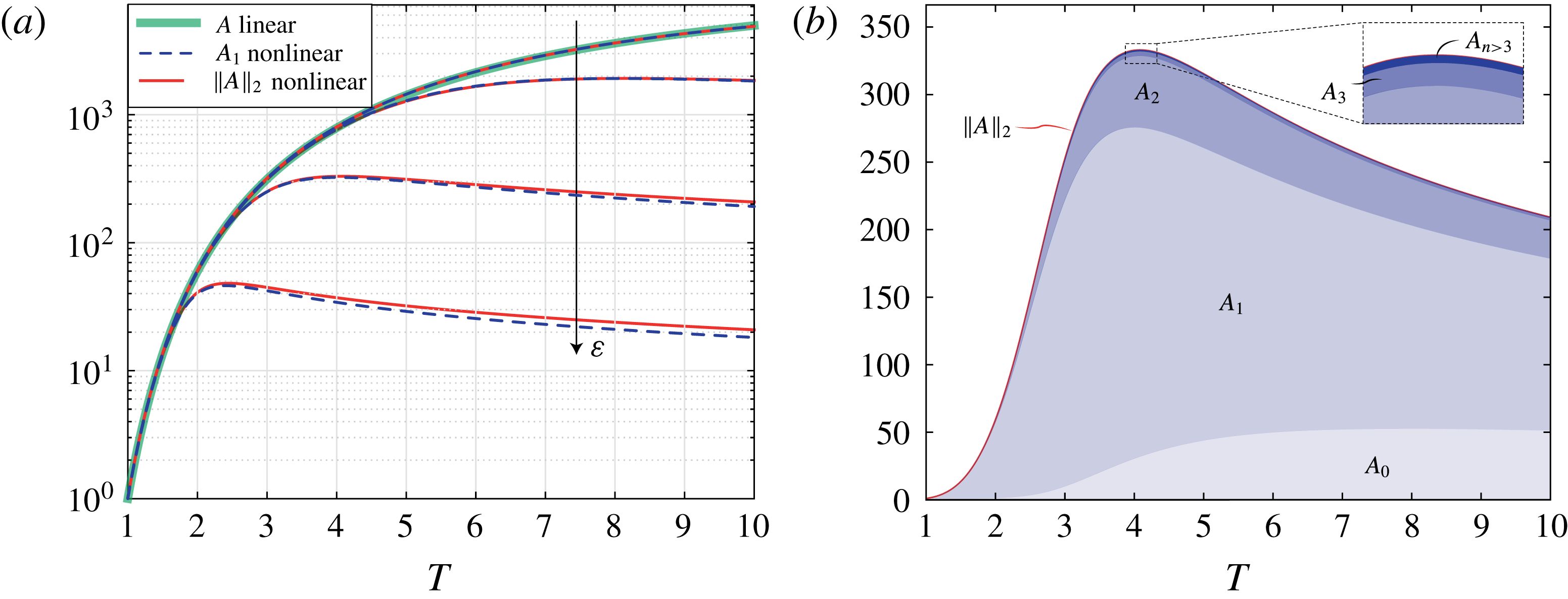
Despite their small contribution to $\Vert A\Vert _{2}$ , the higher-order harmonics are visible in our system. In figure 10(b), one can see that the flat regions between two fundamentals are subject to an instability too. This phenomenon is akin to the cascade of structures observed by Boos & Thess (Reference Boos and Thess1999) for the Marangoni instability in a thin film.

Our nonlinear analysis also indicates a modification in the base flow. We found that the mean film thickness of the perturbed film is smaller than the one of the draining solution $H(t)=1/\sqrt{1+2\,t/3}$ (Takagi & Huppert Reference Takagi and Huppert2010; Trinh et al. Reference Trinh, Kim, Hammoud, Howell, Chapman and Stone2014; Lee et al. Reference Lee, Brun, Marthelot, Balestra, Gallaire and Reis2016) (see figure 12 a). The development of rivulets hastens the drainage, which results from the coupling between the shape of the rivulets and the strong variation in the mobility of the liquid that scales as the cube of the local thickness, see (3.1). Initially, the different components of the thickness follow the linear evolution. There is no correction of the drainage solution due to the rivulets at early times. Nonetheless, when the higher harmonics come into play, $A_{0}$ is no longer vanishing (see figure 11 b). Building upon this observation, forcing the formation of rivulets is advantageous if one wishes to accelerate the drainage. Similar effects exist when waves run down at the surface of a liquid film flowing down an inclined plane (Kofman, Ruyer-Quil & Mergui Reference Kofman, Ruyer-Quil and Mergui2016). Such a modification of the mean flow is also a key to the saturation of hydrodynamic instabilities like vortex shedding in the wake flow behind a cylinder (Maurel, Pagneux & Wesfreid Reference Maurel, Pagneux and Wesfreid1995; Mantič-Lugo, Arratia & Gallaire Reference Mantič-Lugo, Arratia and Gallaire2014).

Figure 12.

(a) Film thickness evolutions at the peaks (red dash-dotted line) and valleys (green dashed line) of the rivulets shown in figure 10. The thick black solid line corresponds to the pure drainage solution $H$ and the blue dotted line to the mean film thickness $\langle \bar{H}\rangle$ . (b) Long-time evolutions for peaks, valleys and the pure drainage solution. Here $Bo=70$ , $\unicode[STIX]{x1D6FF}=0.02$ and $\unicode[STIX]{x1D700}=10^{-2}$ .

Moving away from the mean value of the film thickness, we now describe the evolution of the film thickness evolution in the peaks and valleys shown in figure 12. The growth of the peaks is fed by liquid extracted from the valleys. This mechanism is similar to the rolls in the planar RTI (Fermigier et al. Reference Fermigier, Limat, Wesfreid, Boudinet and Quilliet1992; Weidner, Schwartz & Eres Reference Weidner, Schwartz and Eres1997; Lister et al. Reference Lister, Rallison and Rees2010) or to the collars in the instability of a thin annular film coating the inside or outside of a cylinder in the absence of gravity (Hammond Reference Hammond1983; Lister et al. Reference Lister, Rallison, King, Cummings and Jensen2006). However, due to the thinning of the film in time, rivulets can only grow at short times. At later stages, the film thins and thus limits the liquid that a rivulet can pull from its vicinity. We find that, before the film becomes uniform again, the thickness in the valleys follow the scaling $t^{-1/4}$ (see figure 12 b). The same scaling was found by Lister et al. (Reference Lister, Rallison and Rees2010) for thin regions between pendent drops below planar substrates and for the lobes inside a cylinder studied by Hammond (Reference Hammond1983). At these intermediate times, the drainage of the rivulet valleys is driven by the classical RTI term $\text{II}$ in (5.1), yielding $\bar{H}\sim t^{-1/4}$ , as the effect of the term $\text{I}$ is negligible. For peaks, the term $\text{I}$ of (5.1) is not negligible, as the film thicknesses $\bar{H}$ is relatively larger. Eventually, the film thickness becomes uniform again due to the drainage in the rivulets and the drainage scales like the base flow, $\bar{H}\sim t^{-1/2}$ .

5.2 Experimental measurements

Rivulets are characterized experimentally by measuring the film thickness at the top of the cylinder. The spatio-temporal film thickness map is shown in figure 13(a). Rivulets first form at the boundaries of the cylinder where the film is perturbed by the existence of a meniscus. They then progressively invade the entire domain (see figure 13 b). As time evolves, the thickness of the rivulets eventually decreases, but their structure does not destabilize and we do not see any drops forming.

The rivulets were found to be almost equally spaced in experiments, with wavelength $\unicode[STIX]{x1D706}=14\pm 1~\text{mm}$ . The linearly most amplified wavelength is $\unicode[STIX]{x1D706}_{max}^{\unicode[STIX]{x1D6FD}}=2\unicode[STIX]{x03C0}/\sqrt{Bo\,\unicode[STIX]{x1D6FF}/2}H_{i}^{\ast }=13.5~\text{mm}$ (see § 3.3). Keeping in mind that the calculation leading to this value is idealized – infinite domain approximation – we find that the agreement is satisfactory. In reality, rivulets grow in a finite domain whose width is not an integer multiple of the most amplified wavelength, which they progressively invade starting from the boundaries. The profiles in figure 13(b) are qualitatively similar to their numerical counterpart. In particular the aforementioned higher harmonics are evident in the valleys between the rivulets. The detailed evolution of film thickness along the peaks and valleys is shown in figure 14(b). The trend of these curves is similar to that found numerically (see figure 12 a). Rivulets undergo a transient growth, whose magnitude decreases as we move towards the centre of the sample. The RTI propagates from the boundaries, where it is forced by a meniscus or a contact line. Limat et al. (Reference Limat, Jenffer, Dagens, Touron, Fermigier and Wesfreid1992) have shown that the front velocity of rolls predicted by the linear marginal stability criterion is given by $v_{f}=0.54\,(H^{\ast })^{3}(\unicode[STIX]{x1D70C}g)^{3/2}/\unicode[STIX]{x1D707}\unicode[STIX]{x1D6FE}^{1/2}$ , corresponding to the pulled fronts of Van Saarloos (Reference Van Saarloos2003). Such a front velocity model would predict a linear propagation of the front position in time. In experiments the front velocity reduces with time – the white lines from linear theory as reported in figure 13(a) are concave up. We hypothesize that this effect is caused by drainage, which effectively lowers $H^{\ast }$ as time goes by: $H^{\ast }(t^{\ast })=H_{i}^{\ast }/\sqrt{1+2\,t^{\ast }/3}$ . We have successfully reproduced the effect of the lateral boundaries on the inward propagation of rivulets using a periodic but inhomogeneous initial condition, as described in § 5.3.

Figure 13.

(a) Spatio-temporal diagram of the film thickness $\bar{H}^{\ast }$ measured experimentally along the cylinder generatrix at $\unicode[STIX]{x1D703}=0$ . Solid and dashed lines correspond to the locations of the peaks and valleys, respectively, whose thickness evolutions are shown in figure 14(b). The white line corresponds to the invading front location $z_{f}^{\ast }$ predicted by the linear theory. The film thickness close to the extremities of the cylinder is not shown in the spatio-temporal diagram due to measurement uncertainties induced by the large thickness gradients. (b) Profiles of $\bar{H}$ at successive times $t=30,60,\ldots ,270~\text{s}$ for a range of dimensional axial locations $z^{\ast }\in [-61,0]~\text{mm}$ . The Bond number is approximatively $67$ and the film aspect ratio $0.02$ .

Figure 14.

(a) Evolution of the mean film thickness $\langle \bar{H}^{\ast }\rangle$ obtained experimentally (blue dashed line) and numerically (orange thin line) compared to the uniform pure draining solution $H^{\ast }(t^{\ast })=H_{i}^{\ast }/\sqrt{1+2\,t^{\ast }/3}$ (thick black solid line). (b) Film thickness evolutions at the peaks (solid lines) and valleys (dashed lines) of the rivulets shown in figure 13(a). The location in mm is shown in the legend. The thick black solid line corresponds to the pure drainage solution $H^{\ast }$ . Here $Bo=67$ , $\unicode[STIX]{x1D6FF}=0.02$ , $\unicode[STIX]{x1D700}=0.01$ and $\unicode[STIX]{x1D70E}=2$ (for numerical results, see § 5.3).

5.3 Numerical experiment on the front propagation of rivulets

The experimentally observed drainage characteristics of rivulets presented in § 5.2 can be reproduced by resolving the lubrication equation (5.1) with particular boundary conditions. In order to avoid dealing with the difficult problem of a moving contact line at the boundaries, we consider periodic boundary conditions with a symmetric initial perturbation of the form $\bar{H}_{0}=1+\unicode[STIX]{x1D700}\{\exp [-(z+L_{z}/2)^{2}/(2\unicode[STIX]{x1D70E}^{2})]+\exp [-(z-L_{z}/2)^{2}/(2\unicode[STIX]{x1D70E}^{2})]\}$ , with $\unicode[STIX]{x1D70E}=2$ for example.

Figure 15.

(a) Spatio-temporal diagram of the film thickness $\bar{H}^{\ast }$ obtained numerically using the initial and boundary conditions described in § 5.3. The white line corresponds to the invading front location $z_{f}^{\ast }$ predicted by the linear theory. (b) Comparison between experimental (blue dashed line) and numerical (orange solid line) film thicknesses at different times. Here $Bo=67$ , $\unicode[STIX]{x1D6FF}=0.02$ , $\unicode[STIX]{x1D700}=0.01$ and $\unicode[STIX]{x1D70E}=2$ .

The spatio-temporal evolution of the film thickness for such an initial condition is displayed in figure 15(a). Similarly to figure 13(a), the rivulets first form close to the boundary and then propagate into the domain. Again, the front velocity reduces as the film becomes thinner. The linearly most amplified wavelength $\unicode[STIX]{x1D706}_{max}^{\unicode[STIX]{x1D6FD}}$ is also selected. This ad hoc model for the boundary conditions is able to capture the dynamics of the rivulets invading the domain (see figure 15 b) and thus the faster drainage of the rivulets (see figure 14 a). The initial differences, imputable to the ad hoc boundary conditions, do not affect the later stage of rivulet formation and invasion, making this model satisfactory.