





1 Introduction
Vortex rings are ubiquitous in nature. Examples can be found in the propulsion of fish and salps, through the undulatory motion of the body and tail or the ejection of fluid through an orifice; aquatic mammals such as dolphins and whales have been observed to produce vortex rings, via exhalation of air through their blowholes; in insect flapping flights, vortex rings are produced to generate lift (Linden & Turber Reference Linden and Turber2004; Wang & Wu Reference Wang and Wu2010; Lim & Adhikari Reference Lim and Adhikari2015); the shedding of vortex rings has been observed in an oscillating-disk flow and an impulsively started jet (Gharib, Rambod & Shariff Reference Gharib, Rambod and Shariff1998; Deng et al. Reference Deng, Xue, Mao and Caulfield2017). Vortex rings also have a significant role in acoustic noise generation in jet flows, mixing in reactors and combustors and the control of separation in synthetic jet flows (Hussain & Husain Reference Hussain and Husain1989; Asato et al. Reference Asato, Wada, Himura and Takeuchi1997; Jabbal & Zhong Reference Jabbal and Zhong2010).
In recent years, direct numerical simulation (DNS) revealed the process of mixing and entrainment of vortex rings and their decay at various Reynolds numbers (
 $Re$
 $\equiv$
circulation/viscosity) and core thicknesses (James & Madnia Reference James and Madnia1996; Bergdorf, Koumoutsakos & Leonard Reference Bergdorf, Koumoutsakos and Leonard2007; Archer, Thomas & Coleman Reference Archer, Thomas and Coleman2008). These studies detail various instabilities, highlighting the formation of secondary vortical structures, which deposit hairpin vortices into the ring’s wake. In this process, the onset and growth of instability modes with azimuthal wavenumbers 6, 8, 9 and 10 were observed, depending on the ring’s
 $Re$
and core thickness (Bergdorf et al.
Reference Bergdorf, Koumoutsakos and Leonard2007; Archer et al.
Reference Archer, Thomas and Coleman2008). All these DNS studies applied random noise as the initial perturbation, and focused on identifying high wavenumber modes concentrated around the core of the vortex ring. The axisymmetric
 $m=0$
mode has also received attention and been observed to be energetic ‘axial flow’ in experimental and numerical studies (Maxworthy Reference Maxworthy1977; Virk, Melander & Hussain Reference Virk, Melander and Hussain1994; Naitoh et al.
Reference Naitoh, Fukuda, Gotoh, Yamada and Nakajima2002).
In hydrodynamic stability studies, a variety of instabilities, including long-wave (Crow Reference Crow1970; Chernyshev & Kop’ev Reference Chernyshev and Kop’ev1995), short-wave (Widnall, Bliss & Tsai Reference Widnall, Bliss and Tsai1974; Moore & Saffman Reference Moore and Saffman1975; Fischer & Schopohl Reference Fischer and Schopohl2000) and leapfrog instabilities (Sharif Reference Sharif1992; Niemi Reference Niemi2005; Cheng, Lou & Lim Reference Cheng, Lou and Lim2015) have been reported by assuming that the base ring flow is steady. However, very few studies have considered the time dependence of the base ring, as well as the global optimal transient dynamics or non-modal instabilities. Such ‘optimal’ perturbation modes are found in the present work to be concentrated around the vortex axis and with a low azimuthal wavenumber, in contrast to the well addressed instabilities occurring around the vortex core and with a high wavenumber. The perturbations take the form of small ringlets, indicating that rings are the most amplified structures in a ring flow. In DNSs at
 $Re$
up to 27 000, these ringlets are found to induce the breakup of the main ring without activating instabilities in the vortex core.
The goal of the present work is to reveal the novel process of generation and breakup of vortex rings induced by transient perturbation growth around the axis. The mechanisms revealed here will enhance understanding of both fundamental phenomena in fluid turbulence and a variety of applications involving vortex rings. For example, in the heart flow, the process of vortex ring formation has been found to influence mitral annulus dynamics. In jet flows, where the vortex ring has a significant role in acoustic noise generation, perturbations may develop along the axis and increase the jet noise. In flow control using synthetic jets, where a train of rings are effective in delaying flow separation (Jabbal & Zhong Reference Jabbal and Zhong2010), the ringlets would accelerate laminar to turbulence transition and enhance the control effect. Such perturbation-induced ringlets can be expected to also enhance mixing in combustion. In the vertical motion of a helicopter, the rotor can be engulfed by a vortex ring, which causes loss of lift. Such a ‘vortex ring state’ can be effectively broken by the novel mode of vortex ring breakup, which can be activated by control perturbations generated around the hub of the rotor and amplified via the transient dynamics presented in this work.
2 Governing equations and discretisation
The cylindrical coordinate system
 $(x,\unicode[STIX]{x1D702},\unicode[STIX]{x1D719})$
is shown in figure 1. The flow is governed by the Navier–Stokes (NS) equations,
 $$\begin{eqnarray}\unicode[STIX]{x2202}_{t}\boldsymbol{u}=-(\boldsymbol{u}\boldsymbol{\cdot }\unicode[STIX]{x1D735})\boldsymbol{u}-\unicode[STIX]{x1D735}p+Re^{-1}\unicode[STIX]{x1D6FB}^{2}\boldsymbol{u}\quad \text{with }\unicode[STIX]{x1D735}\boldsymbol{\cdot }\boldsymbol{u}=0,\end{eqnarray}$$
where
 $\boldsymbol{u}$
and
 $p$
denote the velocity vector and the pressure, respectively.
 $Re$
is the Reynolds number defined as the initial circulation of the ring divided by kinematic viscosity.
 $Re=10\,000$
is the default value in the following, and a higher value,
 $Re=27\,000$
, is also studied to explore turbulence effects during the nonlinear perturbation growth.
 $x,\unicode[STIX]{x1D702}$
and
 $\unicode[STIX]{x1D719}$
are the axial, radial and azimuthal coordinates, and
 $O$
is at the centre of the ring.
 $s,r$
and
 $\unicode[STIX]{x1D703}$
are the axial, radial and azimuthal coordinates within the cross-section with
 $c$
at the centre of the vortex ring core.

The flow field consists of an axisymmetric vortex ring and a perturbation,
 $(\boldsymbol{u},p)=(\bar{\boldsymbol{u}},\bar{p})+(\boldsymbol{u}^{\prime },p^{\prime })$
. When the perturbation is significantly smaller than the base ring flow, the perturbation variables can then be governed by the linearised NS equation,
 $$\begin{eqnarray}\unicode[STIX]{x2202}_{t}\boldsymbol{u}^{\prime }=-(\bar{\boldsymbol{u}}\boldsymbol{\cdot }\unicode[STIX]{x1D735})\boldsymbol{u}^{\prime }-(\boldsymbol{u}^{\prime }\boldsymbol{\cdot }\unicode[STIX]{x1D735})\bar{\boldsymbol{u}}-\unicode[STIX]{x1D735}p^{\prime }+Re^{-1}\unicode[STIX]{x1D6FB}^{2}\boldsymbol{u}^{\prime },\quad \text{with }\unicode[STIX]{x1D735}\boldsymbol{\cdot }\boldsymbol{u}^{\prime }=0.\end{eqnarray}$$
Since the base flow is homogeneous in the azimuthal direction
 $\unicode[STIX]{x1D719}$
, the perturbation variables can thus be further decomposed as
 $$\begin{eqnarray}\boldsymbol{u}^{\prime }(x,\unicode[STIX]{x1D702},\unicode[STIX]{x1D719},t)=\mathop{\sum }_{m=0}^{\infty }\boldsymbol{u}_{m}^{\prime }(x,\unicode[STIX]{x1D702},t)\text{e}^{\text{i}m\unicode[STIX]{x1D719}},\end{eqnarray}$$
where
 $\boldsymbol{u}_{m}^{\prime }$
denotes the Fourier mode with an integer azimuthal wavenumber
 $m$
. Owing to the linearisation, the dynamics of different modes are decoupled and can be calculated individually. The Fourier modes will henceforth be referred to as ‘perturbations’ and the subscript
 $m$
is omitted for simplicity.
A spectral element method is applied to discretise the
 $x{-}\unicode[STIX]{x1D702}$
plane, combined with a Fourier decomposition in the azimuthal direction. Each
 $x{-}\unicode[STIX]{x1D702}$
plane with
 $-45\leqslant x\leqslant 45$
and
 $0\leqslant \unicode[STIX]{x1D702}\leqslant 45$
is decomposed into 22 288 quadrilateral elements, which are clustered along the trajectory of the ring. In each element, the variables are further expanded using a polynomial of order 8, at which the transient growth converges to four significant digits. The boundary conditions at
 $\unicode[STIX]{x1D702}=0$
are either Dirichlet or Neumann depending on the azimuthal wavenumber (Blackburn & Sherwin Reference Blackburn and Sherwin2004). A velocity-correction scheme is applied and the divergence-free condition is imposed when solving the pressure by integrating a Poisson equation (Karniadakis, Israeli & Orszag Reference Karniadakis, Israeli and Orszag1991).
3 Linear perturbation analyses
3.1 The base state
To calculate the base state, an initial vortex profile, which can be quasi-Gaussian or the Lamb–Oseen vortex (Virk et al.
Reference Virk, Melander and Hussain1994; Fabre, Sipp & Jacquin Reference Fabre, Sipp and Jacquin2006), is required on each
 $x{-}\unicode[STIX]{x1D702}$
plane. In the present work, the Lamb–Oseen profile is adopted as it has been widely used in the modal and non-modal stability studies of vortex flows. This initial profile is centred at
 $(x,\unicode[STIX]{x1D702})=(0,1)$
, and its non-dimensionalised velocity components in the
 $(x,\unicode[STIX]{x1D702},\unicode[STIX]{x1D719})$
coordinates are
 $$\begin{eqnarray}\displaystyle & \displaystyle \bar{u}=u_{0}+\frac{(1-\unicode[STIX]{x1D702})/2\unicode[STIX]{x03C0}}{x^{2}+(\unicode[STIX]{x1D702}-1)^{2}}[1-\text{exp}(-(x^{2}+(\unicode[STIX]{x1D702}-1)^{2})/R_{0}^{2})], & \displaystyle\end{eqnarray}$$
 $$\begin{eqnarray}\displaystyle & \displaystyle \bar{v}=\frac{x/2\unicode[STIX]{x03C0}}{x^{2}+(\unicode[STIX]{x1D702}-1)^{2}}[1-\text{exp}(-(x^{2}+(\unicode[STIX]{x1D702}-1)^{2})/R_{0}^{2})], & \displaystyle\end{eqnarray}$$
 $$\begin{eqnarray}\displaystyle & \displaystyle \bar{w}=0. & \displaystyle\end{eqnarray}$$
Here
 $u_{0}=-0.225$
is a numerical factor to limit the self-induced translation of the ring and keep the ring in the well resolved region.
 $R_{0}$
denotes the initial radius of the vortex and
 $R_{0}=0.2$
is applied throughout this work.
After initialisation, the unperturbed base flow can be obtained by two-dimensional DNS over a time period of
 $\unicode[STIX]{x1D70F}=25$
and saved every
 $\text{d}T=0.1$
. A quick relaxation process is adopted, as the Lamb–Oseen vortex profile along a curved axis is not an exact solution of the NS equations (Bergdorf et al.
Reference Bergdorf, Koumoutsakos and Leonard2007; Archer et al.
Reference Archer, Thomas and Coleman2008; Mao, Sherwin & Blackburn Reference Mao, Sherwin and Blackburn2012). The velocity boundary conditions of
 $\bar{u}=0.225$
,
 $\bar{v}=0$
and
 $\bar{w}=0$
are prescribed on the far-field boundaries to account for the self-induced axial motion.
3.2 Optimal transient energy growth
The transient energy growth over a time horizon, denoted as
 $\unicode[STIX]{x1D70F}$
, is given by the ratio of the final to initial kinetic energies of the perturbation,
 $$\begin{eqnarray}G=\frac{E(\unicode[STIX]{x1D70F})}{E(0)},\quad \text{where }E=\int _{\unicode[STIX]{x1D6FA}}\boldsymbol{u}^{\prime }\boldsymbol{\cdot }\boldsymbol{u}^{\prime }\,\text{d}V\end{eqnarray}$$
denotes the kinetic energy of the perturbation integrated over the computational domain
 $\unicode[STIX]{x1D6FA}$
. The most energetic initial perturbation over the given time period, and thus the perturbation of predominant interest, is defined as the one inducing maximum
 $G$
. This optimal perturbation and the corresponding value of
 $G$
are calculated by applying an Arnoldi method to a Krylov sequence built by iteratively integrating the linearised NS equation and its adjoint (Barkley, Blackburn & Sherwin Reference Barkley, Blackburn and Sherwin2008). At each step when integrating the governing equations, the base flow is obtained by a third-order Lagrangian interpolation of the saved slices (Mao, Sherwin & Blackburn Reference Mao, Sherwin and Blackburn2011).
Maximum transient energy growth in a ring flow at Reynolds number
 $Re=10\,000$
.

In transient growth calculations, the combination of time
 $\unicode[STIX]{x1D70F}$
and azimuthal wavenumber
 $m$
is varied to find the global optimum. Simulations were run for
 $0\leqslant m\leqslant 20$
and
 $0<\unicode[STIX]{x1D70F}\leqslant 25$
.
 $\unicode[STIX]{x1D70F}$
was capped at
 $\unicode[STIX]{x1D70F}=25$
as at too large a value, the vortex decays significantly. As illustrated in figure 2, for all the final times considered, the global maximum transient growth appears at
 $m=0$
. The corresponding mode represents an ‘axial flow’, which is essentially two-dimensional and has been observed in numerous experimental and numerical studies (Maxworthy Reference Maxworthy1977; Virk et al.
Reference Virk, Melander and Hussain1994; Naitoh et al.
Reference Naitoh, Fukuda, Gotoh, Yamada and Nakajima2002).
For large time intervals (
 $\unicode[STIX]{x1D70F}\geqslant 15$
), local maxima are observed for
 $m=11$
and
 $m=7\sim 8$
. From the outcome of the corresponding optimal initial perturbations (not shown here), these optimal growths are associated with the core of the ring and dominated by the elliptic instability induced by the elliptic streamlines of the base flow in the core region (Kerswell Reference Kerswell2002; Blanco-Rodríguez & Le Dizèz Reference Blanco-Rodríguez and Le Dizèz2016a
,Reference Blanco-Rodríguez and Le Dizèz
b
). The wavenumber of the elliptic unstable modes has been found to vary according to the ring’s slenderness ratio (core/ring radius) and
 $Re$
, and 8–10 azimuthal standing waves have been observed in previous DNSs and experiments (Archer et al.
Reference Archer, Thomas and Coleman2008; Sullivan et al.
Reference Sullivan, Niemela, Hershberger, Bolster and Donnelly2008).
Over short times, e.g.
 $\unicode[STIX]{x1D70F}\leqslant 10$
, the local maximum moves to relatively low wavenumber
 $m=5$
. Such low wavenumber modes energetic over shorter time intervals have not been actively investigated. It will be shown in the following that the transient growth of the low wavenumber modes (
 $1\leqslant m\leqslant 5$
) is associated with the axial region of the ring, where the shear rate is much smaller than in the core (see figure 13 in appendix A), in contrast to the elliptic instability. Since the mechanism of transient growth and the resulting nonlinear perturbation developments at
 $m=3$
and
 $m=5$
are similar, we focus only on
 $m=3$
. Two dominant mechanisms of perturbation growth are addressed below, and
 $m=3$
and
 $\unicode[STIX]{x1D70F}=10$
will be used unless stated.
3.3 The Orr mechanism
First, an Orr mechanism can be identified from the development of the optimal initial perturbation shown in figure 3. The optimal initial perturbation takes the form of elongated structures concentrated around the axis of the ring (
 $x$
axis) and is compressed and advected by the base flow to the upstream region of the ring. The perturbation streamlines for the optimal initial perturbation and its outcome are also plotted. It can be identified that the initial perturbation satisfies
 $u_{\unicode[STIX]{x1D703}}^{\prime }u_{r}^{\prime }>0$
, corresponding to ‘positive-tilt’ (against the base shear) streamlines, as shown in figure 3(a) (Pradeep & Hussain Reference Pradeep and Hussain2006). It has been presented in boundary-layer flow (Schmid & Henningson Reference Schmid and Henningson2001), vortex flow (Pradeep & Hussain Reference Pradeep and Hussain2006) and a backward-facing step flow (Mao Reference Mao2015) that such perturbations take advantage of the Orr mechanism (Haynes Reference Haynes1987) and undergo transient energy growth when the perturbation streamlines are advected by the base flow from ‘positive tilt’ to ‘negative tilt’ (aligned with the base shear). In the optimal outcome shown in figure 3(d), there is
 $u_{\unicode[STIX]{x1D703}}^{\prime }u_{r}^{\prime }<0$
, which corresponds to ‘negative-tilt’ streamlines, in most of the domain and
 $u_{\unicode[STIX]{x1D703}}^{\prime }u_{r}^{\prime }>0$
around the centre of the ring. This observation indicates that perturbations around the ring centre will undergo further growth while perturbations in other regions will decay.
Contours of the perturbation vorticity at (a)
 $t=0$
, (b)
 $t=4$
, (c)
 $t=6$
and (d)
 $t=10$
on the
 $x{-}\unicode[STIX]{x1D702}$
plane. The same contour levels are used in all the four plots. The initial perturbation is optimal at
 $m=3$
,
 $\unicode[STIX]{x1D70F}=10$
and
 $Re=10\,000$
, which will be used in all the following plots if not stated. The thick line represents the contour line of
 $\bar{\unicode[STIX]{x1D714}}_{s}=2$
in the base flow and highlights the location of the vortex core. Thin arrowed lines in (a) and (d) represent streamlines of the optimal perturbation and its outcome, respectively.

It is worth noting from figure 3(d) that the vortex-core region is also perturbed. This core perturbation is more prominent in the
 $m=11$
case discussed above, and can be induced by elliptic instabilities stemming from the strained field or elliptic streamlines (Moore & Saffman Reference Moore and Saffman1975; Donnadieu et al.
Reference Donnadieu, Ortiz, Chomaz and Billant2009). In the absence of axial base flow as in the present case, the elliptic instability was reported to be dominant over the curvature instability in a vortex ring flow (Blanco-Rodríguez & Le Dizèz Reference Blanco-Rodríguez and Le Dizèz2016a
,Reference Blanco-Rodríguez and Le Dizèz
b
). As this core instability is not dominant over the transient period studied in this work, it will not be further illustrated later in nonlinear studies.
3.4 Vorticity-amplification mechanism
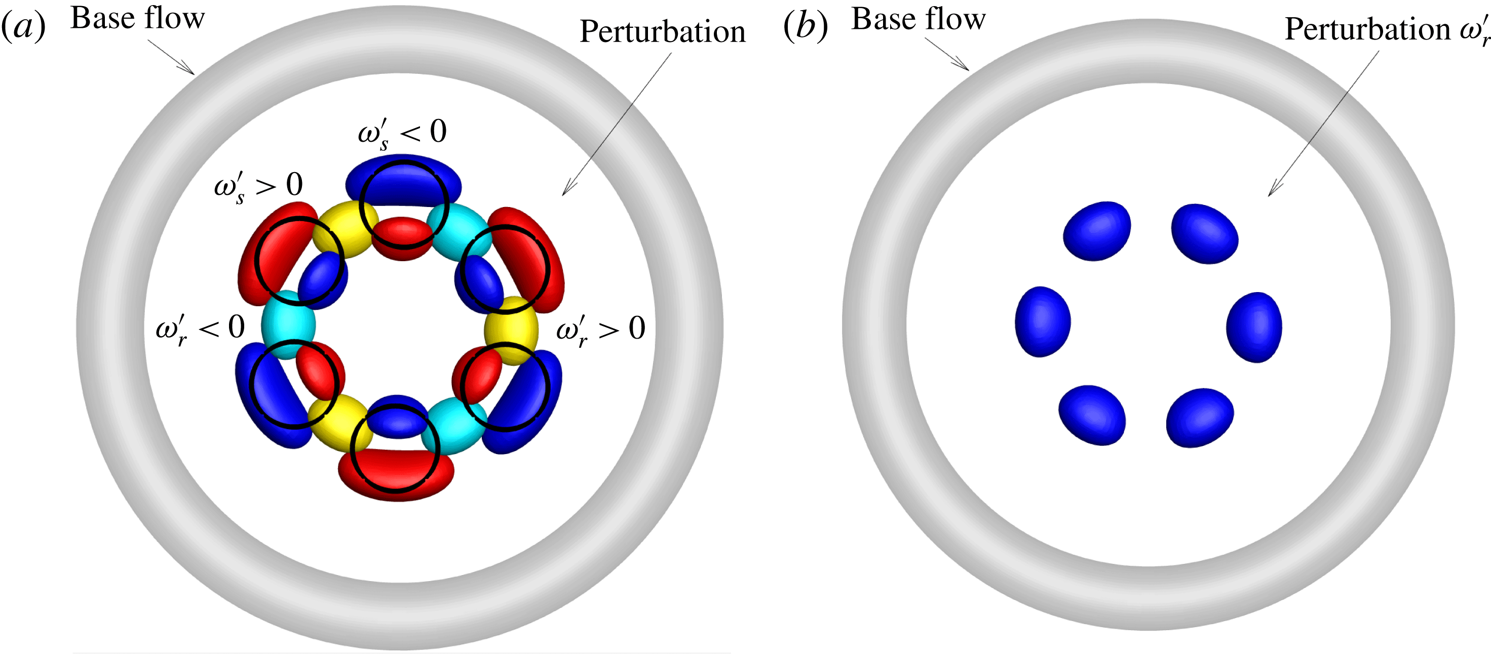
A three-dimensional plot of the perturbation structure is presented in figure 4(a). The black circles in figure 4(a) represent the perturbation formed ringlets that will be elaborated on in the following sections. Each ringlet can be roughly decomposed into four vorticity components: a positive and negative pair of
 $\unicode[STIX]{x1D714}_{s}^{\prime }$
, and a positive and negative pair of
 $\unicode[STIX]{x1D714}_{r}^{\prime }$
. The
 $\unicode[STIX]{x1D714}_{s}^{\prime }$
component is generated by
 $u_{\unicode[STIX]{x1D703}}^{\prime }$
and
 $u_{r}^{\prime }$
and amplified via the Orr mechanism. The
 $\unicode[STIX]{x1D714}_{r}^{\prime }$
component is amplified through a novel vorticity amplification mechanism. As proved in appendix A, for perturbations with
 $\unicode[STIX]{x1D714}_{\unicode[STIX]{x1D703}}^{\prime }\unicode[STIX]{x1D714}_{r}^{\prime }<0$
, the
 $\unicode[STIX]{x1D714}_{r}^{\prime }$
component is amplified, while for those with
 $\unicode[STIX]{x1D714}_{\unicode[STIX]{x1D703}}^{\prime }\unicode[STIX]{x1D714}_{r}^{\prime }>0$
,
 $\unicode[STIX]{x1D714}_{r}^{\prime }$
decays. As shown in figure 4, all the
 $\unicode[STIX]{x1D714}_{r}^{\prime }$
structures correspond to
 $\unicode[STIX]{x1D714}_{\unicode[STIX]{x1D703}}^{\prime }\unicode[STIX]{x1D714}_{r}^{\prime }<0$
and therefore undergo growth. As the
 $\unicode[STIX]{x1D714}_{r}^{\prime }$
component corresponds to finger structures extending from the ring centre to the core, this vorticity amplification mechanism also explains the coherent finger-like structures observed by Deng et al. (Reference Deng, Xue, Mao and Caulfield2017).
(a) Iso-surfaces of
 $\unicode[STIX]{x1D714}_{s}^{\prime }$
and
 $\unicode[STIX]{x1D714}_{r}^{\prime }$
. Red and blue represent positive and negative values of
 $\unicode[STIX]{x1D714}_{s}^{\prime }$
, respectively, and yellow and cyan denote positive and negative values of
 $\unicode[STIX]{x1D714}_{r}^{\prime }$
, respectively. (b) Iso-surfaces of
 $\unicode[STIX]{x1D714}_{r}^{\prime }$
coloured by
 $\unicode[STIX]{x1D714}_{\unicode[STIX]{x1D703}}^{\prime }\unicode[STIX]{x1D714}_{r}^{\prime }$
, with blue denoting negative values. The perturbation is evolved to
 $t=4$
from the optimal initial condition at
 $m=3$
and
 $\unicode[STIX]{x1D70F}=10$
. The base flow is in grey colour. The circles in (a) represents the ringlets that the perturbations form.
For both the Orr and vorticity-amplification mechanisms addressed above, which correspond to two- and three-dimensional perturbation amplifications, respectively, the transient growth is associated with the base flow outside the vortex core. Such growths will not occur if the vortex is compact, similar to that identified in a straight vortex flow (Pradeep & Hussain Reference Pradeep and Hussain2006).
4 DNS of the optimally perturbed ring
4.1 Nonlinear development of perturbations at various parameters
In this section, the base flow is initially perturbed by the optimal perturbation with a relative magnitude
 $k$
, which represents the square root of the ratio of the perturbation energy to the base energy integrated over the computational domain (the base energy is generated from (3.1)–(3.3) without the
 $u_{0}$
term). The linear study in the previous section can be also interpreted as the perturbation dynamics at sufficiently small
 $k$
.
 $k=6\times 10^{-3}$
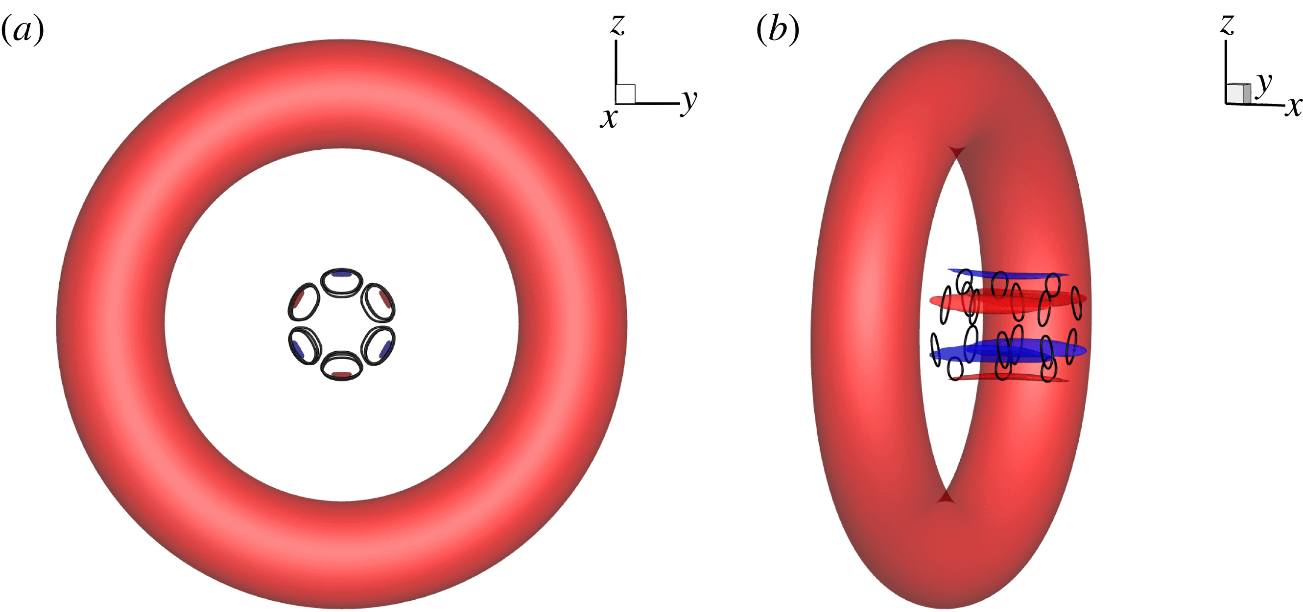
unless otherwise stated, and it corresponds to a maximum perturbation velocity 0.05. In the azimuthal direction, 128 Fourier modes are computed. The initially perturbed flow is visualised by iso-surfaces of
 $\unicode[STIX]{x1D714}_{s}$
and vortex lines (similar circular lines have been plotted in figure 4
a) in figure 5. Clearly the perturbation is concentrated on the axis of the ring, in the form of
 $2m$
(
 $m=3$
) elongated ring structures.
Top (a) and oblique (b) views of the iso-surfaces of
 $\unicode[STIX]{x1D714}_{s}$
for the initial condition in DNS. Red and blue denote
 $\unicode[STIX]{x1D714}_{s}=2$
and
 $-2$
respectively. The perturbation magnitude is
 $k=6\times 10^{-3}$
here and in the following figures unless stated. Circular lines denote vortex lines.
Iso-surfaces of
 $\unicode[STIX]{x1D706}_{2}=-0.5$
, coloured by
 $\unicode[STIX]{x1D714}_{s}$
at
 $t=4,6$
and
 $8$
from left to right. The ringlets are delineated by vortex lines (circular lines in a–f). The initial perturbation is optimal at
 $m=3$
, 5 and 11 in the top, middle and bottom rows.

The iso-surfaces of
 $\unicode[STIX]{x1D706}_{2}=-0.5$
are used to visualise the vortical structures during the nonlinear development of the optimal initial perturbation, as shown in figure 6. Here
 $\unicode[STIX]{x1D706}_{2}$
is defined as the second solution of a cubic characteristic equation and the negative value of
 $\unicode[STIX]{x1D706}_{2}$
can be used to identify a vortex (Jeong & Hussain Reference Jeong and Hussain1995). For the initial perturbation calculated at
 $m=3$
and
 $m=5$
, circular structures, which denote amplified ringlets, are observed at
 $t=6$
and these structures are wrapped around the ring at later times. Then, owing to the stretching of the base flow streamlines and the linear perturbation growth mechanisms discussed in §§ 3.3 and 3.4, these original structures are enlarged and their kinetic energy can be amplified over
 $200$
times (see figure 2) in the linear limit and over
 $100$
times in the present nonlinear case. At a later time when the perturbations are advected to the main ring via self-induction of the ringlets, the core modes, featuring a deformation of the ring core, are also activated (the right column in figure 6, albeit rather weak). Similar amplification and dynamics of ringlets are observed at other wavenumbers e.g.
 $m=1$
,
 $2$
,
 $4$
, etc. (not shown here).
At larger wavenumbers, e.g. the linearly most energetic non-zero wavenumber
 $m=11$
, the finger-like structures are significantly elongated and ringlets are not clearly observed (see the bottom row of figure 6). At this wavenumber, even in the initial condition, the core modes are activated and become dominant soon. The perturbation structures are with low values of
 $\unicode[STIX]{x1D714}_{s}^{\prime }$
as they are dominated by
 $\unicode[STIX]{x1D714}_{\unicode[STIX]{x1D703}}^{\prime }$
and
 $\unicode[STIX]{x1D714}_{r}^{\prime }$
. At
 $t=8$
, shown in figure 6(l), secondary vortical structures are formed around the original vortex core apart from the finger-like structures outside the core. These secondary structures have previously been termed as ‘halo’ vorticity and were also observed in previous DNS and experimental works (Bergdorf et al.
Reference Bergdorf, Koumoutsakos and Leonard2007; Archer et al.
Reference Archer, Thomas and Coleman2008; Sullivan et al.
Reference Sullivan, Niemela, Hershberger, Bolster and Donnelly2008). The finger-like structures are outcomes of the optimal transient energy growth, and their forms are similar to the well reported lobe structures, which however are located in the vortex core (Shadden, Dabiri & Marsden Reference Shadden, Dabiri and Marsden2006). The core of the ring is displaced into a stationary wave form, manifesting the elliptic instability, which has been well addressed in previous stability and DNS works and will not be pursued here (Archer et al.
Reference Archer, Thomas and Coleman2008).
Other perturbation magnitudes are also studied (not shown here). As expected, at higher values of the initial perturbation amplitude
 $k$
, the ringlets become stronger and are increasingly separated into two layers owing to the nonlinear perturbation-induced effect. These observations demonstrate that the generation of ringlets induced by transient energy growth is robust, across various perturbation amplitudes and spanwise wavenumbers. It will be further presented in § 4.4 that the perturbation growth and the generation of ringlets addressed above can be also observed in a randomly perturbed ring. This is because the optimal initial perturbation is the most amplified component of a random disturbance and will manifest itself over a transient period. In the following, the mechanism of the ringlet generation is analysed.
4.2 Mechanisms of amplification of ringlets
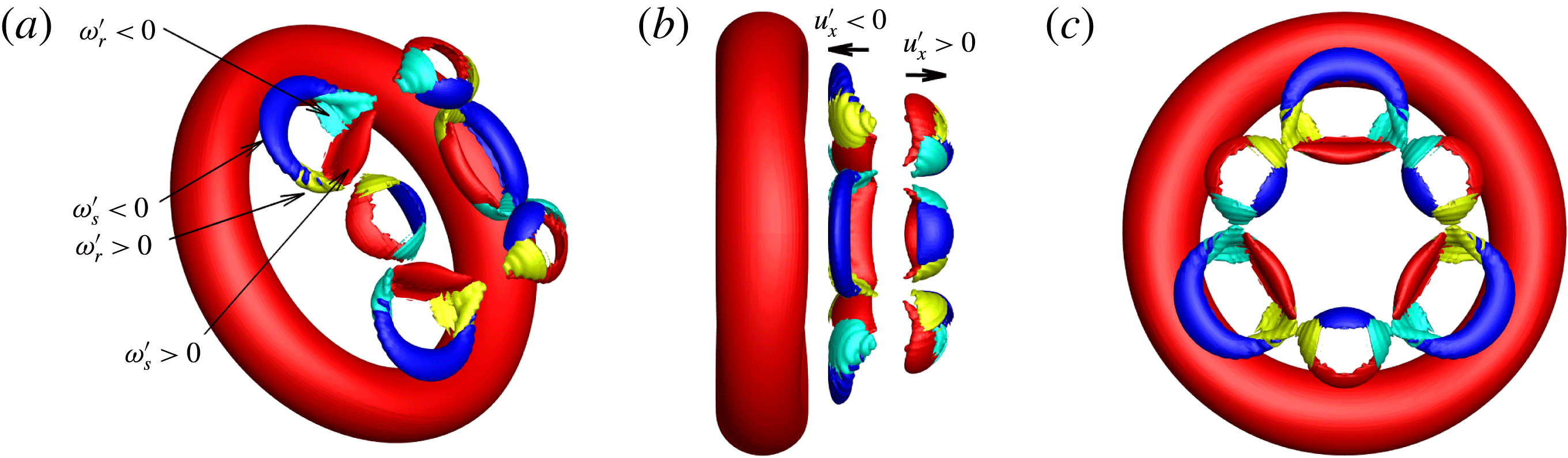
In this section, the vorticity components of the ringlets are decomposed to analyse their generation. As can be inferred from the location of the ringlets and also shown in figure 7, each ringlet consists of four parts: positive and negative
 $\unicode[STIX]{x1D714}_{s}^{\prime }$
, and positive and negative
 $\unicode[STIX]{x1D714}_{r}^{\prime }$
. In the linear analyses, we showed that
 $\unicode[STIX]{x1D714}_{s}^{\prime }$
and
 $\unicode[STIX]{x1D714}_{r}^{\prime }$
can be generated and amplified by the Orr and vorticity-amplification mechanisms, respectively. In figures 4 and 5, there are six such combinations around the axis of the ring. Examining the perturbation-induced velocity in the
 $x$
direction, we see that three of them are with
 $u_{x}^{\prime }<0$
while the other three with
 $u_{x}^{\prime }>0$
. This induced velocity then drives three ringlets away from the ring and the other three towards the ring, resulting in two layers of ringlet structures. The layer closer to the ring is stretched and enlarged by the velocity field of the main ring.
(a–c): Oblique, side and top views of iso-surfaces of vorticity at
 $t=4$
, respectively. Each ringlet can be decomposed to four vorticity segments: positive and negative values of
 $\unicode[STIX]{x1D714}_{s}$
denoted by red and blue, respectively; positive and negative values of
 $\unicode[STIX]{x1D714}_{r}$
represented by yellow and cyan, respectively. The arrows in (b) denote the direction of the self-induced motion.
Starting from the optimal initial perturbation with azimuthal wavenumber
 $m=3$
, as shown in figures 3 and 5, the mechanisms of the vortex ring generation can be summarised as follows.
-
(i) The perturbation exhibiting
 $u_{r}^{\prime }u_{\unicode[STIX]{x1D703}}^{\prime }>0$
is tilted forward by the base flow as presented in figure 3. In this process
$\unicode[STIX]{x1D714}_{s}^{\prime }$
is amplified through an Orr mechanism. The
$\unicode[STIX]{x1D714}_{r}^{\prime }$
component is amplified via a novel vorticity-amplification mechanism.
-
(ii) When the perturbation amplitude is not small enough, it will be driven by its own component to separate into two layers (see figure 7 b).
-
(iii) As one layer is advected away from the main ring, the other layer closer to the ring is stretched and enlarged by the base flow streamlines. The
$\unicode[STIX]{x1D714}_{s}^{\prime }$
and
$\unicode[STIX]{x1D714}_{r}^{\prime }$
components form ringlet structures.


Schematic of the perturbation development. The red circle denotes the base ring and the red arrows represent the base velocity.
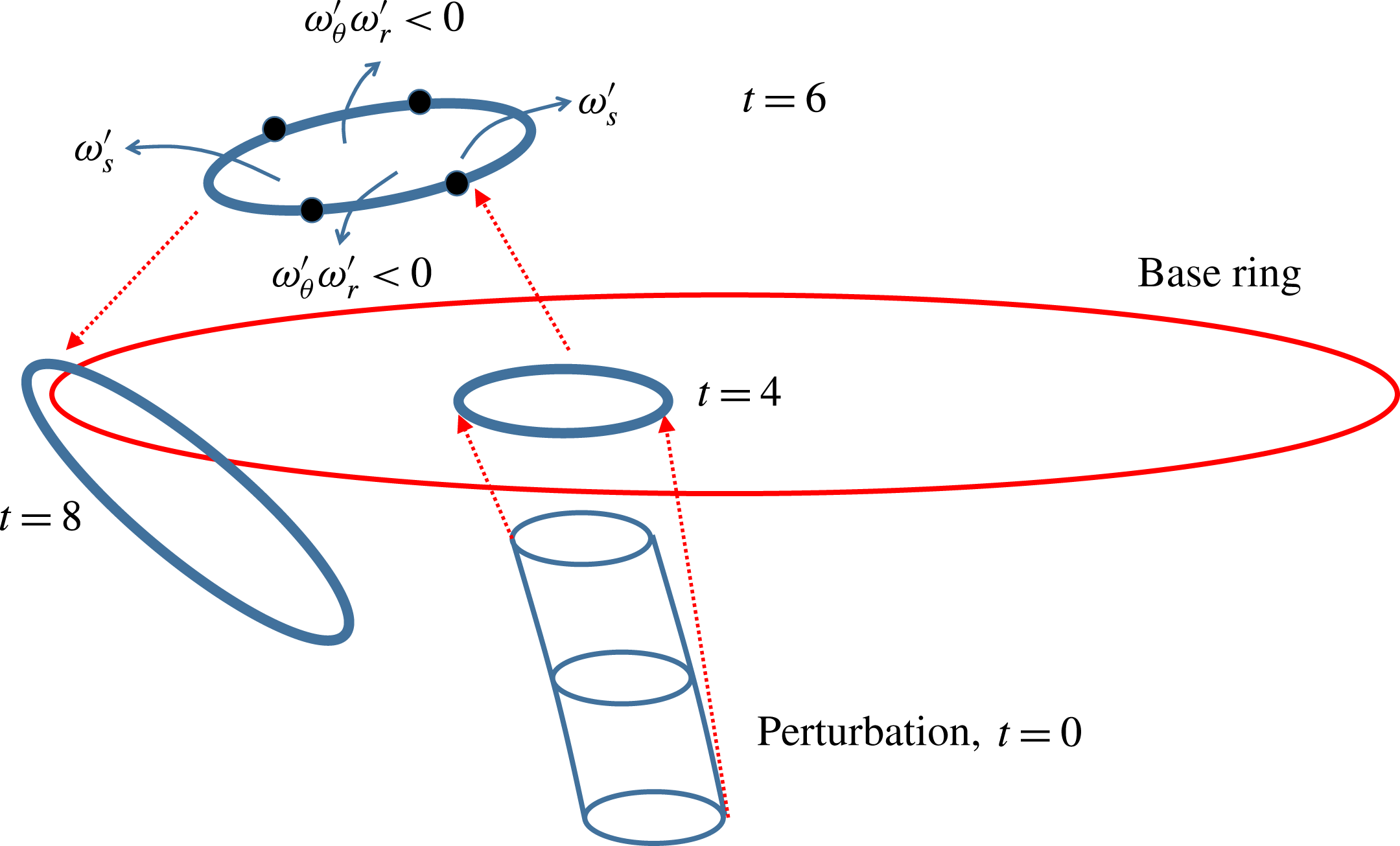
The development of optimal perturbations is schematically plotted in figure 8. From the vorticity of the ringlet, four segments can be identified as presented above and also by the blue arrow streamlines in figure 8. Two segments correspond to
 $\unicode[STIX]{x1D714}_{s}^{\prime }$
with
 $u_{\unicode[STIX]{x1D703}}^{\prime }u_{r}^{\prime }>0$
(see figure 3), while the other two are dominated by
 $\unicode[STIX]{x1D714}_{\unicode[STIX]{x1D703}}^{\prime }$
and
 $\unicode[STIX]{x1D714}_{r}^{\prime }$
with
 $\unicode[STIX]{x1D714}_{\unicode[STIX]{x1D703}}^{\prime }\unicode[STIX]{x1D714}_{r}^{\prime }<0$
(see figure 4). Therefore the first two segments are amplified by the Orr mechanism and the other two by the vorticity-amplification mechanism. After the linear growth, the ringlets are further stretched by the base ring and wrapped around it. It will be shown in the next section that at a higher Reynolds number, this process induces a new mode of breakup of the base ring.
4.3 Cascade of ringlets at higher Reynolds number
The Reynolds number
 $Re=10\,000$
in all the above studies. As ringlets are the most amplified structures by a larger ring, it can be anticipated that at higher Reynolds number, the secondary ringlets will trigger a tertiary group of ringlets.
 $Re=27\,000$
is then simulated to examine this possible cascade of ring structures. As the initial perturbation has azimuthal wavenumber
 $m=3$
, modes with
 $m=3N$
(
 $N$
is an integer number) can be generated by nonlinear interactions, and other modes (e.g.
 $m=1$
,
 $2$
) can only be activated by round-off error. Therefore only
 $1/3$
of the domain is considered.
 $200$
Fourier modes are computed with azimuthal wavenumbers
 $3N$
(
 $N=0,1,\ldots ,199$
).
(a–d) Iso-surfaces of
 $\unicode[STIX]{x1D714}_{s}=3$
at
 $Re=27\,000$
and time
 $t=0,4,6$
and
 $8$
, respectively. Circular lines denote vortex lines.

The results are then repeated twice in the azimuthal direction to recover the full domain, as shown in figure 9. Vortex lines are used to highlight the development of ringlets. The base ring is denoted as ‘A’ and can be identified by both iso-surfaces of
 $\unicode[STIX]{x1D714}_{s}$
and vortex lines. At
 $t=0$
, the perturbations are concentrated around the ring axis and are in the form of two groups of ringlets, denoted as ‘B’ and ‘C’. At
 $t=4$
, these two groups are amplified, enlarged and detached to form two layers in the streamwise direction (as shown in figure 7
b at a lower
 $Re$
). At
 $t=6$
, another group of even smaller ringlets, denoted as ‘D’, appears. This group is amplified by ringlets ‘B’ through transient perturbation growth, since rings are the most amplified structures in a ring flow as illustrated in figure 5. Therefore the transient growth induces a cascade of ringlets: group ‘A’ amplifies group ‘B’ and ‘C’, and then group ‘B’ amplifies group ‘D’, and so on. As ‘B’ is not optimally perturbed but it still induces ringlets ‘D’, this observation indicates that the transient growth and the generation of ringlets exist without imposing the optimal initial perturbation. At
 $t=8$
, groups ‘B’ and ‘C’ are wrapped around the outer region of the ring, and similarly group ‘D’ is wrapped around group ‘B’. Compared with the
 $Re=10\,000$
case, we note that a larger
 $Re$
enriches the vortex dynamics and supports the generation of smaller coherent structures in the form of a cascade of ringlets.
Iso-surfaces of
 $\unicode[STIX]{x1D714}_{s}$
at
 $Re=27\,000$
and
 $t=10$
and
 $12$
for (a) and (b), respectively. Blue, cyan, yellow and red colours represent
 $\unicode[STIX]{x1D714}_{s}=-10,-5,5$
and
 $10$
in (a), and
 $\unicode[STIX]{x1D714}_{s}=-16,-8,8$
and
 $16$
in (b). Circular lines denote vortex lines.

A further development of the perturbed ring is shown in figure 10. As the perturbation has a dominant wavenumber
 $m=3$
, the main ring ‘A’ presents a triangular vortex line at
 $t=10$
(see figure 10
a). The group ‘B’ has merged with ‘A’ and becomes the dominant structure (with the largest magnitude of
 $\unicode[STIX]{x1D714}_{s}$
), whilst groups ‘C’ and ‘D’ are distorted when wrapped around ‘A’. Note that vortical structures with a larger radius than the main ring are generated and they present the inviscid helical instabilities that were widely observed in straight vortices with an axial flow (Lessen, Singh & Paillet Reference Lessen, Singh and Paillet1974). At later times, a turbulent ring is observed (see figure 10
b). The disturbance has effectively broken the core of the ring into three sections whereas the ringlets are no longer observable. The helical vortices with a larger radius than the ring observed at
 $t=10$
have broken to several segments. While these observations indicate that the ringlets are transient, a new ringlet grows from the centre of the ring. The breakup of this ring is dramatically different from the scenario of breakup driven by smaller-scale structures, e.g. core instabilities or the ‘halo’ structures observed in previous DNS studies.
4.4 Cascade of ringlets in a randomly perturbed ring
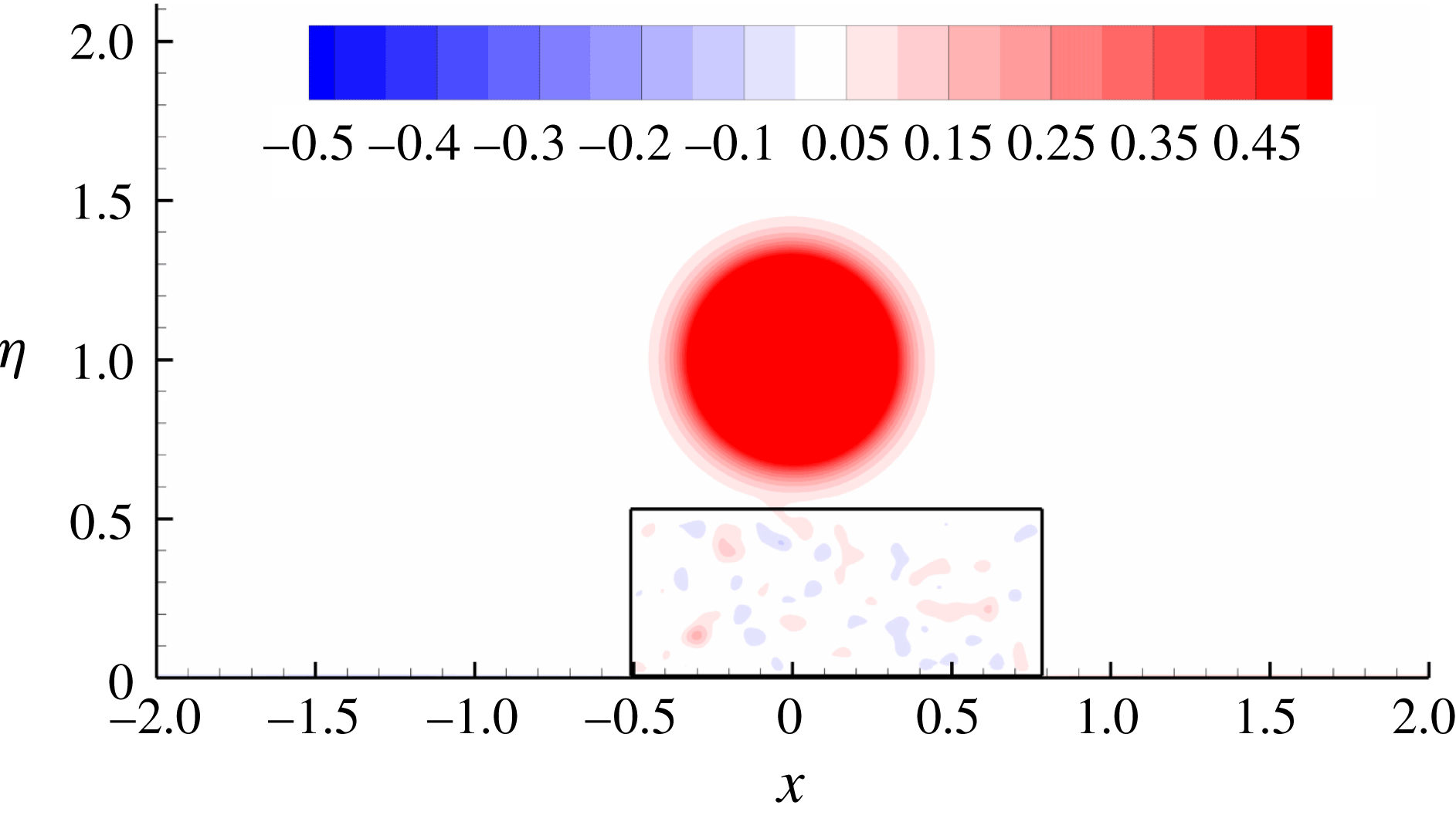
All the DNS studies conducted above adopted the linearly optimal initial perturbation. To demonstrate the linear transient growth and nonlinear dynamics in real conditions, a random perturbation with a maximum velocity magnitude 0.04 is projected onto the divergence-free space and then used as the initial disturbance. As perturbations located around the core activate core instabilities, the random perturbation is only introduced in the axial region, enclosed by black lines in figure 11. Similarly as in § 4.3, one third of the domain is considered and therefore the random disturbance and its induced outcome have an azimuthal wavenumber
 $m=3$
.
Contours of
 $\unicode[STIX]{x1D714}_{s}$
in a vortex ring perturbed by random initial disturbance at
 $Re=27\,000$
. The black lines enclose a box where the disturbance is introduced.
Iso-surfaces of
 $\unicode[STIX]{x1D714}_{s}$
at
 $Re=27\,000$
in the randomly perturbed ring. (a) Side view at
 $t=6$
, and (b), (c) and (d) top views at
 $t=6$
,
 $10$
and
 $12$
respectively. Blue, cyan, yellow and red colours represent
 $\unicode[STIX]{x1D714}_{s}=-10,-5,5$
and
 $10$
in (a), (b) and (c), and
 $\unicode[STIX]{x1D714}_{s}=-16,-8,8$
and
 $16$
in (d). Circular lines denote vortex lines.

Then this randomly perturbed ring is evolved via DNS. At
 $t=6$
(see figure 12
a and b), the three groups of rings can be clearly observed as in the optimally perturbed case. ‘A’ denotes the original ring, while ‘B’ and ‘C’ are ringlets induced by transient growth of perturbations. Due to the self-induced velocity, group ‘B’ is closer to ‘A’, and is stretched to the core of ‘A’. At later times shown in figure 12(c) and (d), the vortical structures induced by ringlets ‘B’ become dominant and lead to the breakup of the core of the main ring as seen in the optimally perturbed case.
5 Conclusion
While prior works on the dynamics of vortex rings focused on the core region, the present work instead addresses the near-axis region of the ring. Elongated ringlet structures are the most amplified through transient growth. Such a growth associated with the base flow outside the vortex core has been well observed in straight vortex flows (Mao & Sherwin Reference Mao and Sherwin2012; Stout & Hussain Reference Stout and Hussain2016).
The most energetic perturbations are calculated at Reynolds numbers
 $Re=10\,000$
and
 $Re=27\,000$
. The optimal perturbation then evolves into three-dimensional coherent structures. At azimuthal wavenumber
 $m=11$
, which corresponds to a local peak of transient growth, the optimal perturbation develops into finger-like structures outside the vortex core. The modes with
 $m=5$
and
 $m=3$
induce ringlets owing to the combination of the Orr mechanism, a unique inviscid vorticity amplification mechanism and an induced axial velocity. The generation of these ringlets is robust: they are observed at various initial perturbation amplitudes, azimuthal wavenumbers and values of
 $Re$
, as well as in a randomly perturbed ring flow.
At
 $Re=27\,000$
, the secondary ringlets amplified by the primary ring induce a tertiary group of even smaller ringlets through similar transient perturbation growth. This cascade of ring structures indicates that the mechanism of amplification of ringlets by a base ring is universal and does not rely on a subtly selected initial perturbation. A further nonlinear development of the ringlets induces a novel mode of breakup of the main ring, in contrast to the well addressed core breakup.
Compared with most previous works on the core dynamics and turbulent structures, the present work focuses on ringlets, stemming from perturbations around the ring axis. The novel mechanism of ring generation and the mode of ring breakup are likely to have significant roles in many vortex ring flows, particularly in the case that a control forcing cannot be introduced in the core region. For example, in a synthetic jet flow, if the centre of the ring is perturbed, the generated ringlets would accelerate transition and enhance the control effects (Jabbal & Zhong Reference Jabbal and Zhong2010); in combustion, these rings would enhance mixing and efficient combustion; in jet flow, these ringlets are asymmetric with respect to the axis of the main ring and will affect production of jet noise (Bridges & Hussain Reference Bridges and Hussain1992); in a helicopter, the axial perturbation can be generated from the hub of the rotor to mitigate the detrimental vortex ring state in a descending motion.
Acknowledgements
This work was supported by the Engineering and Physical Sciences Research Council [grant number EP/M025039/2].
Appendix A. Mechanism of inviscid vorticity amplification
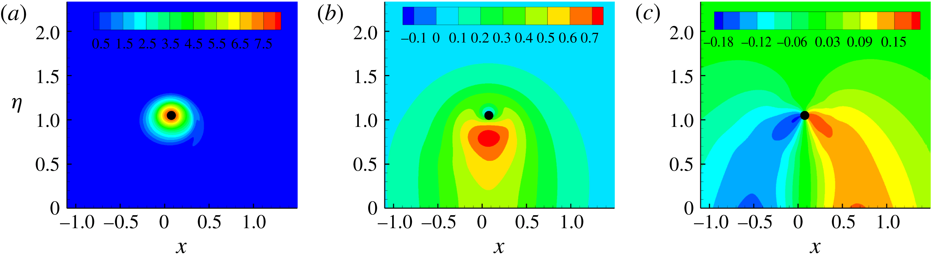
The base flow is illustrated in figure 13. The azimuthal vorticity is concentrated around the core and decays to negligible levels around the ring axis (
 $x$
axis). Since the vortex profile in the
 $x{-}\unicode[STIX]{x1D702}$
plane is distorted,
 $\unicode[STIX]{x2202}_{\unicode[STIX]{x1D703}}u_{\unicode[STIX]{x1D703}}$
and
 $\unicode[STIX]{x2202}_{r}u_{r}$
have non-zero values.
Contours of (a)
 $\bar{\unicode[STIX]{x1D714}}_{s}$
, (b)
 $\bar{u}_{\unicode[STIX]{x1D703}}$
and (c)
 $\bar{u}_{r}$
in the base flow at
 $t=4$
. Since the flow is homogeneous in
 $\unicode[STIX]{x1D719}$
, two-dimensional plots in an
 $x{-}\unicode[STIX]{x1D702}$
plane are adopted. The filled black circle represents the origin of the
 $(s,r,\unicode[STIX]{x1D703})$
system (marked as
 $c$
in figure 1).
Start from the vorticity equation:
 $$\begin{eqnarray}{\displaystyle \frac{\text{D}\unicode[STIX]{x1D74E}}{\text{D}t}}=\unicode[STIX]{x1D74E}\boldsymbol{\cdot }\unicode[STIX]{x1D735}\boldsymbol{u}+Re^{-1}\unicode[STIX]{x1D6FB}^{2}\boldsymbol{u},\end{eqnarray}$$
where
 $\unicode[STIX]{x1D74E}$
denotes the vorticity vector and
 $\text{D}/\text{D}t$
is the material derivative.
Decomposing the flow into a base component
 $(\bar{\unicode[STIX]{x1D74E}},\bar{\boldsymbol{u}})$
and a perturbation component
 $(\unicode[STIX]{x1D74E}^{\prime },\boldsymbol{u}^{\prime })$
, and neglecting the nonlinear term and viscous diffusion, there is
 $$\begin{eqnarray}{\displaystyle \frac{\text{D}\unicode[STIX]{x1D74E}^{\prime }}{\text{D}t}}=\bar{\unicode[STIX]{x1D74E}}\boldsymbol{\cdot }\unicode[STIX]{x1D735}\boldsymbol{u}^{\prime }+\unicode[STIX]{x1D74E}^{\prime }\boldsymbol{\cdot }\unicode[STIX]{x1D735}\bar{\boldsymbol{u}}.\end{eqnarray}$$
In the system
 $(s,r,\unicode[STIX]{x1D703})$
,
 $\unicode[STIX]{x1D74E}=(\unicode[STIX]{x1D714}_{s},\unicode[STIX]{x1D714}_{r},\unicode[STIX]{x1D714}_{\unicode[STIX]{x1D703}})^{\text{T}}$
,
 $\boldsymbol{u}=(u_{s},u_{r},u_{\unicode[STIX]{x1D703}})^{\text{T}}$
,
 $\bar{\unicode[STIX]{x1D74E}}=(\bar{\unicode[STIX]{x1D714}}_{s},\bar{\unicode[STIX]{x1D714}}_{r},\bar{\unicode[STIX]{x1D714}}_{\unicode[STIX]{x1D703}})^{\text{T}}$
,
 $\unicode[STIX]{x1D74E}^{\prime }=(\unicode[STIX]{x1D714}_{s}^{\prime },\unicode[STIX]{x1D714}_{r}^{\prime },\unicode[STIX]{x1D714}_{\unicode[STIX]{x1D703}}^{\prime })^{\text{T}}$
,
 $\bar{\boldsymbol{u}}=(\bar{u}_{s},\bar{u}_{r},\bar{u}_{\unicode[STIX]{x1D703}})^{\text{T}}$
and
 $\boldsymbol{u}^{\prime }=(u_{s}^{\prime },u_{r}^{\prime },u_{\unicode[STIX]{x1D703}}^{\prime })^{\text{T}}$
. The two terms on the left-hand side of (A 2) can be expressed as
 $$\begin{eqnarray}\bar{\unicode[STIX]{x1D74E}}\boldsymbol{\cdot }\unicode[STIX]{x1D735}\boldsymbol{u}^{\prime }=\left(\begin{array}{@{}c@{}}{\displaystyle \frac{\bar{\unicode[STIX]{x1D714}}_{s}}{h_{s}}}\unicode[STIX]{x2202}_{s}u_{s}^{\prime }+\bar{\unicode[STIX]{x1D714}}_{r}\unicode[STIX]{x2202}_{r}u_{s}^{\prime }+{\displaystyle \frac{\bar{\unicode[STIX]{x1D714}}_{\unicode[STIX]{x1D703}}}{r}}\unicode[STIX]{x2202}_{\unicode[STIX]{x1D703}}u_{s}^{\prime }+{\displaystyle \frac{\unicode[STIX]{x1D716}(\bar{\unicode[STIX]{x1D714}}_{r}\sin \unicode[STIX]{x1D703}+\bar{\unicode[STIX]{x1D714}}_{\unicode[STIX]{x1D703}}\cos \unicode[STIX]{x1D703})}{h_{s}}}u_{s}^{\prime }\\ {\displaystyle \frac{\bar{\unicode[STIX]{x1D714}}_{s}}{h_{s}}}\unicode[STIX]{x2202}_{s}u_{r}^{\prime }+\bar{\unicode[STIX]{x1D714}}_{r}\unicode[STIX]{x2202}_{r}u_{r}^{\prime }+{\displaystyle \frac{\bar{\unicode[STIX]{x1D714}}_{\unicode[STIX]{x1D703}}}{r}}\unicode[STIX]{x2202}_{\unicode[STIX]{x1D703}}u_{r}^{\prime }-{\displaystyle \frac{\bar{\unicode[STIX]{x1D714}}_{\unicode[STIX]{x1D703}}}{r}}u_{\unicode[STIX]{x1D703}}^{\prime }-{\displaystyle \frac{\unicode[STIX]{x1D716}\bar{\unicode[STIX]{x1D714}}_{s}\sin \unicode[STIX]{x1D703}}{h_{s}}}u_{s}^{\prime }\\ {\displaystyle \frac{\bar{\unicode[STIX]{x1D714}}_{s}}{h_{s}}}\unicode[STIX]{x2202}_{s}u_{\unicode[STIX]{x1D703}}^{\prime }+\bar{\unicode[STIX]{x1D714}}_{r}\unicode[STIX]{x2202}_{r}u_{\unicode[STIX]{x1D703}}^{\prime }+{\displaystyle \frac{\bar{\unicode[STIX]{x1D714}}_{\unicode[STIX]{x1D703}}}{r}}\unicode[STIX]{x2202}_{\unicode[STIX]{x1D703}}u_{\unicode[STIX]{x1D703}}^{\prime }+{\displaystyle \frac{\bar{\unicode[STIX]{x1D714}}_{\unicode[STIX]{x1D703}}}{r}}u_{r}^{\prime }-{\displaystyle \frac{\unicode[STIX]{x1D716}\bar{\unicode[STIX]{x1D714}}_{s}\cos \unicode[STIX]{x1D703}}{h_{s}}}u_{s}^{\prime }\end{array}\right)\end{eqnarray}$$
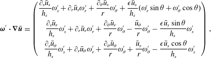 $$\begin{eqnarray}\unicode[STIX]{x1D74E}^{\prime }\boldsymbol{\cdot }\unicode[STIX]{x1D735}\bar{\boldsymbol{u}}=\left(\begin{array}{@{}c@{}}{\displaystyle \frac{\unicode[STIX]{x2202}_{s}\bar{u}_{s}}{h_{s}}}\unicode[STIX]{x1D714}_{s}^{\prime }+\unicode[STIX]{x2202}_{r}\bar{u}_{s}\unicode[STIX]{x1D714}_{r}^{\prime }+{\displaystyle \frac{\unicode[STIX]{x2202}_{\unicode[STIX]{x1D703}}\bar{u}_{s}}{r}}\unicode[STIX]{x1D714}_{\unicode[STIX]{x1D703}}^{\prime }+{\displaystyle \frac{\unicode[STIX]{x1D716}\bar{u}_{s}}{h_{s}}}(\unicode[STIX]{x1D714}_{r}^{\prime }\sin \unicode[STIX]{x1D703}+\unicode[STIX]{x1D714}_{\unicode[STIX]{x1D703}}^{\prime }\cos \unicode[STIX]{x1D703})\\ {\displaystyle \frac{\unicode[STIX]{x2202}_{s}\bar{u}_{r}}{h_{s}}}\unicode[STIX]{x1D714}_{s}^{\prime }+\unicode[STIX]{x2202}_{r}\bar{u}_{r}\unicode[STIX]{x1D714}_{r}^{\prime }+{\displaystyle \frac{\unicode[STIX]{x2202}_{\unicode[STIX]{x1D703}}\bar{u}_{r}}{r}}\unicode[STIX]{x1D714}_{\unicode[STIX]{x1D703}}^{\prime }-{\displaystyle \frac{\bar{u}_{\unicode[STIX]{x1D703}}}{r}}\unicode[STIX]{x1D714}_{\unicode[STIX]{x1D703}}^{\prime }-{\displaystyle \frac{\unicode[STIX]{x1D716}\bar{u}_{s}\sin \unicode[STIX]{x1D703}}{h_{s}}}\unicode[STIX]{x1D714}_{s}^{\prime }\\ {\displaystyle \frac{\unicode[STIX]{x2202}_{s}\bar{u}_{\unicode[STIX]{x1D703}}}{h_{s}}}\unicode[STIX]{x1D714}_{s}^{\prime }+\unicode[STIX]{x2202}_{r}\bar{u}_{\unicode[STIX]{x1D703}}\unicode[STIX]{x1D714}_{r}^{\prime }+{\displaystyle \frac{\unicode[STIX]{x2202}_{\unicode[STIX]{x1D703}}\bar{u}_{\unicode[STIX]{x1D703}}}{r}}\unicode[STIX]{x1D714}_{\unicode[STIX]{x1D703}}^{\prime }+{\displaystyle \frac{\bar{u}_{r}}{r}}\unicode[STIX]{x1D714}_{\unicode[STIX]{x1D703}}^{\prime }-{\displaystyle \frac{\unicode[STIX]{x1D716}\bar{u}_{s}\cos \unicode[STIX]{x1D703}}{h_{s}}}\unicode[STIX]{x1D714}_{s}^{\prime }\end{array}\right),\end{eqnarray}$$
where
 $\unicode[STIX]{x1D716}$
denotes the ratio of the core to the vortex radii and
 $h_{s}=1+\unicode[STIX]{x1D716}r\sin \unicode[STIX]{x1D703}$
(Fukumoto & Hattori Reference Fukumoto and Hattori2005).
Considering that the base flow satisfies
 $\unicode[STIX]{x2202}_{s}\bar{\unicode[STIX]{x1D74E}}=0$
,
 $\unicode[STIX]{x2202}_{s}\bar{\boldsymbol{u}}=0$
,
 $\bar{u}_{s}=0$
,
 $\bar{\unicode[STIX]{x1D714}}_{r}=0$
and
 $\bar{\unicode[STIX]{x1D714}}_{\unicode[STIX]{x1D703}}=0$
, and substituting (A 3) and (A 4) into (A 2), there is
 $$\begin{eqnarray}{\displaystyle \frac{\text{D}\unicode[STIX]{x1D74E}^{\prime }}{\text{D}t}}=\left(\begin{array}{@{}c@{}}{\displaystyle \frac{\bar{\unicode[STIX]{x1D714}}_{s}}{h_{s}}}\unicode[STIX]{x2202}_{s}u_{s}^{\prime }\\ {\displaystyle \frac{\bar{\unicode[STIX]{x1D714}}_{s}}{h_{s}}}\unicode[STIX]{x2202}_{s}u_{r}^{\prime }-{\displaystyle \frac{\unicode[STIX]{x1D716}\bar{\unicode[STIX]{x1D714}}_{s}\sin \unicode[STIX]{x1D703}}{h_{s}}}u_{s}^{\prime }+\unicode[STIX]{x2202}_{r}\bar{u}_{r}\unicode[STIX]{x1D714}_{r}^{\prime }+{\displaystyle \frac{\unicode[STIX]{x2202}_{\unicode[STIX]{x1D703}}\bar{u}_{r}}{r}}\unicode[STIX]{x1D714}_{\unicode[STIX]{x1D703}}^{\prime }-{\displaystyle \frac{\bar{u}_{\unicode[STIX]{x1D703}}}{r}}\unicode[STIX]{x1D714}_{\unicode[STIX]{x1D703}}^{\prime }\\ {\displaystyle \frac{\bar{\unicode[STIX]{x1D714}}_{s}}{h_{s}}}\unicode[STIX]{x2202}_{s}u_{\unicode[STIX]{x1D703}}^{\prime }-{\displaystyle \frac{\unicode[STIX]{x1D716}\bar{\unicode[STIX]{x1D714}}_{s}\cos \unicode[STIX]{x1D703}}{h_{s}}}u_{s}^{\prime }+\unicode[STIX]{x2202}_{r}\bar{u}_{\unicode[STIX]{x1D703}}\unicode[STIX]{x1D714}_{r}^{\prime }+{\displaystyle \frac{\unicode[STIX]{x2202}_{\unicode[STIX]{x1D703}}\bar{u}_{\unicode[STIX]{x1D703}}}{r}}\unicode[STIX]{x1D714}_{\unicode[STIX]{x1D703}}^{\prime }+{\displaystyle \frac{\bar{u}_{r}}{r}}\unicode[STIX]{x1D714}_{\unicode[STIX]{x1D703}}^{\prime }\end{array}\right).\end{eqnarray}$$
In the region where the optimal initial perturbation develops, the magnitude of
 $\bar{\unicode[STIX]{x1D714}}_{s}$
and
 $\unicode[STIX]{x2202}_{r}\bar{u}_{r}$
are small compared with the other terms (see figure 13). Therefore
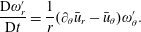 $$\begin{eqnarray}{\displaystyle \frac{\text{D}\unicode[STIX]{x1D714}_{r}^{\prime }}{\text{D}t}}={\displaystyle \frac{1}{r}}(\unicode[STIX]{x2202}_{\unicode[STIX]{x1D703}}\bar{u}_{r}-\bar{u}_{\unicode[STIX]{x1D703}})\unicode[STIX]{x1D714}_{\unicode[STIX]{x1D703}}^{\prime }.\end{eqnarray}$$
In the region the optimal perturbation develops there are
 $\unicode[STIX]{x2202}_{\unicode[STIX]{x1D703}}\bar{u}_{r}<0$
and
 $\bar{u}_{\unicode[STIX]{x1D703}}>0$
(see figure 13). Therefore if
 $\unicode[STIX]{x1D714}_{r}^{\prime }\unicode[STIX]{x1D714}_{\unicode[STIX]{x1D703}}^{\prime }>0$
, the magnitude of
 $\unicode[STIX]{x1D714}_{r}^{\prime }$
decreases, and if
 $\unicode[STIX]{x1D714}_{r}^{\prime }\unicode[STIX]{x1D714}_{\unicode[STIX]{x1D703}}^{\prime }<0$
, the
 $\unicode[STIX]{x1D714}_{r}^{\prime }$
component is amplified.


 Open access

