1 Introduction
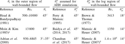
The turbulent boundary layer (TBL) consists of an ensemble of coherent motions (Robinson Reference Robinson1991) which are responsible for the production and dissipation of turbulence. Previous studies have found the majority of these motions to be inclined forwards in the direction of the mean flow. Table 1 lists a small selection of the many studies that have reported the streamwise inclination angle (
 $\unicode[STIX]{x1D703}$
) of these motions in a zero pressure gradient (ZPG) TBL at various Reynolds numbers. As is evident from the table, the value of
 $\unicode[STIX]{x1D703}$
varies significantly depending on the type of structure it is defined for, with subscripts ‘
 $m$
’ and ‘
 $s$
’ referring to inclination angle of a mean and individual flow structure, respectively (terminology inspired from Adrian, Meinhart & Tomkins (Reference Adrian, Meinhart and Tomkins2000), who also noted this difference). The superscript ‘
 $w$
’ is considered when referring to wall-attached structures only. Throughout this article, the words ‘motions’, ‘structures’ and ‘eddies’ are used interchangeably, and essentially follow the definition of a coherent motion given by Robinson (Reference Robinson1991).
A summary of the streamwise inclination angles (
 $\unicode[STIX]{x1D703}$
) of coherent motions in a ZPG TBL, estimated (
 $\unicode[STIX]{x1D703}_{s}$
,
 $\unicode[STIX]{x1D703}_{m}^{w}$
) or assumed (
 $\unicode[STIX]{x1D703}_{s}^{w}$
) in various studies. Friction Reynolds number,
 $Re_{\unicode[STIX]{x1D70F}}$
, is defined based on friction velocity (
 $u_{\unicode[STIX]{x1D70F}}$
) and TBL thickness (
 $\unicode[STIX]{x1D6FF}$
), whereas
 $Re_{\unicode[STIX]{x1D703}}$
is based on free-stream velocity (
 $U_{\infty }$
) and momentum thickness (
 $\unicode[STIX]{x1D703}$
). Terminology for angles has been described in § 1.

a This study was for a fully developed turbulent channel flow and their Reynolds number is defined based on channel centreline velocity and half-width.
b Results are for atmospheric surface layer under neutrally buoyant conditions.
The information on the structure inclination angle is important from a wall-turbulence modeller’s perspective, be it developing a model of the near-wall region for a large eddy simulation (LES; Piomelli & Balaras Reference Piomelli and Balaras2002) or to predict the TBL velocity statistics by modelling the flow based on the attached eddy hypothesis (AEH; Marusic & Monty Reference Marusic and Monty2019). The latter approach has gained popularity for investigating the kinematics in the logarithmic (log) region of a TBL by representing it with an assemblage of self-similar wall-attached vortex structures. Researchers who have utilized the AEH approach previously (table 1) assumed
 $\unicode[STIX]{x1D703}_{s}^{w}$
for these statistically representative structures to be equivalent to
 $\unicode[STIX]{x1D703}_{s}$
recorded by identifying structures via flow visualization, vortex identification techniques, and so on. Here
 $\unicode[STIX]{x1D703}_{s}$
estimated in these studies, however, was based on structures clearly discernible only in the outer region of the boundary layer (Moin & Kim Reference Moin and Kim1985), with no evidence of these being wall-coherent (hence not referred here as
 $\unicode[STIX]{x1D703}_{s}^{w}$
). Notwithstanding, the AEH simulations yield results consistent with experimental observations, suggesting
 $\unicode[STIX]{x1D703}_{s}^{w}\approx 45^{\circ }$
is a good assumption. Theoretical support towards
 $\unicode[STIX]{x1D703}_{s}^{w}$
being nominally
 $45^{\circ }$
is obtained on investigating the mean-strain-rate and rotation tensor, the two components of the velocity gradient tensor, for a ZPG TBL which is two-dimensional in the mean. As pointed out by Moin & Kim (Reference Moin and Kim1985) and Perry, Uddin & Marusic (Reference Perry, Uddin and Marusic1992), it is more likely for eddies in such a flow to assume the direction of the principal rate of mean strain since the rotation field has no preferred direction. If we consider
 $\unicode[STIX]{x1D713}$
to correspond to the inclination of the principal rate of mean strain with the streamwise direction (
 $x$
) and
 $z$
to be the wall-normal direction, it was deduced by Perry et al. (Reference Perry, Uddin and Marusic1992) that
 $$\begin{eqnarray}\unicode[STIX]{x1D713}=\frac{1}{2}\text{atan}\left(\frac{{\displaystyle \frac{\unicode[STIX]{x2202}U}{\unicode[STIX]{x2202}z}}}{2{\displaystyle \frac{\unicode[STIX]{x2202}U}{\unicode[STIX]{x2202}x}}}\right),\end{eqnarray}$$
from which
 $\unicode[STIX]{x1D713}=45^{\circ }$
for a ZPG TBL, where
 $\unicode[STIX]{x2202}U/\unicode[STIX]{x2202}x=0$
, with
 $U$
being the mean streamwise velocity. In spite of these arguments, there is still a lack of empirical evidence to support the claim of
 $\unicode[STIX]{x1D703}_{s}^{w}\approx 45^{\circ }$
.
Apart from direct visualization of individual structures, experimentalists (table 1) have statistically estimated the inclination angle of a mean wall-attached structure (
 $\unicode[STIX]{x1D703}_{m}^{w}$
) in the log region via cross-correlating simultaneously acquired wall shear stress (
 $\unicode[STIX]{x1D70F}$
) and velocity (
 $u$
) fluctuations. This is achieved through probes on the wall (
 $z=0$
) and in the log region (
 $z=z_{o}$
), respectively following
 $$\begin{eqnarray}R_{\unicode[STIX]{x1D70F}u}(\unicode[STIX]{x0394}t)=\frac{\langle \unicode[STIX]{x1D70F}(t)u(z_{o};t+\unicode[STIX]{x0394}t)\rangle }{\sqrt{\langle \unicode[STIX]{x1D70F}^{2}\rangle }\sqrt{\langle u^{2}(z_{o})\rangle }},\end{eqnarray}$$
where angle brackets (
 $\langle \,\rangle$
) denote the ensemble time average, with
 $t$
being the time. Here,
 $u$
,
 $v$
and
 $w$
refer to the streamwise, spanwise and wall-normal velocity fluctuations, respectively, associated with the coordinate system
 $x$
,
 $y$
and
 $z$
. To estimate
 $\unicode[STIX]{x1D703}_{m}^{w}$
, the temporal delay (
 $\unicode[STIX]{x0394}t_{p}$
) corresponding to the peak in
 $R_{\unicode[STIX]{x1D70F}u}$
is identified (Marusic & Heuer Reference Marusic and Heuer2007) and then
 $\unicode[STIX]{x1D703}_{m}^{w}=\text{atan}(z_{o}/(\unicode[STIX]{x0394}t_{p}U_{c}))$
, where
 $U_{c}$
is the convection velocity. The stark difference between
 $\unicode[STIX]{x1D703}_{m}^{w}$
and the expected
 $\unicode[STIX]{x1D703}_{s}^{w}$
exists due to
 $\unicode[STIX]{x1D703}_{m}^{w}$
being a function of the distribution and the range of scales of eddies convecting past the two probes (Marusic Reference Marusic2001); hence, giving it the name of a mean structure angle (figure 1 differentiates
 $\unicode[STIX]{x1D703}_{m}^{w}$
and
 $\unicode[STIX]{x1D703}_{s}^{w}$
; see also figure 13 in Head & Bandyopadhyay Reference Head and Bandyopadhyay1981). Marusic (Reference Marusic2001) demonstrated this via attached eddy simulations by considering individual eddies (with
 $\unicode[STIX]{x1D703}_{s}^{w}\approx 45^{\circ }$
) of various length scales in an organized manner, analogous to a spatially correlated packet of vortices observed experimentally by Adrian et al. (Reference Adrian, Meinhart and Tomkins2000). It was shown that
 $\unicode[STIX]{x1D703}_{m}$
, estimated from the cross-correlations obtained from these simulated fields, closely resembles the experimentally obtained inclination angles. On the other hand, it was found that
 $\unicode[STIX]{x1D703}_{m}\approx \unicode[STIX]{x1D703}_{s}$
when eddies of only specific length scales were considered in the simulation. In a real turbulent boundary layer experiment, it is possible to isolate structures of specific length scale from the rest in post-processing. In the present study, we draw inspiration from the recent work of Baidya et al. (Reference Baidya, Baars, Zimmerman, Samie, Hearst, Dogan, Mascotelli, Zheng, Bellani and Talamelli2019) to isolate large wall-attached structures in a TBL by imposing a spanwise offset between the log-region and wall probe to find
 $\unicode[STIX]{x1D703}_{s}^{w}$
.
2 Methodology adopted to isolate large wall-attached structures
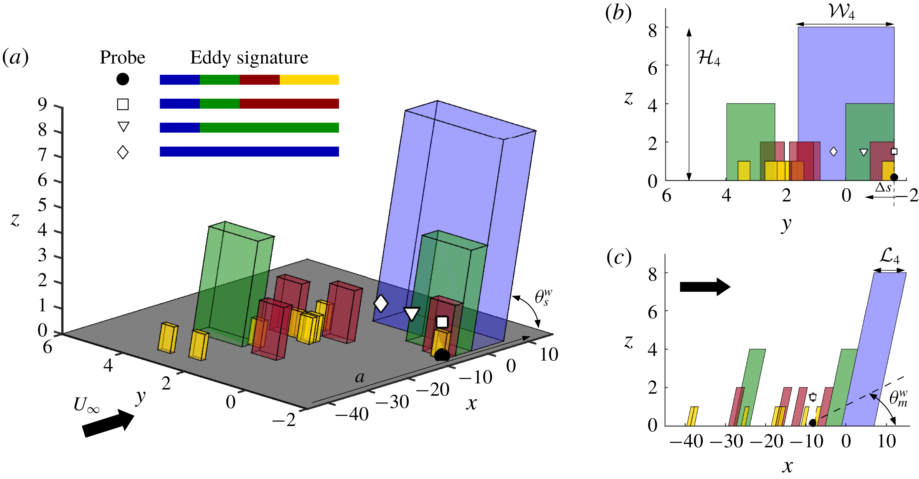
We begin by demonstrating the methodology adopted to isolate large wall-attached structures via a conceptual reconstruction of a TBL from an AEH view point. Figure 1(a–c) shows a schematic with a hierarchy of self-similar wall-attached structures representing the log region of a TBL (Baidya et al.
Reference Baidya, Baars, Zimmerman, Samie, Hearst, Dogan, Mascotelli, Zheng, Bellani and Talamelli2019; Marusic & Monty Reference Marusic and Monty2019). Apart from these preferentially forward-inclined structures, which represent the majority, a real TBL will invariably also consist of additional randomly oriented structures (Perry et al.
Reference Perry, Uddin and Marusic1992) that influence the flow statistics. These, however, are not considered in AEH-based simulations. Here, four hierarchy levels of randomly positioned attached eddies are considered, with each hierarchy shown in a different colour. Starting from the hierarchy with the smallest eddies (yellow), the eddy size in each consecutive hierarchy is doubled in a self-similar manner and the number of eddies is quartered in three-dimensional space. For simplicity, we consider the volume of influence of eddies, in each level, to be characterized by
 ${\mathcal{L}}_{i}$
,
 ${\mathcal{W}}_{i}$
and
 ${\mathcal{H}}_{i}$
in the
 $x$
,
 $y$
and
 $z$
directions, respectively, with
 $i=1$
–4 denoting the hierarchy level. A spectral analysis of the flow field consisting of such eddies would lead to their lengths and spans showing up as wavelengths,
 $\unicode[STIX]{x1D706}_{x}\sim 2{\mathcal{L}}_{i}$
and
 $\unicode[STIX]{x1D706}_{y}\sim 2{\mathcal{W}}_{i}$
(Baidya et al.
Reference Baidya, Baars, Zimmerman, Samie, Hearst, Dogan, Mascotelli, Zheng, Bellani and Talamelli2019). Here,
 $\unicode[STIX]{x1D706}_{x}=2\unicode[STIX]{x03C0}/k_{x}$
where
 $k_{x}$
is the streamwise wavenumber.
 $\unicode[STIX]{x1D703}_{s}^{w}$
represents the streamwise inclination of the individual eddies.
Schematic showing the (a) isometric, (b)
 $y$
–
 $z$
plane and (c)
 $x$
–
 $z$
plane view of a hierarchy of self-similar wall-attached eddies representing the log region of a ZPG TBL shown as simplified cuboids. Four hierarchy levels are considered, each represented by different colours. Symbols represent various probe locations. Eddy signatures identified by respective probes, over a streamwise distance of
 $a$
, are shown in (a). Here
 $L_{i}$
,
 $W_{i}$
and
 $H_{i}$
denote the streamwise, spanwise and wall-normal extent of a hierarchy level;
 $\unicode[STIX]{x1D703}_{m}^{w}$
and
 $\unicode[STIX]{x1D703}_{s}^{w}$
denote mean and individual structure angles, respectively. Figure concept adopted from Baidya et al. (Reference Baidya, Baars, Zimmerman, Samie, Hearst, Dogan, Mascotelli, Zheng, Bellani and Talamelli2019).

The solid and empty symbols represent probes placed on the wall and in the log region, respectively, to synchronously record the signature of the convecting eddies, shown in figure 1(a). The ▫ probe is able to record all except the smallest hierarchy in comparison to the wall probe (●). Accordingly, the correlation between
 $u$
fluctuations from ▫ and ● probes (following (1.2)) represents a mean structure of the wall-attached flow influenced by the hierarchy levels 2, 3 and 4 (Marusic Reference Marusic2001). The inclination angle of this mean structure is given by
 $\unicode[STIX]{x1D703}_{m}^{w}$
(figure 1
c). Increasing the relative spanwise offset (
 $\unicode[STIX]{x0394}s$
) between the log-region and wall probes means that only the hierarchy levels with the large eddies correlate between the two probes. For example, considering probe ♢ placed at
 $W_{3}<\unicode[STIX]{x0394}s<W_{4}$
, only eddies belonging to the fourth hierarchy remain correlated with the wall probe, effectively isolating these eddies from the others. Following Marusic (Reference Marusic2001), we hypothesize that the streamwise inclination angle obtained on correlating the
 $u$
fluctuations from ● and ♢ probes should reflect the angle for a large individual wall-attached structure
 $\unicode[STIX]{x1D703}_{s}^{w}$
in this simplified flow model. We consider experimental as well as numerical data sets which allow us to work along this hypothesis in the following sections. It is to be noted that the relative offset,
 $\unicode[STIX]{x0394}s$
, can be obtained on moving either the log-region or wall probe along
 $y$
, owing to the spanwise homogeneity of the TBL.
3 Experimental and numerical data
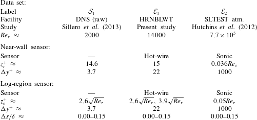
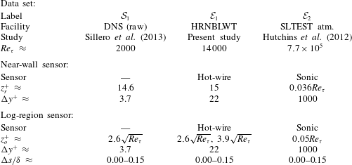
To test the hypothesis proposed in the previous section, we consider three data sets (table 2), each comprising synchronized two-point
 $u$
velocity signals at a near-wall (
 $z_{r}$
) and a log-region (
 $z_{o}$
) reference location for various spanwise offsets,
 $\unicode[STIX]{x0394}s$
. One of these is the DNS by Sillero, Jiménez & Moser (Reference Sillero, Jiménez and Moser2013) (
 ${\mathcal{S}}_{1}$
). Thirteen raw DNS time blocks, spanning up to
 $11.9\unicode[STIX]{x1D6FF}$
in
 $x$
, were considered such that the Reynolds number increases nominally across the domain. This is the same block size considered by Baars, Hutchins & Marusic (Reference Baars, Hutchins and Marusic2017) for their linear coherence spectrum (LCS) analysis with
 $Re_{\unicode[STIX]{x1D70F}}\approx 1992$
at the streamwise centre of the domain. Here, values of
 $\unicode[STIX]{x1D6FF}$
for both data sets
 ${\mathcal{S}}_{1}$
and
 ${\mathcal{E}}_{1}$
were calculated by a modified Coles law of the wake fit (Jones, Marusic & Perry Reference Jones, Marusic and Perry2001). Both
 $z_{r}^{+}$
and
 $z_{o}^{+}$
(viscous-scaled) in
 ${\mathcal{S}}_{1}$
were chosen to correspond with the experimental data set,
 ${\mathcal{E}}_{1}$
(described next).
A summary of the various data sets containing synchronized multi-point measurements at a near-wall (
 $z_{r}$
) and log-region (
 $z_{o}$
) reference location at various spanwise offsets,
 $\unicode[STIX]{x0394}s$
. Here
 $\unicode[STIX]{x0394}y^{+}$
represents the spatial resolution of the sensor/grid along the spanwise direction. DNS, direct numerical simulation; SLTEST, Surface Layer Turbulence and Environmental Science Test.
The high-
 $Re_{\unicode[STIX]{x1D70F}}$
laboratory measurements (
 ${\mathcal{E}}_{1}$
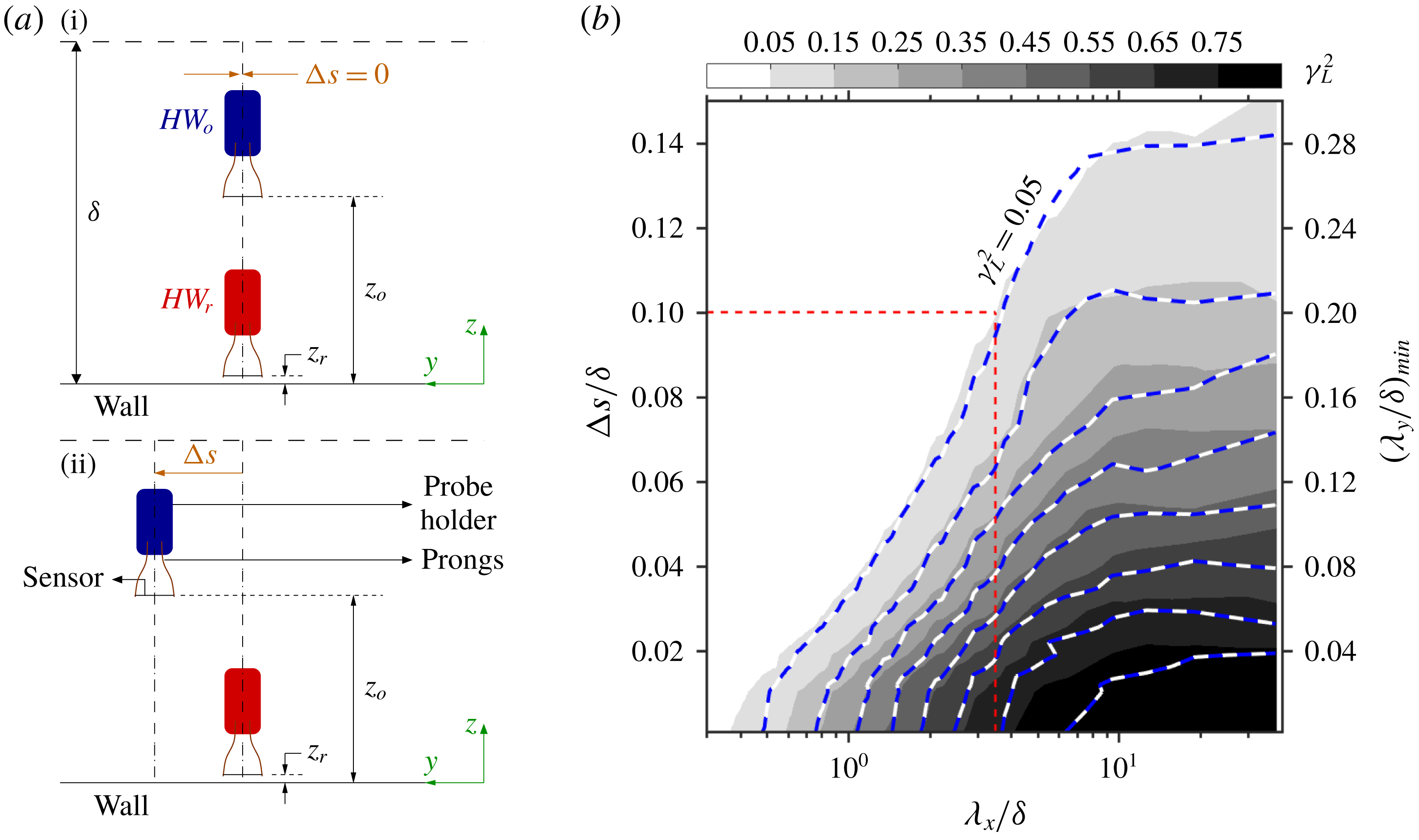
) were conducted in the large Melbourne wind tunnel (HRNBLWT). They were made possible by employing the same experimental set-up used by Chandran et al. (Reference Chandran, Baidya, Monty and Marusic2017). Figure 2(a) shows a schematic of how the experiment was conducted. The set-up comprised of two
 $2.5~\unicode[STIX]{x03BC}\text{m}$
diameter Wollaston hot-wire probes –
 $HW_{r}$
and
 $HW_{o}$
at wall-normal heights
 $z_{r}$
and
 $z_{o}$
, respectively. They were operated using an in-house Melbourne University Constant Temperature Anemometer (MUCTA) at a viscous-scaled sampling rate
 ${\sim}0.5$
. The same calibration procedure, as employed by Chandran et al. (Reference Chandran, Baidya, Monty and Marusic2017), was followed, wherein the
 $HW_{o}$
was calibrated in the TBL using the free-stream-calibrated
 $HW_{r}$
as a reference. The measurement began with both probes vertically aligned (figure 2
ai), which was ensured by viewing the arrangement via a traversable microscope. Long velocity signals were acquired with a length of
 $TU_{\infty }/\unicode[STIX]{x1D6FF}\approx 20\,000$
(
 $T$
is the total sampling duration) to obtain converged statistics at the largest energetic wavelengths. As the experiment progressed,
 $HW_{r}$
always remained at a fixed spanwise location while
 $HW_{o}$
was traversed in the spanwise direction (with log spacing) as shown in figure 2(aii).
 $HW_{o}$
was traversed only up to
 $\unicode[STIX]{x0394}s/\unicode[STIX]{x1D6FF}\approx 0.15$
since the cross-correlation tends to 0 at such spans (Baidya et al.
Reference Baidya, Baars, Zimmerman, Samie, Hearst, Dogan, Mascotelli, Zheng, Bellani and Talamelli2019). Although the present study focuses on inclination angles of wall-attached structures, a hot-wire probe positioned at
 $z_{r}^{+}\approx 15$
was preferred over a wall-mounted shear stress sensor (hot-film) owing to spatial resolution and frequency response issues (Baars et al.
Reference Baars, Hutchins and Marusic2017). This was possible due to the observation made by Baars et al. (Reference Baars, Hutchins and Marusic2017) on the wall-coherence analysis being unaffected for
 $0<z_{r}^{+}\lesssim 15$
. The data set
 ${\mathcal{E}}_{1}$
consists of two cases of
 $z_{o}^{+}$
(table 2), both lying within the log region of the TBL (Baars et al.
Reference Baars, Hutchins and Marusic2017).
(a) Schematic of the experimental set-up in HRNBLWT showing locations of the near-wall (
 $HW_{r}$
) and log-region (
 $HW_{o}$
) reference probe. Mean flow direction is along
 $x$
. The experiment begins with
 $HW_{o}$
placed vertically above
 $HW_{r}$
(
 $\unicode[STIX]{x0394}s=0$
; i) and is followed by the spanwise traverse (
 $\unicode[STIX]{x0394}s>0$
; ii) of
 $HW_{o}$
. (b)
 $\unicode[STIX]{x1D6FE}_{L}^{2}$
computed as a function of
 $\unicode[STIX]{x1D706}_{x}$
and
 $\unicode[STIX]{x0394}s$
on correlating
 $u$
from
 $HW_{o}$
and
 $HW_{r}$
for data set
 ${\mathcal{E}}_{1}$
. The grey scale and line contours correspond to
 $\unicode[STIX]{x1D6FE}_{L}^{2}$
for
 $z_{o}^{+}\approx 2.6\sqrt{Re_{\unicode[STIX]{x1D70F}}}$
and
 $3.9\sqrt{Re_{\unicode[STIX]{x1D70F}}}$
, respectively. Both contours are at levels 0.05 : 0.1 : 0.85. The red dashed line is used to highlight the streamwise spectral cutoff
 $\unicode[STIX]{x1D706}_{x,c}$
corresponding to
 $\unicode[STIX]{x0394}s/\unicode[STIX]{x1D6FF}=0.1$
.

The data set at the highest Reynolds number,
 $Re_{\unicode[STIX]{x1D70F}}\approx 7.7\times 10^{5}$
(
 ${\mathcal{E}}_{2}$
), consists of one hour of synchronously acquired
 $u$
fluctuations in the atmospheric surface layer (under near-neutral buoyant conditions) by a spanwise and wall-normal array of 18 sonic anemometers at the SLTEST facility. Here, we consider the sonic anemometers located at 4.26 m from the ground (
 $t4$
; refer figure 1 of Hutchins et al.
Reference Hutchins, Chauhan, Marusic, Monty and Klewicki2012) as the log-region reference. Of the 10 sonic anemometers in the spanwise array, each of which were separated by approximately 3 m and fixed at approximately 2.14 m from ground, we consider only four sonic anemometers (
 $s1$
–
 $s4$
) to obtain relative spanwise offsets,
 $0\lesssim \unicode[STIX]{x0394}s/\unicode[STIX]{x1D6FF}\lesssim 0.15$
(
 $\unicode[STIX]{x1D6FF}=60$
m for
 ${\mathcal{E}}_{2}$
) and to act as the near-wall reference. Given that
 $z_{r}$
is significantly far from the wall, the structure inclination angle obtained through data set
 ${\mathcal{E}}_{2}$
cannot be associated with a wall-attached structure. This data set is used here merely to demonstrate the feasibility of isolating large structures by introduction of a spanwise offset between the two reference probes. For the case of both temporal data sets
 ${\mathcal{E}}_{1}$
and
 ${\mathcal{E}}_{2}$
, Taylor’s frozen turbulence hypothesis is used to construct cross-correlation functions between
 $z_{o}$
and
 $z_{r}$
, at different streamwise (
 $\unicode[STIX]{x0394}x$
) spacings, by assuming the local mean velocity at
 $z_{o}$
(that is,
 $U(z_{o})$
) to be the convection speed (
 $U_{c}$
) of the flow structures (Baars et al.
Reference Baars, Hutchins and Marusic2017). We expect the effects due to this assumption to be minimal since the present analysis is restricted to the log region, where this assumption has been shown to perform reasonably well for estimating streamwise velocity correlations (Uddin Reference Uddin1994; de Silva et al.
Reference de Silva, Squire, Hutchins and Marusic2015). Further, as noted by Alving, Smits & Watmuff (Reference Alving, Smits and Watmuff1990), even the choice of
 $U_{c}$
does not significantly influence the estimation of the structure inclination angle.
4 Results and discussions
4.1 Variation in scale-specific wall coherence with spanwise offset
Quantitative support towards the idea of isolating large wall-attached structures in the log region (proposed in § 2) should come by analysing the one-dimensional LCS (Baars et al.
Reference Baars, Hutchins and Marusic2017; Baidya et al.
Reference Baidya, Baars, Zimmerman, Samie, Hearst, Dogan, Mascotelli, Zheng, Bellani and Talamelli2019). We employ it here to represent the streamwise-scale (
 $\unicode[STIX]{x1D706}_{x}$
) based linear coupling between
 $z_{o}$
and
 $z_{r}$
by considering
 $u$
fluctuations acquired from the probes at these two locations, for various
 $\unicode[STIX]{x0394}s$
, following
 $$\begin{eqnarray}\unicode[STIX]{x1D6FE}_{L}^{2}(z_{o},z_{r},\unicode[STIX]{x0394}s;\unicode[STIX]{x1D706}_{x})=\frac{|\langle \widetilde{u}(z_{o},\unicode[STIX]{x0394}s;\unicode[STIX]{x1D706}_{x})\widetilde{u}^{\ast }(z_{r};\unicode[STIX]{x1D706}_{x})\rangle |^{2}}{\langle |\widetilde{u}(z_{o},\unicode[STIX]{x0394}s;\unicode[STIX]{x1D706}_{x})|^{2}\rangle \langle |\widetilde{u}(z_{r};\unicode[STIX]{x1D706}_{x})|^{2}\rangle }=\frac{|{\unicode[STIX]{x1D719}_{u_{o}u_{r}}^{\prime }(z_{o},z_{r},\unicode[STIX]{x0394}s;\unicode[STIX]{x1D706}_{x})|}^{2}}{\unicode[STIX]{x1D719}_{u_{o}u_{o}}(z_{o},\unicode[STIX]{x0394}s;\unicode[STIX]{x1D706}_{x})\unicode[STIX]{x1D719}_{u_{r}u_{r}}(z_{r};\unicode[STIX]{x1D706}_{x})},\end{eqnarray}$$
where
 $\tilde{u} (z_{o},\unicode[STIX]{x0394}s;\unicode[STIX]{x1D706}_{x})={\mathcal{F}}[u(z_{o},\unicode[STIX]{x0394}s)]$
is the Fourier transform of
 $u(z_{o},\unicode[STIX]{x0394}s)$
in either time or
 $x$
depending on the data set. The asterisk (
 $\ast$
), angle brackets (
 $\langle \,\rangle$
) and vertical bars (
 $|\,|$
) indicate the complex conjugate, ensemble averaging and modulus, respectively. Thus,
 $\unicode[STIX]{x1D719}_{u_{o}u_{r}}^{\prime }$
is the one-dimensional cross-spectrum between
 $u(z_{o},\unicode[STIX]{x0394}s)$
and
 $u(z_{r})$
, while
 $\unicode[STIX]{x1D719}_{u_{o}u_{o}}$
and
 $\unicode[STIX]{x1D719}_{u_{r}u_{r}}$
are the energy spectra at
 $z_{o}$
and
 $z_{r}$
, respectively.
 $\unicode[STIX]{x1D6FE}_{L}^{2}$
may be interpreted as the spectral domain equivalent of a physical two-point correlation, and varies between
 $0\leqslant \unicode[STIX]{x1D6FE}_{L}^{2}\leqslant 1$
owing to the normalization defined in (4.1).
Figure 2(b) plots the
 $\unicode[STIX]{x1D6FE}_{L}^{2}$
contours for
 $z_{o}^{+}\approx 2.6\sqrt{Re_{\unicode[STIX]{x1D70F}}}$
and
 $3.9\sqrt{Re_{\unicode[STIX]{x1D70F}}}$
for the
 ${\mathcal{E}}_{1}$
data set. Following Baars, Hutchins & Marusic (Reference Baars, Hutchins and Marusic2016), we consider a coherence threshold of
 $\unicode[STIX]{x1D6FE}_{filt}^{2}=0.05$
to identify a streamwise spectral cutoff
 $\unicode[STIX]{x1D706}_{x,c}(z_{o},z_{r},\unicode[STIX]{x0394}s)$
to classify structures with
 $\unicode[STIX]{x1D706}_{x}>\unicode[STIX]{x1D706}_{x,c}(z_{o},z_{r},\unicode[STIX]{x0394}s)$
as being coherent between
 $z_{r}$
and
 $z_{o}$
for a specific
 $\unicode[STIX]{x0394}s$
. As discussed in § 2, it is observed that an increase in
 $\unicode[STIX]{x0394}s$
leads to reduction in the range of scales correlated between the two probes (that is, an increase in
 $\unicode[STIX]{x1D706}_{x,c}$
). While
 $\unicode[STIX]{x1D6FE}_{filt}^{2}$
is used to identify relevant streamwise wavelengths, the spanwise offset between probes inherently filters out the possible range of spanwise wavelengths (
 $\unicode[STIX]{x1D706}_{y}$
) for coherent structures; that is,
 $\unicode[STIX]{x1D706}_{y}>\unicode[STIX]{x1D706}_{y,c}$
, where
 $\unicode[STIX]{x1D706}_{y,c}/\unicode[STIX]{x1D6FF}\sim 2(\unicode[STIX]{x0394}s/\unicode[STIX]{x1D6FF})$
(this has been highlighted as
 $(\unicode[STIX]{x1D706}_{y}/\unicode[STIX]{x1D6FF})_{min}$
on the secondary
 $y$
-axis in figure 2
b). It implies that on increasing
 $\unicode[STIX]{x0394}s/\unicode[STIX]{x1D6FF}$
, for example, to 0.1, only structures with
 $\unicode[STIX]{x1D706}_{x}/\unicode[STIX]{x1D6FF}>3.5$
and
 $\unicode[STIX]{x1D706}_{y}/\unicode[STIX]{x1D6FF}>0.2$
are correlated between the two probes. This means that these wall-attached structures, which are large both in length and span, have been isolated from the remaining assemblage of eddies. Hence, the corresponding cross-correlation should not be influenced by the smaller structures.
It is noted that
 $\unicode[STIX]{x1D6FE}_{L}^{2}$
contours for the two cases of
 $z_{o}$
tend to overlap at large
 $\unicode[STIX]{x0394}s/\unicode[STIX]{x1D6FF}$
, suggesting that a similar range of large wall-attached structures (on an average) are correlated between probes at
 $z_{o}$
and
 $z_{r}$
, for any
 $z_{o}$
lying in the log region (also observed by Baidya et al.
Reference Baidya, Baars, Zimmerman, Samie, Hearst, Dogan, Mascotelli, Zheng, Bellani and Talamelli2019). Conclusions drawn from forthcoming discussions, focusing on these structures, are thus applicable across this region. Interestingly, figure 2(b) shows that superstructures (
 $\unicode[STIX]{x1D706}_{x}/\unicode[STIX]{x1D6FF}>10$
; Hutchins & Marusic Reference Hutchins and Marusic2007) remain correlated between the two probes up to
 $\unicode[STIX]{x0394}s/\unicode[STIX]{x1D6FF}\approx 0.14$
. Such large structures, however, would be absent while analysing the data set
 ${\mathcal{S}}_{1}$
due to the limited streamwise domain (
 ${\approx}11.9\unicode[STIX]{x1D6FF}$
) considered.
Cross-correlation of
 $u$
measured at
 $z_{r}$
and
 $z_{o}$
, for various
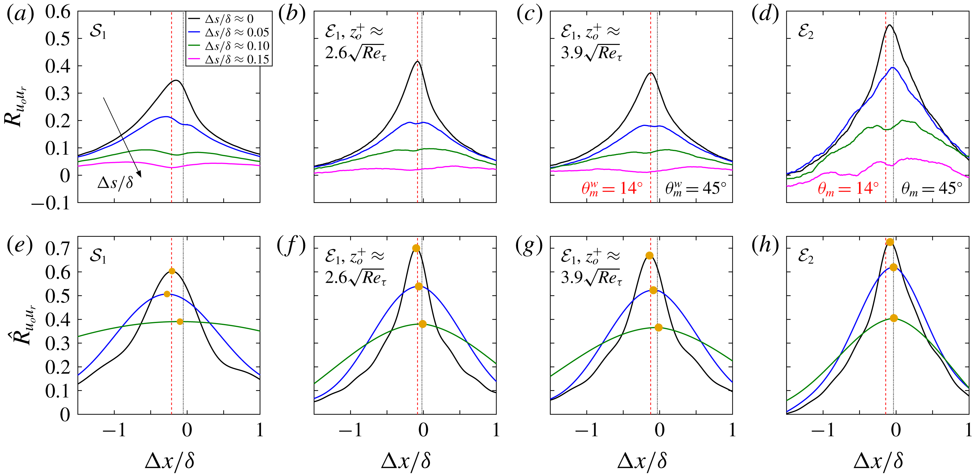
 $\unicode[STIX]{x0394}s/\unicode[STIX]{x1D6FF}$
, for data sets listed in table 2. (a–d) and (e–h) are correlations obtained from raw and large-wavelength-pass-filtered velocity time series, respectively, with a filter cutoff
 $\unicode[STIX]{x1D706}_{x,c}(z_{o},z_{r},\unicode[STIX]{x0394}s)$
based on
 $\unicode[STIX]{x1D6FE}_{L}^{2}(z_{o},z_{r},\unicode[STIX]{x0394}s)=0.05$
computed for respective data sets. Red dashed and grey dot-dashed lines indicate
 $\unicode[STIX]{x0394}x/\unicode[STIX]{x1D6FF}$
corresponding to
 $\unicode[STIX]{x1D703}_{m}^{w}=14^{\circ }$
and
 $45^{\circ }$
, respectively, for data sets
 ${\mathcal{E}}_{1}$
and
 ${\mathcal{S}}_{1}$
, and
 $\unicode[STIX]{x1D703}_{m}=14^{\circ }$
and
 $45^{\circ }$
, respectively, for data set
 ${\mathcal{E}}_{2}$
. Here,
 $\unicode[STIX]{x1D703}_{m}=\text{atan}((z_{o}-z_{r})/\unicode[STIX]{x0394}x_{p})$
. Yellow bullets in (e–h) highlight the peak in the cross-correlation.

4.2 Variation of mean structure inclination angle with spanwise offset
Having verified that large wall-attached structures are isolated on increasing
 $\unicode[STIX]{x0394}s$
between probes at
 $z_{r}$
and
 $z_{o}$
, we now investigate the variation of
 $\unicode[STIX]{x1D703}_{m}$
(with
 $\unicode[STIX]{x0394}s$
) by locating the peak (Marusic & Heuer Reference Marusic and Heuer2007) in the correlation coefficient (
 $R_{u_{o}u_{r}}$
) obtained on cross-correlating raw (unfiltered) velocity data from the two probes as follows:
 $$\begin{eqnarray}R_{u_{o}u_{r}}(\unicode[STIX]{x0394}x,\unicode[STIX]{x0394}s)=\frac{\langle u(z_{r};x,y)u(z_{o};x+\unicode[STIX]{x0394}x,y+\unicode[STIX]{x0394}s)\rangle }{\sqrt{\langle u^{2}(z_{r})\rangle }\sqrt{\langle u^{2}(z_{o})\rangle }};\end{eqnarray}$$
 $R_{u_{o}u_{r}}(\unicode[STIX]{x0394}x)$
for the three data sets, at selected
 $\unicode[STIX]{x0394}s$
, is plotted in figure 3(a–d). It may be observed that the correlation curve changes from having a clear distinct peak at
 $\unicode[STIX]{x0394}s\approx 0$
to one exhibiting a bi-modal behaviour as
 $\unicode[STIX]{x0394}s$
increases, for all data sets. The magnitude of the peak also drops significantly, making it difficult to locate a unique peak and associate it with the streamwise delay (
 $\unicode[STIX]{x0394}x_{p}$
) corresponding to the inclination of the mean structure. It is interesting to note that one of these two peaks in
 $R_{u_{o}u_{r}}$
is consistently close to
 $\unicode[STIX]{x0394}x\sim 0$
for all the data sets. Since
 $\unicode[STIX]{x0394}x\sim 0$
corresponds to
 $\unicode[STIX]{x1D703}_{m}^{w}\sim 90^{\circ }$
, this peak may be associated with the randomly oriented structures (for example, isotropic structures), which are known (Alving et al.
Reference Alving, Smits and Watmuff1990) to bias the cross-correlation towards
 $\unicode[STIX]{x1D703}_{m}^{w}\sim 90^{\circ }$
and negligibly contribute to the covariance (that is, the numerator in (4.2)). It is quite possible that some of these structures, which have no preferred inclination angle, may also be coherent across the two probes, apart from the majority forward-inclined structures (Perry et al.
Reference Perry, Uddin and Marusic1992). To make things clearer, the velocity data at both
 $z_{o}$
and
 $z_{r}$
are passed through a long-wavelength pass filter with a filter bound
 $\unicode[STIX]{x1D706}_{x,c}(z_{o},z_{r},\unicode[STIX]{x0394}s)$
obtained from the corresponding
 $\unicode[STIX]{x1D6FE}_{filt}^{2}(z_{o},z_{r},\unicode[STIX]{x0394}s)=0.05$
for the three data sets (refer § 4.1). Application of this filter ensures that only those streamwise wavelengths are considered which have been stochastically found to be coherent between the two probes for various
 $\unicode[STIX]{x0394}s$
(that is, wall-attached).
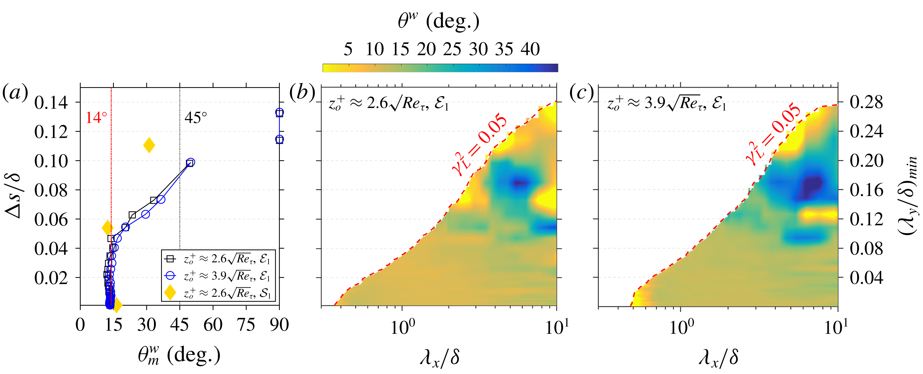
(a) Average structure inclination angle (
 $\unicode[STIX]{x1D703}_{m}^{w}$
) as a function of
 $\unicode[STIX]{x0394}s/\unicode[STIX]{x1D6FF}$
obtained by locating the peak of
 $\hat{R}_{u_{o}u_{r}}$
for data sets
 ${\mathcal{E}}_{1}$
and
 ${\mathcal{S}}_{1}$
. (b,c) Scale-specific phase (
 $\unicode[STIX]{x1D6F7}$
) of the cross-spectra (
 $\unicode[STIX]{x1D719}_{u_{o}u_{r}}^{\prime }$
), computed at various
 $\unicode[STIX]{x0394}s$
, expressed as a physical inclination angle (
 $\unicode[STIX]{x1D703}^{w}$
) for
 $z_{o}^{+}\approx$
(b)
 $2.6\sqrt{Re_{\unicode[STIX]{x1D70F}}}$
and (c)
 $3.9\sqrt{Re_{\unicode[STIX]{x1D70F}}}$
for data set
 ${\mathcal{E}}_{1}$
.

On filtering the velocity data, the new cross-correlation coefficient (
 $\hat{R}_{u_{o}u_{r}}$
) is computed by replacing
 $u(z_{o})$
and
 $u(z_{r})$
with their filtered counterparts,
 $\hat{u} (z_{o})$
and
 $\hat{u} (z_{r})$
in (4.2), and is plotted in figure 3(e–h). Since
 $\unicode[STIX]{x1D706}_{x,c}$
increases with
 $\unicode[STIX]{x0394}s$
,
 $\hat{R}_{u_{o}u_{r}}$
becomes wider about the peak with increasing
 $\unicode[STIX]{x0394}s$
. It is evident that the filtering aids in identification of a clear peak (highlighted by a yellow bullet) of the cross-correlation, with the associated correlation coefficient also having a significant value. The peak can be seen deviating from
 $\unicode[STIX]{x0394}x/\unicode[STIX]{x1D6FF}$
corresponding to
 $\unicode[STIX]{x1D703}_{m}=14^{\circ }$
(observed by Marusic & Heuer Reference Marusic and Heuer2007) towards that for
 $45^{\circ }$
with increasing
 $\unicode[STIX]{x0394}s$
. This observation supports our hypothesis proposed in § 2 that
 $\unicode[STIX]{x1D703}_{m}\rightarrow \unicode[STIX]{x1D703}_{s}$
on increasing the spanwise offset between the two probes.
Here,
 $\unicode[STIX]{x1D703}_{m}^{w}$
obtained from
 $\hat{R}_{u_{o}u_{r}}$
for data sets
 ${\mathcal{E}}_{1}$
and
 ${\mathcal{S}}_{1}$
, at various
 $\unicode[STIX]{x0394}s$
, is plotted in figure 4(a). Indeed,
 $\unicode[STIX]{x1D703}_{m}^{w}$
increases from approximately
 $14^{\circ }$
at
 $\unicode[STIX]{x0394}s\approx 0$
with increasing
 $\unicode[STIX]{x0394}s$
, reaching close to
 $50^{\circ }$
at
 $\unicode[STIX]{x0394}s/\unicode[STIX]{x1D6FF}\approx 0.1$
, after which it jumps abruptly to
 $90^{\circ }$
for larger offsets. This jump to
 $90^{\circ }$
suggests that eddies with an inherent forward inclination do not span across such large offsets, and the coherence,
 $\unicode[STIX]{x1D6FE}_{L}^{2}\lesssim 0.1$
, may be due to the randomly oriented eddies (Perry et al.
Reference Perry, Uddin and Marusic1992) co-existing in the TBL. These eddies tend to bias the cross-correlation peak towards
 $\unicode[STIX]{x0394}x\sim 0$
(Alving et al.
Reference Alving, Smits and Watmuff1990), which represents
 $\unicode[STIX]{x1D703}_{m}^{w}\sim 90^{\circ }$
and has been observed in
 $R_{u_{o}u_{r}}$
plotted in figure 3. Taking this into consideration, the largest physically realistic values of
 $\unicode[STIX]{x1D703}_{m}^{w}$
are found to be approximately
 $35^{\circ }$
and
 $50^{\circ }$
at
 $\unicode[STIX]{x0394}s/\unicode[STIX]{x1D6FF}\approx 0.08$
and 0.10, respectively, which are both close to the theoretically supported angle of
 $45^{\circ }$
(§ 1). This encourages us to conclude that
 $\unicode[STIX]{x1D703}_{s}^{w}$
is indeed nominally
 $45^{\circ }$
for a large isolated flow structure. A similar trend of increasing
 $\unicode[STIX]{x1D703}_{m}^{w}$
, with increasing
 $\unicode[STIX]{x0394}s$
, is also observed for the
 ${\mathcal{S}}_{1}$
data set (not shown completely for brevity), but the increment rate is relatively slow, probably due to the limited streamwise scale range owing to the domain size selected for the analysis (discussed in § 4.1). Since the coherence becomes lower than the threshold (
 $\unicode[STIX]{x1D6FE}_{L}^{2}\lesssim 0.05$
) across all
 $\unicode[STIX]{x1D706}_{x}$
for
 $\unicode[STIX]{x0394}s/\unicode[STIX]{x1D6FF}\gtrsim 0.15$
, no cross-correlation (and
 $\unicode[STIX]{x1D703}_{m}$
) is obtained for such spans after filtering.
4.3 Scale-specific inclination angle of wall-attached structures
Analysing the cross-correlation yields
 $\unicode[STIX]{x1D703}_{m}$
, which is influenced by a range of scales (Marusic Reference Marusic2001). Since we see an increase in
 $\unicode[STIX]{x1D703}_{m}^{w}$
towards
 $45^{\circ }$
with an increase in
 $\unicode[STIX]{x0394}s$
(figure 4
a), it would be interesting to see how a streamwise-scale-specific inclination angle (
 $\unicode[STIX]{x1D703}^{w}(\unicode[STIX]{x1D706}_{x})$
) varies with
 $\unicode[STIX]{x0394}s$
. Following Baars et al. (Reference Baars, Hutchins and Marusic2016),
 $\unicode[STIX]{x1D703}^{w}$
is obtained from the scale-dependent phase information embedded in the cross-spectrum (
 $\unicode[STIX]{x1D719}_{u_{o}u_{r}}^{\prime }$
);
 $\unicode[STIX]{x1D719}_{u_{o}u_{r}}^{\prime }(\unicode[STIX]{x0394}s;\unicode[STIX]{x1D706}_{x})={\mathcal{F}}[R_{u_{o}u_{r}}(\unicode[STIX]{x0394}s;\unicode[STIX]{x0394}x)]$
has already been computed to find
 $\unicode[STIX]{x1D6FE}_{L}^{2}$
in (4.1) and is complex-valued. The scale-specific phase (
 $\unicode[STIX]{x1D6F7}$
) is estimated from
 $\unicode[STIX]{x1D719}_{u_{o}u_{r}}^{\prime }$
as follows:
 $$\begin{eqnarray}\unicode[STIX]{x1D6F7}(\unicode[STIX]{x0394}s;\unicode[STIX]{x1D706}_{x})=\text{atan}\left\{\frac{\text{Im}[\unicode[STIX]{x1D719}_{u_{o}u_{r}}^{\prime }(\unicode[STIX]{x0394}s;\unicode[STIX]{x1D706}_{x})]}{\text{Re}[\unicode[STIX]{x1D719}_{u_{o}u_{r}}^{\prime }(\unicode[STIX]{x0394}s;\unicode[STIX]{x1D706}_{x})]}\right\},\end{eqnarray}$$
where Im and Re denote the imaginary and real components of
 $\unicode[STIX]{x1D719}_{u_{o}u_{r}}^{\prime }$
. We find
 $\unicode[STIX]{x1D6F7}$
essentially records the shift of each Fourier mode,
 $\unicode[STIX]{x1D706}_{x}$
, owing to the correlation of
 $u$
measured at two different wall-normal locations. A streamwise shift (
 $\ell (\unicode[STIX]{x0394}s;\unicode[STIX]{x1D706}_{x})$
) is obtained from the phase (which is in radians) by pre-multiplying it with the respective Fourier mode – that is,
 $\ell (\unicode[STIX]{x0394}s;\unicode[STIX]{x1D706}_{x})=\unicode[STIX]{x1D706}_{x}\unicode[STIX]{x1D6F7}(\unicode[STIX]{x0394}s;\unicode[STIX]{x1D706}_{x})/(2\unicode[STIX]{x03C0})$
. A scale-specific physical inclination angle is then computed at each
 $\unicode[STIX]{x0394}s$
following
 $$\begin{eqnarray}\unicode[STIX]{x1D703}^{w}(\unicode[STIX]{x0394}s;\unicode[STIX]{x1D706}_{x})=\text{atan}\left\{\frac{(z_{o}-z_{r})}{\ell (\unicode[STIX]{x0394}s;\unicode[STIX]{x1D706}_{x})}\right\};\end{eqnarray}$$
 $\unicode[STIX]{x1D703}^{w}(\unicode[STIX]{x1D706}_{x},\unicode[STIX]{x0394}s)$
is plotted in figure 4(b) and (c) for
 $z_{o}^{+}\approx 2.6\sqrt{Re_{\unicode[STIX]{x1D70F}}}$
and
 $3.9\sqrt{Re_{\unicode[STIX]{x1D70F}}}$
, respectively, for data set
 ${\mathcal{E}}_{1}$
. Here, we restrict our attention to streamwise wavelengths
 $\unicode[STIX]{x1D706}_{x}/\unicode[STIX]{x1D6FF}\leqslant 10$
so that the interpretation of
 $\unicode[STIX]{x1D703}^{w}$
is not influenced by the assumption of Taylor’s hypothesis (de Silva et al.
Reference de Silva, Squire, Hutchins and Marusic2015).
It can be seen in both figure 4(b,c) that
 $\unicode[STIX]{x1D703}^{w}$
, in general, increases with
 $\unicode[STIX]{x0394}s$
and corresponds well with the variation of
 $\unicode[STIX]{x1D703}_{m}^{w}$
shown in figure 4(a). At
 $\unicode[STIX]{x0394}s\approx 0$
, all the wall-coherent scales agree to an almost constant angle of
 $\unicode[STIX]{x1D703}^{w}\approx 14^{\circ }$
, even at large
 $\unicode[STIX]{x1D706}_{x}$
(Baars et al.
Reference Baars, Hutchins and Marusic2016). This is because
 $\unicode[STIX]{x1D703}^{w}$
, here, is influenced by structures with
 $0<\unicode[STIX]{x1D706}_{y}<\infty$
, meaning that not all the influencing structures are large in the two-dimensional sense. As
 $\unicode[STIX]{x0394}s/\unicode[STIX]{x1D6FF}>0.04$
,
 $\unicode[STIX]{x1D703}^{w}$
increases across all
 $\unicode[STIX]{x1D706}_{x}>\unicode[STIX]{x1D706}_{x,c}$
since only structures of spanwise wavelength
 $\unicode[STIX]{x1D706}_{y}/\unicode[STIX]{x1D6FF}>0.08$
influence the estimation. It is around this
 $\unicode[STIX]{x0394}s/\unicode[STIX]{x1D6FF}$
range where
 $\unicode[STIX]{x1D703}_{m}^{w}$
starts deviating from
 $14^{\circ }$
(figure 4
a). On increasing
 $\unicode[STIX]{x0394}s/\unicode[STIX]{x1D6FF}$
to 0.08, we are effectively considering only the large structures (
 $\unicode[STIX]{x1D706}_{x}/\unicode[STIX]{x1D6FF}>2$
,
 $\unicode[STIX]{x1D706}_{y}/\unicode[STIX]{x1D6FF}>0.16$
) for which
 $\unicode[STIX]{x1D703}^{w}\gtrsim 30^{\circ }$
, which aligns well with the previous estimations (
 $\unicode[STIX]{x1D703}_{s}$
; table 1) made via visualizing individual structures. It also explains the average estimation
 $\unicode[STIX]{x1D703}_{m}^{w}\approx 45^{\circ }$
at similar offsets. The qualitatively similar variation of
 $\unicode[STIX]{x1D703}^{w}(\unicode[STIX]{x0394}s;\unicode[STIX]{x1D706}_{x})$
for both
 $z_{o}^{+}$
, especially at high
 $\unicode[STIX]{x0394}s$
(figure 4
b,c), reinforces the fact that our conclusions should be applicable for all
 $z_{o}^{+}$
in the log region. It is difficult to physically interpret
 $\unicode[STIX]{x1D703}^{w}$
for
 $\unicode[STIX]{x0394}s/\unicode[STIX]{x1D6FF}>0.11$
given that
 $\unicode[STIX]{x1D703}_{m}^{w}$
abruptly jumps to
 $90^{\circ }$
for these offsets (figure 4
a), suggesting a contribution from randomly oriented structures to the cross-correlation.
4.4 Implications on LES and AEH-based simulations
Having empirically established that
 $\unicode[STIX]{x1D703}_{s}^{w}\approx 45^{\circ }$
(nominally) for isolated large wall-attached eddies, we now discuss possible implications of the findings of the present study on LES and AEH-based simulations. In recent AEH-based simulations (Baidya et al.
Reference Baidya, Philip, Monty, Hutchins and Marusic2014, Reference Baidya, Philip, Hutchins, Monty and Marusic2017; Chandran et al.
Reference Chandran, Baidya, Monty and Marusic2017),
 $\unicode[STIX]{x1D6EC}$
-vortices organized in a packet are typically used as representative structures to statistically model the log region of a ZPG TBL. Simulation results reported by Marusic (Reference Marusic2001) clearly indicate that the size and shape, as well as the orientation of the eddies, significantly influence the statistics yielded by the model. Over the years, researchers have attempted to improvise on the size and shape of the representative eddies (Marusic & Monty Reference Marusic and Monty2019), via trial and error, to mimic the experimental trends. However, in the case of the orientation of the individual eddies (
 $\unicode[STIX]{x1D703}_{s}^{w}$
), considering support from the theory (§ 1) as well as flow visualizations reported in the seminal studies of Head & Bandyopadhyay (Reference Head and Bandyopadhyay1981) and others,
 $\unicode[STIX]{x1D703}_{s}^{w}$
has always been assumed to be nominally
 $45^{\circ }$
. This trend has continued over the years without any concrete empirical evidence, which this study has attempted to address. Here, via physical and statistical filters, we have isolated the large wall-attached eddies and have empirically shown that
 $\unicode[STIX]{x1D703}_{s}^{w}$
is nominally
 $45^{\circ }$
for these eddies, suggesting it to be a reasonable assumption for the orientation of the individual
 $\unicode[STIX]{x1D6EC}$
-vortices considered for an AEH-based simulation.
Moving to the implication on LES simulations, due to limitations in computational power, high-
 $Re_{\unicode[STIX]{x1D70F}}$
LES simulations typically only compute the outer layer of the TBL (Piomelli & Balaras Reference Piomelli and Balaras2002). The grid resolution for the simulation is thus chosen based on the outer layer eddies, making it incapable of resolving the relatively small eddies existing in the inner layer of the TBL, and in turn also limiting estimation of the wall shear stress (
 $\unicode[STIX]{x1D70F}_{w}$
). In such a scenario, information from the computed outer flow is utilized to estimate
 $\unicode[STIX]{x1D70F}_{w}$
(Marusic, Kunkel & Porte-Agel Reference Marusic, Kunkel and Porte-Agel2001), wherein the inclination of the elongated eddies in the inner layer needs to be accounted for. Earlier studies (Piomelli et al.
Reference Piomelli, Ferziger, Moin and Kim1989; Carper & Porte-Agel Reference Carper and Porte-Agel2004) have used the experimentally obtained value of
 $\unicode[STIX]{x1D703}_{m}^{w}\approx 14^{\circ }$
as the mean inclination of these eddies. However, the empirical observations in the present study (figure 4
a) in conjunction with the simulations of Marusic (Reference Marusic2001) strongly suggest that
 $\unicode[STIX]{x1D703}_{m}^{w}$
depends on the range of scales being considered in the flow. Since the inclination angle of solely the unresolved structures in the inner layer needs to be taken into account while estimating
 $\unicode[STIX]{x1D70F}_{w}$
,
 $\unicode[STIX]{x1D703}_{m}^{w}$
for these selective range of scales may be a function of the grid resolution and consequently may differ from
 $14^{\circ }$
.
5 Concluding remarks
The streamwise inclination angle of large wall-attached structures, in the log region of a TBL, is estimated statistically to be nominally
 $45^{\circ }$
. This result was estimated by isolating these structures from the remaining assemblage of eddies by introducing a spanwise offset between the near-wall and log-region reference probe – a methodology which was shown to be effective for TBL data sets across
 $Re_{\unicode[STIX]{x1D70F}}\sim O(10^{3})$
–
 $O(10^{6})$
. The angle obtained closely resembles the inclination of individual ‘hairpin’-type structures considered to be the dominant feature of a wall-bounded turbulent flow (Moin & Kim Reference Moin and Kim1985), suggesting wall-attached structures to be of similar type. The present findings also provide empirical evidence in support of the eddy inclination angles considered when simulating a TBL with AEH-based simulations. Although the empirical result,
 $\unicode[STIX]{x1D703}_{s}^{w}\approx 45^{\circ }$
, may be limited to large wall-attached structures, theoretical arguments discussed in § 1 give a strong indication of what the approximate
 $\unicode[STIX]{x1D703}_{s}^{w}$
of relatively smaller wall-attached structures would be. The present findings may also have implications for the wall-layer models employed in high-
 $Re_{\unicode[STIX]{x1D70F}}$
LES simulations of a TBL, which utilize experimentally determined
 $\unicode[STIX]{x1D703}_{m}^{w}$
to correlate wall shear stress with the velocity estimated at the near-wall grid point. The present analysis reveals that
 $\unicode[STIX]{x1D703}_{m}^{w}$
is a function of the range of scales considered for its estimation, and this range would vary with the grid size considered for the LES simulation.
Acknowledgements
The authors wish to acknowledge the Australian Research Council for financial support and appreciate the publicly available DNS data of Sillero et al. (Reference Sillero, Jiménez and Moser2013).