


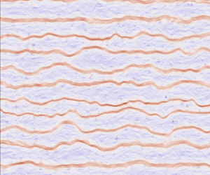





1. Introduction
Perturbations to a barotropic (i.e. depth-independent) fluid with a background potential vorticity gradient,  $\beta >0$, propagate westward as Rossby waves. In a turbulent flow, the nonlinear interplay between Rossby waves and turbulence results in the latitudinally inhomogeneous mixing of potential vorticity, which, through a positive dynamical feedback, spontaneously reorganizes the flow into one characterized by eastward jets (Dritschel & McIntyre Reference Dritschel and McIntyre2008). The ultimate limit of such inhomogeneous mixing, which can be achieved for sufficiently large values of
 $\beta$, is a potential vorticity staircase: a piecewise constant potential vorticity profile consisting of well-mixed regions separated by isolated discontinuities, with eastward jets centred at the discontinuities and westward flows in between (Danilov & Gurarie Reference Danilov and Gurarie2004; Dunkerton & Scott Reference Dunkerton and Scott2008; Scott & Dritschel Reference Scott and Dritschel2012, Reference Scott and Dritschel2019).
Analogously, a buoyancy gradient at the surface of a quasigeostrophic fluid supports the existence of surface-trapped Rossby waves that are less dispersive than their barotropic counterparts (Held et al. Reference Held, Pierrehumbert, Garner and Swanson1995; Lapeyre Reference Lapeyre2017). The purpose of this article is to investigate the formation of zonal jets in the presence of a background surface buoyancy gradient and to examine the realizability of surface buoyancy staircases in the surface quasigeostrophic model. Although the present study is the first to systematically investigate the emergence of surface quasigeostrophic jets, there are previous studies which make use of the uniformly stratified surface quasigeostrophic model with a background buoyancy gradient. These include Smith et al. (Reference Smith, Boccaletti, Henning, Marinov, Tam, Held and Vallis2002), who derive the dependence of the diffusion coefficient of a passive tracer in the presence a background buoyancy gradient. Another is Sukhatme & Smith (Reference Sukhatme and Smith2009), who, in their investigation of  $\alpha$-turbulence models with a background gradient, note that, because of the decreased interaction range, surface quasigeostrophic jets in uniform stratification should be narrower than their counterparts in the barotropic model. Finally, Lapeyre (Reference Lapeyre2017) demonstrates that jets can indeed form in the uniformly stratified surface quasigeostrophic model.
We also investigate how surface quasigeostrophic jets depend on the underlying vertical stratification. Yassin & Griffies (Reference Yassin and Griffies2022) show that the vertical stratification modifies the interaction range of vortices in the surface quasigeostrophic model. Suppose we have an infinitely deep fluid governed by the time-evolution of geostrophic buoyancy anomalies at its upper boundary. Then if the stratification is decreasing ( $N'(z)\leq 0$, where
 $N(z)$ is buoyancy frequency) towards the fluid's surface (that is, the upper boundary), then the interaction range is longer than in the uniformly stratified model and the resulting turbulence is characterized by thin buoyancy filaments – analogous to the thin vorticity filaments in two-dimensional barotropic turbulence. Conversely, if the stratification is increasing (
 $N'(z)\geq 0$) towards the surface, then the interaction range is shorter than in uniform stratification, and the buoyancy field appears spatially diffuse and lacks thin filamentary structures. In this article, we find that the interaction range is related to Rossby wave dispersion: flows with a longer interaction range have more dispersive Rossby waves whereas flows with a shorter interaction range have less dispersive Rossby waves. One of our aims is to characterize the dependence of surface quasigeostrophic jets on the functional form of the vertical stratification.
There are two motivations behind the present work. The first is its potential relevance to the upper ocean. Buoyancy anomalies at the ocean's surface are governed by the surface quasigeostrophic model (Isern-Fontanet et al. Reference Isern-Fontanet, Chapron, Lapeyre and Klein2006; LaCasce & Mahadevan Reference LaCasce and Mahadevan2006; Lapeyre & Klein Reference Lapeyre and Klein2006). Both numerical (Isern-Fontanet et al. Reference Isern-Fontanet, Lapeyre, Klein, Chapron and Hecht2008; Lapeyre Reference Lapeyre2009; Qiu et al. Reference Qiu, Chen, Klein, Ubelmann, Fu and Sasaki2016, Reference Qiu, Chen, Klein, Torres, Wang, Fu and Menemenlis2020; Miracca-Lage et al. Reference Miracca-Lage, González-Haro, Napolitano, Isern-Fontanet and Polito2022) as well as observational (González-Haro & Isern-Fontanet Reference González-Haro and Isern-Fontanet2014) studies indicate that a significant fraction of the surface geostrophic velocity is induced by sea surface buoyancy anomalies. Surface buoyancy anomalies largely induce the surface geostrophic velocities over major subtropical currents (e.g. the Gulf Stream and Kurushio) in wintertime, and over the Southern Ocean all year round. Moreover, upper ocean turbulence has been found to be anisotropic (Maximenko, Bang & Sasaki Reference Maximenko, Bang and Sasaki2005; Scott et al. Reference Scott, Arbic, Holland, Sen and Qiu2008), with significant differences in anisotropy between major extratropical currents and other regions in the ocean (Wang et al. Reference Wang, Qiao, Dai and Zhou2019). The appropriate model to study anisotropy under these conditions is the surface quasigeostrophic model.
The second motivation is that the variable stratification surface quasigeostrophic model is a simple two-dimensional model in which we can investigate how jet dynamics depend on the stratification's vertical structure. Another such model is the equivalent barotropic model for which the deformation radius represents the rigidity of the free surface. At sufficiently large scales, small values of the deformation radius lead to a pliable free surface allowing a significant degree of horizontal divergence. The resulting flow then has an exponentially short interaction range, with a horizontal attenuation of the order of the deformation radius (Polvani, Zabusky & Flierl Reference Polvani, Zabusky and Flierl1989), and with approximately non-dispersive Rossby waves. Consequently, for a finite deformation radius, we obtain jets whose width is of the order of the deformation radius with a fixed meandering shape (Scott, Burgess & Dritschel Reference Scott, Burgess and Dritschel2022). In contrast, for the variable stratification surface quasigeostrophic model, rather than just specifying a constant (i.e. the deformation wavenumber), one instead has to specify the stratification's functional form,  $N(z)$. Over decreasing stratification
 $(N'(z) <0)$, because of the longer interaction range and the more dispersive waves, we obtain jets similar to the two-dimensional barotropic model. Conversely, over increasing stratification
 $(N'(z)>0)$, the shorter interaction range along with the weakly dispersive waves lead to sinuous jets whose shape evolves in time through the propagation of weakly dispersive along jet waves. Moreover, because of these along jet waves, a smaller fraction of the total energy is contained in the zonal mode over increasing stratification (with a shorter interaction range) than over decreasing stratification (with a longer interaction range).
The remainder of this article is organized as follows. Section 2 introduces the variable stratification surface quasigeostrophic model and shows how the stratification's vertical structure controls both the interaction range of point vortices as well as the dispersion of surface-trapped Rossby waves. Then, in § 3, we introduce two wavenumbers,  $k_\varepsilon$ and
 $k_r$, whose ratio,
 $k_\varepsilon /k_r$, forms the key non-dimensional parameter of this study; here,
 $k_\varepsilon$ is a wavenumber depending on the energy injection rate whereas
 $k_r$ is a wavenumber depending on surface damping rate. This non-dimensional number is a generalization of the non-dimensional number used in previous studies (Danilov & Gurarie Reference Danilov and Gurarie2002; Sukoriansky, Dikovskaya & Galperin Reference Sukoriansky, Dikovskaya and Galperin2007; Scott & Dritschel Reference Scott and Dritschel2012). By considering an idealized buoyancy staircase, we also investigate how the Rhines wavenumber relates to the jet spacing under decreasing, increasing and uniform stratification. Section 4 then presents numerical experiments detailing the emergence of the staircase limit as
 $k_\varepsilon /k_r$ is increased for various stratification profiles. In addition, we also present experiments where we fix the external parameters and vary the vertical stratification alone. Finally, we conclude in § 5.
2. The interaction range and wave dispersion
2.1. Equations of motion
Consider an infinitely deep Boussinesq fluid with zero interior potential vorticity. The geostrophic stream function,  $\psi$, then satisfies
 \begin{equation} \frac{\partial{}}{\partial{z}}\left(\frac{1}{\sigma^2} \frac{\partial{\psi}}{\partial{z}} \right) + \nabla^2 \psi = 0 \end{equation}
in the fluid interior,  $z \in (-\infty,0)$. The horizontal Laplacian is denoted by
 $\nabla ^2 = \partial _x^2 + \partial _y^2$ and the non-dimensional stratification is given by
 \begin{equation} \sigma(z) = N(z)/f, \end{equation}
where  $N(z)$ is the buoyancy frequency and
 $f$ is the constant local value of the Coriolis parameter. Time-evolution is determined by the material conservation of surface potential vorticity (Bretherton Reference Bretherton1966),
 \begin{equation} \theta = \left.-\frac{1}{\sigma_0^2} \frac{\partial{\psi}}{\partial{z}}\right|_{z=0}, \end{equation}
at the upper boundary,  $z=0$, where
 $\sigma _0 = \sigma (0)$. Explicitly, the time-evolution equation is
 \begin{equation} \frac{\partial{\theta}}{\partial{t}} + J(\psi,\theta) + \varLambda \partial_x \psi = F-D, \end{equation}
at  $z=0$, where
 $J(\psi,\theta ) = \partial _x \psi \partial _y \theta - \partial _x \theta \partial _y \psi$ represents the advection of
 $\theta$ by the geostrophic velocity,
 $\boldsymbol {u} = \hat {\boldsymbol {z}} \times \boldsymbol {\nabla } \psi$. The frequency,
 $\varLambda$, is given by
 \begin{equation} \varLambda ={-} \frac{1}{f\sigma_0^2} \frac{\mathrm{d} B}{\mathrm{d} y}, \end{equation}
where  $B(y,z)$ is the background buoyancy field. By geostrophic balance, this buoyancy field induces a zonal geostrophic flow,
 $U(z)$, related to
 $B(y,z)$ through
 \begin{equation} \left.\frac{\mathrm{d} B}{\mathrm{d} y}\right|_{z=0} ={-} f \, \frac{\mathrm{d} U}{\mathrm{d} z}. \end{equation}
Without loss of generality, we have assumed that  $U(0)=0$ in the time-evolution equation (2.4) to eliminate a constant advective term. The dissipation,
 $D$, consists of linear damping and small-scale dissipation,
 \begin{equation} D = r \, \theta + {\textit{ssd}}, \end{equation}
where  $r$ is the surface buoyancy damping rate. We use linear damping because it allows us to compute the equilibrium energy using only the energy injection rate (see § 3). The forcing,
 $F$, and the small-scale dissipation,
 ${\textit{ssd}}$, are described in § 4.
The background zonal geostrophic flow,  $U(z)$, must satisfy the zero potential vorticity condition (2.1), given by
 \begin{equation} \frac{\mathrm{d} }{\mathrm{d} z} \left(\frac{1}{\sigma^2}\frac{\mathrm{d} U}{\mathrm{d} z} \right) = 0. \end{equation}
This condition, although seemingly artificial, is appropriate for our study, which focuses on jet formation at a fluid boundary where the geostrophic velocity is determined by buoyancy anomalies at that boundary. As discussed in the introduction, this situation is common in the ocean (González-Haro & Isern-Fontanet Reference González-Haro and Isern-Fontanet2014; Yassin & Griffies Reference Yassin and Griffies2022). As long as the geostrophic velocity at the boundary is primarily determined by buoyancy anomalies at that boundary, the presence or absence of interior potential vorticity should only impact the dynamics in the interior, which is not the focus of our study.
The surface buoyancy anomaly,  $b|_{z=0}$, is related to the surface potential vorticity,
 $\theta$, through
 \begin{equation} b|_{z=0} ={-} f\,\sigma_0^2 \theta. \end{equation}
Therefore, the time-evolution equation (2.4) equivalently states that surface buoyancy anomalies are materially conserved in the absence of forcing and dissipation.
If we further assume a doubly periodic domain in the horizontal, then we can expand the stream function as
 \begin{equation} \psi(\boldsymbol{r}, z,t) = \sum_{\boldsymbol{k}} \hat \psi_{\boldsymbol{k}}(t) \, \varPsi_k(z)\, \mathrm{e}^{\mathrm{i} \boldsymbol{k}\, \boldsymbol{\cdot}\, \boldsymbol{x}}, \end{equation}
where  $\boldsymbol {x}=(x,y)$ is the horizontal position vector,
 $z$ is the vertical coordinate,
 $\boldsymbol {k} = (k_x,k_y)$ is the horizontal wavevector,
 $k=\left \lvert \boldsymbol {k} \right \rvert$ is the horizontal wavenumber and
 $t$ is the time coordinate. The non-dimensional wavenumber-dependent vertical structure,
 $\varPsi _k(z)$, is determined by the boundary value problem (Yassin & Griffies Reference Yassin and Griffies2022)
 \begin{equation} -\frac{\mathrm{d} }{\mathrm{d} z} \left(\frac{1}{\sigma^2}\frac{\mathrm{d} \varPsi_k}{\mathrm{d} z}\right) + k^2 \varPsi_k(z) = 0, \end{equation}
with the upper boundary condition
 \begin{equation} \varPsi_k(0)=1, \end{equation}
and lower boundary condition
 \begin{equation} \varPsi_k \rightarrow 0, \quad \text{as } \ z \rightarrow -\infty. \end{equation}
The upper boundary condition (2.12) is a normalization for the vertical structure,  $\varPsi _k(z)$, chosen so that
 \begin{equation} \psi(\boldsymbol{r}, z=0,t) = \sum_{\boldsymbol{k}} \hat \psi_{\boldsymbol{k}}(t) \, \mathrm{e}^{\mathrm{i} \boldsymbol{k}\, \boldsymbol{\cdot}\, \boldsymbol{x}}. \end{equation}
The corresponding Fourier expansion of the surface potential vorticity is given by
 \begin{equation} \theta(\boldsymbol{r}, t) = \sum_{\boldsymbol{k}} \hat \theta_{\boldsymbol{k}}(t) \, \mathrm{e}^{\mathrm{i} \boldsymbol{k}\, \boldsymbol{\cdot}\, \boldsymbol{x}}, \end{equation}
where
 \begin{equation} \hat \theta_{\boldsymbol{k}} ={-} m(k) \, \hat \psi_{\boldsymbol{k}}, \end{equation}
and the function  $m(k)$ is given by
 \begin{equation} m(k) = \frac{1}{\sigma_0^2} \frac{\mathrm{d} \varPsi_k(0)}{\mathrm{d} z}. \end{equation}
The function  $m(k)$ relates
 $\hat \theta _{\boldsymbol {k}}$ to
 $\hat \psi _{\boldsymbol {k}}$ in the Fourier space inversion relation (2.16) and so we call
 $m(k)$ the inversion function.
To recover the well-known case of the uniformly stratified surface quasigeostrophic model (Held et al. Reference Held, Pierrehumbert, Garner and Swanson1995), set  $\sigma (z) = \sigma _0$. Then the vertical structure equation (2.11) along with boundary conditions (2.12) and (2.13) yield the exponentially decaying vertical structure
 $\varPsi _k(z) = \exp ({\sigma _0\,k\,z})$. On substituting
 $\varPsi _k(z)$ into (2.17), we obtain a linear inversion function
 \begin{equation} m(k) = \frac{k}{\sigma_0} \end{equation}
and hence (from the inversion relation (2.16)) a linear-in-wavenumber inversion relation  $\hat \theta _{\boldsymbol {k}} = - (k/\sigma _0) \, \hat \psi _{\boldsymbol {k}}$. We also recover a linear inversion function (2.18) in the small-scale limit; Yassin & Griffies (Reference Yassin and Griffies2022) show that
 $m(k)\rightarrow k/\sigma _0$ as
 $k\rightarrow \infty$ regardless of the functional form of
 $\sigma (z)$.
2.2. The inversion function and spatial locality
The inversion function  $m(k)$, which is determined by the stratification's vertical structure, controls the spatial locality of the resulting turbulence. We illustrate this point with the following piecewise stratification profile:
 \begin{equation} \sigma(z) = \begin{cases} \sigma_0, & \text{for} \ -h_{mix} < z < 0,\\ \sigma_0 + \Delta \sigma \left(\dfrac{z+h_{mix}}{h_{lin}}\right), & \text{for} \ -(h_{mix} + h_{lin}) < z <{-}h_{mix},\\ \sigma_{pyc}, & \text{for} \ -\infty < z <{-}(h_{mix} + h_{lin}) , \end{cases} \end{equation}
where  $\Delta \sigma =\sigma _0 - \sigma _{pyc}$. At small horizontal scales, where
 $k\gg k_s$, and
 \begin{equation} k_s=1/\left(\sigma_0\,h_{mix}\right), \end{equation}
then  $m(k) \approx k/\sigma _0$, as in the uniformly stratified model of Held et al. (Reference Held, Pierrehumbert, Garner and Swanson1995). Likewise, in the large-scale limit, where
 $k \ll k_{pyc}$, and
 \begin{equation} k_{pyc} = \begin{cases} 1/\left(\sigma_{pyc} h_{mix}\right), & \text{for} \ \Delta \sigma \leq 0, \\ \sigma_{pyc}/\left(\sigma_0^2 h_{mix}\right), & \text{for} \ \Delta \sigma>0, \end{cases} \end{equation}
then  $m(k) \approx k/\sigma _{pyc}$. However, for wavenumbers between
 $k_{pyc} \lesssim k \lesssim k_s$, the inversion function takes an approximate power law form
 \begin{equation} m(k) \approx m_0 k^{\alpha}, \end{equation}
where  $m_0>0$ and
 $\alpha \geq 0$. The power
 $\alpha$ depends on the ratio
 $\sigma _{pyc}/\sigma _0$ between the deep and surface stratification. If the stratification decreases towards the surface (
 $\sigma ^\prime (z) \leq 0$, or
 $\sigma _{pyc}/\sigma _0>1$) then
 $\alpha > 1$, with
 $\sigma _{pyc}/\sigma _0 \rightarrow \infty$ sending
 $\alpha \rightarrow 2$. In contrast, if the stratification increases towards the surface (
 $\sigma ^\prime (z) \geq 0$, or
 $\sigma _{pyc}/\sigma _0 < 1$) then
 $\alpha <1$, with
 $\sigma _{pyc}/\sigma _0 \rightarrow 0$ sending
 $\alpha \rightarrow 0$. Thus, for wavenumbers
 $k_{pyc} \lesssim k \lesssim k_s$, the inversion relation (2.16) has the approximate form
 \begin{equation} \hat \xi_{\boldsymbol{k}} ={-} k^\alpha \, \hat \psi_{\boldsymbol{k}}, \end{equation}
where  $\hat \xi _{\boldsymbol {k}}= \hat \theta _{\boldsymbol {k}}/m_0$, which is the inversion relation for
 $\alpha$-turbulence (Pierrehumbert, Held & Swanson Reference Pierrehumbert, Held and Swanson1994; Smith et al. Reference Smith, Boccaletti, Henning, Marinov, Tam, Held and Vallis2002; Sukhatme & Smith Reference Sukhatme and Smith2009). Figure 1 provides two examples, one with decreasing stratification (with
 $\alpha \approx 1.50$) and another with increasing stratification (with
 $\alpha \approx 0.49$).
The inversion functions, (a)  $m(k)$ for (b) two stratification profiles given by the piecewise stratification profile (2.19). One stratification profile is increasing (
 $\sigma '(z)\geq 0$, blue), with
 $\sigma _0=1$,
 $\sigma _{pyc}=0.15$,
 $h_{mix} = 0.01$ and
 $h_{lin}=0.05$. The other stratification profile is decreasing (
 $\sigma '(z)\leq 0$, red) with
 $\sigma _0=1$,
 $\sigma _{pyc}=10$,
 $h_{mix} = 0.01$ and
 $h_{lin}=0.05$. The thin black line is given by
 $k/\sigma _0$ where
 $\sigma _0=1$, whereas the blue and red lines are given by
 $k/\sigma _{pyc}$ with
 $\sigma _{pyc}=0.15$ for the thin blue line and
 $\sigma _{pyc}=10$ for the thin red line. Note that
 $m(k) \rightarrow k/\sigma _0$ as
 $k\rightarrow \infty$.

In addition to variable stratification, including a bottom boundary can also result in  $\alpha \neq 1$ at small wavenumbers. A free-slip bottom boundary condition leads to
 $m(k) \sim k^2$ at small
 $k$, which resembles two-dimensional barotropic turbulence at large spatial scales (Tulloch & Smith Reference Tulloch and Smith2006). In contrast, a no-slip bottom boundary condition leads to
 $m(k) \sim \mathrm {constant}$ at small
 $k$, which resembles the equivalent barotropic turbulence at large spatial scales (Yassin & Griffies Reference Yassin and Griffies2022). However, we do not explore the case with a bottom boundary any further.
To see how the parameter  $\alpha$ modifies the resulting dynamics, consider a point vortex at the origin, given by
 $\xi = \delta (\left \lvert \boldsymbol {x} \right \rvert )$, where
 $\left \lvert \boldsymbol {x} \right \rvert$ is the horizontal distance from the vortex centre, and
 $\delta (\left \lvert \boldsymbol {x} \right \rvert )$ is the Dirac delta. If
 $\alpha =2$, then the stream function induced by the point vortex is logarithmic,
 $\psi (\left \lvert \boldsymbol {x} \right \rvert ) = \log (\left \lvert \boldsymbol {x} \right \rvert )/(2{\rm \pi} )$. If
 $0 < \alpha < 2$, then
 $\psi (\left \lvert \boldsymbol {x} \right \rvert ) = -C_\alpha /\left \lvert \boldsymbol {x} \right \rvert ^{2-\alpha }$ where
 $C_\alpha >0$ is a constant (Iwayama & Watanabe Reference Iwayama and Watanabe2010). Smaller
 $\alpha$ leads to vortices with velocities decaying more quickly with the horizontal distance
 $\left \lvert \boldsymbol {x} \right \rvert$, and hence a shorter interaction range. Thus, the vertical stratification modifies the relationship between a surface buoyancy anomaly and its induced velocity field: a surface buoyancy anomaly over decreasing stratification (
 $\sigma '(z)\leq 0$) generates a longer range velocity field than an identical buoyancy anomaly over increasing stratification (
 $\sigma '(z)\geq 0$).
The parameter  $\alpha$ is also a measure of turbulence's spatial locality. For values of
 $\alpha$ close to
 $2$, the local fluid velocity is dominated by the large-scale strain induced by distant vortices and the flow is characterized by thin folding buoyancy filaments (Watanabe & Iwayama Reference Watanabe and Iwayama2004). As
 $\alpha$ is reduced to unity, buoyancy filaments become susceptible to an instability where they roll-up into small-scale vortices; consequently, the turbulence is characterized by vortices whose sizes span a wide range of horizontal scales (Pierrehumbert et al. Reference Pierrehumbert, Held and Swanson1994; Held et al. Reference Held, Pierrehumbert, Garner and Swanson1995). Finally, for small
 $\alpha$, the
 $\theta$ field becomes spatially diffuse as a result of the geostrophic velocity field having small spatial scales because such a velocity field is effective at mixing away small-scale inhomogeneities (Sukhatme & Smith Reference Sukhatme and Smith2009).
Both the  $\sigma _0>\sigma _{pyc}$ and the
 $\sigma _0 < \sigma _{pyc}$ are relevant to the ocean (Yassin & Griffies Reference Yassin and Griffies2022). At small-spatial scales, surface quasigeostrophic velocities are largely confined to the mixed-layer. Consequently, the
 $\sigma _0 < \sigma _{pyc}$ case is relevant, where
 $\sigma _0$ is the mixed-layer stratification and
 $\sigma _{pyc}$ is the pycnocline stratification. In contrast, at large spatial scales, surface quasigeostrophic velocities reach deep into the ocean. In this case,
 $\sigma _0$ is the strong upper ocean stratification and
 $\sigma _{pyc}$ is the weak deep ocean stratification. Typically,
 $\alpha \geq 1$ at small-scales (with a value of
 $\alpha \approx 3/2$ over the wintertime North Atlantic) whereas
 $\alpha \leq 1$ at large-scales (Yassin & Griffies Reference Yassin and Griffies2022).
2.3. Wave dispersion in variable stratification
The background gradient term,  $\varLambda$, in the time-evolution equation (2.4) allows for the propagation of surface-trapped Rossby waves. Substituting a wave solution of the form
 $\psi (x,z,t) = \varPsi _{k}(z) \, \exp [{\mathrm {i} (\boldsymbol {k} \boldsymbol {\cdot } \boldsymbol {r} - \omega t )}]$, where the vertical structure
 $\varPsi _k(z)$ satisfies the boundary value problem (2.11)–(2.13), into the time-evolution equation (2.4) yields the angular frequency
 \begin{equation} \omega(\boldsymbol{k}) ={-} \frac{\varLambda\,k_x}{m(k)}. \end{equation}
Given the relationship (2.6) between the meridional surface buoyancy gradient  $\mathrm {d}B/\mathrm {d} y|_{z=0}$ and the frequency
 $\varLambda$, a poleward decreasing buoyancy gradient (
 $\,f\mathrm {d}{B}/\mathrm {d}{y}<0$) implies westward propagating
 $(\omega <0)$ Rossby waves.
The dispersion relation (2.24) shows that Rossby wave dispersion is coupled to the flow's interaction range and hence the stratification's vertical structure. If we approximate the inversion function as a power law (2.22) between  $k_{pyc} \lesssim k \lesssim k_s$, then the zonal phase speed,
 $c=\omega /k_x$, becomes
 $c\sim 1/k^\alpha$. Therefore, at these horizontal scales, Rossby waves are more dispersive over decreasing stratification (with
 $\alpha >1$) than over increasing stratification (with
 $\alpha <1$). In the limit that
 $\sigma _0 \gg \sigma _{pyc}$ in which
 $\alpha \rightarrow 0$, then
 $c \approx$ constant, and so Rossby waves become non-dispersive.
3. From edge waves to surface-trapped jets
The emergence of jets in barotropic  $\beta$-plane turbulence is due to two properties of the potential vorticity (Dritschel & McIntyre Reference Dritschel and McIntyre2008; Scott & Dritschel Reference Scott and Dritschel2019). The first is the resilience of strong latitudinal potential vorticity gradients to mixing (i.e. ‘Rossby wave elasticity’) (Dritschel & McIntyre Reference Dritschel and McIntyre2008). Regions with weak latitudinal potential vorticity gradients are preferentially mixed, weakening the gradient in these regions and enhancing the gradient in regions where the latitudinal potential vorticity gradient is already strong (Dritschel & Scott Reference Dritschel and Scott2011). The ultimate limit of such latitudinally inhomogeneous mixing is a potential vorticity staircase (Danilov & Gryanik Reference Danilov and Gryanik2004; Dritschel & McIntyre Reference Dritschel and McIntyre2008; Scott & Dritschel Reference Scott and Dritschel2012), which consists of uniform regions of potential vorticity punctuated by sharp potential vorticity gradients (for a statistical mechanical formulation, see Bouchet & Venaille (Reference Bouchet and Venaille2012)). The second property is that, through potential vorticity inversion, strong (positive) latitudinal gradients in potential vorticity correspond to eastward jets. Therefore, inverting a potential vorticity staircase produces a flow with eastward zonal jets centred at the sharp frontal zones, with weaker westward flows in between (Scott & Dritschel Reference Scott and Dritschel2019).
However, the limit of a potential vorticity staircase is only achieved for sufficiently large values of the non-dimensional number  $k_\varepsilon /k_{Rh}$ (Scott & Dritschel Reference Scott and Dritschel2012), which is a ratio of the forcing intensity wavenumber,
 $k_\varepsilon$, to the Rhines wavenumber,
 $k_{Rh}$. The forcing intensity wavenumber is given by (Maltrud & Vallis Reference Maltrud and Vallis1991)
 \begin{equation} k_\varepsilon = (\beta^3/\varepsilon_{\mathcal{K}})^{1/5}, \end{equation}
where  $\varepsilon _{\mathcal {K}}$ is the kinetic energy injection rate in the barotropic model, and is obtained by setting the turbulent strain rate equal to the Rossby wave frequency (Vallis & Maltrud Reference Vallis and Maltrud1993). The Rhines wavenumber is given by (Rhines Reference Rhines1975)
 \begin{equation} k_{Rh} = \sqrt{\beta/U_{rms}}, \end{equation}
where  $U_{rms}$ is the root-mean-square (r.m.s.) velocity. Scott & Dritschel (Reference Scott and Dritschel2012) found that the ratio
 $k_\varepsilon /k_{Rh}$ controls the structure of zonal jets in barotropic
 $\beta$-plane turbulence; as
 $k_\varepsilon /k_{Rh}$ is increased, the zonal jet strength increases and the potential vorticity gradient at the jet core becomes larger, with the staircase limit approached as
 $k_\varepsilon /k_{Rh} \sim O(10)$.
Jet formation in surface quasigeostrophic turbulence proceeds similarly, with the surface buoyancy (which is proportional to  $\theta$) taking the role of the potential vorticity and the frequency,
 $\varLambda$, taking the role of the potential vorticity gradient,
 $\beta$. In this section, we first derive a non-dimensional number analogous to
 $k_\varepsilon /k_{Rh}$ for surface quasigeostrophy. Then we consider how vertical stratification (and the non-locality parameter
 $\alpha$) modifies jet structure in the buoyancy staircase limit, as well as how it modifies the relationship between the Rhines wavenumber and the jet spacing.
Before proceeding, we comment on two differences between two-dimensional barotropic turbulence and its surface quasigeostrophic counterpart. First, in the absence of forcing and dissipation, the kinetic energy,
 \begin{equation} \mathcal{K} ={-} \frac{1}{2} \overline{\psi \nabla^2 \psi } = \frac{1}{2} \overline{\left \lvert u \right\rvert^2}, \end{equation}
is a conserved constant in two-dimensional barotropic turbulence (the overline denotes an area average). With a constant kinetic energy injection rate,  $\varepsilon _\mathcal {K}$, and a linear damping rate,
 $r$, the equilibrium kinetic energy is
 $\mathcal {K}=\varepsilon _{\mathcal {K}}/2r$. By definition, the r.m.s. velocity is given by
 $U_{rms} = \sqrt {2\mathcal {K}}$. Combining this expression with the definition of the kinetic energy (3.3) and substituting into the definition of the Rhines wavenumber (3.2) yields a Rhines wavenumber expressed in terms of external parameters alone,
 \begin{equation} k_{Rh} = \beta^{1/2} (r/\varepsilon_\mathcal{K})^{1/4}. \end{equation}
In contrast, in surface quasigeostrophy, the total depth-integrated energy,
 \begin{equation} \mathcal{E} ={-} \frac{1}{2} \overline{\psi|_{z=0}\, \theta }, \end{equation}
is a conserved constant in the absence of forcing and dissipation and there is no general relationship between the r.m.s. velocity,  $U_{rms}$, and the equilibrium total energy,
 $\mathcal {E}=\varepsilon /2r$, where
 $\varepsilon$ is the total energy injection rate in the surface quasigeostrophic model. Therefore, we are not generally able to express the Rhines wavenumber in terms of the external parameters
 $\varepsilon$,
 $\varLambda$ and
 $r$. Second, because
 $\mathcal {E}$ and
 $\mathcal {K}$ have different dimensions, the kinetic energy injection in the barotropic model,
 $\varepsilon _{\mathcal {K}}$, has different dimensions than the total energy injection rate in the surface quasigeostrophic model,
 $\varepsilon$. In particular,
 $\varepsilon _{\mathcal {K}}$ has dimensions of
 $L^2/T^3$.
3.1. The forcing intensity wavenumber
To obtain the forcing intensity wavenumber,  $k_\varepsilon$, we compare the Rossby wave frequency (2.24) with the turbulent strain rate,
 $\omega _s(k)$. If the inversion function is not approximately constant (i.e.
 $\alpha \neq 0$) then the strain rate is (Yassin & Griffies Reference Yassin and Griffies2022)
 \begin{equation} \omega_s(k) \sim \varepsilon^{1/3}\, k^{4/3} \,\left[m(k)\right]^{{-}1/3}. \end{equation}
In particular, if  $m(k) = m_0 \,k^{\alpha }$, then
 $\omega _s(k) \sim m_0^{1/3}\varepsilon ^{1/3}\, k^{(4-\alpha )/3}$. Setting the absolute value of the Rossby wave frequency for waves with
 $k = k_x$ equal to the turbulent strain rate (3.6) yields the condition
 \begin{equation} k_\varepsilon \left[m(k_\varepsilon)\right]^{2} \sim \frac{\left \lvert \varLambda \right\rvert^3}{\varepsilon}. \end{equation}
A solution to this equation always exists because  $\mathrm {d}m/\mathrm {d}k \geq 0$. If the inversion function takes the power law form (2.22), then we obtain
 \begin{equation} k_\varepsilon = \left(\frac{\left \lvert \varLambda \right\rvert^3}{m_0^2\,\varepsilon}\right)^{1/\left(2\alpha+1\right)}, \end{equation}
which is equivalent to a wavenumber derived in Maltrud & Vallis (Reference Maltrud and Vallis1991) and Smith et al. (Reference Smith, Boccaletti, Henning, Marinov, Tam, Held and Vallis2002).
3.2. The damping rate wavenumber and the Rhines wavenumber
Suppose the inversion function takes an approximate power law form,  $m(k) \approx m_0 k^\alpha$, near the energy containing wavenumbers. Then the generalization of the Rhines wavenumber at these wavenumbers is
 \begin{equation} k_{Rh} = \left(\frac{\varLambda}{m_0 \, U_{rms}}\right)^{1/\alpha}. \end{equation}
However, unlike in two-dimensional barotropic turbulence where  $U_{rms}= \sqrt {2\mathcal {K}} = \sqrt {\varepsilon _{\mathcal {K}}/r}$, we do not have a general relationship between
 $U_{rms}$ and the external parameters
 $r$ and
 $\varepsilon$ in surface quasigeostrophic turbulence. To obtain a second wavenumber that depends on the damping rate,
 $r$, we follow Smith et al. (Reference Smith, Boccaletti, Henning, Marinov, Tam, Held and Vallis2002). From dimensional considerations, the energy spectrum at small wavenumbers is
 \begin{equation} E_\varLambda(k) \sim \varLambda^2 \, k^{-(\alpha+3)}/m_0. \end{equation}
Then, defining  $k_r$ as the wavenumber at which the inverse cascade halts, we obtain
 \begin{equation} \frac{\varepsilon}{2r} \approx \int_{k_r}^\infty E(k) \, \mathrm{d}k \approx \left(\frac{\varLambda^2 /m_0}{\alpha+2}\right) k_r^{-(\alpha+2)}, \end{equation}
where the second equality follows because the integral is dominated by its peak at low wavenumbers. Solving for  $k_r$ and neglecting any non-dimensional coefficients, we obtain
 \begin{equation} k_r = \left(\frac{\varLambda^2 r}{m_0 \varepsilon}\right)^{1/(\alpha+2)}. \end{equation}
Note that the damping rate wavenumber,  $k_r$, has the same dependence on
 $\varLambda$,
 $\varepsilon$ and
 $r$ as the Rhines wavenumber,
 $k_{Rh}$, only if
 $\alpha =2$.
3.3. Surface potential vorticity inversion
A perfect surface potential vorticity staircase consists of mixed zones of half-width  $b$, where
 $\mathrm {d}\theta /\mathrm {d} y = -\varLambda$, separated by jump discontinuities at which
 $\mathrm {d}\theta /\mathrm {d} y = \infty$. We find it more convenient to work with the relative surface potential vorticity,
 $\theta$, rather than the total surface potential vorticity,
 $\theta + \varLambda y$. In this case, if the total surface potential vorticity,
 $\theta + \varLambda y$, is a perfect staircase with step width
 $2b$, then the relative surface potential vorticity,
 $\theta$, is a
 $2b$-periodic sawtooth wave.
First, consider the velocity field induced by a jump discontinuity in  $\theta$. For a jump discontinuity in an infinite domain,
 \begin{equation} \theta = \begin{cases} \Delta \theta, & \text{for} \ 0< y< \infty,\\ 0, & \text{for} \ -\infty < y < 0 , \end{cases} \end{equation}
the zonal velocity is given by
 \begin{equation} u = \frac{\Delta \theta}{2{\rm \pi}} \int_{-\infty}^\infty \frac{\mathrm{e}^{\mathrm{i} \, k_y y}}{m\left(\left \lvert k_y \right\rvert\right)} \mathrm{d}k_y. \end{equation}
If  $m(k)=m_0\,k^\alpha$, then this expression is proportional to
 $\left \lvert y \right \rvert ^{\alpha -1}$ if
 $\alpha \neq 1$ and logarithmic otherwise, and so the zonal velocity diverges at
 $y=0$ if
 $\alpha \leq 1$.
To avoid infinities in the zonal velocity, we therefore consider the more general case of a sloping staircase, where there is a finite frontal zone of width  $2a$ between the mixed zones. In this case,
 $\theta$ is a
 $2(a+b)$-periodic sloping sawtooth wave (see figure 2), and is given by the periodic extension of
 \begin{equation} \theta = \varLambda \begin{cases} - \left[y-{(a+b)} \right], & \text{for} \ {a}< y < {a+b}, \\ \dfrac{\, b}{a} y , & \text{for} \ \left \lvert y \right\rvert\leq {a},\\ - \left[y+ {(a+b)}\right], & \text{for} \ - {(a+b)}< y<{-} {a}. \end{cases} \end{equation}
The meridional gradient  $\mathrm {d}\theta /\mathrm {d} y$ is then a piecewise constant
 $2(a+b)$-periodic function
 \begin{equation} \frac{\mathrm{d} \theta}{\mathrm{d} y} = \varLambda \begin{cases} -1, & \text{for} \ {a}< y < {a+b} ,\\ \dfrac{b}{a}, & \text{for} \ \left \lvert y \right\rvert\leq {a},\\ -1, & \text{for} \ -{(a+b)}< y<{-}{a}. \end{cases} \end{equation}
Therefore, the gradient in the frontal zones exceeds the gradient in the mixed zones by a factor of  $b/a$, which approaches infinity as
 $b/a \rightarrow \infty$ in the sawtooth wave limit.
Panel (a) shows a sloping sawtooth function (thick black line) along with its derivative (thin black line). Panel (b) shows the normalized zonal velocity induced by the sloping sawtooth function in (a) for various values of the parameter  $\alpha$. Panel (c) shows the normalized zonal velocity induced by the sawtooth function in (a) in the increasing (blue line) and decreasing stratifications (red line) shown in figure 1.

The zonal velocity,  $u=-\partial _y \psi$, is obtained by using the inversion relation (2.16) to solve for the stream function. Alternatively, taking the meridional derivative of surface potential vorticity (2.3) gives
 \begin{equation} \frac{\partial{\theta}}{\partial{y}} = \left.\frac{1}{\sigma_0^2} \frac{\partial{u}}{\partial{z}}\right|_{z=0}. \end{equation}
Then in Fourier space ( $\partial _y \rightarrow \mathrm {i} k_y$ and
 $\sigma _0^{-2}\partial _z|_{z=0} \rightarrow m(k)$) we obtain
 \begin{equation} \hat u_{\boldsymbol{k}} = \frac{1}{m(k)} \left( \mathrm{i}\, k_y \hat \theta_{\boldsymbol{k}} \right), \end{equation}
which shows that the induced zonal velocity is obtained by smoothing  $\mathrm {d}\theta /\mathrm {d} y$ by the function
 $m(k)$. An immediate consequence is that the east–west asymmetry in the zonal velocity is fundamentally due to the east–west asymmetry in the gradient
 $\mathrm {d}\theta /\mathrm {d} y$.
Figure 2 shows an example of sloping sawtooth  $\theta$ profile along with the induced zonal velocities. For a power law inversion function,
 $m(k) = m_0 k^{\alpha }$, the parameter
 $\alpha$ modifies the zonal velocity in two ways. First, in more local flows (with smaller
 $\alpha$), the zonal velocity decays more rapidly away from the jet centre, as expected. Second, the degree of smoothing increases with
 $\alpha$, and so more local regimes (with smaller
 $\alpha$) are more east–west asymmetric, with the ratio
 $\left \lvert u_{min} \right \rvert /u_{max}$ taking smaller values for smaller
 $\alpha$. Figure 3(b) shows
 $\left \lvert u_{min} \right \rvert /u_{max}$ as a function of
 $a/b$ for
 $\alpha \in \{1/2,\,1,\,3/2,\,2\}$. For
 $\alpha = 2$, we obtain
 $\left \lvert u_{min} \right \rvert /u_{max} \rightarrow 1/2$ in the limit
 $a/b \rightarrow 0$ so that eastward jets are only twice as strong as westward flows in the perfect staircase limit (Danilov & Gurarie Reference Danilov and Gurarie2004; Dritschel & McIntyre Reference Dritschel and McIntyre2008). At
 $\alpha = 3/2$, we find
 $\left \lvert u_{min} \right \rvert /u_{max} \approx 0.29$ in the
 $a/b \rightarrow 0$ limit so that eastward jets are now more than three times as strong as westward flows. Once
 $\alpha \leq 1$, then the maximum jet velocity diverges as
 $\alpha \rightarrow 0$ (figure 3a) and so
 $\left \lvert u_{min} \right \rvert /u_{max} \rightarrow 0$ as
 $a/b \rightarrow 0$.
Properties of zonal velocity profiles induced by sloping sawtooth profiles (3.15) of  $\theta$ as a function of the non-dimensional frontal zone width
 $a/b$ separating the mixed zones for four values of
 $\alpha$. Panel (a) shows the maximum zonal velocity, panel (b) shows the ratio of westward speed to eastward speed, panel (c) shows the r.m.s. zonal velocity and panel (d) shows the product
 $L_j k_{Rh}$ where
 $L_j=a+b$ is the half-width separation (the distance between
 $U_{mix}$ and
 $U_{min}$) and
 $k_{Rh}$ is the Rhines wavenumber (3.9).

If  $m(k)$ is not a power law, then the results are similar so long as
 $m(k)$ can be approximated by a power law at small wavenumbers. Figure 2 shows the induced velocity for the inversion functions computed from idealized stratifications profiles (shown in figure 1). Because these inversion functions can be approximated by power laws
 $m(k) \approx k^{0.49}$ and
 $m(k) \approx k^{1.50}$ at small wavenumbers, the induced velocity fields nearly coincide with the velocity fields computed from power law inversion functions with
 $\alpha =0.5$ and
 $\alpha = 1.5$. However, note that not all inversion functions can be approximated by power laws (Yassin & Griffies Reference Yassin and Griffies2022).
Finally, we examine how the Rhines wavenumber,  $k_{Rh}$, relates to jet spacing. Let
 \begin{equation} L_j=a+b \end{equation}
be the half-separation between the jets, i.e. the half-distance between consecutive zonal velocity maxima. For two-dimensional barotropic turbulence (i.e. the  $\alpha = 2$ case), we have
 $L_j = 45^{1/4}/k_{Rh} \approx 2.59/k_{Rh}$ in the staircase limit (i.e, for
 $a/b \rightarrow 0$) (Dritschel & McIntyre Reference Dritschel and McIntyre2008; Scott & Dritschel Reference Scott and Dritschel2012). This result is found by solving for the zonal velocity induced by a staircase with half-width
 $L_j=b$, taking the r.m.s. of the zonal velocity, and then substituting into the definition of the generalized Rhines wavenumber (3.9). As figure 3(d) shows, because the velocity field induced by a perfect staircase depends on the inversion function,
 $m(k)$, the relationship between
 $L_j$ and
 $k_{Rh}$ also depends on the inversion function. For
 $m(k) = k^{3/2}$, an analogous calculation gives
 $L_j \approx 2.35/k_{Rh}$ in the staircase limit. For
 $\alpha = 1$, even though the maximum velocity diverges at
 $a/b \rightarrow 0$, the r.m.s. velocity asymptotes to a constant value, and so we obtain a half jet-separation of
 $L_j \approx 1.73/k_{Rh}$ (figure 3). Finally in the
 $\alpha = 1/2$ case, although the r.m.s. speed has not converged by
 $a/b = 10^{-6}$, the product
 $L_j \, k_{Rh}$ is approaching values close to zero.
4. Numerical simulations
4.1. The numerical model
We use the pyqg pseudospectral model (Abernathey et al. Reference Abernathey2019) which solves the time-evolution equation (2.4) in a square domain with side length  $L=2{\rm \pi}$. Time stepping is through a third-order Adam–Bashforth scheme with small-scale dissipation achieved through a scale-selective exponential filter (Smith et al. Reference Smith, Boccaletti, Henning, Marinov, Tam, Held and Vallis2002; Arbic & Flierl Reference Arbic and Flierl2003),
 \begin{equation} {\textit{ssd}} = \begin{cases} 1, & \text{for} \ k \leq k_0 ,\\ \mathrm{e}^{{-}a(k-k_0)^4} , & \text{for} \ k > k_0, \end{cases} \end{equation}
with  $a = 23.6$ and
 $k_0 = 0.65 k_{Nyq}$ where
 $k_{Nyq}={\rm \pi}$ is the Nyquist wavenumber. The forcing is isotropic, centred at wavenumber
 $k_f = 80$, and normalized so that the energy injection rate is
 $\varepsilon = 1$ (see Appendix B in Smith et al. (Reference Smith, Boccaletti, Henning, Marinov, Tam, Held and Vallis2002)). However, the effective energy injection rate,
 $\varepsilon _{eff}$, is smaller than
 $\varepsilon$ due to dissipation. To determine
 $\varepsilon _{eff}$ from numerical simulations, we use
 $\varepsilon _{eff}= 2 r \mathcal {E}$ where
 $\mathcal {E}$ is the equilibrated total energy diagnosed from the model. In what follows, we report values of
 $k_\varepsilon /k_r$ using
 $\varepsilon _{eff}$ instead of
 $\varepsilon$. The model is integrated forward in time until at least
 $t=5/r$ to allow the fluid to reach equilibrium. All model runs use
 $1024^2$ horizontal grid points.
4.2. For what values of  $k_\varepsilon /k_r$ do jets form?

For our first set of simulations, we vary  $k_\varepsilon /k_r$ over the values shown in figure 4. We do so by fixing
 $k_r=8$ and varying
 $k_\varepsilon$. For a given value of
 $k_\varepsilon$, we choose
 $\varLambda$ and
 $r$ so as to maintain
 $k_r = 8$ (the energy injection rate,
 $\varepsilon$, is fixed at unity for all model runs). Given
 $k_r$ and
 $k_\varepsilon$, we rearrange the definition of
 $k_r$ (3.12) to solve for
 $\gamma = r \varLambda ^2$,
 \begin{equation} \gamma = m_0 \varepsilon k_r^{\alpha+2}, \end{equation}
then solve for  $r$ in the implicit equation (3.7) for
 $k_\varepsilon$ ,
 \begin{equation} r = \frac{\gamma}{\left( \varepsilon k_\varepsilon [m(k_\varepsilon)]^2 \right)^{2/3}}, \end{equation}
and finally use the definition  $\gamma = r\, \varLambda ^2$ to solve for
 $\varLambda$.
Diagnostics from five series of simulations as a function of the non-dimensional number  $k_\varepsilon /k_r$. The first three series of simulations have inversion function
 $m(k)=k^\alpha$ with
 $\alpha \in \{\tfrac {1}{2}, 1, \tfrac {3}{2}\}$. For the other two series, the inversion functions are shown in figure 8. Panel (a) shows the ratio of energy in the zonal mode to total energy. Panel (b) shows the ratio of domain averaged zonal speed to domain averaged meridional speed. Panel (c) shows the ratio of westward zonal speed to eastward zonal speed. Panel (d) shows the relationship between the half-width jet spacing,
 $L_j$, and the Rhines wavenumber,
 $k_{Rh}$.

4.2.1. Power law inversion functions
We first describe the results from three series of simulations with power law inversion functions,  $m(k)=k^\alpha$, with
 $\alpha \in \{\tfrac {1}{2}, 1, \tfrac {3}{2} \}$. Summary diagnostics from these simulations are shown in figure 4. In figure 4(a), we observe that the ratio of energy in the zonal mode to total energy,
 $\mathcal {E}_{zonal}/\mathcal {E}$, increases with
 $k_\varepsilon /k_r$, and that the majority of the total energy is in the zonal mode for sufficiently large
 $k_\varepsilon /k_r$. For a fixed
 $k_\varepsilon /k_r$, more of the total energy is zonal in more non-local flows (with larger
 $\alpha$) than in more local flows (with smaller
 $\alpha$); for
 $\alpha = \tfrac {3}{2}$, we have
 $\mathcal {E}_{zonal}/\mathcal {E} \approx 1$ by
 $k_\varepsilon /k_r \approx 6$ as compared with
 $k_\varepsilon /k_r \approx 12$ for
 $\alpha = 1$. Moreover, for
 $\alpha = \tfrac {1}{2}$, we find that
 $\mathcal {E}_{zonal}/\mathcal {E}$ asymptotes to approximately 0.9 once
 $k_\varepsilon /k_r \approx 18$ with little subsequent change for larger values of
 $k_\varepsilon /k_r$. In figure 4(b), we observe a striking contrast in the ratio
 $\overline {\left \lvert u \right \rvert }/\overline {\left \lvert v \right \rvert }$ between different values of
 $\alpha$ (the overline denotes a domain average). For
 $\alpha = \tfrac {3}{2}$, the domain averaged zonal speed,
 $\overline {\left \lvert u \right \rvert }$, is approximately eight times larger than the domain averaged meridional speed,
 $\overline {\left \lvert v \right \rvert }$, for large
 $k_\varepsilon /k_r$. In contrast, for
 $\alpha = \tfrac {1}{2}$,
 $\overline {\left \lvert u \right \rvert }$ only exceeds
 $\overline {\left \lvert v \right \rvert }$ by a multiple of two for large
 $k_\varepsilon /k_r$.
Next, we examine the jet structure for different  $\alpha$ as a function of
 $k_\varepsilon /k_r$. Figure 5 shows
 $\theta$-snapshots from model runs with
 $m(k)=k^\alpha$. For each value of
 $\alpha$, two model runs are shown: one where jets have just become visible in the
 $\theta$-snapshot and another with the largest value of
 $k_\varepsilon /k_r$, which we expect to be closest to the staircase limit. The jets are visible in these snapshots as the regions with strong gradients. Because these are
 $\theta$-snapshots rather than
 $(\theta +\varLambda y)$-snapshots, the
 $(\theta + \varLambda y)$-staircase is instead a
 $\theta$-sawtooth, and the mixed zones between the jets are approximately linear in
 $\theta$. We confirm this to be the case in figure 6, where the zonal averages of the total surface potential vorticity,
 $\theta +\varLambda \, y$, and the zonal velocity are shown. For the
 $\alpha = \tfrac {3}{2}$ and
 $\alpha =1$ cases, we observe an approximate staircase structure with nearly uniform mixed zones separated by frontal zones, and with jets centred at sharp
 $\theta$ gradients. As expected from the idealized staircases of § 3, close to the staircase limit, the
 $\alpha =1$ jets are narrower than the
 $\alpha =\tfrac {3}{2}$ jets, and the ratio of maximum westward speed to maximum eastward speed,
 $|U_{min}|/|U_{max}|$, is smaller at
 $\alpha =1$ than at
 $\alpha =\tfrac {3}{2}$. Note that, in the mixed zones, the gradient of the total surface potential vorticity is slightly negative, indicating the mixed zones are ‘over mixed’. Such negative gradients are linearly unstable in the barotropic
 $(\alpha =2)$ case, but may not be linearly unstable for
 $\alpha \neq 2$.
Snapshots of the relative surface potential vorticity,  $\theta$, for simulations with power law inversion functions,
 $m(k)=k^\alpha$. In each snapshot, the
 $\theta$ field is normalized by its maximum value in the snapshot. Only one quarter of the domain is shown (i.e.
 $512^2$ grid points).

The zonal mean total surface potential vorticity,  $\theta + \varLambda y$, in black and the zonal mean zonal velocity,
 $U$, in grey.

In contrast to the  $\alpha = \tfrac {3}{2}$ and the
 $\alpha = 1$ series, the
 $\alpha =\tfrac {1}{2}$ series approaches the staircase limit slowly with
 $k_\varepsilon /k_r$. The
 $\alpha =\tfrac {1}{2}$ staircase remains smooth even at
 $k_\varepsilon /k_r = 42$ (figure 6c). The ratio of frontal zone width to mixed zone width,
 $a/b$, is between
 $0.5$ and
 $0.65$ for
 $\alpha =\tfrac {1}{2}$ jets. In contrast, this ratio is between
 $0.15$ and
 $0.2$ for the
 $\alpha =\tfrac {3}{2}$ and
 $\alpha = 1$ jets. In part, the broadness of the
 $\alpha =\tfrac {1}{2}$ frontal zones is a consequence of zonal averaging in the presence of large amplitude undulations. However, it is evident from the
 $\theta$-snapshots of figure 5 that the
 $\alpha =\tfrac {1}{2}$ frontal zones are indeed broader than the
 $\alpha =\tfrac {3}{2}$ and
 $\alpha =1$ frontal zones (e.g. compare figure 5a and figure 5d with figure 5 f), even without zonal averaging.
We now examine how the generalized Rhines wavenumber,  $k_{Rh}$, relates to the jet spacing. From figure 3(d), a ratio of
 $a/b \approx 0.2$ leads to a
 $L_j k_{Rh} \approx 2.2$ for
 $\alpha =\tfrac {3}{2}$ and
 $L_j k_{Rh} \approx 2.0$ for
 $\alpha =1$. But as figure 4(d) shows, we find values closer to
 $L_j k_{Rh} \approx 3$ for both of these cases. In contrast, for the
 $\alpha =\tfrac {1}{2}$ jets, figure 3(d) predicts
 $1.98 \lesssim L_j k_{Rh} \lesssim 2.5$ for the observed range of
 $0.5 \lesssim a/b \lesssim 0.65$, but we find
 $L_j k_{Rh} \approx 1.5$ for
 $k_\varepsilon / k_r \geq 18$, which is smaller than predicted.
Returning to figure 5, we observe that there are undulations along the jets, with smaller values of  $\alpha$ corresponding to larger amplitude undulations. These undulations propagate as waves and are less dispersive for smaller
 $\alpha$, propagating eastward for
 $\alpha =\frac {3}{2}$, westward for
 $\alpha =\tfrac {1}{2}$, and are nearly stationary for
 $\alpha = 1$. Moreover, the waves in the
 $\alpha =\tfrac {1}{2}$ case maintain their shape as they propagate for a significant fraction of the domain, although they eventually disperse or merge with other along jet waves. That we obtain larger amplitude along jet undulations for smaller
 $\alpha$ is a consequence of the more local inversion operator (2.16) at smaller
 $\alpha$. A jet in a highly local flow (with small
 $\alpha$) is ‘a coherent structure that hangs together strongly while being easy to push sideways’ (in the context of equivalent barotropic jets) (McIntyre Reference McIntyre2008). However, although both an equivalent barotropic jet and an
 $\alpha =\tfrac {1}{2}$ jet exhibit large meridional undulations, the undulations in the equivalent barotropic case are frozen in place (because of a vanishing group velocity at large scales) (McIntyre Reference McIntyre2008) and so the equivalent barotropic jet behaves like a meandering river with a fixed shape. In contrast, the
 $\alpha =\tfrac {1}{2}$ jet behaves like a flexible string whose shape evolves in time with the propagation of weakly dispersive waves. Another difference between the two cases is that the zonal velocity profile of an equivalent barotropic jet has a width given by the deformation radius. In contrast, there is no analogous characteristic scale for
 $\alpha =\tfrac {1}{2}$ jets and, in principle, the zonal velocity profile of the jet should become infinitely thin as
 $k_\varepsilon /k_r \rightarrow \infty$.
Energy spectra for the three power law simulations are shown in figure 7. The energy spectrum obtained from dimensional analysis (3.10) gives a  $k^{-\alpha - 3}$ wavenumber dependence, which leads to the familiar
 $k^{-5}$ spectrum for
 $\beta$-plane barotropic turbulence (
 $\alpha =2$). Although early investigations (Chekhlov et al. Reference Chekhlov, Orszag, Sukoriansky, Galperin and Staroselsky1996; Huang, Galperin & Sukoriansky Reference Huang, Galperin and Sukoriansky2000; Danilov & Gryanik Reference Danilov and Gryanik2004) found a
 $k^{-5}$ spectrum in barotropic
 $\beta$-plane turbulence, Scott & Dritschel (Reference Scott and Dritschel2012) instead found a shallower
 $k^{-4}$ spectrum in the staircase limit (suggested earlier by Danilov & Gryanik (Reference Danilov and Gryanik2004) and Danilov & Gurarie (Reference Danilov and Gurarie2004)), which they explained as a consequence of the sharp discontinuities of the staircase. Generalizing their argument to the present case, a one-dimensional
 $\theta (y)$ series with discontinuities implies a Fourier series with coefficients decaying as
 $k^{-1}$, leading to a
 $\theta ^2$ spectrum of
 $k^{-2}$, and hence an energy spectrum
 \begin{equation} E(k) \sim k^{{-}2}\left[m(k)\right]^{{-}1}. \end{equation}
If  $m(k) \sim k^{\alpha }$, then we obtain a spectrum
 $E(k) \sim k^{-\alpha - 2}$, which yields the
 $k^{-4}$ spectrum observed in Scott & Dritschel (Reference Scott and Dritschel2012), where
 $\alpha =2$. For
 $\alpha =\tfrac {3}{2}$,
 $\alpha =1$ and
 $\alpha =\tfrac {1}{2}$, the predicted spectrum is proportional to
 $k^{-3.5}$,
 $k^{-3}$ and
 $k^{-2.5}$, respectively. The diagnosed spectra shown in figure 7 are consistent with these shallow spectra, instead of energy spectrum (3.10) obtained from dimensional considerations.
The total energy spectrum,  $E(k)$, as a function of the wavenumber,
 $k=k_x^2+k_y^2$, for three simulations with power law inversion functions,
 $m(k)=k^\alpha$. The values of
 $k_\varepsilon /k_r$ are (a) 18.0, (b) 21.0 and (c) 42.3..

4.2.2. Inversion functions from $\sigma (z)$

We also ran two series of simulations where we specified a piecewise stratification profile (2.19), and then obtained  $m(k)$ by solving the boundary value problem (2.11)–(2.13) at each wavenumber. The stratification profiles and the resulting inversion functions are shown in figure 8. One case consists of an increasing stratification profile (
 $\sigma ^\prime (z) \geq 0$) with
 $\sigma _0 = 1$,
 $\sigma _{pyc} = 0.1$,
 $h_{mix} =0.01$ and
 $h_{lin}=0.05$. The resulting
 $m(k)$ is approximately linear for
 $k \gtrsim 70$ and transitions to an approximate sublinear wavenumber dependence
 $m(k) \sim k^{0.40}$ for wavenumbers
 $5 \lesssim k \lesssim 50$. The second case consists of a decreasing stratification profile (
 $\sigma ^\prime (z) \leq 0$) with
 $\sigma _0 = 0.13$,
 $\sigma _{pyc} = 1$,
 $h_{mix} =0.125$ and
 $h_{lin}=0.2$. The resulting
 $m(k)$ is approximately linear at wavenumbers
 $k \gtrsim 60$ and transitions to an approximate superlinear wavenumber dependence
 $m(k) \sim k^{1.50}$ between
 $3 \lesssim k \lesssim 60$.
(a,c) Inversion functions along with (b,d) their corresponding stratification profiles. The stratification profiles are given by the piecewise function (2.19). For (a), we have  $\sigma _0 = 1$,
 $\sigma _{pyc}=0.1$,
 $h_{mix}=0.01$ and
 $h_{lin}=0.05$. For (c), we have
 $\sigma _0 = 0.133$,
 $\sigma _{pyc}=1$,
 $h_{mix}= 0.125$ and
 $h_{lin}=0.2$. The thin grey lines in (a,c) are given by
 $k/\sigma _0$ and
 $k/\sigma _{pyc}$.

As seen in figure 4, the  $\sigma '(z) \leq 0$ case is similar to the
 $\alpha =\tfrac {3}{2}$ case, with the various diagnostics close to the
 $\alpha =\tfrac {3}{2}$ counterpart. In contrast, there are significant differences between the
 $\sigma '(z) \geq 0$ simulations and the
 $\alpha =\tfrac {1}{2}$ simulations. In the
 $\sigma '(z) \geq 0$ series, the ratio of energy in the zonal mode to total energy continues to increase as
 $k_\varepsilon /k_r$ is increased, whereas it asymptotes to a constant in the
 $\alpha =\tfrac {1}{2}$ series. Moreover, the ratio of domain average zonal speed to domain averaged meridional speed,
 $\overline {|u|}/\overline {|v|}$, is generally larger in the
 $\sigma \geq 0$ series than in the
 $\alpha =\tfrac {1}{2}$ series. Finally, for the largest values of
 $k_\varepsilon /k_r$, the product
 $L_j\, k_{Rh}$ reaches smaller values in the
 $\sigma \geq 0$ simulations than in the
 $\alpha =\tfrac {1}{2}$ simulations.
These differences can be explained by the snapshots of figure 9 as well as the zonal averages of figure 6. As expected from the model diagnostics, both the snapshots and the zonal average from the  $\sigma ^\prime \leq 0$ simulation are qualitatively similar to the
 $\alpha =\tfrac {3}{2}$ simulation. In contrast, the
 $\sigma ^\prime \geq 0$ snapshot is evidently closer to the staircase limit than the
 $\alpha =\tfrac {1}{2}$ snapshot: the mixed zones are more homogeneous and the frontal zones are sharper. The zonal average of the
 $\sigma ^\prime \geq 0$ simulation in figure 6 also shows how the
 $\sigma ^\prime \geq 0$ simulation is closer to the staircase limit than the
 $\alpha =\tfrac {1}{2}$ simulation, although, again, zonal averaging in the presence of large amplitude undulations is artificially smoothing the jets. Therefore, the differences in the diagnostics between the
 $\sigma ^\prime \geq 0$ series and the
 $\alpha =\tfrac {1}{2}$ series stem from the more rapid approach (i.e. at smaller
 $k_\varepsilon /k_r$) of the
 $\sigma ^\prime \geq 0$ series to the staircase limit, which itself may be a consequence of the differing locality between these simulations at higher wavenumbers.
Snapshots of the relative surface potential vorticity,  $\theta$, normalized by its maximum value in the snapshot, for simulations with inversion functions shown in figure 8. Only one quarter of the domain is shown (i.e.
 $512^2$ grid points).

4.3. Simulations with fixed parameters
The dependence of the non-dimensional number  $k_\varepsilon /k_r$ on the external parameters
 $\varepsilon, \varLambda$ and
 $r$ depends on the functional form of
 $m(k)$. For example, if
 $m(k) \sim k^\alpha$, then
 \begin{equation} k_\varepsilon/{k_r} = |\varLambda|^{({4-\alpha})/{(2\alpha+1)(\alpha+2)}} \varepsilon^{({\alpha-1})/{(1+2\alpha)(\alpha+2)}} r^{({-1})/({\alpha+2})}. \end{equation}
Because the forcing intensity wavenumber,  $k_\varepsilon$, is obtained by solving the implicit equation for
 $k_\varepsilon$ (3.7), an analogous expression for
 $k_\varepsilon /k_r$ is not possible for general
 $m(k)$. However, at sufficiently large
 $k_\varepsilon$, the inversion function asymptotes to
 $m(k_\varepsilon ) \approx k_\varepsilon /\sigma _0$ and so, using
 $\alpha$-turbulence expression for
 $k_\varepsilon$ (3.8) with
 $\alpha =1$, we obtain
 \begin{equation} k_\varepsilon/k_r \approx |\varLambda|^{{\alpha}/({\alpha+2})} \varepsilon^{({1-\alpha})/({3\alpha + 6})} r^{({-1})/({\alpha+2})} m_0^{{1}/({\alpha+2})} \sigma_0^{2/3} \end{equation}
for large  $k_\varepsilon$, where
 $\alpha$ is the approximate power law dependence of
 $m(k)$ near
 $k_r$.
Therefore, simulations with identical  $k_\varepsilon /k_r$ but distinct inversion functions cannot be directly compared because they have different values of
 $\varLambda$ and
 $r$. Here, we investigate how the stratification modifies jet structure as all other parameters are held fixed. We therefore run two additional series of simulations with the stratification profiles and inversion functions shown in figure 1. The stratification profiles were chosen so that they both have identical stratification at the upper boundary. One case corresponds to an increasing stratification profile,
 $\sigma ^\prime \geq 0$, with an approximate power law dependence of
 $m(k) \sim k^{0.49}$ at small wavenumbers. The second case consists of a decreasing stratification profile,
 $\sigma ^\prime \leq 0$, with a
 $m(k) \sim k^{1.50}$ at small wavenumbers. Aside from the different stratification profiles, these two series of simulations are run under the same conditions as the constant stratification (
 $\alpha =1$) simulations of § 4.2, with identical values of
 $\varLambda$,
 $\varepsilon$ and
 $r$.
Summary diagnostics are shown in figure 10. We see that, at a fixed value of  $\varLambda$ and
 $r$, more of the total energy is in the zonal mode in the
 $\sigma '(z) \leq 0$ simulation than in the constant stratification simulation, which in turn is larger than the
 $\sigma '(z) \geq 0$ simulation (and similarly for the ratio of area averaged zonal to meridional speeds,
 $\overline {\left \lvert u \right \rvert }/\overline {\left \lvert v \right \rvert }$). Therefore, increased non-locality (larger
 $\alpha$) promotes anisotropy in the velocity field and leads to larger zonal velocities relative to meridional velocities. Indeed, figure 11 shows
 $\theta$ snapshots from these simulations; the more local,
 $\sigma '\geq 0$, simulations have larger meridional undulations along the jets. Moreover, compared with the
 $k_\varepsilon /k_r= 15$ constant stratification simulation in figure 5(c), the
 $\sigma '(z) \leq 0$ simulation in figure 11(a) is closer to the staircase limit whereas the frontal zones in the
 $\sigma '(z) \geq 0$ simulation (figure 11c) remain broad. Finally, we show values of the product
 $L_j k_{Rh}$, relating the Rhines wavenumber to the half-spacing between the jets, in figure 10(c). These values are similar to those in shown in figure 4(c).
As in figure 4, but the  $\sigma '\geq 0$ and
 $\sigma '\leq 0$ series now only differ from the
 $\sigma '=0$ (i.e.
 $\alpha =1$) series only in the vertical stratification (and hence the inversion function).

Snapshots of relative surface potential vorticity,  $\theta$, where
 $\theta$ is normalized by its maximum value in the snapshot. Panels (a,c) are from simulations with identical
 $\varLambda$,
 $r$ and
 $\varepsilon$ as the
 $\alpha =1$ simulation shown in figure 5(c), whereas (b,d) are from simulations with identical
 $\varLambda$,
 $r$ and
 $\varepsilon$ as the
 $\alpha =1$ simulation shown in figure 5(d). Only one quarter of the domain is shown (i.e.
 $512^2$ grid points).

5. Conclusion
We have examined the emergence of staircase-like buoyancy structures in surface quasigeostrophic turbulence with a mean background buoyancy gradient. We found that the stratification's vertical structure controls the locality of the inversion operator and the dispersion of surface-trapped Rossby waves. As we go from decreasing stratification profiles ( $\sigma '(z) \leq 0$) to increasing stratification profiles (
 $\sigma '(z) \geq 0$), the inversion operator becomes more local and Rossby waves become less dispersive. In all cases, we find that the non-dimensional ratio,
 $k_\varepsilon /k_r$, controls the extent of inhomogeneous buoyancy mixing. Larger
 $k_\varepsilon /k_r$ correspond to sharper buoyancy gradients at jet centres with larger peak jet velocities that are separated by more homogeneous mixed zones. Moreover, we found that the staircase limit is reached at smaller
 $k_\varepsilon /k_r$ in more non-local flows; the staircase limit is reached by
 $k_\varepsilon /k_r \approx 15$ for our
 $\sigma \leq 0$ simulations compared with
 $k_\varepsilon /k_r \approx 25$ for our
 $\sigma \geq 0$ simulations. This in contrast to the equivalent barotropic model where the staircase limit is reached at smaller
 $k_\varepsilon /k_r$ for more local flows (with a smaller deformation radius) (Scott et al. Reference Scott, Burgess and Dritschel2022). This difference is likely due to the presence of a distinguished length scale (the deformation radius) in the equivalent barotropic model, which, in the absence of
 $\beta$, encourages the formation of plateaus of potential vorticity surrounded by kinetic energy ribbons (Arbic & Flierl Reference Arbic and Flierl2003; Yassin & Griffies Reference Yassin and Griffies2022).
Once the staircase limit is reached, the dynamics of the jets depends on the locality of the inversion operator and, hence, on the stratification's vertical structure. In flows with a more non-local inversion operator (or decreasing stratification,  $\sigma '(z) \leq 0$), we obtain straight jets that are perturbed by dispersive, eastward propagating, along jet waves. In contrast, for more local flows (or over increasing stratification,
 $\sigma '(z) \geq 0$), we obtain jets with latitudinal meanders of the order of the jet spacing. The shape of these jets evolves in time as these meanders propagate westwards as weakly dispersive waves.
The inversion operator's locality is also reflected in two more aspects of the dynamics. First, the domain-averaged zonal speed exceeds the domain-averaged meridional speed by approximately a factor of eight in our most non-local simulations, whereas this ratio is merely two in our most local simulations. This observation is consistent with the fact that jets are narrower and exhibit larger latitudinal meanders in more local flows. Second, for a given Rhines wavenumber, jets in more local flows are closer together. Indeed, we found  $L_j k_{Rh} \approx 3$–4 in our most non-local simulations, where
 $L_j$ is the jet half-spacing, as compared with
 $L_j k_{Rh} \approx 0.5$–1.5 in our most local simulations.
Several open questions remain. First, we have not examined the dynamics of the along jet waves. As we observed, these waves propagate eastwards in our most non-local simulations (with  $\sigma '(z) \leq 0$) but westwards for our most local simulations (with
 $\sigma '(z) \geq 0$). These waves are not described by the dispersion relation (2.24); rather, the relevant model is that of freely propagating edge waves along a buoyancy discontinuity (McIntyre Reference McIntyre2008). However, the difficulty here is that a jump discontinuity in the buoyancy field results in infinite velocities over constant or increasing stratification. In addition, the relationship of the along jet waves in the staircase limit to the nonlinear zonons found by Sukoriansky, Dikovskaya & Galperin (Reference Sukoriansky, Dikovskaya and Galperin2008) remains unclear.
The divergence of the velocity at a buoyancy discontinuity raises a second question. Is there a limit to how close the staircase limit can be approached? In barotropic dynamics, the velocity remains finite at a jump continuity in the vorticity, and, in this case, Scott & Dritschel (Reference Scott and Dritschel2012) report that a vorticity staircase case can be approached arbitrarily. Whether this result continues to hold for arbitrarily sharp buoyancy gradients and arbitrarily large zonal velocities is not clear. Because the r.m.s. velocity seems to converge for arbitrarily sharp staircases, even for the most local inversion relations we considered, there may not be any energetic reason precluding arbitrarily sharp buoyancy gradients.
Finally, there remains the question of how relevant these results are for the upper ocean. In regions where the surface buoyancy induced geostrophic flow dominates the surface geostrophic velocity (such as the Southern Ocean, see González-Haro & Isern-Fontanet (Reference González-Haro and Isern-Fontanet2014)), we expect the present model to be relevant. However, in regions where surface buoyancy induced flow does not dominate the surface geostrophic velocity, we must consider interior potential vorticity gradients as well, in particular the  $\beta$-effect. In any case, whether surface buoyancy staircases can emerge under more realistic oceanic conditions requires further investigation.
Acknowledgements
H.Y. thanks S. Griffies for useful discussions throughout the project as well as helpful comments that improved the clarity of the manuscript. H.Y. also extends his appreciation to the three anonymous reviewers for their feedback and suggestions.
Funding
This report was prepared by H.Y. under award NA18OAR4320123 from the National Oceanic and Atmospheric Administration, US Department of Commerce. The statements, findings, conclusions and recommendations are those of H.Y. and do not necessarily reflect the views of the National Oceanic and Atmospheric Administration, or the US Department of Commerce.
Declaration of interests
The author reports no conflict of interest.
Data availability statement
The data that support the findings of this study are available within the article.


 Open access

