1. Introduction
Laminar–turbulent transition within a boundary layer is a topic of immense importance in the dynamics of flows around high-speed aerofoils, either in flight or within turbomachinery. The process of transition can be initiated via a range of mechanisms, including interactions of the boundary layer with free-stream disturbances (which can be of entropic, vortical or acoustic kind), wall vibrations and surface roughness (Liepmann & Fila Reference Liepmann and Fila1947; Ruban, Bernots & Pryce Reference Ruban, Bernots and Pryce2013).
The free-stream disturbance intensity,
 $Tu$
, has been recognized as an important factor affecting the transition process. Above a smooth flat plate, increasing
 $Tu$
leads to transition occurring closer to the leading edge of the plate. For low levels of free-stream turbulence (
 $Tu<0.1\,\%$
), transition occurs via the growth of viscous Tollmien–Schlichting waves (Goldstein Reference Goldstein1983). Two other forms of disturbance that have been shown to lead to transition are Görtler vortices and laminar streaks. The former are perturbations over concave surfaces, which have been shown to be inviscidly unstable (Hall Reference Hall1983; Saric Reference Saric1994; Wu, Zhao & Luo Reference Wu, Zhao and Luo2011). The latter, which motivate this study, are time-periodic viscous streaky disturbances, which eventually grow and cause the formation of turbulent spots (Matsubara & Alfredsson Reference Matsubara and Alfredsson2001; Mans et al.
Reference Mans, Kadijk, de Lange and van Steenhoven2005). These laminar streaks appear at
 $Tu$
values higher than the ones that typically trigger Tollmien–Schlichting waves, and the engendered breakdown to turbulence is often referred to as bypass transition. Laminar streaks are known in the literature as Klebanoff modes, after the experiments performed by Klebanoff (Reference Klebanoff1971). Before Klebanoff (Reference Klebanoff1971), these perturbations were observed by Dryden (Reference Dryden1936) and Taylor (Reference Taylor, Hartog and Peters1939), who referred to them as breathing modes.
The growth of laminar streaks in boundary layers above a flat plate has been analysed by Leib, Wundrow & Goldstein (Reference Leib, Wundrow and Goldstein1999) (subsequently referred to as LWG99), Wu & Choudhari (Reference Wu and Choudhari2001, Reference Wu and Choudhari2003) and Wundrow & Goldstein (Reference Wundrow and Goldstein2001). Extensions to account for components of velocity and pressure in the outer portion of the boundary layer (Ricco Reference Ricco2009) and nonlinear effects (Ricco, Luo & Wu Reference Ricco, Luo and Wu2011) have been considered, while the compressible laminar streaks have been studied by Ricco & Wu (Reference Ricco and Wu2007). The main contribution of these studies is the rigorous mathematical representation of the interplay between the decaying free-stream perturbation and the growing streaky disturbances within the boundary layer. A second class of models (referred to as optimal growth theories), which also purport to describe the growth of laminar streaks, follows the works of Andersson, Berggren & Henningson (Reference Andersson, Berggren and Henningson1999) and Luchini (Reference Luchini2000). However, these models do not explicitly incorporate the interaction between the streaks and the free-stream disturbances, which causes the perturbation entrainment into the boundary layer and the downstream growth.
As turbulent wall-bounded flows produce larger drag than pre-transitional laminar layers, significant research effort has been devoted to examining methods that may lead to the attenuation of the first and secondary instabilities of boundary-layer growing disturbances. Theoretical, numerical and experimental works have been carried out with the aim of preserving the laminar flow for as long as possible, thereby delaying the occurrence of turbulence. The most commonly investigated strategy for controlling the boundary-layer instability growth is the use of wall suction, which has been shown to reduce the growth of Tollmien–Schlichting waves (Bodonyi & Duck Reference Bodonyi and Duck1990, Reference Bodonyi and Duck1992; Fransson & Alfredsson Reference Fransson and Alfredsson2003), laminar streaks (Byström, Levin & Henningson Reference Byström, Levin and Henningson2007; Davidsson & Gustavsson Reference Davidsson and Gustavsson2008; Ricco & Dilib Reference Ricco and Dilib2010) and Görtler vortices (Floryan & Saric Reference Floryan and Saric1983; Balakumar & Hall Reference Balakumar and Hall1999). Other techniques for controlling the growth of boundary-layer disturbances include wall cooling and heating (El-Hady Reference El-Hady1992; Hubbard & Riley Reference Hubbard and Riley1995; Ricco, Tran & Ye Reference Ricco, Tran and Ye2009) and wall forcing (Ricco Reference Ricco2011). In the present study, the evolution and attenuation of laminar streaks are investigated above a spanwise oscillating plate.
The history of the study of fluid flows above oscillating bodies is rich. It dates back to the Stokes second problem of the flow induced by a flat plate oscillating sinusoidally below a quiescent fluid (Stokes Reference Stokes1851). Amongst several works on flows around oscillating bodies (Lighthill Reference Lighthill1954; Glauert Reference Glauert1956), only a limited number of studies have investigated spanwise oscillations. The earliest study of spanwise oscillations in a boundary layer is due to Wuest (Reference Wuest1952), who primarily focused on an axially oscillating circular cylinder. Subsequent studies also mainly concentrated on oscillating cylinders rather than flat plates (Riley Reference Riley1965, Reference Riley1967, Reference Riley1991). Fang & Lee (Reference Fang and Lee2009) investigated the effect of spanwise wall oscillations on the stagnation point flow, for which a similarity solution exists.
To date, only very few works have focused on the growth of perturbations within pre-transitional boundary layers above oscillating surfaces. Hack & Zaki (Reference Hack and Zaki2012) attempted to model the growth of boundary-layer streaks evolving over a spanwise oscillating flat plate. This study employed the continuous spectrum of the Orr–Sommerfeld and Squire equations as a proxy for free-stream turbulence, which has recently been shown to be invalid for a variety of reasons (Dong & Wu Reference Dong and Wu2013a ,Reference Dong and Wu b ). Non-parallel flow effects were not taken into account, as the streamwise flow was assumed to be purely parallel, thereby causing a spurious ‘Fourier-modes entanglement’, a newly coined term denoting an unphysical interaction between free-stream modes. This renders the correct mathematical representation of the free-stream perturbation impossible. In brief, Dong & Wu (Reference Dong and Wu2013a ,Reference Dong and Wu b ) prove that the continuum spectrum is simply a by-product of the linear operator and possesses no physical meaning. Furthermore, the spanwise oscillatory flow was assumed by Hack & Zaki (Reference Hack and Zaki2012) to coincide with the classical Stokes boundary-layer flow above an oscillating plate. In the present study, it is shown that non-parallel terms must be retained in the spanwise momentum equation, that is, the base-flow wall-normal velocity and the boundary-layer growth effects are essential for the evolution of the base-flow spanwise boundary layer and of the boundary-layer disturbances.
Galionis & Hall (Reference Galionis and Hall2005) considered the growth of Görtler vortices above a spanwise oscillating surface that is concave in the streamwise direction, and found a reduction in growth rate. The base flow consists of the non-parallel Blasius boundary layer in the streamwise and wall-normal directions, while the spanwise base flow is reduced to the classical Stokes oscillatory flow in a particular distinguished limit of large Görtler number. The boundary-layer velocity perturbations decay as the free stream is approached because free-stream disturbances are absent. Recently, it has also been demonstrated that spanwise wall oscillations lead to an increase in flow stability in Couette flow (Rabin, Caulfield & Kerswell Reference Rabin, Caulfield and Kerswell2014).
Spanwise wall oscillations have also been shown to attenuate effectively the turbulence intensity in wall-bounded flows, thereby producing a sustained reduction of turbulent wall friction. Experimental (Laadhari, Skandaji & Morel Reference Laadhari, Skandaji and Morel1994), numerical (Quadrio & Ricco Reference Quadrio and Ricco2003) and modelling (Dhanak & Si Reference Dhanak and Si1999) research works have appeared since the pioneering study by Jung, Mangiavacchi & Akhavan (Reference Jung, Mangiavacchi and Akhavan1992).
In the present study of laminar streaks over a spanwise oscillating wall, non-parallel base-flow effects are retained in the streamwise and spanwise momentum equations. This formulation represents the rigorous mathematical framework of the spanwise Stokes layer evolving along the streamwise direction. Boundary-layer disturbances are instigated by free-stream vortical disturbances using a generalization of the formulation developed by LWG99. Our study is the first to analyse the evolution of laminar streaks generated by free-stream disturbances in a growing boundary layer above a temporally oscillating plate. The linearized disturbances for a range of plate oscillation amplitudes and frequencies, as well as a range of different free-stream vortical gusts, are analysed. The similarities and differences between the flows forced by the classical Stokes layer and the generalized Stokes layer (for which non-parallel effects and coupling with the Blasius flow are retained) are discussed.
Section 2 describes the mathematical framework of the base flow and of the perturbation flow above a spanwise oscillating flat plate. Sections 3 and 4 describe the results for the base flow and the perturbation flow, respectively. In § 5 the main results are summarized and conclusions are drawn.
2. Mathematical formulation
An incompressible uniform flow of velocity
 $U_{\infty }^{\ast }$
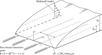
past a semi-infinite flat plate is considered. Superimposed on the flow are small vortical disturbances. Figure 1 shows a schematic of the flow domain. The interaction between these vortical disturbances and the laminar boundary layer above the flat plate gives rise to laminar streaks within the boundary layer. Quantities denoted by the superscript
 $\ast$
are dimensional, while quantities not marked by any symbol are non-dimensional. Velocities are scaled by
 $U_{\infty }^{\ast }$
, lengths by
 ${\it\lambda}_{z}^{\ast }$
(the spanwise wavelength of the free-stream disturbance), time by
 ${\it\lambda}_{z}^{\ast }/U_{\infty }^{\ast }$
and pressure by
 ${\it\rho}^{\ast }U_{\infty }^{\ast 2}$
, where
 ${\it\rho}^{\ast }$
is the density of the fluid. The Reynolds number is defined as
 $R_{{\it\lambda}}=U_{\infty }^{\ast }{\it\lambda}_{z}^{\ast }/{\it\nu}^{\ast }\gg 1$
, where
 ${\it\nu}^{\ast }$
is the kinematic viscosity of the fluid.
A schematic illustration of free-stream convected gusts interacting with the boundary layer above a spanwise oscillating plate.

The boundary-layer flow is made up of the streamwise (
 $x$
) velocity component
 $U^{\ast }$
, the wall-normal (
 $y$
) velocity component
 $V^{\ast }$
and the spanwise (
 $z$
) velocity component
 $\mathscr{W}^{\ast }$
. The wall oscillates sinusoidally in time along the spanwise direction, and the velocity components satisfy the no-slip and no-penetration conditions at the wall:
 $$\begin{eqnarray}\{U^{\ast },V^{\ast },\mathscr{W}^{\ast }\}=\{0,0,2\mathscr{W}_{m}^{\ast }\cos ({\it\omega}_{gsl}^{\ast }t^{\ast })\}=\{0,0,\mathscr{W}_{m}^{\ast }(\text{e}^{\text{i}{\it\omega}_{gsl}^{\ast }t^{\ast }}+\text{e}^{-\text{i}{\it\omega}_{gsl}^{\ast }t^{\ast }})\},\end{eqnarray}$$
where
 $2\mathscr{W}_{m}^{\ast }$
and
 ${\it\omega}_{gsl}^{\ast }$
are the amplitude and frequency of the wall oscillation, respectively. The non-dimensional Strouhal number
 $\overline{{\it\omega}}={\it\omega}_{gsl}/k_{x}=O(1)$
defines the frequency ratio, where
 $k_{x}$
is the frequency of the free-stream perturbation.
As for the stationary-wall case (LWG99), the free-stream velocity is represented by a uniform flow perturbed by small-amplitude vortical fluctuations of the convected gust type, i.e. disturbances that are passively convected by the uniform flow,
 $$\begin{eqnarray}\boldsymbol{u}=\hat{\boldsymbol{\imath }}+{\it\varepsilon}\hat{\boldsymbol{u}}^{\infty }\text{e}^{\text{i}(k_{x}x+k_{y}y+k_{z}z-k_{x}t)}+{\it\varepsilon}\hat{\boldsymbol{u}}^{\infty }\text{e}^{-\text{i}(k_{x}x+k_{y}y+k_{z}z-k_{x}t)},\end{eqnarray}$$
where
 $\hat{\boldsymbol{u}}^{\infty }=\{\hat{u} ^{\infty },\hat{v}^{\infty },{\hat{w}}^{\infty }\}$
and
 ${\it\varepsilon}\ll 1$
is a measure of the free-stream turbulence intensity. Attention is focused on free-stream disturbances with
 $k_{x}\ll k_{y}$
,
 $k_{x}\ll k_{z}$
and
 $k_{y}/k_{z}=O(1)$
, as experiments distinctly show that low-frequency disturbances are the most amplified within the boundary layer (Matsubara & Alfredsson Reference Matsubara and Alfredsson2001). The continuity equation links the perturbation velocity components and wavenumbers through
 $$\begin{eqnarray}k_{x}\hat{u} ^{\infty }+k_{y}\hat{v}^{\infty }+k_{z}{\hat{w}}^{\infty }=0,\end{eqnarray}$$
while scaling implies that
 $$\begin{eqnarray}\left|\hat{\boldsymbol{u}}^{\infty }\right|=\sqrt{(\hat{u} ^{\infty })^{2}+(\hat{v}^{\infty })^{2}+({\hat{w}}^{\infty })^{2}}=1.\end{eqnarray}$$
2.1. Base-flow equations
The boundary-layer base flow over which the perturbation flow evolves is formed by the interaction of the uniform flow
 $U_{\infty }^{\ast }$
with the spanwise oscillating wall and is independent of
 $z$
. Its velocity components along the
 $x$
,
 $y$
and
 $z$
directions are
 $U_{bl}$
,
 $V_{bl}$
and
 $\mathscr{W}_{gsl}$
, respectively. Upon substituting these velocity components into the Navier–Stokes equations, the
 $x$
- and
 $y$
-momentum equations decouple from the
 $z$
-momentum equation following the independence principle of Jones (Reference Jones1947). In the limit
 $\mathit{Re}_{{\it\lambda}}\gg 1$
,
 $(U_{bl},V_{bl})$
coincide with the classical laminar Blasius flow over a flat plate. In terms of the Blasius similarity coordinate
 $$\begin{eqnarray}{\it\eta}=\frac{y}{{\it\delta}_{bl}}=y\sqrt{\frac{\mathit{Re }_{{\it\lambda}}}{2x}},\end{eqnarray}$$
where
 ${\it\delta}_{bl}$
is the characteristic boundary-layer thickness, the Blasius flow is written as
 $$\begin{eqnarray}\{U_{bl},V_{bl}\}(x,{\it\eta})=\{F^{\prime }({\it\eta}),(2x\mathit{Re}_{{\it\lambda}})^{-1/2}[{\it\eta}F^{\prime }({\it\eta})-F({\it\eta})]\},\end{eqnarray}$$
where the prime indicates differentiation with respect to
 ${\it\eta}$
. The function
 $F({\it\eta})$
satisfies the Blasius equation
 $$\begin{eqnarray}F^{\prime \prime \prime }+FF^{\prime \prime }=0,\end{eqnarray}$$
subject to the boundary conditions
 $F(0)=0$
,
 $F^{\prime }(0)=0$
and
 $F\rightarrow {\it\eta}-{\it\beta}$
as
 ${\it\eta}\rightarrow \infty$
, where
 ${\it\beta}=1.217\dots$
.
Non-parallel terms, i.e. terms involving streamwise derivatives and the wall-normal velocity component
 $V_{bl}$
, are retained in the
 $z$
-momentum equation, which reads
 $$\begin{eqnarray}\frac{\partial \mathscr{W}_{gsl}}{\partial t}+U_{bl}\frac{\partial \mathscr{W}_{gsl}}{\partial x}+V_{bl}\frac{\partial \mathscr{W}_{gsl}}{\partial y}=\frac{1}{\mathit{Re}_{{\it\lambda}}}\left(\frac{\partial ^{2}\mathscr{W}_{gsl}}{\partial x^{2}}+\frac{\partial ^{2}\mathscr{W}_{gsl}}{\partial y^{2}}\right)\!.\end{eqnarray}$$
Equation (2.8) satisfies the boundary conditions
 $\mathscr{W}_{gsl}=2\mathscr{W}_{m}\cos (\overline{{\it\omega}}k_{x}t)$
at
 $y=0$
for
 $x>0$
and
 $\mathscr{W}_{gsl}\rightarrow 0$
as
 $y\rightarrow \infty$
. If the non-parallel terms were neglected, the base flow
 $\mathscr{W}_{gsl}$
would become independent of
 $x$
and would coincide with the classical Stokes layer above an oscillating wall (Batchelor Reference Batchelor1967, p. 192). In the following, the generalized Stokes layer described by (2.8) is referred to as GSL and the classical Stokes layer is denoted by CSL.
At this point it is appropriate to introduce the adopted scaling because it applies to the base flow and the perturbation flow. As shown by LWG99, the laminar streaks evolve over a distance that is much larger than the spanwise wavelength in the limit
 $\mathit{Re}_{{\it\lambda}}\gg 1$
. The
 $x$
coordinate is therefore scaled by
 ${\it\lambda}_{x}^{\ast }$
, the streamwise wavelength of the free-stream gust. This can be used as the representative scale of the downstream evolution of the Klebanoff modes because no wavelength-adjustment mechanism occurs, as in Goldstein (Reference Goldstein1983) for example. Time is rescaled by the gust period because this is the characteristic time of the streak unsteadiness. The new scaled variables are thus
 $\overline{x}=k_{x}x$
and
 $\overline{t}=k_{x}t$
. Laminar streaks are therefore observed at
 $\overline{x}=O(1)$
from the leading edge of the plate. It follows that the streamwise diffusion term in the spanwise base-flow equation (2.8) is
 $O(k_{x}/\mathit{Re}_{{\it\lambda}}\ll 1)$
and can be neglected, as it is asymptotically smaller than the other terms.
In the
 $(\overline{x},{\it\eta},\overline{t})$
coordinate system, (2.8) becomes
 $$\begin{eqnarray}\frac{\partial \mathscr{W}_{gsl}}{\partial \overline{t}}+F^{\prime }\frac{\partial \mathscr{W}_{gsl}}{\partial \overline{x}}-\frac{F}{2\overline{x}}\frac{\partial \mathscr{W}_{gsl}}{\partial {\it\eta}}=\frac{1}{2\overline{x}}\frac{\partial ^{2}\mathscr{W}_{gsl}}{\partial {\it\eta}^{2}},\end{eqnarray}$$
after use of (2.5), (2.6) and
 $\mathit{Re}_{{\it\lambda}}\gg 1$
. Equation (2.9) is linear and, consistently with (2.1), a solution is sought in the form
 $$\begin{eqnarray}\mathscr{W}_{gsl}(\overline{x},{\it\eta},\overline{t})=\frac{k_{x}}{k_{z}}W_{gsl}(\overline{x},{\it\eta},\overline{t})=\frac{k_{x}}{k_{z}}[W(\overline{x},{\it\eta})\text{e}^{\text{i}\overline{{\it\omega}}\overline{t}}+W^{\star }(\overline{x},{\it\eta})\text{e}^{-\text{i}\overline{{\it\omega}}\overline{t}}],\end{eqnarray}$$
where
 $^{\star }$
denotes the complex conjugate. The factor
 $k_{x}/k_{z}$
will be shown to be necessary to retain the terms synthesizing the effect of wall oscillations in the disturbance equations. Matching coefficients of
 $\text{e}^{\text{i}\overline{{\it\omega}}\overline{t}}$
in (2.9) leads to
 $$\begin{eqnarray}\text{i}\overline{{\it\omega}}W+F^{\prime }\frac{\partial W}{\partial \overline{x}}-\frac{F}{2\overline{x}}\frac{\partial W}{\partial {\it\eta}}=\frac{1}{2\overline{x}}\frac{\partial ^{2}W}{\partial {\it\eta}^{2}},\end{eqnarray}$$
which satisfies the free-stream boundary condition
 $W\rightarrow 0$
as
 ${\it\eta}\rightarrow \infty$
, and, at the wall,
 $W(\overline{x},0)=(k_{z}/k_{x})\mathscr{W}_{m}=W_{m}$
for
 $\overline{x}>0$
. Equation (2.11) is parabolic in
 $\overline{x}$
and therefore requires initial conditions for
 $\overline{x}\ll 1$
. These are derived in appendix A. Second-order implicit finite-difference schemes are employed to solve (2.11) (Cebeci Reference Cebeci2002).
2.2. Disturbance-flow equations
As LWG99 showed that
 $O({\it\varepsilon})$
free-stream perturbations lead to
 $O({\it\varepsilon}/k_{x})$
disturbances within the boundary layer, and because of the distinguished limit
 $k_{x}\mathit{Re}_{{\it\lambda}}=O(1)$
that emerges when the spanwise diffusion becomes comparable with the wall-normal diffusion, the condition for linearization for the boundary-layer disturbance equations is based upon a turbulent Reynolds number
 $r_{t}={\it\varepsilon}\mathit{Re}_{{\it\lambda}}\ll 1$
. The velocity and pressure fields are therefore expanded as
 $$\begin{eqnarray}\{U,V,\mathscr{W},P\}=\{U_{bl},V_{bl},\mathscr{W}_{gsl},-1/2\}(x,y,t)+r_{t}\{u,v,w,p\}(x,y,z,t).\end{eqnarray}$$
Following Gulyaev et al. (Reference Gulyaev, Kozlov, Kuznetsov, Mineev and Sekundov1989), LWG99 and Ricco (Reference Ricco2009), the disturbance velocities and pressure are further decomposed as
 $$\begin{eqnarray}\displaystyle \{u,v,w,p\} & = & \displaystyle Q\left\{\frac{k_{z}}{k_{x}}\overline{u},\,\sqrt{\frac{2\overline{x}k_{x}}{\mathit{Re}_{{\it\lambda}}}}\,\frac{k_{z}}{k_{x}}\,\overline{v},\,\overline{w},\,{\it\kappa}_{z}\sqrt{\frac{k_{x}}{\mathit{Re}_{{\it\lambda}}}}\,\overline{p}\right\}\nonumber\\ \displaystyle & & \displaystyle +\,Q^{(0)}\left\{\overline{u}^{(0)},\,\sqrt{\frac{2\overline{x}k_{x}}{\mathit{Re}_{{\it\lambda}}}}\,\overline{v}^{(0)},\,-\frac{k_{x}}{k_{z}}\,\overline{w}^{(0)},\,\frac{k_{x}}{\mathit{Re}_{{\it\lambda}}}\,\overline{p}^{(0)}\right\},\end{eqnarray}$$
where
 ${\it\kappa}_{z}=k_{z}/\sqrt{k_{x}\mathit{ Re }_{{\it\lambda}}}$
. The coefficients
 $Q=\text{i}{\it\kappa}_{z}^{2}({\hat{w}}^{\infty }+\text{i}k_{z}\hat{v}^{\infty }/{\it\Gamma})/k_{z}$
and
 $Q^{(0)}=\text{i}{\it\kappa}_{z}^{2}(\hat{u} ^{\infty }+\text{i}k_{x}\hat{v}^{\infty }/{\it\Gamma})/k_{z}$
, with
 ${\it\Gamma}=\sqrt{k_{x}^{2}+k_{z}^{2}}$
, are found through rapid distortion theory by ensuring the non-penetration of the vortical gusts near the leading edge of the plate.
Upon substituting (2.12) and (2.13) into the Navier–Stokes equations and by collecting terms of
 $O(r_{t})$
, it is found that the leading-order components in the core of the boundary layer, i.e.
 $\{\overline{u},\overline{v},\overline{w},\overline{p}\}$
, studied by LWG99, and the components that dominate the outer portion of the boundary layer, i.e.
 $\{\overline{u}^{(0)},\overline{v}^{(0)},\overline{w}^{(0)},\overline{p}^{(0)}\}$
, investigated by Ricco (Reference Ricco2009), satisfy the linearized unsteady boundary region (LUBR) equations, which, when modified to take into account the flow above a spanwise oscillating plate, take the form
 $$\begin{eqnarray}\displaystyle & & \displaystyle \displaystyle \frac{\partial \overline{u}}{\partial \overline{x}}-\frac{{\it\eta}}{2\overline{x}}\frac{\partial \overline{u}}{\partial {\it\eta}}+\frac{\partial \overline{v}}{\partial {\it\eta}}+\frac{1}{k_{z}}\frac{\partial \overline{w}}{\partial z}=0,\end{eqnarray}$$
 $$\begin{eqnarray}\displaystyle & & \displaystyle \displaystyle \frac{\partial \overline{u}}{\partial \overline{t}}+F^{\prime }\frac{\partial \overline{u}}{\partial \overline{x}}-\frac{{\it\eta}F^{\prime \prime }}{2\overline{x}}\overline{u}-\frac{F}{2\overline{x}}\frac{\partial \overline{u}}{\partial {\it\eta}}+F^{\prime \prime }\overline{v}+\frac{W_{gsl}}{k_{z}}\frac{\partial \overline{u}}{\partial z}\nonumber\\ \displaystyle & & \displaystyle \quad =\frac{1}{2\overline{x}}\frac{\partial ^{2}\overline{u}}{\partial {\it\eta}^{2}}+\frac{1}{k_{x}\mathit{Re}_{{\it\lambda}}}\frac{\partial ^{2}\overline{u}}{\partial z^{2}},\end{eqnarray}$$
 $$\begin{eqnarray}\displaystyle & & \displaystyle \displaystyle \frac{\partial \overline{v}}{\partial \overline{t}}+\frac{({\it\eta}F^{\prime })^{\prime }}{2\overline{x}}\overline{v}+F^{\prime }\frac{\partial \overline{v}}{\partial \overline{x}}-\frac{F}{2\overline{x}}\frac{\partial \overline{v}}{\partial {\it\eta}}+\frac{[F-{\it\eta}({\it\eta}F^{\prime })^{\prime }]}{(2\overline{x})^{2}}\overline{u}+\frac{W_{gsl}}{k_{z}}\frac{\partial \overline{v}}{\partial z}\nonumber\\ \displaystyle & & \displaystyle \quad =-\frac{1}{2\overline{x}}\frac{\partial \overline{p}}{\partial {\it\eta}}+\frac{1}{2\overline{x}}\frac{\partial ^{2}\overline{v}}{\partial {\it\eta}^{2}}+\frac{1}{k_{x}\mathit{Re}_{{\it\lambda}}}\frac{\partial ^{2}\overline{v}}{\partial z^{2}},\end{eqnarray}$$
 $$\begin{eqnarray}\displaystyle & & \displaystyle \displaystyle \frac{\partial \overline{w}}{\partial \overline{t}}+F^{\prime }\frac{\partial \overline{w}}{\partial \overline{x}}+\left(\frac{\partial W_{gsl}}{\partial \overline{x}}-\frac{{\it\eta}}{2\overline{x}}\frac{\partial W_{gsl}}{\partial {\it\eta}}\right)\overline{u}-\frac{F}{2\overline{x}}\frac{\partial \overline{w}}{\partial {\it\eta}}+\frac{\partial W_{gsl}}{\partial {\it\eta}}\overline{v}+\frac{W_{gsl}}{k_{z}}\frac{\partial \overline{w}}{\partial z}\nonumber\\ \displaystyle & & \displaystyle \quad =-\frac{k_{z}}{k_{x}\mathit{Re}_{{\it\lambda}}}\frac{\partial \overline{p}}{\partial z}+\frac{1}{2\overline{x}}\frac{\partial ^{2}\overline{w}}{\partial {\it\eta}^{2}}+\frac{1}{k_{x}\mathit{Re}_{{\it\lambda}}}\frac{\partial ^{2}\overline{w}}{\partial z^{2}}.\end{eqnarray}$$
 $\{\overline{u},\overline{v},\overline{w},\overline{p}\}$
, the leading-order terms inside the boundary layer. To account for the linear coupling between different modes, the solution can be expressed as a Fourier series in time
 $\overline{t}$
and the spanwise coordinate
 $z$
, with the form
 $$\begin{eqnarray}\{\overline{u},\overline{v},\overline{w},\overline{p}\}=\mathop{\sum }_{m,n=-\infty }^{\infty }\{\overline{u}^{[m,n]},\overline{v}^{[m,n]},\overline{w}^{[m,n]},\overline{p}^{[m,n]}\}\left(\overline{x},{\it\eta}\right)\text{e}^{\text{i}mk_{z}z+\text{i}n\overline{t}}.\end{eqnarray}$$
The Fourier coefficients satisfy the Hermitian conditions
 $$\begin{eqnarray}\{\overline{u}^{[-m,-n]},\overline{v}^{[-m,-n]},\overline{w}^{[-m,-n]},\overline{p}^{[-m,-n]}\}=\{\overline{u}^{[m,n]^{\star }},\overline{v}^{[m,n]^{\star }},\overline{w}^{[m,n]^{\star }},\overline{p}^{[m,n]^{\star }}\}.\end{eqnarray}$$
At this stage, attention is restricted to Strouhal numbers
 $\overline{{\it\omega}}=N$
, which is a strictly positive integer. This corresponds to a case in which the period of the gust is
 $N$
times the period of the wall oscillation. The extension of the formulation to wall oscillation periods that are integer multiples of the gust period is considered in § 4.3. Further extensions to rational and irrational Strouhal numbers are beyond the scope of this paper.
The first exponential term in (2.2) forces the
 $m=1$
and
 $n=-1$
mode in series (2.15), while its complex conjugate term in (2.2) forces the
 $m=-1$
and
 $n=1$
mode. All the other modes must decay at large distances from the plate, as the free-stream disturbance does not include these modes. Given a base flow of the form of (2.10), it is expedient to consider whether terms in the Fourier series are linked. Multiplying terms in the Fourier series with terms from the base-flow expansion of the form
 $\text{e}^{\pm \text{i}N\overline{t}}$
couples all the modes for a given
 $m$
value because a base flow of this form does not lead to spanwise coupling of modes. Modes with
 $m\neq \pm 1$
are not directly forced by the free-stream gust and are not connected to a forced term through the base flow. Therefore, the coefficients
 $\overline{u}^{[m,n]}$
,
 $\overline{v}^{[m,n]}$
,
 $\overline{w}^{[m,n]}$
and
 $\overline{p}^{[m,n]}$
equal zero if
 $m\neq \pm 1$
. The only non-zero modes are those that satisfy
 $m=\pm 1$
, and, given the Hermitian conditions (2.16), it is sufficient to consider the
 $m=1$
modes. In order to simplify the notation, these modes are subsequently denoted by
 $\{\overline{u}^{[n,1]},\overline{v}^{[n,1]},\overline{w}^{[n,1]},\overline{p}^{[n,1]}\}=\{\overline{u}^{[n]},\overline{v}^{[n]},\overline{w}^{[n]},\overline{p}^{[n]}\}$
. The
 $z$
dependence (contained in the
 $\text{e}^{\text{i}mk_{z}z}$
factor that multiplies every term) can also be eliminated.
For
 $N=1$
, the spanwise base flow introduces a modulation of the form
 $\text{e}^{\pm \text{i}\overline{t}}$
relating all the modes for which
 $m=\pm 1$
. However, for
 $N=2$
only the coefficients with
 $n$
odd are non-zero, while for larger
 $N$
even fewer terms are linked. This modulation produces terms involving
 $\text{e}^{\text{i}(n+N)\overline{t}}$
and
 $\text{e}^{\text{i}(n-N)\overline{t}}$
in the momentum equations. These terms can be written in the form
 $\text{e}^{\text{i}n\overline{t}}$
by means of a suitable redefinition of the dummy indexing variable. For instance, if
 ${\tilde{n}}$
is defined to satisfy
 ${\tilde{n}}=n-N$
, terms of the form
 $\overline{u}^{[n]}\text{e}^{\text{i}(n-N)\overline{t}}$
are transformed to
 $\overline{u}^{[{\tilde{n}}+N]}\text{e}^{\text{i}{\tilde{n}}\overline{t}}$
. All the remaining exponential terms can be written in the form
 $\text{e}^{\text{i}n\overline{t}}$
, while creating a linear coupling between the Fourier coefficients corresponding to different modes. This is numerically expedient and, for each
 $n$
, the Fourier coefficients satisfy the LUBR equations for the flow above a spanwise oscillating plate:
 $$\begin{eqnarray}\frac{\partial \overline{u}^{[n]}}{\partial \overline{x}}-\frac{{\it\eta}}{2\overline{x}}\frac{\partial \overline{u}^{[n]}}{\partial {\it\eta}}+\frac{\partial \overline{v}^{[n]}}{\partial {\it\eta}}+\text{i}\overline{w}^{[n]}=0,\end{eqnarray}$$
 $$\begin{eqnarray}\displaystyle & & \displaystyle \left(\text{i}n+{\it\kappa}_{z}^{2}-\frac{{\it\eta}F^{\prime \prime }}{2\overline{x}}\right)\overline{u}^{[n]}+F^{\prime }\frac{\partial \overline{u}^{[n]}}{\partial \overline{x}}-\frac{F}{2\overline{x}}\frac{\partial \overline{u}^{[n]}}{\partial {\it\eta}}-\frac{1}{2\overline{x}}\frac{\partial ^{2}\overline{u}^{[n]}}{\partial {\it\eta}^{2}}+F^{\prime \prime }\overline{v}^{[n]}\nonumber\\ \displaystyle & & \displaystyle \quad +\,\text{i}W\overline{u}^{[n-N]}+\text{i}W^{\star }\overline{u}^{[n+N]}=0,\end{eqnarray}$$
 $$\begin{eqnarray}\displaystyle & & \displaystyle \left(\text{i}n+{\it\kappa}_{z}^{2}+\frac{({\it\eta}F^{\prime })^{\prime }}{2\overline{x}}\right)\overline{v}^{[n]}+F^{\prime }\frac{\partial \overline{v}^{[n]}}{\partial \overline{x}}-\frac{F}{2\overline{x}}\frac{\partial \overline{v}^{[n]}}{\partial {\it\eta}}-\frac{1}{2\overline{x}}\frac{\partial ^{2}\overline{v}^{[n]}}{\partial {\it\eta}^{2}}\nonumber\\ \displaystyle & & \displaystyle \quad +\,\frac{[F-{\it\eta}({\it\eta}F^{\prime })^{\prime }]}{(2\overline{x})^{2}}\overline{u}^{[n]}+\frac{1}{2\overline{x}}\frac{\partial \overline{p}^{[n]}}{\partial {\it\eta}}+\text{i}W\overline{v}^{[n-N]}+\text{i}W^{\star }\overline{v}^{[n+N]}=0,\end{eqnarray}$$
 $$\begin{eqnarray}\displaystyle & & \displaystyle (\text{i}n+{\it\kappa}_{z}^{2})\overline{w}^{[n]}+F^{\prime }\frac{\partial \overline{w}^{[n]}}{\partial \overline{x}}-\frac{F}{2\overline{x}}\frac{\partial \overline{w}^{[n]}}{\partial {\it\eta}}-\frac{1}{2\overline{x}}\frac{\partial ^{2}\overline{w}^{[n]}}{\partial {\it\eta}^{2}}+\text{i}{\it\kappa}_{z}^{2}\overline{p}^{[n]}\nonumber\\ \displaystyle & & \displaystyle \quad +\,\left(\frac{\partial W}{\partial \overline{x}}-\frac{{\it\eta}}{2\overline{x}}\frac{\partial W}{\partial {\it\eta}}\right)\overline{u}^{[n-N]}+\frac{\partial W}{\partial {\it\eta}}\overline{v}^{[n-N]}+\text{i}W\overline{w}^{[n-N]}\nonumber\\ \displaystyle & & \displaystyle \quad +\,\left(\frac{\partial W^{\star }}{\partial \overline{x}}-\frac{{\it\eta}}{2\overline{x}}\frac{\partial W^{\star }}{\partial {\it\eta}}\right)\overline{u}^{[n+N]}+\frac{\partial W^{\star }}{\partial {\it\eta}}\overline{v}^{[n+N]}+\text{i}W^{\star }\overline{w}^{[n+N]}=0.\end{eqnarray}$$
 $\overline{{\it\omega}}=N$
. This is a system of parabolic equations for each
 $\{\overline{u}^{[n]},\overline{v}^{[n]},\overline{w}^{[n]},\overline{p}^{[n]}\}$
. The no-slip boundary conditions are applied at the wall, while the free-stream boundary conditions and the initial conditions for
 $\overline{x}\ll 1$
are found in appendix B. The numerical procedures are described in appendix C.
3. Spanwise base flow
The spanwise base flow is now analysed and compared with the CSL, i.e. the flow obtained by sinusoidal oscillations of a flat plate below a quiescent fluid. The differences in the perturbation flow field arising from the use of the asymptotically correct GSL and the CSL are discussed.
In the coordinate system
 $(\overline{x},{\it\eta})$
, the CSL solution (Batchelor Reference Batchelor1967, p. 192) for the flow above an oscillating plate has the form
 $$\begin{eqnarray}\mathscr{W}_{csl}=2\mathscr{W}_{m}\exp \!\left(-\sqrt{\overline{{\it\omega}}\,\overline{x}}\,{\it\eta}\right)\cos \!\left(\overline{{\it\omega}}\,\overline{t}-\sqrt{\overline{{\it\omega}}\,\overline{x}}\,{\it\eta}\right).\end{eqnarray}$$
The CSL has uniform thickness in the streamwise direction. However, once scaled by the Blasius wall-normal coordinate
 ${\it\eta}$
, the CSL thickness decays due to the exponential dependence on
 $\sqrt{\overline{x}}$
.
3.1. Large-
 $\overline{x}$
and high-frequency spanwise base flows

Upon defining a new coordinate
 $\hat{x}=N\overline{x}={\it\omega}_{gsl}^{\ast }x^{\ast }/U_{\infty }^{\ast }$
(i.e. by scaling through the streamwise distance travelled by a free-stream fluid particle during one plate oscillation period), the spanwise base-flow (2.11) becomes
 $$\begin{eqnarray}\text{i}W+F^{\prime }\frac{\partial W}{\partial \hat{x}}-\frac{F}{2\hat{x}}\frac{\partial W}{\partial {\it\eta}}=\frac{1}{2\hat{x}}\frac{\partial ^{2}W}{\partial {\it\eta}^{2}}.\end{eqnarray}$$
Large values of
 $\hat{x}$
correspond to either large downstream distances at fixed Strouhal number or, at a fixed downstream distance, to a sequence of flows for which the wall oscillates with increasing frequency. To analyse the flow behaviour for
 $\hat{x}$
large, a Wentzel–Kramers–Brillouin–Jeffreys (WKBJ) solution of (3.2) is sought with the form
 $$\begin{eqnarray}W=\overline{W}(\hat{x},{\it\eta})\text{e}^{-(2\hat{x})^{1/2}{\it\Theta}({\it\eta})},\end{eqnarray}$$
following the analysis of LWG99 for the edge layer. Matching coefficients of powers of
 $\hat{x}$
gives
 $$\begin{eqnarray}[{\it\Theta}^{\prime }({\it\eta})]^{2}=\text{i}\end{eqnarray}$$
at leading order. The permissible solution, which satisfies
 $W(\hat{x},0)=W_{m}$
and decays for large
 ${\it\eta}$
, is
 $$\begin{eqnarray}{\it\Theta}({\it\eta})=\frac{(1+\text{i}){\it\eta}}{\sqrt{2}}.\end{eqnarray}$$
Matching coefficients at
 $O(\hat{x}^{-1/2})$
gives
 $$\begin{eqnarray}\overline{W}^{\prime }=(F^{\prime }{\it\eta}-F)\frac{\overline{W}}{2}.\end{eqnarray}$$
The large-
 $\hat{x}$
solution of the GSL flow is
 $$\begin{eqnarray}\left.\mathscr{W}_{gsl}\right|_{\hat{x}\gg 1}=\frac{\mathscr{W}_{m}F^{\prime \prime }({\it\eta})}{F^{\prime \prime }(0)}\exp \!\left(\frac{F{\it\eta}}{2}\right)\exp [-\hat{x}^{1/2}(1+\text{i}){\it\eta}]\exp (\text{i}N\overline{t})+\text{c.c.},\end{eqnarray}$$
where
 $\text{c.c}$
. indicates the complex conjugate. For
 $\mathscr{W}_{gsl}$
to be
 $O(1)$
, the exponent in the second exponential function,
 $\hat{x}^{1/2}(1+\text{i}){\it\eta}$
, must be
 $O(1)$
, and therefore, for
 $\hat{x}\gg 1$
, it is only significant when
 ${\it\eta}\ll 1$
. In this limit the exponent of the first exponential function is small and, on returning to dimensional variables, the remaining terms give
 $$\begin{eqnarray}\left.\mathscr{W}_{gsl}\right|_{\hat{x}\gg 1}\sim \mathscr{W}_{m}\exp \!\left[-(1+\text{i})\sqrt{\frac{{\it\omega}_{gsl}^{\ast }}{2{\it\nu}^{\ast }}}y^{\ast }\right]\exp (\text{i}{\it\omega}_{gsl}^{\ast }t^{\ast })+\text{c.c}.\end{eqnarray}$$
Expression (3.8) matches the CSL solution for the flow above an oscillating plate. Therefore, it is proven that the GSL flow approaches the CSL flow as
 $\hat{x}$
increases.
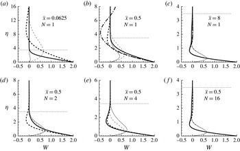
This is verified in figure 2, via comparison between the GSL numerical solution of (2.11) (solid lines) and the CSL analytical solution (3.1) (dashed lines). The dotted lines indicate the Blasius boundary-layer thickness, here defined as the
 ${\it\eta}$
location at which the streamwise velocity is equal to
 $0.99U_{\infty }^{\ast }$
. The top row illustrates the evolution in
 $\overline{x}$
of both types of Stokes layers for
 $N=1$
. For small
 $\overline{x}$
, the CSL initially penetrates much further into the flow than both the GSL and the Blasius boundary layer. At
 $\overline{x}=0.5$
, the ratio between the CSL thickness and the GSL thickness is smaller than at
 $\overline{x}=0.0625$
and the CSL is still thicker than the Blasius layer. Further downstream, the difference between the two Stokes profiles decreases and the spanwise layers occupy a smaller and smaller proportion of the Blasius boundary layer as
 $\overline{x}$
grows. For large
 $\overline{x}$
(
 $\overline{x}=8$
,
 $N=1$
, figure 2
c), the differences between the GSL and the CSL become very small, as non-parallel flow effects attenuate as
 $\overline{x}$
increases. This matches the WKBJ prediction.
GSL profiles (solid lines) and CSL profiles (dashed lines). The thick lines correspond to
 $t=0$
, while the thin lines correspond to a
 ${\rm\pi}/2$
phase shift. (a–c) Profiles with increasing
 $\overline{x}$
and
 $N=1$
; (d–f) profiles with increasing
 $N$
and
 $\overline{x}=0.5$
. The Blasius boundary-layer thickness, here defined as the
 ${\it\eta}$
location at which
 $U_{bl}^{\ast }=0.99U_{\infty }^{\ast }$
(dotted lines), and the WKBJ solution (3.7) at
 $t=0$
(dash-dotted lines in (b) and (c)) are also shown.

The lower row shows the base-flow profiles at fixed
 $\overline{x}=0.5$
, in a sequence of flows for which
 $N$
increases. As predicted by the WKBJ theory, the discrepancies between the GSL and the CSL decrease as the oscillation frequency grows. Figure 2(c, f) shows two cases in which
 $\hat{x}=N\overline{x}=8$
. The profiles are identical up to very small numerical differences, which have absolute value less than
 $10^{-2}$
. This further justifies the definition of a new streamwise coordinate
 $\hat{x}=N\overline{x}\gg 1$
for the WKBJ analysis. Figure 2(b,c) also confirms the convergence of the GSL profile to the WKBJ solution (3.7), shown by dash-dotted lines.
The confinement of the GSL within the Blasius boundary layer occurs at every
 $\overline{x}$
and is a distinguished feature of this flow. This is markedly different from the CSL, which is much thicker than the Blasius layer at small
 $\overline{x}$
, as shown in figure 2(a). The GSL remains confined within the Blasius boundary layer because viscous effects in the spanwise momentum equation are now balanced by the steady convection terms. This is different from the case of viscous effects being balanced by the unsteady convection term as in the classical problem studied by Rayleigh (see Schlichting & Gersten Reference Schlichting and Gersten2001, p. 126), which leads to unbounded growth of the boundary layer over time. To prove that, sufficiently far upstream, the GSL thickness
 ${\it\delta}_{gsl}$
is comparable with
 ${\it\delta}_{bl}$
, the Blasius boundary-layer thickness, in the spanwise momentum equation, it is sufficient to scale
 $y^{\ast }$
by
 ${\it\delta}_{gsl}^{\ast }$
and
 $x^{\ast }$
by a length
 $L^{\ast }$
,
 ${\it\nu}^{\ast }/U_{\infty }^{\ast }\ll L^{\ast }\ll U_{\infty }^{\ast }/k_{x}^{\ast }$
, i.e. large enough to be able to neglect the streamwise viscous diffusion effects and small enough to ensure
 $\overline{x}\ll 1$
. This shows that
 $$\begin{eqnarray}{\it\delta}_{gsl}^{\ast }\sim {\it\delta}_{bl}^{\ast }\sim \left(\frac{L^{\ast }{\it\nu}^{\ast }}{U_{\infty }^{\ast }}\right)^{1/2},\end{eqnarray}$$
and that the unsteady term is negligible at leading order.
4. Linearized disturbance flow
Linear disturbances above a spanwise oscillating plate are now investigated with the aim of determining the conditions that produce reductions in the streak energy. To reduce the parameter space, only free-stream disturbances with
 ${\it\kappa}_{y}={\it\kappa}_{z}$
are considered (denoted subsequently by
 ${\it\kappa}$
), where
 ${\it\kappa}_{y}$
is the scaled wall-normal wavenumber defined in appendix B after (B 1).
At each streamwise and wall-normal position the root mean square (r.m.s.) value of the streamwise velocity can be reconstructed from the streamwise Fourier coefficients as
 $$\begin{eqnarray}\overline{u}_{rms}(\overline{x},{\it\eta})=\left[2\mathop{\sum }_{n=-\infty \atop n\neq 0}^{\infty }\left|\overline{u}^{[n]}(\overline{x},{\it\eta})\right|^{2}\right]^{1/2},\end{eqnarray}$$
where the factor of 2 follows from the Hermitian condition. The streak energy is computed by integrating the square of the r.m.s. velocity over the wall-normal and streamwise directions as follows:
 $$\begin{eqnarray}E=\int _{0}^{\infty }\int _{0}^{\infty }\left|\overline{u}_{rms}\!\left(\overline{x},{\it\eta}\right)\right|^{2}\text{d}\overline{x}\,\text{d}{\it\eta}.\end{eqnarray}$$
Above a stationary plate, all the streak energy is contained within the forced mode. As
 $W_{m}$
increases, unforced modes in the Fourier series become coupled to the forced one, and energy is transferred from the forced modes to the adjacent modes in the Fourier series. Consequently, the energy contained in coupled modes other than the forced one increases with
 $W_{m}$
, while the energy contained within the forced mode falls.
The change in streak intensity for
 ${\it\kappa}=1$
,
 $W_{m}=8$
and
 $N=1$
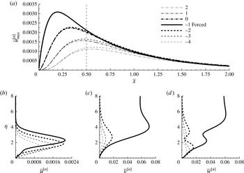
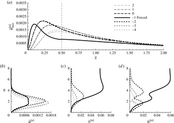
is shown in figure 3. Figure 3(a) shows the streamwise growth and decay of the maximum streamwise velocity
 $$\begin{eqnarray}\overline{u}_{max}^{[n]}\!\left(\overline{x}\right)=\max _{{\it\eta}}\!\left\{\overline{u}^{[n]}\!\left(\overline{x},{\it\eta}\right)\right\},\end{eqnarray}$$
associated with the
 $n$
th mode. The forced mode is indicated by a solid line, while dashed and dot-dashed lines show the lower and higher indexed unforced modes, respectively. Across all the modes, the maximum velocity is obtained in the forced mode, while the other modes show lower and lower energies as the distance in Fourier space from the forced mode increases. The
 $\overline{x}$
position of the overall maximum velocity of each mode moves downstream as the mode index increases relatively to the forced mode. These effects are due to the gradual energy transfer to the unforced modes over increasing
 $\overline{x}$
, compared to direct energy input into the forced mode from the free stream.
(a) Streamwise evolution of
 $\overline{u}_{max}^{[n]}\!\left(\overline{x}\right)$
for the forced mode
 $n=-1$
and six adjacent modes, when the spanwise base flow is given by a GSL with
 $W_{m}=8$
. (b–d) Corresponding profiles for
 $\overline{u}^{[n]}$
,
 $\overline{v}^{[n]}$
and
 $\overline{w}^{[n]}$
modes with negative index at
 $\overline{x}=0.5$
.

Figure 3(b–d) shows wall-normal profiles of the forced mode and the next three largest unforced modes with negative index for the
 $\overline{u}$
,
 $\overline{v}$
and
 $\overline{w}$
profiles at
 $\overline{x}=0.5$
. The modes at the same relative distance in Fourier space from the forced mode have very similar shape and therefore modes with zero or positive index are not shown for clarity. The maximum
 $\overline{u}$
moves closer to the wall as the distance in Fourier space relative to the forced mode increases. Only the forced
 $\overline{v}$
and
 $\overline{w}$
modes are non-zero in the far field, which follows from the free-stream boundary conditions (B 1).
4.1. Laminar streaks in classical and generalized Stokes layer spanwise base flows
The aim of this section is to compare the streak dynamics computed by the use of the GSL with the streak evolution when the CSL is employed as spanwise base flow. As outlined in § 1, this study is motivated by the results of Hack & Zaki (Reference Hack and Zaki2012), who utilized the CSL to alter the laminar streaks.
The maximum streamwise r.m.s. velocity at each
 $\overline{x}$
is denoted by
 $$\begin{eqnarray}\overline{u}_{max}\!\left(\overline{x}\right)=\max _{{\it\eta}}\left\{\overline{u}_{rms}\!\left(\overline{x},{\it\eta}\right)\right\},\end{eqnarray}$$
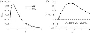
and is shown in figure 4(a) for a GSL and a CSL for
 $W_{m}=8$
,
 ${\it\kappa}=1$
and
 $N=1$
. On first inspection, these profiles suggest that the streaks generated by the two spanwise Stokes layers are rather similar, with the percentage relative error,
 $$\begin{eqnarray}\mathscr{E}\,(\%)=100\left(\frac{E_{gsl}-E_{csl}}{E_{gsl}}\right),\end{eqnarray}$$
between the two flows being 1.8 %. In this case the GSL streaks have more energy than the CSL streaks. The CSL and GSL streaks have the same intensity for
 ${\it\kappa}\approx 0.9$
, while for
 ${\it\kappa}$
smaller than this value the CSL calculation overpredicts the energy. For
 ${\it\kappa}>0.9$
, the CSL gives an underprediction of the energy, which reaches its maximum when
 ${\it\kappa}\approx 2.7$
. For larger
 ${\it\kappa}$
values the CSL streak energy approaches the GSL streak energy. All these cases are for
 $N=1$
, as the WKBJ analysis of § 3 indicates that the GSL tends to the CSL as
 $N$
increases.
(a) Evolution of
 $\overline{u}_{max}$
with
 $W_{m}=8$
and
 ${\it\kappa}=1$
for a GSL and a CSL and (b) the percentage error in the total streak energy versus
 ${\it\kappa}$
if the CSL is used instead of the GSL. The case presented in (a) is circled in (b).

The laminar streaks in the CSL case are further investigated in figure 5. The same case presented in figure 3 (
 $N=1$
,
 ${\it\kappa}=1$
,
 $W_{m}=8$
) is shown, the only difference being the use of the CSL instead of the GSL. Although the
 $\overline{u}_{rms}$
profiles, shown in figure 4, are similar and only have a 1.8 % difference in total streak energy, the profiles of the individual modes in figures 3 and 5 are notably different. When the CSL is used, the maximum velocity of the forced mode is less than two-thirds of the equivalent velocity generated when the GSL is used. This is because the CSL is thicker than the GSL for
 $\overline{x}\ll 1$
(refer to figure 2), and consequently the energy contained in the forced mode is more rapidly transferred to the other Fourier modes.
As figure 3, but showing the disturbance evolution when interacting with a CSL rather than a GSL.

The changes in the relative error in streak energies are not consistent with what might be expected from the analysis on the large-
 $\overline{x}$
behaviour of the spanwise base flow, studied in § 3.1. Streaks with small
 ${\it\kappa}$
values are less attenuated by viscous effects and therefore persist over larger
 $\overline{x}$
. Far downstream the difference between the GSL and CSL decreases, so one might expect the difference in the streak energy to diminish, too. This is not supported by figure 4, which shows that significant relative errors result from overprediction of streak energy at small
 ${\it\kappa}$
when the CSL is used. This indicates that the difference in streak energies is accrued at smaller
 $\overline{x}$
.
The largest differences between the GSL- and CSL-driven mode profiles, shown at the bottom of figures 3 and 5, are observed in the
 $\overline{u}$
component, with the forced mode being particularly affected. This is the velocity component that dominates the boundary-layer dynamics. The differences between the
 $\overline{v}$
and the
 $\overline{w}$
profiles are smaller. When the CSL is employed, the forced mode no longer has the largest streamwise velocity, while the monotonic decay of the maxima relative to the forced mode in the GSL case is no longer detected.
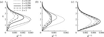
A final comparison of the streamwise velocity profiles is shown in figure 6, where the forced mode in (a) the GSL case, (b) the CSL case and (c) the stationary-wall case are shown at several
 $\overline{x}$
positions. In comparison to the stationary-wall case, the maxima of the GSL-induced forced mode occur at larger wall-normal distances, while the wall shear stress associated with the GSL modes is also reduced. These changes are also observed when streamwise velocity profiles with steady spanwise wall forcing are compared with those above a stationary plate (see Ricco Reference Ricco2011, figure 9). Comparisons with the CSL-induced modes are less conclusive, as these profiles often have multiple local velocity maxima, which may be located at a lower or higher wall-normal position with respect to the corresponding maxima in the stationary-wall case.
Wall-normal distributions of the forced streamwise velocity mode
 $\overline{u}^{[-1]}$
at a range of
 $\overline{x}$
for (a) a GSL, (b) a CSL and (c) a stationary-wall case. In all cases
 ${\it\kappa}=1$
, while
 $W_{m}=8$
and
 $N=1$
where spanwise wall forcing is present.

(a) The streamwise evolution of
 $\overline{u}_{max}\!\left(\overline{x}\right)$
for
 $N=1$
,
 ${\it\kappa}=1$
and a range of
 $W_{m}$
, and (b) the corresponding percentage energy reductions compared to a stationary plate.

4.2. Variation with plate oscillation amplitude
The energy contained in the forced mode with GSL forcing falls as
 $W_{m}$
grows, while the energy of the unforced modes increases. Therefore, it is opportune to discern whether the total energy rises or falls as
 $W_{m}$
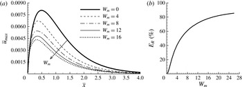
changes. The evolution of
 $\overline{u}_{max}$
is shown in figure 7(a) for a free-stream perturbation with
 ${\it\kappa}=1$
,
 $N=1$
and a range of
 $W_{m}$
. The energy falls monotonically as
 $W_{m}$
increases, while the position of the global maximum velocity moves towards
 $\overline{x}=0$
. This is reflected in figure 7(b), which shows the percentage energy reduction compared to a stationary plate,
 $$\begin{eqnarray}E_{R}\,(\%)=100\left(\frac{E_{stat}-E_{oscil}}{E_{stat}}\right)\!,\end{eqnarray}$$
as
 $W_{m}$
increases. The energy reduction with increasing
 $W_{m}$
indicates that the energy lost from the forced mode above an oscillating plate is larger than the energy transferred to the adjacent unforced modes by the plate oscillations. Therefore, this can potentially be a successful method for delaying transition in laminar boundary layers.
The energy reductions compare favourably with those obtained by Ricco (Reference Ricco2011, figure 8) for the response of laminar streaks to steady sinusoidal spanwise wall oscillations. Energy reductions were found to increase with the amplitude of the steady wall oscillations. In the current study, the amplitude of the spanwise forcing differs by a factor
 $2k_{x}/k_{z}$
from that earlier study. In the present notation, a steady wall oscillation of amplitude
 $W_{m}=15.7$
, for example, corresponds to an energy reduction of 89 % compared to a stationary plate when
 ${\it\kappa}=1$
. This value is larger than the energy reductions obtained herein. However, the maximum energy reductions of Ricco (Reference Ricco2011) were optimized with respect to the streamwise wavelength of the sinusoidal forcing, which makes like-for-like quantitative comparison difficult, as the equivalent optimization (with respect to
 $N$
) has not been carried out.
4.3. Variation with plate oscillation frequency
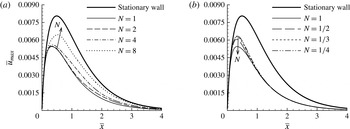
Figure 8(a) shows the evolution of
 $\overline{u}_{max}$
for
 ${\it\kappa}=1$
,
 $W_{m}=8$
and integer values of
 $N\geqslant 1$
. The formulation presented so far is restricted to integer values of
 $N$
, corresponding to
 $N$
plate oscillations per free-stream gust oscillation. For increasing
 $N$
values, the maximum streamwise velocity increases, while the position of the maximum moves slightly downstream. Increments in streamwise velocity from the
 $N=1$
streak are first noted in the region of streak decay, and move towards the location of maximum velocity as
 $N$
increases. There is a sizeable energy reduction even for
 $N=8$
. For
 $N>1$
the non-zero modes spread out, leaving
 $N-1$
zero-valued coefficients between each non-zero mode. For computational expediency, only the non-zero modes are calculated.
The streamwise evolution of
 $\overline{u}_{max}\!\left(\overline{x}\right)$
for
 ${\it\kappa}=1$
,
 $W_{m}=8$
and a range of
 $N$
.

The formulation can be generalized to consider plate oscillations that take longer than free-stream gust oscillations by introducing a new scaled time
 $\hat{t}=\overline{{\it\omega}}\overline{t}$
. In particular, if there exists an integer
 $\hat{N}$
such that
 $\overline{{\it\omega}}=\hat{N}^{-1}$
, these cases can be explored by taking
 $N=1$
in (2.17), and
 $j=-\hat{N}$
in (B 1) and (B 4). This configuration corresponds to
 $\hat{N}$
free-stream gust oscillations over one period of wall oscillation.
Cases for
 $N\leqslant 1$
with increasing
 $\hat{N}$
values are shown in figure 8(b). Larger maxima are observed for decreasing
 $N$
. The profiles remain largely unchanged when the streaks decay, with the increases being largely localized about the point of maximum velocity. Only modes with
 $-N_{f}\leqslant n\leqslant N_{f}$
are calculated, where
 $N_{f}$
is the maximum number of modes of the truncated series, as discussed in appendix C. For larger
 $\hat{N}$
values, it was not possible to obtain converged solutions for computationally practical values of
 $N_{f}$
, as the forced mode becomes closer to the edge of the band of calculated modes.
For
 ${\it\kappa}=1$
and
 $W_{m}=8$
, the lowest streamwise streak velocities are obtained for
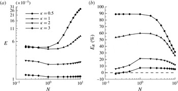
 $N=1$
. This is confirmed in figure 9(a), which shows energies for a range of
 ${\it\kappa}$
values and
 $W_{m}=8$
. For increasing
 ${\it\kappa}$
, the Strouhal number
 $N$
associated with the minimum total energy increases slightly. For larger
 ${\it\kappa}$
values, the range of energies narrows. The corresponding energy reductions are shown in figure 9(b). These indicate that the wall motion is less effective at reducing the energy for larger
 ${\it\kappa}$
values, and in some cases (
 ${\it\kappa}=3$
and
 $N<1/4$
), the streak energy grows.
(a) The total energies for
 $W_{m}=8$
and a range of
 ${\it\kappa}$
values and (b) the corresponding energy reductions.

4.4. Variation with free-stream gust properties
The disturbance profile is strongly affected by changes in the free-stream gust properties, with the streamwise extent of the disturbances being reduced (increased) as
 ${\it\kappa}$
increases (decreases), causing more (less) viscous dissipation. For streaks above a stationary plate with large
 ${\it\kappa}$
, LWG99 showed that the steady boundary region equations describe the streak dynamics and all the scaled disturbance profiles collapse on top of one another for large
 ${\it\kappa}$
. The equivalent scaled disturbances above a spanwise oscillating plate are now investigated.
4.4.1. Large
${\it\kappa}$
and
$N=O(1)$
scaling


Motivated by the scaling of LWG99, scaled velocity and pressure Fourier modes for
 ${\it\kappa}\gg 1$
are proposed in the form
 $$\begin{eqnarray}\{\overline{u}^{[n]},\overline{v}^{[n]},\overline{w}^{[n]},\overline{p}^{[n]}\}=\{\widetilde{u}^{[n]},{\it\kappa}^{2}\widetilde{v}^{[n]},{\it\kappa}^{2}\widetilde{w}^{[n]},{\it\kappa}^{2}\widetilde{p}^{[n]}\}\!\left(\widetilde{x},{\it\eta}\right),\end{eqnarray}$$
where
 $\widetilde{x}={\it\kappa}^{2}\overline{x}$
. Note that this scaling differs by a multiplicative factor
 ${\it\kappa}^{2}$
from the earlier scaling proposed by LWG99 (refer to their equations 5.32–5.34). This difference is accounted for by the extra factor
 ${\it\kappa}_{z}^{2}$
present in
 $Q$
in (2.13).
If this scaling is applied, the terms arising from time derivatives and the terms involving the spanwise base flow are
 $O({\it\kappa}^{-2})$
smaller than the remaining steady terms. Consequently, if this scaling is applied without additionally rescaling the spanwise base flow, the inter-mode coupling vanishes in the large-
 ${\it\kappa}$
limit. The unforced modes have zero disturbance velocities, while the behaviour of the forced mode is given by the linearized steady boundary region equations of LWG99 for disturbances above a stationary plate. In this case, the large-
 ${\it\kappa}$
scaling analysis of LWG99 applies directly to the forced mode, with the scaled streamwise disturbance velocities tending to the LWG99 large-
 ${\it\kappa}$
profiles.
To retain interactions between different modes for large
 ${\it\kappa}$
, it is necessary to scale the spanwise base flow, i.e.
 $\widetilde{W}=W{\it\kappa}^{-2}$
. If attention is restricted to
 $N=O(1)$
, as terms involving time derivatives appear at
 $O({\it\kappa}^{-2})$
, (2.9) simplifies to
 $$\begin{eqnarray}F^{\prime }\frac{\partial \widetilde{W}}{\partial \widetilde{x}}-\frac{F}{2\widetilde{x}}\frac{\partial \widetilde{W}}{\partial {\it\eta}}=\frac{1}{2\widetilde{x}}\frac{\partial ^{2}\widetilde{W}}{\partial {\it\eta}^{2}},\end{eqnarray}$$
subject to
 $\widetilde{W}=\widetilde{W}_{m}$
for
 $\widetilde{x}>0$
,
 ${\it\eta}=0$
. With sinusoidal rather than uniform spanwise wall forcing, an equation of this form also governs the steady spanwise base flow above a wall with steady spanwise forcing (Ricco Reference Ricco2011, equation 5). However, in the current case, the spanwise base flow remains time-dependent, as the actual velocity is reconstructed using (2.10). The problem of uniform spanwise motion beneath a Blasius boundary layer was previously studied by Fang & Lee (Reference Fang and Lee2009), and therefore the solution of (4.8) can be expressed as
 $$\begin{eqnarray}\widetilde{W}=\widetilde{W}_{m}(1-F^{\prime }),\end{eqnarray}$$
confirming that the fully developed spanwise boundary layer has a comparable wall-normal extent as the Blasius boundary layer near the leading edge. The spanwise flow (4.9) exactly matches the leading-order small-
 $\overline{x}$
behaviour (A 3) of the full unsteady problem.
In the limit
 ${\it\kappa}\gg 1$
, the solution of (4.8) becomes strictly real-valued and hence the perturbations satisfy LUBR equations of the form
 $$\begin{eqnarray}\frac{\partial \widetilde{u}^{[n]}}{\partial \widetilde{x}}-\frac{{\it\eta}}{2\widetilde{x}}\frac{\partial \widetilde{u}^{[n]}}{\partial {\it\eta}}+\frac{\partial \widetilde{v}^{[n]}}{\partial {\it\eta}}+\text{i}\widetilde{w}^{[n]}=0,\end{eqnarray}$$
 $$\begin{eqnarray}\displaystyle & & \displaystyle \left(1-\frac{{\it\eta}F^{\prime \prime }}{2\widetilde{x}}\right)\widetilde{u}^{[n]}+F^{\prime }\frac{\partial \widetilde{u}^{[n]}}{\partial \widetilde{x}}-\frac{F}{2\widetilde{x}}\frac{\partial \widetilde{u}^{[n]}}{\partial {\it\eta}}-\frac{1}{2\widetilde{x}}\frac{\partial ^{2}\widetilde{u}^{[n]}}{\partial {\it\eta}^{2}}+F^{\prime \prime }\widetilde{v}^{[n]}\nonumber\\ \displaystyle & & \displaystyle \qquad +\,\text{i}\widetilde{W}\widetilde{u}^{[n-N]}+\text{i}\widetilde{W}\widetilde{u}^{[n+N]}=0,\end{eqnarray}$$
 $$\begin{eqnarray}\displaystyle & & \displaystyle \left(1+\frac{({\it\eta}F^{\prime })^{\prime }}{2\widetilde{x}}\right)\widetilde{v}^{[n]}+F^{\prime }\frac{\partial \widetilde{v}^{[n]}}{\partial \widetilde{x}}-\frac{F}{2\widetilde{x}}\frac{\partial \widetilde{v}^{[n]}}{\partial {\it\eta}}-\frac{1}{2\widetilde{x}}\frac{\partial ^{2}\widetilde{v}^{[n]}}{\partial {\it\eta}^{2}}\nonumber\\ \displaystyle & & \displaystyle \qquad +\,\frac{(F-{\it\eta}({\it\eta}F^{\prime })^{\prime })}{(2\widetilde{x})^{2}}\widetilde{u}^{[n]}+\frac{1}{2\widetilde{x}}\frac{\partial \widetilde{p}^{[n]}}{\partial {\it\eta}}+\text{i}\widetilde{W}\widetilde{v}^{[n-N]}+\text{i}\widetilde{W}\widetilde{v}^{[n+N]}=0,\end{eqnarray}$$
 $$\begin{eqnarray}\displaystyle & & \displaystyle \widetilde{w}^{[n]}+F^{\prime }\frac{\partial \widetilde{w}^{[n]}}{\partial \widetilde{x}}-\frac{F}{2\widetilde{x}}\frac{\partial \widetilde{w}^{[n]}}{\partial {\it\eta}}-\frac{1}{2\widetilde{x}}\frac{\partial ^{2}\widetilde{w}^{[n]}}{\partial {\it\eta}^{2}}+\text{i}\widetilde{p}^{[n]}\nonumber\\ \displaystyle & & \displaystyle \qquad +\,\left(\frac{\partial \widetilde{W}}{\partial \widetilde{x}}-\frac{{\it\eta}}{2\widetilde{x}}\frac{\partial \widetilde{W}}{\partial {\it\eta}}\right)\widetilde{u}^{[n-N]}+\frac{\partial \widetilde{W}}{\partial {\it\eta}}\widetilde{v}^{[n-N]}+\text{i}\widetilde{W}\widetilde{w}^{[n-N]}\nonumber\\ \displaystyle & & \displaystyle \qquad +\,\left(\frac{\partial \widetilde{W}}{\partial \widetilde{x}}-\frac{{\it\eta}}{2\widetilde{x}}\frac{\partial \widetilde{W}}{\partial {\it\eta}}\right)\widetilde{u}^{[n+N]}+\frac{\partial \widetilde{W}}{\partial {\it\eta}}\widetilde{v}^{[n+N]}+\text{i}\widetilde{W}\widetilde{w}^{[n+N]}=0.\end{eqnarray}$$
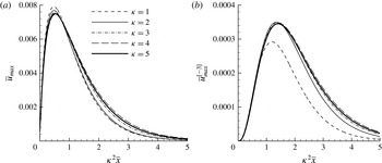
 ${\it\kappa}$
values is demonstrated in figure 10, which shows the profiles of (a)
 $\overline{u}_{max}$
and (b)
 $\overline{u}_{max}^{[-3]}$
for
 $N=1$
clustering together as
 ${\it\kappa}$
increases. The convergence of the solutions for
 ${\it\kappa}$
large with steady spanwise wall forcing has also been confirmed (see Ricco Reference Ricco2011, figure 7).
The streamwise evolution of (a)
 $\overline{u}_{max}$
and (b)
 $\overline{u}_{max}^{[-3]}$
, against the scaled streamwise coordinate
 ${\it\kappa}^{2}\overline{x}$
for increasing values of
 ${\it\kappa}$
above a spanwise oscillating plate with an oscillation frequency
 $N=1$
.

4.4.2. Large
${\it\kappa}$
and large
$N$
scaling


To retain time-dependent plate oscillations in the large-
 ${\it\kappa}$
limit, in addition to the scalings described in (4.7), a rescaled Strouhal number
 $$\begin{eqnarray}\widetilde{N}=\frac{N}{{\it\kappa}^{2}}\end{eqnarray}$$
is defined. The spanwise wall boundary condition also requires a new
 $O(1)$
time scale,
 $\widetilde{t}={\it\kappa}^{2}\overline{t}$
. In this case (2.11) becomes
 $$\begin{eqnarray}\text{i}\widetilde{N}\widetilde{W}+F^{\prime }\frac{\partial \widetilde{W}}{\partial \widetilde{x}}-\frac{F}{2\widetilde{x}}\frac{\partial \widetilde{W}}{\partial {\it\eta}}=\frac{1}{2\widetilde{x}}\frac{\partial ^{2}\widetilde{W}}{\partial {\it\eta}^{2}}.\end{eqnarray}$$
This is the full time-dependent problem for the spanwise base flow, while in this limit the scaled velocity and pressure perturbations satisfy the full linearized unsteady boundary region equations (2.17), with
 $\overline{x}$
replaced by
 $\widetilde{x}$
,
 $N$
replaced by
 $\widetilde{N}$
and
 ${\it\kappa}_{z}=1$
.
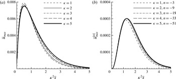
The collapse of these scaled streamwise disturbance velocities onto one profile in the limit of large
 ${\it\kappa}$
and large
 $N$
is confirmed in figure 11. Figure 11(a) shows the collapse of
 $\overline{u}_{max}$
for increasing
 ${\it\kappa}$
. In this time-dependent case, the spacing between coupled modes depends on
 $N$
, and therefore the non-zero coupled modes spread out through the Fourier mode spectrum as
 ${\it\kappa}$
increases, as a consequence of (4.11). This spreading of non-zero modes is illustrated in figure 11(b). A collapse of the profiles is observed, illustrating the robustness of the large-
 ${\it\kappa}$
scaling.
The streamwise evolution of (a)
 $\overline{u}_{max}$
and (b)
 $\overline{u}_{max}^{[n]}$
for the mode
 $2{\it\kappa}^{2}N$
terms removed from the forced mode in the Fourier series.

5. Summary and outlook
The evolution of laminar streaks above a flat plate that oscillates in the spanwise direction has been investigated. Streaks within laminar boundary layers have been observed to be precursors to turbulent transition (Matsubara & Alfredsson Reference Matsubara and Alfredsson2001), and therefore techniques (in this case spanwise plate oscillations) that control their growth have the potential to reduce drag and increase the efficiency of aerofoils and turbomachinery. Variations in streak growth due to different wall oscillation amplitudes, frequencies and free-stream gust properties have been investigated. Reductions in total streak energy have been observed across a wide parameter range.
For the base flow above a spanwise oscillating plate, as a result of the independence principle of Jones (Reference Jones1947), the streamwise and wall-normal momentum equations decouple from the spanwise momentum equation. The streamwise and wall-normal base-flow profiles therefore match the Blasius solution for the flow above a stationary plate, while the spanwise base flow satisfies a generalized streamwise-dependent Stokes layer equation. The streamwise dependence is due to the non-parallel flow effects. The contribution from these terms was neglected in an earlier analysis of this problem (Hack & Zaki Reference Hack and Zaki2012). It has herein been shown that the inclusion of these terms has a crucial effect upon both the base flow and the perturbation flow. These non-parallel terms have the greatest effect for small to moderate streamwise distances, where the laminar streak growth predominates. A WKBJ analysis shows that the GSL tends to the CSL in the limit of either large streamwise distances or high-frequency oscillations. If a classical Stokes spanwise base flow is used instead of the generalized Stokes spanwise base flow, significant deviations manifest themselves in the resulting laminar streak profiles. Large variations in the modal streamwise velocities are observed even when the total r.m.s. streamwise velocity and the total streak energy are comparable. Therefore the use of the CSL as spanwise base flow is inappropriate and can produce both under- and overestimates of the streak energy, depending on the nature of the free-stream forcing and the Strouhal number.
Evolution equations have been determined and solved for the disturbance flow above a spanwise oscillating plate. Even when nonlinear terms are neglected in the regime of initial streak growth, a linear coupling exists between the velocity components, indicating that the secondary flow structures do not obey the independence principle of Jones (Reference Jones1947).
When interacting with the spanwise base flow, the laminar streaks are affected by a range of parameters, including the spanwise plate oscillation amplitude, the Strouhal number (which is a measure of the frequency ratio between the free-stream disturbance and the plate oscillations) and the properties of the free-stream gusts. The latter are particularly important in the current formulation, as the free-stream gust directly forces the laminar streak growth via a mechanism that follows a generalization of the matched asymptotic analysis of Leib et al. (Reference Leib, Wundrow and Goldstein1999) for the flow above a stationary plate. This link between the free-stream gust properties and the laminar streak evolution enables a direct analysis of the former upon the latter. It represents a distinctive feature of the current methodology when compared to approaches based on optimal growth theory, where forcing by the free stream is entirely absent (Andersson et al. Reference Andersson, Berggren and Henningson1999; Luchini Reference Luchini2000) and on models that incorrectly rely on the continuous spectrum of the Orr–Sommerfeld equation to generate free-stream forcing (Hack & Zaki Reference Hack and Zaki2012), as shown by Dong & Wu (Reference Dong and Wu2013a ,Reference Dong and Wu b ).
Reductions in total streak energy in excess of 80 % are found for streaks with
 ${\it\kappa}=1$
,
 $W_{m}>18$
and
 $N=1$
. Two sets of scaled large-
 ${\it\kappa}$
solutions have been obtained, which extend the earlier analysis of LWG99 for the stationary-wall case.
The spanwise wall oscillation technique joins a growing collection of possible methods for delaying laminar–turbulent transition, which also includes boundary-layer suction, boundary-layer cooling and steady spanwise wall forcing. Further experimental investigation is required to confirm the effectiveness of this particular approach. The inherent three-dimensionality of the boundary-layer structures described herein makes the experimental investigation of these phenomena challenging. A single three-dimensional vortical gust can be created using a thin vibrating wire located in the free stream, parallel to the flat plate, and placed at an angle with respect to the oncoming base flow (Wu Reference Wu2001). Further investigation is also required to generalize the existing stability analyses for the CSL (see e.g. Hall Reference Hall1978; Luo & Wu Reference Luo and Wu2010) to the GSL case.
Acknowledgements
The work was partially supported by EPSRC First Grant EP/I033173/1. This research used computing resources at the University of Aberdeen and the University of Sheffield. We would like to thank C. Alvarenga, E. Marensi and E. Zincone for reading a preliminary version of the manuscript and for providing insightful comments.
Appendix A. Initial conditions for spanwise base-flow momentum equation
This appendix presents the initial conditions for the spanwise base-flow momentum equation (2.11) for
 $\overline{x}\ll 1$
. In this limit, a power series solution for
 $W$
is sought with the form
 $$\begin{eqnarray}W(\overline{x},{\it\eta})\sim W_{0}({\it\eta})+2\overline{x}W_{1}({\it\eta})+O(\overline{x}^{2}).\end{eqnarray}$$
Note that, unlike the small-
 $\overline{x}$
series solution of the disturbance equations calculated by LWG99, equation (2.11) does not involve terms of the order of
 $\overline{x}^{1/2}$
. Terms of this magnitude are therefore not required in expansion (A 1). For
 $\overline{x}\ll 1$
, matching coefficients at
 $O(1)$
leads to
 $$\begin{eqnarray}W_{0}^{\prime \prime }+FW_{0}^{\prime }=0,\end{eqnarray}$$
subject to
 $W_{0}(0)=W_{m}$
and
 $W_{0}\rightarrow 0$
as
 ${\it\eta}\rightarrow \infty$
. From the Blasius equation (2.7), it follows that
 $$\begin{eqnarray}W_{0}({\it\eta})=W_{m}(1-F^{\prime })=\frac{k_{z}}{k_{x}}\mathscr{W}_{m}(1-F^{\prime }).\end{eqnarray}$$
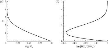
The profile of
 $W_{0}({\it\eta})/W_{m}=1-F^{\prime }$
, shown in figure 12(a), proves that the initial spanwise boundary-layer thickness equals the streamwise boundary-layer thickness, as a result of their common dependence upon
 $F^{\prime }$
. Matching coefficients at
 $O(\overline{x})$
gives
 $$\begin{eqnarray}W_{1}^{\prime \prime }+FW_{1}^{\prime }=\text{i}\overline{{\it\omega}}W_{0}=\text{i}\overline{{\it\omega}}W_{m}(1-F^{\prime })=\frac{\text{i}\overline{{\it\omega}}k_{z}}{k_{x}}\mathscr{W}_{m}(1-F^{\prime }),\end{eqnarray}$$
subject to the boundary conditions
 $W_{1}(0)=0$
and
 $W_{1}\rightarrow 0$
as
 ${\it\eta}\rightarrow \infty$
. The solution to (A 4) is
 $$\begin{eqnarray}W_{1}({\it\eta})=\text{i}\overline{{\it\omega}}W_{m}\left(\int _{0}^{{\it\eta}}F^{\prime \prime }\int _{0}^{\tilde{{\it\eta}}}\frac{1-F^{\prime }}{F^{\prime \prime }}\,\text{d}\breve{{\it\eta}}\text{d}\tilde{{\it\eta}}-F^{\prime }{\it\Delta}\right)\!,\end{eqnarray}$$
where
 $$\begin{eqnarray}{\it\Delta}=\int _{0}^{\infty }F^{\prime \prime }\int _{0}^{\tilde{{\it\eta}}}\frac{1-F^{\prime }}{F^{\prime \prime }}\,\text{d}\breve{{\it\eta}}\,\text{d}\tilde{{\it\eta}}=1.713.\end{eqnarray}$$
From (A 3) and (A 4),
 $\text{Re}\left[W_{1}({\it\eta})\right]=0$
. The profile of
 $\text{Im}\left[W_{1}({\it\eta})\right]/(\overline{{\it\omega}}\,W_{m})$
is shown in figure 12(b).
Profiles of (a) the leading-order base flow
 $W_{0}({\it\eta})/W_{m}$
, and (b) the imaginary part of
 $W_{1}({\it\eta})/(\overline{{\it\omega}}W_{m})$
.

Appendix B. Initial and free-stream boundary conditions for the boundary region equations
In this appendix, the initial and free-stream boundary conditions for the forced and unforced modes are described. The spanwise base flow
 $W\rightarrow 0$
as
 ${\it\eta}\rightarrow \infty$
, and consequently, for the forced mode, the large-
 ${\it\eta}$
LUBR equations are identical to those given on p. 181 of LWG99, as the unforced modes all decay in the far field. Therefore, given the additional factor
 $Q$
in (2.13), the solution of (2.17) that matches with the free-stream gust satisfies
 $$\begin{eqnarray}\overline{u}^{[n]}\rightarrow 0,\end{eqnarray}$$
 $$\begin{eqnarray}\displaystyle & & \displaystyle \displaystyle \left[\frac{\partial }{\partial {\it\eta}}+\left|{\it\kappa}_{z}\right|(2\overline{x})^{1/2}\right]\{\overline{v}^{[n]},\overline{w}^{[n]},\overline{p}^{[n]}\}\nonumber\\ \displaystyle & & \displaystyle \quad \rightarrow \{-1,{\it\kappa}_{y}(2\overline{x})^{1/2},0\}{\it\delta}_{jn}Q\,\text{e}^{-\text{i}\,j\overline{x}+\text{i}{\it\kappa}_{y}(2\overline{x})^{1/2}\overline{{\it\eta}}-({\it\kappa}_{y}^{2}+{\it\kappa}_{z}^{2})\overline{x}},\end{eqnarray}$$
 ${\it\eta}\rightarrow \infty$
, where
 $\overline{{\it\eta}}={\it\eta}-{\it\beta}$
, with
 ${\it\beta}$
defined immediately after (2.7), and
 ${\it\kappa}_{y}=k_{y}/\sqrt{k_{x}\mathit{ Re }_{{\it\lambda}}}$
. The position
 $j$
of the forced mode in the Fourier series takes the value
 $j=-1$
for integer-valued Strouhal numbers. The Kronecker delta,
 $$\begin{eqnarray}{\it\delta}_{jn}=\left\{\begin{array}{@{}ll@{}}0,\quad & j\neq n,\\ 1,\quad & j=n,\end{array}\right.\end{eqnarray}$$
is used to indicate that the only non-zero contribution is from the forced
 $n=j$
mode. On the plate,
 $\overline{u}^{[n]}=\overline{v}^{[n]}=\overline{w}^{[n]}=0$
in order to satisfy no-slip and no-penetration conditions.
The initial conditions for
 ${\it\eta}=O(1)$
are obtained via a small-
 $\overline{x}$
power series of the form
 $$\begin{eqnarray}\{\overline{u}^{[n]},\overline{v}^{[n]},\overline{w}^{[n]},\overline{p}^{[n]}\}=\mathop{\sum }_{i=0}^{\infty }(2\overline{x})^{i/2}\left\{2\overline{x}\overline{U}_{i}^{[n]}({\it\eta}),\overline{V}_{i}^{[n]}({\it\eta}),-\text{i}\overline{W}_{i}^{[n]}({\it\eta}),\frac{\overline{P}_{i}^{[n]}({\it\eta})}{(2\overline{x})^{1/2}}\right\}\!,\end{eqnarray}$$
using the method outlined on p. 182 of LWG99. Upon asymptotic matching with the free-stream behaviour, the initial conditions are
 $$\begin{eqnarray}\overline{u}^{[n]}\sim {\it\delta}_{jn}Q\{2\overline{x}\,\overline{U}_{0}^{[n]}+(2\overline{x})^{3/2}\overline{U}_{1}^{[n]}\},\end{eqnarray}$$
 $$\begin{eqnarray}\displaystyle & & \displaystyle \overline{v}^{[n]}\sim {\it\delta}_{jn}Q\left\{\overline{V}_{0}^{[n]}+(2\overline{x})^{1/2}\overline{V}_{1}^{[n]}\vphantom{\left[-\frac{\text{i}}{2}({\it\kappa}_{y}+\text{i}\left|{\it\kappa}_{z}\right|)(1+\bar{{\it\eta}}^{2})+\frac{\left|{\it\kappa}_{z}\right|g_{1}^{[n]}}{2}+\frac{3{\it\beta}\left|{\it\kappa}_{z}\right|\bar{{\it\eta}}}{4}\right]}\right.\nonumber\\ \displaystyle & & \displaystyle \qquad \;\;+\,\frac{\text{i}\text{e}^{-\text{i}\,j\overline{x}}}{({\it\kappa}_{y}-\text{i}\left|{\it\kappa}_{z}\right|)(2\overline{x})^{1/2}}[\text{e}^{\text{i}{\it\kappa}_{y}(2\overline{x})^{1/2}\bar{{\it\eta}}-({\it\kappa}_{y}^{2}+{\it\kappa}_{z}^{2})\overline{x}}-\text{e}^{-\left|{\it\kappa}_{z}\right|(2\overline{x})^{1/2}\bar{{\it\eta}}}]\nonumber\\ \displaystyle & & \displaystyle \qquad \;\;-\,\text{e}^{-\text{i}\,j\overline{x}-\left|{\it\kappa}_{z}\right|(2\overline{x})^{1/2}\bar{{\it\eta}}}\left[\frac{3{\it\beta}}{4}-\frac{g_{1}^{[n]}\left|{\it\kappa}_{z}\right|}{2}(2\overline{x})^{1/2}\right]+\bar{{\it\eta}}+\frac{3{\it\beta}}{4}\nonumber\\ \displaystyle & & \displaystyle \qquad \;\;-\,\left.(2\overline{x})^{1/2}\left[-\frac{\text{i}}{2}({\it\kappa}_{y}+\text{i}\left|{\it\kappa}_{z}\right|)(1+\bar{{\it\eta}}^{2})+\frac{\left|{\it\kappa}_{z}\right|g_{1}^{[n]}}{2}+\frac{3{\it\beta}\left|{\it\kappa}_{z}\right|\bar{{\it\eta}}}{4}\right]\right\},\end{eqnarray}$$
 $$\begin{eqnarray}\displaystyle & & \displaystyle \overline{w}^{[n]}\sim -{\it\delta}_{jn}Q\left\{\vphantom{\left[\text{i}\left({\it\kappa}_{y}+\text{i}\left|{\it\kappa}_{z}\right|\right)\bar{{\it\eta}}-\frac{3{\it\beta}\left|{\it\kappa}_{z}\right|}{4}\right]}\overline{W}_{0}^{[n]}({\it\eta})+(2\overline{x})^{1/2}\overline{W}_{1}^{[n]}({\it\eta})\vphantom{\left[\text{i}({\it\kappa}_{y}+\text{i}\left|{\it\kappa}_{z}\right|)\bar{{\it\eta}}-\frac{3{\it\beta}\left|{\it\kappa}_{z}\right|}{4}\right]}\right.\nonumber\\ \displaystyle & & \displaystyle \qquad \;\;+\,\frac{\text{e}^{-\text{i}\,j\overline{x}}}{({\it\kappa}_{y}-\text{i}\left|{\it\kappa}_{z}\right|)}[{\it\kappa}_{y}\text{e}^{\text{i}{\it\kappa}_{y}(2\overline{x})^{1/2}\bar{{\it\eta}}-({\it\kappa}_{y}^{2}+{\it\kappa}_{z}^{2})\overline{x}}-\text{i}\left|{\it\kappa}_{z}\right|\text{e}^{-\left|{\it\kappa}_{z}\right|(2\overline{x})^{1/2}\bar{{\it\eta}}}]\nonumber\\ \displaystyle & & \displaystyle \qquad \;\;-\,\frac{3{\it\beta}\left|{\it\kappa}_{z}\right|}{4}(2\overline{x})^{1/2}\text{e}^{-\text{i}\,j\overline{x}-\left|{\it\kappa}_{z}\right|(2\overline{x})^{1/2}\bar{{\it\eta}}}\nonumber\\ \displaystyle & & \displaystyle \left.\qquad \;\;-\,1-(2\overline{x})^{1/2}\left[\text{i}({\it\kappa}_{y}+\text{i}\left|{\it\kappa}_{z}\right|)\bar{{\it\eta}}-\frac{3{\it\beta}\left|{\it\kappa}_{z}\right|}{4}\right]\right\},\end{eqnarray}$$
 $$\begin{eqnarray}\displaystyle & & \displaystyle \overline{p}^{[n]}\sim {\it\delta}_{jn}Q\left\{P_{1}^{[n]}({\it\eta})+\left[g_{1}^{[n]}-\frac{3{\it\beta}}{4\left|{\it\kappa}_{z}\right|(2\overline{x})^{1/2}}\right]\text{e}^{-\left|{\it\kappa}_{z}\right|(2\overline{x})^{1/2}\overline{{\it\eta}}}-g_{1}^{[n]}-\frac{3{\it\beta}\overline{{\it\eta}}}{4}\right\}.\end{eqnarray}$$
 $$\begin{eqnarray}g_{1}^{[n]}=\frac{2c_{1}^{[n]}}{\left|{\it\kappa}_{z}\right|}+\frac{3{\it\beta}^{2}}{2}+\text{i}\left(\frac{{\it\kappa}_{y}}{\left|{\it\kappa}_{z}\right|}+\text{i}\right)(1+{\it\beta}^{2}),\end{eqnarray}$$
matching the definition given by (B 15) of LWG99 for a single uncoupled forced mode, while
 $c_{1}^{[n]}$
is a constant found through the numerical solution.
In the power series, inter-mode coupling does not commence until the third-order terms in the power series are reached. Therefore, in the absence of forcing, the first and second terms of the small-
 $\overline{x}$
power series are all zero, with the exception of the forced
 $n=m$
mode. The forced-mode terms satisfy the ordinary differential equations (B 1)–(B 8) of LWG99, which have the form
 $$\begin{eqnarray}\displaystyle & 2\overline{U}_{0}^{[j]}-{\it\eta}{\overline{U}_{0}^{[j]}}^{\prime }+{\overline{V}_{0}^{[j]}}^{\prime }+\overline{W}_{0}^{[j]}=0, & \displaystyle\end{eqnarray}$$
 $$\begin{eqnarray}\displaystyle & {\overline{U}_{0}^{[j]}}^{\prime \prime }+F{\overline{U}_{0}^{[j]}}^{\prime }+({\it\eta}F^{\prime \prime }-2F^{\prime })\overline{U}_{0}^{[j]}-F^{\prime \prime }\overline{V}_{0}^{[j]}=0, & \displaystyle\end{eqnarray}$$
 $$\begin{eqnarray}\displaystyle & {\overline{P}_{0}^{[j]}}^{\prime }=0, & \displaystyle\end{eqnarray}$$
 $$\begin{eqnarray}\displaystyle & {\overline{W}_{0}^{[j]}}^{\prime \prime }+F{\overline{W}_{0}^{[j]}}^{\prime }=0 & \displaystyle\end{eqnarray}$$
 $$\begin{eqnarray}\displaystyle & 3\overline{U}_{1}^{[j]}-{\it\eta}{\overline{U}_{1}^{[j]}}^{\prime }+{\overline{V}_{1}^{[j]}}^{\prime }+\overline{W}_{1}^{[j]}=0, & \displaystyle\end{eqnarray}$$
 $$\begin{eqnarray}\displaystyle & {\overline{U}_{1}^{[j]}}^{\prime \prime }+F{\overline{U}_{1}^{[j]}}^{\prime }+({\it\eta}F^{\prime \prime }-3F^{\prime })\overline{U}_{1}^{[j]}-F^{\prime \prime }\overline{V}_{1}^{[j]}=0, & \displaystyle\end{eqnarray}$$
 $$\begin{eqnarray}\displaystyle & {\overline{V}_{0}^{[j]}}^{\prime \prime }+F{\overline{V}_{0}^{[j]}}^{\prime }-({\it\eta}F^{\prime })^{\prime }\overline{V}_{0}^{[j]}+[{\it\eta}({\it\eta}F^{\prime })^{\prime }-F]\overline{U}_{0}^{[j]}={\overline{P}_{1}^{[j]}}^{\prime }, & \displaystyle\end{eqnarray}$$
 $$\begin{eqnarray}\displaystyle & {\overline{W}_{1}^{[j]}}^{\prime \prime }+F{\overline{W}_{1}^{[j]}}^{\prime }-F^{\prime }\overline{W}_{1}^{[j]}=-{\it\kappa}_{z}^{2}\overline{P}_{0}^{[j]}. & \displaystyle\end{eqnarray}$$
Note that inter-mode coupling of the first two terms of the power series of the leading-order velocity components and pressure does not exist. If additional terms of the power series were included, or if the higher-order components
 $\{\overline{u}^{(0)},\overline{v}^{(0)},\overline{w}^{(0)},\overline{p}^{(0)}\}$
of Ricco (Reference Ricco2009) were considered, inter-mode coupling would occur.
Appendix C. Numerical procedures
This appendix outlines the numerical procedure used to solve the LUBR equations (2.17), given the initial and boundary conditions in appendix B. To enable a numerical solution, the doubly infinite Fourier series are truncated so that only modes with indices in the range
 $-N_{f}<n<N_{f}$
are included within the calculation, where
 $N_{f}$
is a positive integer. As one moves away from the forced
 $n=-1$
mode in the Fourier series, the energy contained within each mode decreases, and therefore the remaining modes can be safely neglected for a suitably large value of
 $N_{f}$
.
A second-order central finite-difference scheme is used in the wall-normal direction and a fourth-order backward scheme is used in the streamwise direction to evaluate the Fourier coefficients. Both schemes are implicit. The calculation of coefficients of the velocity components and the pressure for each Fourier mode requires
 $4(2N_{f}+1)$
unknowns to be evaluated at each point. The spanwise plate oscillations and the implicit streamwise discretization method result in linear coupling between the unknowns. The unknown velocity and pressure Fourier coefficients in the linear system are collected together so that:
-
(a) the velocity and pressure coefficients for one Fourier mode and one wall-normal station are grouped first;
-
(b) all the Fourier coefficients at that wall-normal station are then grouped together;
-
(c) starting from the wall, the solution at each wall-normal station is obtained.
The resulting linear system is block tridiagonal, with each (dense) block synthesizing all the velocity and pressure Fourier coefficients at one wall-normal station. The actual value of
 $N_{f}$
is determined by the total energy contained within the Fourier mode, which is dominated by the streamwise disturbance velocity. The value of
 $N_{f}$
for each calculation is chosen so that a further increase in
 $N_{f}$
does not alter the total streak energy
 $E$
by more than 2 %.