2.1 Governing equations

Let us consider the nonlinear interactions of two progressive gravity waves and one hydroacoustic wave in water of uniform depth. A Cartesian coordinate system is adopted with the $x$ -axis and the $y$ -axis located on the mean water plane and the $z$ -axis pointing vertically upwards. Longuet-Higgins (Reference Longuet-Higgins1950) derived the water wave equations together with their boundary conditions in a heavy compressible fluid, in the absence of viscosity and surface tension. The governing equation for the velocity potential has linear, quadratic and cubic terms. Kadri & Stiassnie (Reference Kadri and Stiassnie2013) used the same governing equation as Longuet-Higgins, without the cubic term. Here we use the same equation as Longuet-Higgins without the nonlinear terms. The justification is given in the paper by Longuet-Higgins (Reference Longuet-Higgins1950) itself. Indeed, Longuet-Higgins solved for the velocity potential by using a method of successive approximations. At second order, the velocity potential given by his equation (159) has five types of terms. Longuet-Higgins writes below his equation (169) that the first two terms in equation (159) are negligible compared with the fourth, and then writes a simplified expression for the second-order velocity potential (see his equation (172)). We checked that this is equivalent to neglecting the quadratic terms in the governing equation. Therefore, in our paper, we use the governing equation

(2.1) $$\begin{eqnarray}\displaystyle \frac{\unicode[STIX]{x2202}^{2}\unicode[STIX]{x1D711}}{\unicode[STIX]{x2202}t^{2}}-c^{2}\unicode[STIX]{x1D6FB}^{2}\unicode[STIX]{x1D711}+g\frac{\unicode[STIX]{x2202}\unicode[STIX]{x1D711}}{\unicode[STIX]{x2202}z}=0,\quad -h\leqslant z\leqslant \unicode[STIX]{x1D702}(x,y,t),\;(x,y)\in \mathbb{R}^{2}, & & \displaystyle\end{eqnarray}$$

subject to the boundary conditions:

(2.2) $$\begin{eqnarray}\displaystyle & \displaystyle \frac{\unicode[STIX]{x2202}^{2}\unicode[STIX]{x1D711}}{\unicode[STIX]{x2202}t^{2}}+g\frac{\unicode[STIX]{x2202}\unicode[STIX]{x1D711}}{\unicode[STIX]{x2202}z}+\frac{\unicode[STIX]{x2202}|\unicode[STIX]{x1D6FB}\unicode[STIX]{x1D711}|^{2}}{\unicode[STIX]{x2202}t}+\unicode[STIX]{x1D6FB}\unicode[STIX]{x1D711}\boldsymbol{\cdot }\unicode[STIX]{x1D735}\left(\frac{1}{2}|\unicode[STIX]{x1D6FB}\unicode[STIX]{x1D711}|^{2}\right)=0,\quad \text{on}~z=\unicode[STIX]{x1D702}(x,y,t), & \displaystyle\end{eqnarray}$$

(2.3) $$\begin{eqnarray}\displaystyle & \displaystyle g\unicode[STIX]{x1D702}+\frac{\unicode[STIX]{x2202}\unicode[STIX]{x1D711}}{\unicode[STIX]{x2202}t}+\frac{1}{2}|\unicode[STIX]{x1D735}\unicode[STIX]{x1D711}|^{2}=0,\quad \text{on}~z=\unicode[STIX]{x1D702}(x,y,t), & \displaystyle\end{eqnarray}$$

(2.4) $$\begin{eqnarray}\displaystyle & \displaystyle \lim _{z\rightarrow -h}\frac{\unicode[STIX]{x2202}\unicode[STIX]{x1D711}}{\unicode[STIX]{x2202}z}=0, & \displaystyle\end{eqnarray}$$

where

(2.5) $$\begin{eqnarray}\displaystyle \unicode[STIX]{x1D735}=\boldsymbol{i}\frac{\unicode[STIX]{x2202}}{\unicode[STIX]{x2202}x}+\boldsymbol{j}\frac{\unicode[STIX]{x2202}}{\unicode[STIX]{x2202}y}+\boldsymbol{k}\frac{\unicode[STIX]{x2202}}{\unicode[STIX]{x2202}z} & & \displaystyle\end{eqnarray}$$

is a linear operator with $\boldsymbol{i}$ , $\boldsymbol{j}$ , $\boldsymbol{k}$ denoting the unit vector in the $x$ , $y$ , $z$ direction, $\unicode[STIX]{x1D711}$ is the velocity potential, $\unicode[STIX]{x1D702}$ is the wave elevation, $t$ denotes the time, $h$ is the water depth, $c$ is the speed of sound in water, $g$ is the acceleration due to gravity, respectively. Note that the governing equation (2.1) was also used by Kadri & Stiassnie (Reference Kadri and Stiassnie2013). The pressure field of the water can be obtained by Bernoulli’s equation

(2.6) $$\begin{eqnarray}\displaystyle p & = & \displaystyle p_{a}-\unicode[STIX]{x1D70C}gz-\unicode[STIX]{x1D70C}\left(\frac{\unicode[STIX]{x2202}\unicode[STIX]{x1D711}}{\unicode[STIX]{x2202}t}+\frac{1}{2}\frac{\unicode[STIX]{x2202}\unicode[STIX]{x1D711}^{2}}{\unicode[STIX]{x2202}x}+\frac{1}{2}\frac{\unicode[STIX]{x2202}\unicode[STIX]{x1D711}^{2}}{\unicode[STIX]{x2202}y}+\frac{1}{2}\frac{\unicode[STIX]{x2202}\unicode[STIX]{x1D711}^{2}}{\unicode[STIX]{x2202}z}\right)\nonumber\\ \displaystyle & = & \displaystyle p_{a}-\unicode[STIX]{x1D70C}gz+p_{d},\quad -h\leqslant z\leqslant \unicode[STIX]{x1D702}(x,y,t),~(x,y)\in \mathbb{R}^{2},\end{eqnarray}$$

where $p_{a}-\unicode[STIX]{x1D70C}gz$ is the hydrostatic pressure and $p_{d}$ is the dynamic pressure, $\unicode[STIX]{x1D70C}=1025~\text{kg}~\text{m}^{-3}$ .

The linear solutions of the governing equations (2.1)–(2.4) given by Dalrymple & Rogers (Reference Dalrymple and Rogers2006) read

(2.7) $$\begin{eqnarray}\displaystyle \unicode[STIX]{x1D711}=\frac{g\text{i}\tilde{A}}{2\unicode[STIX]{x1D714}}\frac{\unicode[STIX]{x1D706}\cosh [\unicode[STIX]{x1D706}(h+z)]-\unicode[STIX]{x1D6FE}\sinh [\unicode[STIX]{x1D706}(h+z)]}{\unicode[STIX]{x1D706}\cosh (\unicode[STIX]{x1D706}h)-\unicode[STIX]{x1D6FE}\sinh (\unicode[STIX]{x1D706}h)}\text{e}^{\unicode[STIX]{x1D6FE}z}\text{e}^{\text{i}(\boldsymbol{k}\boldsymbol{\cdot }\boldsymbol{r}-\unicode[STIX]{x1D714}t)}, & & \displaystyle\end{eqnarray}$$

where $\unicode[STIX]{x1D6FE}=g/2c^{2}$ , $k^{2}=\unicode[STIX]{x1D706}^{2}+\unicode[STIX]{x1D714}^{2}/c^{2}-\unicode[STIX]{x1D6FE}^{2}$ and the dispersion relation is given by

(2.8) $$\begin{eqnarray}\displaystyle \unicode[STIX]{x1D714}^{2}=g(\unicode[STIX]{x1D706}^{2}-\unicode[STIX]{x1D6FE}^{2})/[\unicode[STIX]{x1D706}\coth (\unicode[STIX]{x1D706}h)-\unicode[STIX]{x1D6FE}], & & \displaystyle\end{eqnarray}$$

where $\tilde{A}$ denotes the wave amplitude, $\boldsymbol{k}$ is the wavenumber, $k=|\boldsymbol{k}|$ , $\unicode[STIX]{x1D714}$ is the wave frequency and $\boldsymbol{r}=x\boldsymbol{i}+y\boldsymbol{j}$ .

Let $\unicode[STIX]{x1D70E}_{i}$ denote the actual wave frequency of two primary gravity waves. Due to the weakly nonlinearity on the free surface of the water, the actual wave frequency $\unicode[STIX]{x1D70E}_{i}$ is slightly different from the linear frequency $\unicode[STIX]{x1D714}_{i}$ . Write

(2.9) $$\begin{eqnarray}\displaystyle \unicode[STIX]{x1D716}_{i}=\frac{\unicode[STIX]{x1D70E}_{i}}{\unicode[STIX]{x1D714}_{i}},\quad i=1,2, & & \displaystyle\end{eqnarray}$$

where the value of $\unicode[STIX]{x1D716}_{i}$ is slightly different from 1. Then, we define the variables

(2.10) $$\begin{eqnarray}\displaystyle \unicode[STIX]{x1D709}_{i}=\boldsymbol{k}_{i}\boldsymbol{\cdot }\boldsymbol{r}-\unicode[STIX]{x1D70E}_{i}t,\quad i=1,2. & & \displaystyle\end{eqnarray}$$

For steady-state wave systems, all wave amplitudes $a_{i}$ , wavenumbers $\boldsymbol{k}_{i}$ and actual wave frequencies $\unicode[STIX]{x1D70E}_{i}$ , where $i=1,2$ , are time independent. Using the new variables $\unicode[STIX]{x1D709}_{i}$ , the original initial/boundary-value problem governed by (2.1)–(2.4) can be transformed into a boundary-value one. In the new coordinate system ( $\unicode[STIX]{x1D709}_{1}$ , $\unicode[STIX]{x1D709}_{2}$ , $z$ ), the governing equation (2.1) becomes

(2.11) $$\begin{eqnarray}\displaystyle & & \displaystyle \mathop{\sum }_{i=1}^{2}\mathop{\sum }_{j=1}^{2}\unicode[STIX]{x1D70E}_{i}\unicode[STIX]{x1D70E}_{j}\frac{\unicode[STIX]{x2202}^{2}\unicode[STIX]{x1D711}}{\unicode[STIX]{x2202}\unicode[STIX]{x1D709}_{i}\unicode[STIX]{x1D709}_{j}}-c^{2}\mathop{\sum }_{i=1}^{2}\mathop{\sum }_{j=1}^{2}\boldsymbol{k}_{i}\boldsymbol{\cdot }\boldsymbol{k}_{j}\frac{\unicode[STIX]{x2202}^{2}\unicode[STIX]{x1D711}}{\unicode[STIX]{x2202}\unicode[STIX]{x1D709}_{i}\unicode[STIX]{x1D709}_{j}}\nonumber\\ \displaystyle & & \displaystyle \qquad -\,c^{2}\frac{\unicode[STIX]{x2202}^{2}\unicode[STIX]{x1D711}}{\unicode[STIX]{x2202}z^{2}}+g\frac{\unicode[STIX]{x2202}\unicode[STIX]{x1D711}}{\unicode[STIX]{x2202}z}=0,\quad -h\leqslant z\leqslant \unicode[STIX]{x1D702}(\unicode[STIX]{x1D709}_{1},\unicode[STIX]{x1D709}_{2}),\end{eqnarray}$$

subject to the two boundary conditions on the unknown free surface $z=\unicode[STIX]{x1D702}(\unicode[STIX]{x1D709}_{1},\unicode[STIX]{x1D709}_{2})$ ,

(2.12) $$\begin{eqnarray}\displaystyle {\mathcal{N}}_{1}[\unicode[STIX]{x1D711},\unicode[STIX]{x1D70E}_{1},\unicode[STIX]{x1D70E}_{2}] & = & \displaystyle \mathop{\sum }_{i=1}^{2}\mathop{\sum }_{j=1}^{2}\unicode[STIX]{x1D70E}_{i}\unicode[STIX]{x1D70E}_{j}\frac{\unicode[STIX]{x2202}^{2}\unicode[STIX]{x1D711}}{\unicode[STIX]{x2202}\unicode[STIX]{x1D709}_{i}\unicode[STIX]{x1D709}_{j}}+g\frac{\unicode[STIX]{x2202}\unicode[STIX]{x1D711}}{\unicode[STIX]{x2202}z}-2\mathop{\sum }_{i=1}^{2}\unicode[STIX]{x1D70E}_{i}\frac{\unicode[STIX]{x2202}f}{\unicode[STIX]{x2202}\unicode[STIX]{x1D709}_{i}}\nonumber\\ \displaystyle & & \displaystyle +\,\mathop{\sum }_{i=1}^{2}\mathop{\sum }_{j=1}^{2}\boldsymbol{k}_{i}\boldsymbol{\cdot }\boldsymbol{k}_{j}\frac{\unicode[STIX]{x2202}\unicode[STIX]{x1D711}}{\unicode[STIX]{x2202}\unicode[STIX]{x1D709}_{i}}\frac{\unicode[STIX]{x2202}f}{\unicode[STIX]{x2202}\unicode[STIX]{x1D709}_{j}}+\frac{\unicode[STIX]{x2202}\unicode[STIX]{x1D711}}{\unicode[STIX]{x2202}z}\frac{\unicode[STIX]{x2202}f}{\unicode[STIX]{x2202}z}=0,\quad \text{on}~z=\unicode[STIX]{x1D702}(\unicode[STIX]{x1D709}_{1},\unicode[STIX]{x1D709}_{2}),\end{eqnarray}$$

(2.13) $$\begin{eqnarray}\displaystyle {\mathcal{N}}_{2}[\unicode[STIX]{x1D711},\unicode[STIX]{x1D702},\unicode[STIX]{x1D70E}_{1},\unicode[STIX]{x1D70E}_{2}]=\unicode[STIX]{x1D702}-\frac{1}{g}\left(\mathop{\sum }_{i=1}^{2}\unicode[STIX]{x1D70E}_{i}\frac{\unicode[STIX]{x2202}\unicode[STIX]{x1D711}}{\unicode[STIX]{x2202}\unicode[STIX]{x1D709}_{i}}-f\right)=0,\quad \text{on}~z=\unicode[STIX]{x1D702}(\unicode[STIX]{x1D709}_{1},\unicode[STIX]{x1D709}_{2}), & & \displaystyle\end{eqnarray}$$

and one impermeable condition at the bottom,

(2.14) $$\begin{eqnarray}\displaystyle \lim _{z\rightarrow -h}\frac{\unicode[STIX]{x2202}\unicode[STIX]{x1D711}}{\unicode[STIX]{x2202}z}=0, & & \displaystyle\end{eqnarray}$$

where

(2.15) $$\begin{eqnarray}\displaystyle f=\frac{1}{2}\left[\mathop{\sum }_{i=1}^{2}\mathop{\sum }_{j=1}^{2}\boldsymbol{k}_{i}\boldsymbol{\cdot }\boldsymbol{k}_{j}\frac{\unicode[STIX]{x2202}\unicode[STIX]{x1D711}}{\unicode[STIX]{x2202}\unicode[STIX]{x1D709}_{i}}\frac{\unicode[STIX]{x2202}\unicode[STIX]{x1D711}}{\unicode[STIX]{x2202}\unicode[STIX]{x1D709}_{j}}+\left(\frac{\unicode[STIX]{x2202}\unicode[STIX]{x1D711}}{\unicode[STIX]{x2202}z}\right)^{2}\right] & & \displaystyle\end{eqnarray}$$

and ${\mathcal{N}}_{1}$ and ${\mathcal{N}}_{2}$ are two nonlinear operators defined above.

For a steady-state wave system, there is no exchange of wave energy between different wave components, i.e. all physical quantities related to the wave systems are constant. Thus, the steady-state wave elevation $\unicode[STIX]{x1D702}(\unicode[STIX]{x1D709}_{1},\unicode[STIX]{x1D709}_{2})$ can be expressed by

(2.16) $$\begin{eqnarray}\displaystyle \unicode[STIX]{x1D702}(\unicode[STIX]{x1D709}_{1},\unicode[STIX]{x1D709}_{2})=\mathop{\sum }_{m_{1}=0}^{+\infty }\mathop{\sum }_{m_{2}=-\infty }^{+\infty }a_{m_{1},m_{2}}\cos (m_{1}\unicode[STIX]{x1D709}_{1}+m_{2}\unicode[STIX]{x1D709}_{2}), & & \displaystyle\end{eqnarray}$$

where $a_{m_{1},m_{2}}$ is a constant to be determined later. Similarly, according to the governing equations (2.11) and the bottom boundary condition (2.14), the velocity potential $\unicode[STIX]{x1D711}(\unicode[STIX]{x1D709}_{1},\unicode[STIX]{x1D709}_{2},z)$ should be in the form

(2.17) $$\begin{eqnarray}\displaystyle \unicode[STIX]{x1D711}(\unicode[STIX]{x1D709}_{1},\unicode[STIX]{x1D709}_{2},z)=\mathop{\sum }_{m_{1}=0}^{+\infty }\mathop{\sum }_{m_{2}=-\infty }^{+\infty }b_{m_{1},m_{2}}\unicode[STIX]{x1D6F9}_{m_{1},m_{2}}(\unicode[STIX]{x1D709}_{1},\unicode[STIX]{x1D709}_{2},z), & & \displaystyle\end{eqnarray}$$

with the definition

(2.18) $$\begin{eqnarray}\displaystyle \unicode[STIX]{x1D6F9}_{m_{1},m_{2}}(\unicode[STIX]{x1D709}_{1},\unicode[STIX]{x1D709}_{2},z) & = & \displaystyle \frac{\unicode[STIX]{x1D706}_{m_{1},m_{2}}\cosh [\unicode[STIX]{x1D706}_{m_{1},m_{2}}(h+z)]-\unicode[STIX]{x1D6FE}\sinh [\unicode[STIX]{x1D706}_{m_{1},m_{2}}(h+z)]}{\unicode[STIX]{x1D706}_{m_{1},m_{2}}\cosh (\unicode[STIX]{x1D706}_{m_{1},m_{2}}h)-\unicode[STIX]{x1D6FE}\sinh (\unicode[STIX]{x1D706}_{m_{1},m_{2}}h)}\nonumber\\ \displaystyle & & \displaystyle \times \,\text{e}^{\unicode[STIX]{x1D6FE}z}\sin (m_{1}\unicode[STIX]{x1D709}_{1}+m_{2}\unicode[STIX]{x1D709}_{2}),\end{eqnarray}$$

where $b_{m_{1},m_{2}}$ is a constant to be determined later. It should be emphasized that (2.17) automatically satisfies the bottom boundary condition (2.14). It also satisfies the governing equation (2.11), provided that $k_{m_{1},m_{2}}^{2}=\unicode[STIX]{x1D706}_{m_{1},m_{2}}^{2}+\unicode[STIX]{x1D70E}_{m_{1},m_{2}}^{2}/c^{2}-\unicode[STIX]{x1D6FE}^{2}$ , where $k_{m_{1},m_{2}}=|m_{1}\boldsymbol{k}_{1}+m_{2}\boldsymbol{k}_{2}|$ , $\unicode[STIX]{x1D70E}_{m_{1},m_{2}}=m_{1}\unicode[STIX]{x1D70E}_{1}+m_{2}\unicode[STIX]{x1D70E}_{2}$ . Because the nonlinearities in the paper of all examples are weak, we choose $\unicode[STIX]{x1D706}_{m_{1},m_{2}}^{2}\approx k_{m_{1},m_{2}}^{2}-\unicode[STIX]{x1D714}_{m_{1},m_{2}}^{2}/c^{2}+\unicode[STIX]{x1D6FE}^{2}$ , where $\unicode[STIX]{x1D714}_{m_{1},m_{2}}=m_{1}\unicode[STIX]{x1D714}_{1}+m_{2}\unicode[STIX]{x1D714}_{2}$ . The corresponding parameter $\unicode[STIX]{x1D706}$ in (2.7) is $\unicode[STIX]{x1D706}_{m_{1},m_{2}}$ . Thus, the unknown coefficients $a_{m_{1},m_{2}}$ and $b_{m_{1},m_{2}}$ are determined by the two fully nonlinear boundary conditions (2.12) and (2.13). Once the velocity potential is obtained, we can directly obtain the pressure field of the water from (2.6). Here, we focus on the dynamic pressure $p_{d}$ in the whole water field. From (2.17), the dynamic pressure $p_{d}$ is in the form as

(2.19) $$\begin{eqnarray}\displaystyle p_{d}(\unicode[STIX]{x1D709}_{1},\unicode[STIX]{x1D709}_{2},z)=\unicode[STIX]{x1D70C}\mathop{\sum }_{m_{1}=0}^{+\infty }\mathop{\sum }_{m_{2}=-\infty }^{+\infty }\left(\unicode[STIX]{x1D714}_{m_{1},m_{2}}^{2}+\frac{1}{2}k_{m_{1},m_{2}}^{2}-\frac{1}{2}\unicode[STIX]{x1D706}_{m_{1},m_{2}}^{2}\right)b_{m_{1},m_{2}}\unicode[STIX]{x1D6F9}_{m_{1},m_{2}}. & & \displaystyle\end{eqnarray}$$

Based on (1.1a–c ), we consider the case $k_{1}=|\boldsymbol{k}_{1}|$ slightly different from $k_{2}=|\boldsymbol{k}_{2}|$ . When $m_{1}\neq m_{2}$ , the value of $(\unicode[STIX]{x1D714}_{m_{1},m_{2}}^{2}/c^{2}-\unicode[STIX]{x1D6FE}^{2})$ is very small (the frequency $\unicode[STIX]{x1D714}_{i}$ of the primary waves considered in this paper is around $1~\text{s}^{-1}$ ) compared to $k_{m_{1},m_{2}}$ , so that $\unicode[STIX]{x1D706}_{m_{1},m_{2}}\approx k_{m_{1},m_{2}}$ , which represents gravity waves in water of uniform depth. When $m_{1}=m_{2}$ , $k_{m_{1},m_{2}}$ is very small. $\unicode[STIX]{x1D706}_{m_{1},m_{2}}$ is an imaginary number, which represents the hydroacoustic wave. Further, when $m_{1}=m_{2}>1$ , the corresponding hydroacoustic wave is generated by two high-order gravity waves. In this paper, we focus on the resulting hydroacoustic wave, when $m_{1}=m_{2}=1$ .

2.2 Solution procedure

In 2011, Liao (Reference Liao2011b ) successfully applied the HAM to obtain the solutions of steady-state resonant gravity waves governed by the fully nonlinear wave equations. Thereafter, Xu et al. (Reference Xu, Lin, Liao and Stiassnie2012), Liu & Liao (Reference Liu and Liao2014), Liao et al. (Reference Liao, Xu and Stiassnie2016) and Liu et al. (Reference Liu, Xu and Liao2018) made further contributions in the study of steady-state resonant gravity waves. Detailed mathematical derivations can be found in these articles. So, for the sake of simplicity, we just give some important formulae here.

Let $q\in [0,1]$ denote an embedding parameter. In the framework of HAM, we first construct a family of solutions $\unicode[STIX]{x1D6F7}(\unicode[STIX]{x1D709}_{1},\unicode[STIX]{x1D709}_{2},z;q)$ , $\unicode[STIX]{x1D701}(\unicode[STIX]{x1D709}_{1},\unicode[STIX]{x1D709}_{2};q)$ , $\unicode[STIX]{x1D6EC}_{1}(q)$ and $\unicode[STIX]{x1D6EC}_{2}(q)$ in $q\in [0,1]$ by means of the so-called zeroth-order deformation equations,

(2.20) $$\begin{eqnarray}\displaystyle & & \displaystyle \mathop{\sum }_{i=1}^{2}\mathop{\sum }_{j=1}^{2}\unicode[STIX]{x1D70E}_{i}\unicode[STIX]{x1D70E}_{j}\frac{\unicode[STIX]{x2202}^{2}\unicode[STIX]{x1D6F7}}{\unicode[STIX]{x2202}\unicode[STIX]{x1D709}_{i}\unicode[STIX]{x1D709}_{j}}-c^{2}\mathop{\sum }_{i=1}^{2}\mathop{\sum }_{j=1}^{2}\boldsymbol{k}_{i}\boldsymbol{\cdot }\boldsymbol{k}_{j}\frac{\unicode[STIX]{x2202}^{2}\unicode[STIX]{x1D6F7}}{\unicode[STIX]{x2202}\unicode[STIX]{x1D709}_{i}\unicode[STIX]{x1D709}_{j}}\nonumber\\ \displaystyle & & \displaystyle \qquad -\,c^{2}\frac{\unicode[STIX]{x2202}^{2}\unicode[STIX]{x1D6F7}}{\unicode[STIX]{x2202}z^{2}}+g\frac{\unicode[STIX]{x2202}\unicode[STIX]{x1D6F7}}{\unicode[STIX]{x2202}z}=0,\quad -h\leqslant z\leqslant \unicode[STIX]{x1D701}(\unicode[STIX]{x1D709}_{1},\unicode[STIX]{x1D709}_{2};q),\end{eqnarray}$$

subject to the two boundary conditions on the unknown wave elevation $z=\unicode[STIX]{x1D702}(\unicode[STIX]{x1D709}_{1},\unicode[STIX]{x1D709}_{2};q)$

(2.21) $$\begin{eqnarray}\displaystyle & \displaystyle (1-q){\mathcal{L}}^{\ast }[\unicode[STIX]{x1D6F7}(\unicode[STIX]{x1D709}_{1},\unicode[STIX]{x1D709}_{2},z;q)-\unicode[STIX]{x1D711}_{0}(\unicode[STIX]{x1D709}_{1},\unicode[STIX]{x1D709}_{2},z)]\!=\!c_{0}q{\mathcal{N}}_{1}[\unicode[STIX]{x1D6F7}(\unicode[STIX]{x1D709}_{1},\unicode[STIX]{x1D709}_{2},z;q),\unicode[STIX]{x1D6EC}_{1}(q),\unicode[STIX]{x1D6EC}_{2}(q)], & \displaystyle\end{eqnarray}$$

(2.22) $$\begin{eqnarray}\displaystyle & \displaystyle (1-q)\unicode[STIX]{x1D701}(\unicode[STIX]{x1D709}_{1},\unicode[STIX]{x1D709}_{2};q)=c_{0}q{\mathcal{N}}_{2}[\unicode[STIX]{x1D6F7}(\unicode[STIX]{x1D709}_{1},\unicode[STIX]{x1D709}_{2},z;q),\unicode[STIX]{x1D701}(\unicode[STIX]{x1D709}_{1},\unicode[STIX]{x1D709}_{2};q),\unicode[STIX]{x1D6EC}_{1}(q),\unicode[STIX]{x1D6EC}_{2}(q)], & \displaystyle\end{eqnarray}$$

and the impermeable condition at the bottom

(2.23) $$\begin{eqnarray}\displaystyle \lim _{z\rightarrow -h}\frac{\unicode[STIX]{x2202}\unicode[STIX]{x1D6F7}}{\unicode[STIX]{x2202}z}=0, & & \displaystyle\end{eqnarray}$$

where ${\mathcal{N}}_{1}$ and ${\mathcal{N}}_{2}$ are the two nonlinear operators defined by (2.12) and (2.13), ${\mathcal{L}}^{\ast }$ is an auxiliary linear operator and $\unicode[STIX]{x1D711}_{0}(\unicode[STIX]{x1D709}_{1},\unicode[STIX]{x1D709}_{2},z)$ is an initial guess of $\unicode[STIX]{x1D711}(\unicode[STIX]{x1D709}_{1},\unicode[STIX]{x1D709}_{2},z)$ , $c_{0}\neq 0$ is the so-called ‘convergence-control parameter’ without physical meaning, respectively. Here, $\unicode[STIX]{x1D6F7}$ , $\unicode[STIX]{x1D701}$ , $\unicode[STIX]{x1D6EC}_{1}$ , $\unicode[STIX]{x1D6EC}_{2}$ correspond to the unknown $\unicode[STIX]{x1D711}$ , $\unicode[STIX]{x1D702}$ , $\unicode[STIX]{x1D70E}_{1}$ , $\unicode[STIX]{x1D70E}_{2}$ , respectively. It should be emphasized that we have great freedom to choose the auxiliary linear operator. Obviously, when $q=0$ ,

(2.24a,b ) $$\begin{eqnarray}\displaystyle \unicode[STIX]{x1D6F7}(\unicode[STIX]{x1D709}_{1},\unicode[STIX]{x1D709}_{2},z;0)=\unicode[STIX]{x1D711}_{0}(\unicode[STIX]{x1D709}_{1},\unicode[STIX]{x1D709}_{2},z),\quad \unicode[STIX]{x1D701}(\unicode[STIX]{x1D709}_{1},\unicode[STIX]{x1D709}_{2};0)=0. & & \displaystyle\end{eqnarray}$$

When $q=1$ , equations (2.20)–(2.23) are equivalent to the original equations (2.11)–(2.14), respectively, therefore we have

(2.25a-d ) $$\begin{eqnarray}\displaystyle \unicode[STIX]{x1D6F7}(\unicode[STIX]{x1D709}_{1},\unicode[STIX]{x1D709}_{2},z;1)=\unicode[STIX]{x1D711}(\unicode[STIX]{x1D709}_{1},\unicode[STIX]{x1D709}_{2},z),\quad \unicode[STIX]{x1D701}(\unicode[STIX]{x1D709}_{1},\unicode[STIX]{x1D709}_{2};1)=\unicode[STIX]{x1D702}(\unicode[STIX]{x1D709}_{1},\unicode[STIX]{x1D709}_{2}),\quad \unicode[STIX]{x1D6EC}_{1}(1)=\unicode[STIX]{x1D70E}_{1},\quad \unicode[STIX]{x1D6EC}_{2}(1)=\unicode[STIX]{x1D70E}_{2}. & & \displaystyle \nonumber\\ \displaystyle & & \displaystyle\end{eqnarray}$$

Thus, as $q$ increases from 0 to 1, $\unicode[STIX]{x1D6F7}(\unicode[STIX]{x1D709}_{1},\unicode[STIX]{x1D709}_{2},z;q)$ deforms continuously from the initial guess $\unicode[STIX]{x1D711}_{0}(\unicode[STIX]{x1D709}_{1},\unicode[STIX]{x1D709}_{2},z)$ to the unknown potential function $\unicode[STIX]{x1D711}(\unicode[STIX]{x1D709}_{1},\unicode[STIX]{x1D709}_{2},z)$ , so does $\unicode[STIX]{x1D701}(\unicode[STIX]{x1D709}_{1},\unicode[STIX]{x1D709}_{2};q)$ from $0$ to the unknown wave profile $\unicode[STIX]{x1D702}(\unicode[STIX]{x1D709}_{1},\unicode[STIX]{x1D709}_{2})$ , $\unicode[STIX]{x1D6EC}_{1}(q),\unicode[STIX]{x1D6EC}_{2}(q)$ from the initial guesses $\unicode[STIX]{x1D70E}_{1,0},\unicode[STIX]{x1D70E}_{2,0}$ to the unknown frequencies $\unicode[STIX]{x1D70E}_{1},\unicode[STIX]{x1D70E}_{2}$ , respectively.

Assuming that the convergence-control parameter $c_{0}$ is properly chosen so that the Maclaurin series of $\unicode[STIX]{x1D6F7}(\unicode[STIX]{x1D709}_{1},\unicode[STIX]{x1D709}_{2},z;q)$ , $\unicode[STIX]{x1D701}(\unicode[STIX]{x1D709}_{1},\unicode[STIX]{x1D709}_{2};q)$ , $\unicode[STIX]{x1D6EC}_{1}(q)$ and $\unicode[STIX]{x1D6EC}_{2}(q)$ with respect to the embedding parameter $q$ , i.e.

(2.26a,b ) $$\begin{eqnarray}\displaystyle \unicode[STIX]{x1D6F7}(\unicode[STIX]{x1D709}_{1},\unicode[STIX]{x1D709}_{2},z;q)=\mathop{\sum }_{m=0}^{+\infty }\unicode[STIX]{x1D711}_{m}(\unicode[STIX]{x1D709}_{1},\unicode[STIX]{x1D709}_{2},z)q^{m},\quad \unicode[STIX]{x1D701}(\unicode[STIX]{x1D709}_{1},\unicode[STIX]{x1D709}_{2};q)=\mathop{\sum }_{m=0}^{+\infty }\unicode[STIX]{x1D702}_{m}(\unicode[STIX]{x1D709}_{1},\unicode[STIX]{x1D709}_{2})q^{m}, & & \displaystyle\end{eqnarray}$$

(2.26c,d ) $$\begin{eqnarray}\displaystyle \unicode[STIX]{x1D6EC}_{1}(q)=\mathop{\sum }_{m=0}^{+\infty }\unicode[STIX]{x1D70E}_{1,m}q^{m},\quad \unicode[STIX]{x1D6EC}_{2}(q)=\mathop{\sum }_{m=0}^{+\infty }\unicode[STIX]{x1D70E}_{2,m}q^{m} & & \displaystyle\end{eqnarray}$$

exist and converge at $q=1$ , we have the so-called homotopy-series solution

(2.27a,b ) $$\begin{eqnarray}\displaystyle \unicode[STIX]{x1D711}(\unicode[STIX]{x1D709}_{1},\unicode[STIX]{x1D709}_{2},z)=\mathop{\sum }_{m=0}^{+\infty }\unicode[STIX]{x1D711}_{m}(\unicode[STIX]{x1D709}_{1},\unicode[STIX]{x1D709}_{2},z),\quad \unicode[STIX]{x1D702}(\unicode[STIX]{x1D709}_{1},\unicode[STIX]{x1D709}_{2})=\mathop{\sum }_{m=0}^{+\infty }\unicode[STIX]{x1D702}_{m}(\unicode[STIX]{x1D709}_{1},\unicode[STIX]{x1D709}_{2}), & & \displaystyle\end{eqnarray}$$

(2.27c,d ) $$\begin{eqnarray}\displaystyle \unicode[STIX]{x1D70E}_{1}=\mathop{\sum }_{m=0}^{+\infty }\unicode[STIX]{x1D70E}_{1,m},\quad \unicode[STIX]{x1D70E}_{2}=\mathop{\sum }_{m=0}^{+\infty }\unicode[STIX]{x1D70E}_{2,m}, & & \displaystyle\end{eqnarray}$$

respectively.

Substituting the Maclaurin series (2.26) into the zeroth-order deformation equations (2.20)–(2.23) and then equating the like powers of $q$ , we obtain the so-called high-order deformation equations

(2.28) $$\begin{eqnarray}\displaystyle & & \displaystyle \mathop{\sum }_{i=1}^{2}\mathop{\sum }_{j=1}^{2}\unicode[STIX]{x1D70E}_{i}\unicode[STIX]{x1D70E}_{j}\frac{\unicode[STIX]{x2202}^{2}\unicode[STIX]{x1D711}_{m}}{\unicode[STIX]{x2202}\unicode[STIX]{x1D709}_{i}\unicode[STIX]{x1D709}_{j}}-c^{2}\mathop{\sum }_{i=1}^{2}\mathop{\sum }_{j=1}^{2}\boldsymbol{k}_{i}\boldsymbol{\cdot }\boldsymbol{k}_{j}\frac{\unicode[STIX]{x2202}^{2}\unicode[STIX]{x1D711}_{m}}{\unicode[STIX]{x2202}\unicode[STIX]{x1D709}_{i}\unicode[STIX]{x1D709}_{j}}\nonumber\\ \displaystyle & & \displaystyle \qquad -\,c^{2}\frac{\unicode[STIX]{x2202}^{2}\unicode[STIX]{x1D711}_{m}}{\unicode[STIX]{x2202}z^{2}}+g\frac{\unicode[STIX]{x2202}\unicode[STIX]{x1D711}_{m}}{\unicode[STIX]{x2202}z}=0,\quad -h\leqslant z\leqslant 0,\end{eqnarray}$$

subject to the linear boundary condition

(2.29) $$\begin{eqnarray}\displaystyle {\mathcal{L}}^{\ast }[\unicode[STIX]{x1D711}_{m}]=c_{0}\unicode[STIX]{x1D6E5}_{m-1}^{\unicode[STIX]{x1D711}}+\unicode[STIX]{x1D712}_{m}S_{m-1}-\bar{S}_{m},\quad \text{on}~z=0, & & \displaystyle\end{eqnarray}$$

and the bottom condition

(2.30) $$\begin{eqnarray}\displaystyle \frac{\unicode[STIX]{x2202}\unicode[STIX]{x1D711}_{m}}{\unicode[STIX]{x2202}z}=0,\quad \text{as}~z\rightarrow -h, & & \displaystyle\end{eqnarray}$$

together with

(2.31) $$\begin{eqnarray}\displaystyle \unicode[STIX]{x1D702}_{m}=c_{0}\unicode[STIX]{x1D6E5}_{m-1}^{\unicode[STIX]{x1D702}}+\unicode[STIX]{x1D712}_{m}\unicode[STIX]{x1D702}_{m-1},\quad \text{on}~z=0, & & \displaystyle\end{eqnarray}$$

where $\unicode[STIX]{x1D712}_{1}=0$ and $\unicode[STIX]{x1D712}_{m}=1$ for $m>1$ . $\bar{S}_{m}$ and $S_{m}$ are dependent upon the chosen auxiliary linear operator and thus will be given later. The definitions of $\unicode[STIX]{x1D6E5}_{m-1}^{\unicode[STIX]{x1D711}}$ and $\unicode[STIX]{x1D6E5}_{m-1}^{\unicode[STIX]{x1D702}}$ are given in the Appendix. Note that all of the $\unicode[STIX]{x1D6E5}_{m-1}^{\unicode[STIX]{x1D711}}$ , $\unicode[STIX]{x1D6E5}_{m-1}^{\unicode[STIX]{x1D702}}$ , $\bar{S}_{m}$ and $S_{m}$ on the right-hand side of (2.29) and (2.31) are determined by the known previous approximations $\unicode[STIX]{x1D702}_{j}$ and $\unicode[STIX]{x1D711}_{j}~(j=0,1,2,\ldots ,m-1)$ , and thus can be regarded as known terms.

2.3 Small denominators of the acoustic–gravity waves

Let ${\mathcal{L}}$ denote a differential operator corresponding to the linear parts of (2.12), i.e.

(2.32) $$\begin{eqnarray}\displaystyle {\mathcal{L}}[\unicode[STIX]{x1D711}]=\unicode[STIX]{x1D714}_{1}^{2}\frac{\unicode[STIX]{x2202}^{2}\unicode[STIX]{x1D711}}{\unicode[STIX]{x2202}\unicode[STIX]{x1D709}_{1}^{2}}+2\unicode[STIX]{x1D714}_{1}\unicode[STIX]{x1D714}_{2}\frac{\unicode[STIX]{x2202}^{2}\unicode[STIX]{x1D711}}{\unicode[STIX]{x2202}\unicode[STIX]{x1D709}_{1}\unicode[STIX]{x2202}\unicode[STIX]{x1D709}_{2}}+\unicode[STIX]{x1D714}_{2}^{2}\frac{\unicode[STIX]{x2202}^{2}\unicode[STIX]{x1D711}}{\unicode[STIX]{x2202}\unicode[STIX]{x1D709}_{2}^{2}}+g\frac{\unicode[STIX]{x2202}\unicode[STIX]{x1D711}}{\unicode[STIX]{x2202}z}, & & \displaystyle\end{eqnarray}$$

which has the property

(2.33) $$\begin{eqnarray}\displaystyle {\mathcal{L}}[\unicode[STIX]{x1D6F9}_{m_{1},m_{2}}(\unicode[STIX]{x1D709}_{1},\unicode[STIX]{x1D709}_{2}),z]=\tilde{\unicode[STIX]{x1D706}}_{m_{1},m_{2}}\unicode[STIX]{x1D6F9}_{m_{1},m_{2}}(\unicode[STIX]{x1D709}_{1},\unicode[STIX]{x1D709}_{2}), & & \displaystyle\end{eqnarray}$$

where

(2.34) $$\begin{eqnarray}\displaystyle \tilde{\unicode[STIX]{x1D706}}_{m_{1},m_{2}}=\frac{g(\unicode[STIX]{x1D706}_{m_{1},m_{2}}^{2}-\unicode[STIX]{x1D6FE}^{2})}{\unicode[STIX]{x1D706}_{m_{1},m_{2}}\coth (\unicode[STIX]{x1D706}_{m_{1},m_{2}}h)-\unicode[STIX]{x1D6FE}}-(m_{1}\unicode[STIX]{x1D714}_{1}+m_{2}\unicode[STIX]{x1D714}_{2})^{2}. & & \displaystyle\end{eqnarray}$$

Therefore, its inverse operator ${\mathcal{L}}^{-1}$ is given by

(2.35) $$\begin{eqnarray}\displaystyle {\mathcal{L}}^{-1}[\unicode[STIX]{x1D6F9}_{m_{1},m_{2}}(\unicode[STIX]{x1D709}_{1},\unicode[STIX]{x1D709}_{2},z)]=\frac{\unicode[STIX]{x1D6F9}_{m_{1},m_{2}}(\unicode[STIX]{x1D709}_{1},\unicode[STIX]{x1D709}_{2},z)}{\tilde{\unicode[STIX]{x1D706}}_{m_{1},m_{2}}}. & & \displaystyle\end{eqnarray}$$

Considering the gravity wave components ( $m_{1}\neq m_{2}$ ), $\tilde{\unicode[STIX]{x1D706}}_{m_{1},m_{2}}\approx g|m_{1}\boldsymbol{k}_{1}+m_{2}\boldsymbol{k}_{2}|-(m_{1}\unicode[STIX]{x1D714}_{1}+m_{2}\unicode[STIX]{x1D714}_{2})^{2}$ . And based on (1.1), we have $k_{1}\approx k_{2}=k$ and $\unicode[STIX]{x1D714}_{1}\approx \unicode[STIX]{x1D714}_{2}=\sqrt{gk}$ . For gravity wave components, when $\tilde{\unicode[STIX]{x1D706}}_{m_{1},m_{2}}\approx 0$ , we have

(2.36) $$\begin{eqnarray}\displaystyle |m_{1}-m_{2}|-(m_{1}+m_{2})^{2}\approx 0. & & \displaystyle\end{eqnarray}$$

The above equation has an infinite number of integer solutions, as shown in table 1, corresponding to an infinite number of small denominators. Thus, it is very difficult to obtain the steady-state acoustic–gravity waves by traditional methods such as perturbation methods. Considering the hydroacoustic wave components ( $m_{1}=m_{2}$ ), when the resonance condition (1.3) is satisfied, one more zero denominator $\tilde{\unicode[STIX]{x1D706}}_{1,1}=0$ must be considered.

2.4 Choice of auxiliary linear operator

There exists an infinite number of small denominators even in the case of non-resonance. In the framework of perturbation techniques, it is rather difficult to handle such an infinite number of small denominators. However, different from perturbation methods, HAM provides us great freedom to choose the auxiliary linear operator, so that we can choose an auxiliary linear operator that is different from (2.32). Such kind of freedom of the HAM allows us to choose an appropriate auxiliary linear operator to avoid an infinite number of small denominators conveniently, as mentioned below.

Table 1.

The values of $(m_{1},m_{2})$ corresponding to $\tilde{\unicode[STIX]{x1D706}}_{m_{1},m_{2}}\approx 0$ .

Using the freedom of the HAM mentioned above, we choose such an auxiliary linear operator

(2.37) $$\begin{eqnarray}\displaystyle {\mathcal{L}}^{\ast }[\unicode[STIX]{x1D711}]=\unicode[STIX]{x1D714}_{1}^{2}\frac{\unicode[STIX]{x2202}^{2}\unicode[STIX]{x1D711}}{\unicode[STIX]{x2202}\unicode[STIX]{x1D709}_{1}^{2}}+2\unicode[STIX]{x1D714}_{1}\unicode[STIX]{x1D714}_{2}\frac{\unicode[STIX]{x2202}^{2}\unicode[STIX]{x1D711}}{\unicode[STIX]{x2202}\unicode[STIX]{x1D709}_{1}\unicode[STIX]{x2202}\unicode[STIX]{x1D709}_{2}}+\unicode[STIX]{x1D714}_{2}^{2}\frac{\unicode[STIX]{x2202}^{2}\unicode[STIX]{x1D711}}{\unicode[STIX]{x2202}\unicode[STIX]{x1D709}_{2}^{2}}+\unicode[STIX]{x1D707}g\frac{\unicode[STIX]{x2202}\unicode[STIX]{x1D711}}{\unicode[STIX]{x2202}z}, & & \displaystyle\end{eqnarray}$$

where

(2.38) $$\begin{eqnarray}\displaystyle \unicode[STIX]{x1D707}=\left\{\begin{array}{@{}ll@{}}1, & m_{1}=1,m_{2}=0;m_{1}=0,m_{2}=1,\\ \unicode[STIX]{x03C0}/3, & \text{else},\end{array}\right. & & \displaystyle\end{eqnarray}$$

which has the property

(2.39) $$\begin{eqnarray}\displaystyle {\mathcal{L}}^{\ast }[\unicode[STIX]{x1D6F9}_{m_{1},m_{2}}(\unicode[STIX]{x1D709}_{1},\unicode[STIX]{x1D709}_{2}),z]=\tilde{\unicode[STIX]{x1D706}}_{m_{1},m_{2}}^{\ast }\unicode[STIX]{x1D6F9}_{m_{1},m_{2}}(\unicode[STIX]{x1D709}_{1},\unicode[STIX]{x1D709}_{2}), & & \displaystyle\end{eqnarray}$$

where

(2.40) $$\begin{eqnarray}\displaystyle \tilde{\unicode[STIX]{x1D706}}_{m_{1},m_{2}}^{\ast }=\frac{\unicode[STIX]{x1D707}g(\unicode[STIX]{x1D706}_{m_{1},m_{2}}^{2}-\unicode[STIX]{x1D6FE}^{2})}{\unicode[STIX]{x1D706}_{m_{1},m_{2}}\coth (\unicode[STIX]{x1D706}_{m_{1},m_{2}}h)-\unicode[STIX]{x1D6FE}}-(m_{1}\unicode[STIX]{x1D714}_{1}+m_{2}\unicode[STIX]{x1D714}_{2})^{2}. & & \displaystyle\end{eqnarray}$$

So its inverse operator ${\mathcal{L}}^{\ast -1}$ reads

(2.41) $$\begin{eqnarray}\displaystyle {\mathcal{L}}^{\ast -1}[\unicode[STIX]{x1D6F9}_{m_{1},m_{2}}(\unicode[STIX]{x1D709}_{1},\unicode[STIX]{x1D709}_{2},z)]=\frac{\unicode[STIX]{x1D6F9}_{m_{1},m_{2}}(\unicode[STIX]{x1D709}_{1},\unicode[STIX]{x1D709}_{2},z)}{\tilde{\unicode[STIX]{x1D706}}_{m_{1},m_{2}}^{\ast }}. & & \displaystyle\end{eqnarray}$$

When considering the gravity wave components ( $m_{1}\neq m_{2}$ ) and $\tilde{\unicode[STIX]{x1D706}}_{m_{1},m_{2}}^{\ast }\approx 0$ , we have

(2.42) $$\begin{eqnarray}\displaystyle \unicode[STIX]{x1D707}|m_{1}-m_{2}|-(m_{1}+m_{2})^{2}\approx 0, & & \displaystyle\end{eqnarray}$$

which does not have an infinite number of integer solutions. When $m_{1}=1,m_{2}=0$ and $m_{1}=0,m_{2}=1$ , the auxiliary linear operators ${\mathcal{L}}^{\ast }$ and ${\mathcal{L}}$ in (2.32) are the same, $\tilde{\unicode[STIX]{x1D706}}_{1,0}^{\ast }=\tilde{\unicode[STIX]{x1D706}}_{0,1}^{\ast }=0$ . For the rest, we choose $\unicode[STIX]{x1D707}=\unicode[STIX]{x03C0}/3$ as an irrational number. When $m_{1}=m_{2}$ , $\unicode[STIX]{x1D707}|m_{1}-m_{2}|=0$ , $-(m_{1}+m_{2})^{2}\not =0$ . When $m_{1}\not =m_{2}$ , $\unicode[STIX]{x1D707}|m_{1}-m_{2}|$ is a non-zero irrational number but $-(m_{1}+m_{2})^{2}$ is a rational number, therefore it holds that $\unicode[STIX]{x1D707}|m_{1}-m_{2}|-(m_{1}+m_{2})^{2}\not =0$ , because the sum of a rational number and a non-zero irrational number is always a non-zero irrational number. In this way, equation (2.42) has only two integer solutions: $m_{1}=1,m_{2}=0$ and $m_{1}=0,m_{2}=1$ . Thus, we have $\tilde{\unicode[STIX]{x1D706}}_{m_{1},m_{2}}^{\ast }=0$ for only two cases even for resonance conditions:

(2.43) $$\begin{eqnarray}\displaystyle \tilde{\unicode[STIX]{x1D706}}_{1,0}^{\ast }=\tilde{\unicode[STIX]{x1D706}}_{0,1}^{\ast }=0. & & \displaystyle\end{eqnarray}$$

Until now, with the proper auxiliary linear operator, an infinite number of small denominators are avoided once and for all automatically. It should be emphasized that we choose two different values of $\unicode[STIX]{x1D707}$ ( $\unicode[STIX]{x03C0}/3$ and $\sqrt{2}$ ) but obtain the same result. So, without loss of generality, we choose $\unicode[STIX]{x1D707}=\unicode[STIX]{x03C0}/3$ in the calculations of this paper.

Based on the auxiliary linear operator (2.37), $\bar{S}_{m}$ and $S_{m}$ in high-order deformation equations are defined by

(2.44) $$\begin{eqnarray}\displaystyle & \displaystyle \bar{S}_{m}=\mathop{\sum }_{n=1}^{m-1}(\unicode[STIX]{x1D714}_{1}^{2}\unicode[STIX]{x1D6FD}_{2,0}^{m-n,n}+2\unicode[STIX]{x1D714}_{1}\unicode[STIX]{x1D714}_{2}\unicode[STIX]{x1D6FD}_{1,1}^{m-n,n}+\unicode[STIX]{x1D714}_{2}^{2}\unicode[STIX]{x1D6FD}_{0,2}^{m-n,n}+\unicode[STIX]{x1D707}g\unicode[STIX]{x1D6FE}_{0,0}^{m-n,n}), & \displaystyle\end{eqnarray}$$

(2.45) $$\begin{eqnarray}\displaystyle & \displaystyle S_{m}=\unicode[STIX]{x1D714}_{1}^{2}\unicode[STIX]{x1D6FD}_{2,0}^{m,0}+2\unicode[STIX]{x1D714}_{1}\unicode[STIX]{x1D714}_{2}\unicode[STIX]{x1D6FD}_{1,1}^{m,0}+\unicode[STIX]{x1D714}_{2}^{2}\unicode[STIX]{x1D6FD}_{0,2}^{m,0}+\unicode[STIX]{x1D707}g\unicode[STIX]{x1D6FE}_{0,0}^{m,0}+\bar{S}_{m}, & \displaystyle\end{eqnarray}$$

where $\unicode[STIX]{x1D6FD}_{i,j}^{n,m}$ and $\unicode[STIX]{x1D6FE}_{i,j}^{n,m}$ are defined by (A 19) and (A 20).

2.5 Choice of the initial guess

In case of non-resonance, using the freedom of the HAM in the choice of the initial guess solution $\unicode[STIX]{x1D711}_{0}$ , we let the initial guess $\unicode[STIX]{x1D711}_{0}$ contain two non-trivial components

(2.46) $$\begin{eqnarray}\displaystyle \unicode[STIX]{x1D711}_{0}=A\frac{g}{\unicode[STIX]{x1D714}}\unicode[STIX]{x1D6F9}_{1,0}+B\frac{g}{\unicode[STIX]{x1D714}}\unicode[STIX]{x1D6F9}_{0,1}, & & \displaystyle\end{eqnarray}$$

where $\unicode[STIX]{x1D714}_{1}=\unicode[STIX]{x1D714}_{2}=\unicode[STIX]{x1D714}$ , $A$ and $B$ are constants, which will be chosen for different cases. The real frequencies $\unicode[STIX]{x1D70E}_{1,0}$ and $\unicode[STIX]{x1D70E}_{2,0}$ are unknown.

In the case of resonating triads, $\tilde{\unicode[STIX]{x1D706}}_{1,1}=0$ corresponding to the resonant hydroacoustic wave component must be considered. Assuming that the resonant hydroacoustic wave occupies a significant energy (compared to the non-resonance case) in the wave system, our strategy is to add the resonant hydroacoustic wave component to the initial guess so that the initial guess is closer to the exact solution, which will make for rapid convergence. With the great freedom in the choice of the initial guess, we let the initial guess $\unicode[STIX]{x1D711}_{0}$ contain two non-trivial components and one resonant component

(2.47) $$\begin{eqnarray}\displaystyle \unicode[STIX]{x1D711}_{0}=A\frac{g}{\unicode[STIX]{x1D714}}\unicode[STIX]{x1D6F9}_{1,0}+B\frac{g}{\unicode[STIX]{x1D714}}\unicode[STIX]{x1D6F9}_{0,1}+C\frac{g}{2\unicode[STIX]{x1D714}}\unicode[STIX]{x1D6F9}_{1,1}, & & \displaystyle\end{eqnarray}$$

where $A$ and $B$ are constants, which will be chosen for different cases. $C$ is related to $A$ and $B$ . It is found that, when $C=\min \{A,B\}$ , convergence can be obtained in all cases in which the steady-state resonant acoustic–gravity waves exist in the present paper.

3.1 Non-resonant waves

For acoustic–gravity waves far from resonance, we take the same case as that considered by Kadri & Stiassnie (Reference Kadri and Stiassnie2013):

(3.1a ) $$\begin{eqnarray}\displaystyle & \displaystyle \boldsymbol{k}_{1}=(0.101937,0)~\text{m}^{-1},\quad \unicode[STIX]{x1D714}_{1}=1.0~\text{s}^{-1}, & \displaystyle\end{eqnarray}$$

(3.1b ) $$\begin{eqnarray}\displaystyle & \displaystyle \boldsymbol{k}_{2}=(-0.101937,0)~\text{m}^{-1},\quad \unicode[STIX]{x1D714}_{2}=1.0~\text{s}^{-1}, & \displaystyle\end{eqnarray}$$

(3.1c ) $$\begin{eqnarray}\displaystyle & \displaystyle \boldsymbol{k}_{3}=(0,0)~\text{m}^{-1},\quad \unicode[STIX]{x1D714}_{3}=2.0~\text{s}^{-1}, & \displaystyle\end{eqnarray}$$

$h$

(3.2) $$\begin{eqnarray}\displaystyle |A^{(3)}|=0.20481|A^{(1)}||A^{(2)}|, & & \displaystyle\end{eqnarray}$$

where $A^{(i)}$ represents the wave amplitude. For the same case, we get a convergent solution by choosing $A=B=1/10~\text{m}$ in the initial guess

(3.3) $$\begin{eqnarray}\displaystyle |A^{(3)}|=0.20482|A^{(1)}||A^{(2)}|. & & \displaystyle\end{eqnarray}$$

There is a slight difference between (3.2) and (3.3), because Kadri & Stiassnie (Reference Kadri and Stiassnie2013) considered the second-order equations of the boundary condition on the free surface but we consider the fully nonlinear boundary condition. This illustrates the validity of our HAM approach.

3.2 Resonant waves

The resonant triad interactions of acoustic–gravity waves exist at special water depths $h\approx (n+0.5)\unicode[STIX]{x03C0}c/\unicode[STIX]{x1D714}_{3}$ , as mentioned by Longuet-Higgins (Reference Longuet-Higgins1950). From $h\approx (n+0.5)\unicode[STIX]{x03C0}c/\unicode[STIX]{x1D714}_{3}$ , we have

(3.4) $$\begin{eqnarray}\displaystyle \unicode[STIX]{x1D714}_{3}\approx (n+0.5)\unicode[STIX]{x03C0}c/h. & & \displaystyle\end{eqnarray}$$

Substituting $c=1500~\text{m}~\text{s}^{-1}$ and $h=4000~\text{m}$ into the above algebraic equation, we have

(3.5) $$\begin{eqnarray}\displaystyle \unicode[STIX]{x1D714}_{3}\approx 1.17810(n+0.5). & & \displaystyle\end{eqnarray}$$

When $n=0,1,2,3,\ldots$ , $\unicode[STIX]{x1D714}_{3}\approx 0.589049~\text{s}^{-1},1.76715~\text{s}^{-1},2.94529~\text{s}^{-1},4.12334~\text{s}^{-1},\ldots$ , respectively. Actually, we can get the convergent solution of the steady-state acoustic–gravity waves for the cases of mode $n=1$ and mode $n=2$ , but not for the cases of mode $n=0$ and mode $n=3$ . This illustrates that steady-state resonant acoustic–gravity waves do not exist in all cases, as Xu et al. (Reference Xu, Lin, Liao and Stiassnie2012) mentioned for general steady-state resonant gravity waves. We obtain the cases of exact resonating triads in a way similar to that of Kadri & Stiassnie (Reference Kadri and Stiassnie2013).

3.2.1 Resonant waves for the case with $|\boldsymbol{k}_{3}|=0$ (mode $n=1$ )

For the resonant waves, we consider first the case of Longuet-Higgins with $|\boldsymbol{k}_{3}|=0$ and present detailed results for mode $n=1$ near the non-resonance case we considered in § 3.1, say, $\unicode[STIX]{x1D714}_{3}=1.76784~\text{s}^{-1}$ . So, we investigate here the following resonant acoustic–gravity wave system:

(3.6a ) $$\begin{eqnarray}\displaystyle & \displaystyle \boldsymbol{k}_{1}=(0.0796449,0)~\text{m}^{-1},\quad \unicode[STIX]{x1D714}_{1}=0.883921~\text{s}^{-1}, & \displaystyle\end{eqnarray}$$

(3.6b ) $$\begin{eqnarray}\displaystyle & \displaystyle \boldsymbol{k}_{2}=(-0.0796449,0)~\text{m}^{-1},\quad \unicode[STIX]{x1D714}_{2}=0.883921~\text{s}^{-1}, & \displaystyle\end{eqnarray}$$

(3.6c ) $$\begin{eqnarray}\displaystyle & \displaystyle \boldsymbol{k}_{3}=(0,0)~\text{m}^{-1},\quad \unicode[STIX]{x1D714}_{3}=1.76784~\text{s}^{-1}. & \displaystyle\end{eqnarray}$$

In this case, we choose $A=1/20~\text{m}$ , $B=1/50~\text{m}$ and $C=\min \{A,B\}=1/50~\text{m}$ in the initial guess (2.47).

Table 2.

The solution of (3.8) in the case of $h=4000~\text{m}$ , $k_{1}=k_{2}=0.0796449~\text{m}^{-1}$ , $A=1/20~\text{m}$ , $B=1/50~\text{m}$ , $C=1/50~\text{m}$ .

Substituting this initial guess into the so-called first-order deformation equation (2.29) ( $m=1$ ) in the framework of HAM, we have

(3.7) $$\begin{eqnarray}\displaystyle {\mathcal{L}}^{\ast }[\unicode[STIX]{x1D711}_{1}] & = & \displaystyle c_{0}\unicode[STIX]{x1D6E5}_{0}^{\unicode[STIX]{x1D711}}-\bar{S}_{1}\nonumber\\ \displaystyle & = & \displaystyle \overline{b}_{1,0}\sin (\unicode[STIX]{x1D709}_{1})+\overline{b}_{0,1}\sin (\unicode[STIX]{x1D709}_{2})+\overline{b}_{2,0}\sin (2\unicode[STIX]{x1D709}_{1})+\overline{b}_{0,2}\sin (2\unicode[STIX]{x1D709}_{2})\nonumber\\ \displaystyle & & \displaystyle +\,\overline{b}_{1,1}\sin (\unicode[STIX]{x1D709}_{1}+\unicode[STIX]{x1D709}_{2})+\overline{b}_{1,-1}\sin (\unicode[STIX]{x1D709}_{1}-\unicode[STIX]{x1D709}_{2})+\overline{b}_{2,1}\sin (2\unicode[STIX]{x1D709}_{1}+\unicode[STIX]{x1D709}_{2})+\overline{b}_{1,2}\sin (\unicode[STIX]{x1D709}_{1}+2\unicode[STIX]{x1D709}_{2})\nonumber\\ \displaystyle & & \displaystyle +\,\overline{b}_{3,1}\sin (3\unicode[STIX]{x1D709}_{1}+\unicode[STIX]{x1D709}_{2})+\overline{b}_{2,2}\sin (2\unicode[STIX]{x1D709}_{1}+2\unicode[STIX]{x1D709}_{2})+\overline{b}_{1,3}\sin (\unicode[STIX]{x1D709}_{1}+3\unicode[STIX]{x1D709}_{2})\nonumber\\ \displaystyle & & \displaystyle +\,\overline{b}_{3,2}\sin (3\unicode[STIX]{x1D709}_{1}+2\unicode[STIX]{x1D709}_{2})+\overline{b}_{2,3}\sin (2\unicode[STIX]{x1D709}_{1}+3\unicode[STIX]{x1D709}_{2})+\overline{b}_{3,3}\sin (3\unicode[STIX]{x1D709}_{1}+3\unicode[STIX]{x1D709}_{2}),\end{eqnarray}$$

where $\overline{b}_{m_{1},m_{2}}$ depends upon $\unicode[STIX]{x1D70E}_{1,0}$ , $\unicode[STIX]{x1D70E}_{2,0}$ , which is unknown in the initial guess (2.47). Owing to the property of the inverse linear operator (2.41), the coefficients of the terms $\sin (\unicode[STIX]{x1D709}_{1})$ and $\sin (\unicode[STIX]{x1D709}_{2})$ on the right-hand side of the first-order deformation equation (2.29) ( $m=1$ ) must be zero so as to avoid secular terms. This provides two coupled nonlinear algebraic equations for $\unicode[STIX]{x1D70E}_{1,0}$ , $\unicode[STIX]{x1D70E}_{2,0}$

(3.8a ) $$\begin{eqnarray}\displaystyle & \displaystyle 0.433575+0.000619520\unicode[STIX]{x1D70E}_{1,0}-0.554914\unicode[STIX]{x1D70E}_{1,0}^{2}=0, & \displaystyle\end{eqnarray}$$

(3.8b ) $$\begin{eqnarray}\displaystyle & \displaystyle 0.173432+0.000154880\unicode[STIX]{x1D70E}_{2,0}-0.221965\unicode[STIX]{x1D70E}_{2,0}^{2}=0, & \displaystyle\end{eqnarray}$$

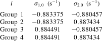
whose solutions are shown in table 2. Since $\unicode[STIX]{x1D70E}_{1,0}$ , $\unicode[STIX]{x1D70E}_{2,0}$ must be positive, only group 4 has physical meaning. As long as $\unicode[STIX]{x1D70E}_{1,0}$ , $\unicode[STIX]{x1D70E}_{2,0}$ are determined, $\unicode[STIX]{x1D711}_{0}$ is known. And, with the initial guess $\unicode[STIX]{x1D702}_{0}=0$ , it is straightforward to calculate $\unicode[STIX]{x1D702}_{1}$ directly. We have

(3.9) $$\begin{eqnarray}\displaystyle \unicode[STIX]{x1D702}_{1} & = & \displaystyle c_{0}\unicode[STIX]{x1D6E5}_{0}^{\unicode[STIX]{x1D702}}\nonumber\\ \displaystyle & = & \displaystyle \overline{a}_{1,0}\cos (\unicode[STIX]{x1D709}_{1})+\overline{a}_{0,1}\cos (\unicode[STIX]{x1D709}_{2})+\overline{a}_{1,1}\cos (\unicode[STIX]{x1D709}_{1}+\unicode[STIX]{x1D709}_{2})\nonumber\\ \displaystyle & & \displaystyle +\,\overline{a}_{2,1}\cos (2\unicode[STIX]{x1D709}_{1}+\unicode[STIX]{x1D709}_{2})+\overline{a}_{1,2}\cos (\unicode[STIX]{x1D709}_{1}+2\unicode[STIX]{x1D709}_{2}),\end{eqnarray}$$

where $\overline{a}_{m_{1},m_{2}}$ are known constants.

Now, all terms on the right-hand side of the first-order deformation equation (2.29) ( $m=1$ ) are known, so it is straightforward to obtain $\unicode[STIX]{x1D711}_{1}$ :

(3.10) $$\begin{eqnarray}\displaystyle \unicode[STIX]{x1D711}_{1}={\mathcal{L}}^{\ast -1}[c_{0}\unicode[STIX]{x1D6E5}_{0}^{\unicode[STIX]{x1D711}}-\bar{S}_{1}]+A^{\ast }\unicode[STIX]{x1D6F9}_{1,0}+B^{\ast }\unicode[STIX]{x1D6F9}_{0,1}. & & \displaystyle\end{eqnarray}$$

Since the components $A(\unicode[STIX]{x1D714}/g)\unicode[STIX]{x1D6F9}_{1,0}$ and $B(\unicode[STIX]{x1D714}/g)\unicode[STIX]{x1D6F9}_{0,1}$ of the two primary waves are given, we have $A^{\ast }=B^{\ast }=0$ so that

(3.11) $$\begin{eqnarray}\displaystyle \unicode[STIX]{x1D711}_{1} & = & \displaystyle {\mathcal{L}}^{\ast -1}[c_{0}\unicode[STIX]{x1D6E5}_{0}^{\unicode[STIX]{x1D711}}-\bar{S}_{1}]\nonumber\\ \displaystyle & = & \displaystyle \overline{d}_{1,0}\unicode[STIX]{x1D6F9}_{1,0}+\overline{d}_{0,1}\unicode[STIX]{x1D6F9}_{0,1}+\overline{d}_{2,0}\unicode[STIX]{x1D6F9}_{2,0}+\overline{d}_{0,2}\unicode[STIX]{x1D6F9}_{0,2}+\overline{d}_{1,1}\unicode[STIX]{x1D6F9}_{1,1}+\overline{d}_{1,-1}\unicode[STIX]{x1D6F9}_{1,-1}+\overline{d}_{2,1}\unicode[STIX]{x1D6F9}_{2,1}\nonumber\\ \displaystyle & & \displaystyle +\,\overline{d}_{1,2}\unicode[STIX]{x1D6F9}_{1,2}+\overline{d}_{3,1}\unicode[STIX]{x1D6F9}_{3,1}+\overline{d}_{2,2}\unicode[STIX]{x1D6F9}_{2,2}+\overline{d}_{1,3}\unicode[STIX]{x1D6F9}_{1,3}+\overline{d}_{3,2}\unicode[STIX]{x1D6F9}_{3,2}+\overline{d}_{2,3}\unicode[STIX]{x1D6F9}_{2,3}+\overline{d}_{3,3}\unicode[STIX]{x1D6F9}_{3,3},\end{eqnarray}$$

where $\overline{d}_{m_{1},m_{2}}=\overline{b}_{m_{1},m_{2}}/\tilde{\unicode[STIX]{x1D706}}_{m_{1},m_{2}}^{\ast }$ . We substitute $\unicode[STIX]{x1D711}_{1}$ into the second-order deformation equation (2.29) ( $m=2$ ). Note that coefficients of $\sin (m_{1}\unicode[STIX]{x1D709}_{1}+m_{2}\unicode[STIX]{x1D709}_{2})$ contain $\unicode[STIX]{x1D70E}_{1,1}$ and $\unicode[STIX]{x1D70E}_{2,1}$ that are unknown right now. Then, enforcing the coefficients of $\sin (\unicode[STIX]{x1D709}_{1})$ and $\sin (\unicode[STIX]{x1D709}_{2})$ on its right-hand side to be zero so as to avoid secular terms, we can further determine $\unicode[STIX]{x1D70E}_{1,1}$ and $\unicode[STIX]{x1D70E}_{2,1}$ in a similar way. Then, we can similarly obtain $\unicode[STIX]{x1D702}_{2}$ , $\unicode[STIX]{x1D711}_{2}$ , and so on.

In addition, the ‘convergence-control parameter’ $c_{0}$ can provide a convenient way to guarantee the convergence of the solution series in the framework of HAM. The optimal value of $c_{0}$ is determined through the minimum residuals of (2.12) and (2.13) to guarantee the convergence of the HAM approximations. Define the averaged residual square as

(3.12) $$\begin{eqnarray}\displaystyle & \displaystyle \unicode[STIX]{x1D700}_{m}^{\unicode[STIX]{x1D719}}=\frac{1}{\unicode[STIX]{x03C0}^{2}}\int _{0}^{\unicode[STIX]{x03C0}}\int _{0}^{\unicode[STIX]{x03C0}}\left(\mathop{\sum }_{n=0}^{m}\unicode[STIX]{x1D6E5}_{n}^{\unicode[STIX]{x1D719}}\right)^{2}\,\text{d}\unicode[STIX]{x1D709}_{1}\,\text{d}\unicode[STIX]{x1D709}_{2}, & \displaystyle\end{eqnarray}$$

(3.13) $$\begin{eqnarray}\displaystyle & \displaystyle \unicode[STIX]{x1D700}_{m}^{\unicode[STIX]{x1D702}}=\frac{1}{\unicode[STIX]{x03C0}^{2}}\int _{0}^{\unicode[STIX]{x03C0}}\int _{0}^{\unicode[STIX]{x03C0}}\left(\mathop{\sum }_{n=0}^{m}\unicode[STIX]{x1D6E5}_{n}^{\unicode[STIX]{x1D702}}\right)^{2}\,\text{d}\unicode[STIX]{x1D709}_{1}\,\text{d}\unicode[STIX]{x1D709}_{2}, & \displaystyle\end{eqnarray}$$

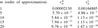
for the $m$ th-order approximation of $\unicode[STIX]{x1D719}$ and $\unicode[STIX]{x1D702}$ . The residual errors of $\unicode[STIX]{x1D700}_{m}^{\unicode[STIX]{x1D719}}$ and $\unicode[STIX]{x1D700}_{m}^{\unicode[STIX]{x1D702}}$ both decrease sharply when the value of $c_{0}$ is close to $-1.35$ , as shown in figure 1. Then, we choose $c_{0}=-1.35$ . 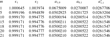The corresponding residual error squares of the two boundary conditions decease rather quickly to the level $10^{-16}$ at 20th order, as shown in table 3 and figure 2. Then, we can obtain the convergent wave frequencies and amplitudes, which are given in table 4. The $a_{1,1}^{\ast }$ represents the amplitude corresponding to the resonant hydroacoustic wave component. If we neglect the $g(\unicode[STIX]{x2202}\unicode[STIX]{x1D711}/\unicode[STIX]{x2202}z)$ term in (2.1), we can also get the convergent series solutions of the steady-state resonant acoustic–gravity waves, as shown in table 5. It is found that the gravity contribution in (2.1) is very small. The existence of $g(\unicode[STIX]{x2202}\unicode[STIX]{x1D711}/\unicode[STIX]{x2202}z)$ has negligible effect on the calculation results of this paper. Actually, one can omit the gravity contribution in (2.1) for practical purposes. This conclusion was also confirmed by Abdolali & Kirby (Reference Abdolali and Kirby2017), who showed the negligible role of $g(\unicode[STIX]{x2202}\unicode[STIX]{x1D711}/\unicode[STIX]{x2202}z)$ on hydroacoustic waves and surface gravity waves with short wavelength. Furthermore, we investigate different cases in a similar way, as shown in table 6.

Figure 1.

Averaged residual squares versus $c_{0}$ in the case of $h=4000~\text{m}$ , $k_{1}=k_{2}=0.0796449~\text{m}^{-1}$ , $A=1/20~\text{m}$ , $B=1/50~\text{m}$ , $C=1/50~\text{m}$ . Solid line: first-order approximation; dashed line: third-order approximation; dash-dot-dotted line: fifth-order approximation; dotted line: seventh-order approximation. Panel (a) represents averaged residual square of $\log _{10}\unicode[STIX]{x1D700}_{m}^{\unicode[STIX]{x1D719}}$ versus $c_{0}$ and (b) represents averaged residual square of $\log _{10}\unicode[STIX]{x1D700}_{m}^{\unicode[STIX]{x1D702}}$ versus $c_{0}$ .

Table 3.

The averaged residual squares of $\unicode[STIX]{x1D700}_{m}^{\unicode[STIX]{x1D719}}$ and $\unicode[STIX]{x1D700}_{m}^{\unicode[STIX]{x1D702}}$ in the case of $h=4000~\text{m}$ , $k_{1}=k_{2}=0.0796449~\text{m}^{-1}$ , $A=1/20~\text{m}$ , $B=1/50~\text{m}$ , $C=1/50~\text{m}$ by means of $c_{0}=-1.35$ .

Figure 2.

Averaged residual squares of $\unicode[STIX]{x1D700}_{m}^{\unicode[STIX]{x1D719}}$ and $\unicode[STIX]{x1D700}_{m}^{\unicode[STIX]{x1D702}}$ versus the approximation order $m$ by means of $c_{0}=-1.35$ in the case of $h=4000~\text{m}$ , $k_{1}=k_{2}=0.0796449~\text{m}^{-1}$ , $A=1/20~\text{m}$ , $B=1/50~\text{m}$ , $C=1/50~\text{m}$ .

Figure 3.

Time variation of dynamic pressure ( $p_{d}$ ) induced by the resulting hydroacoustic wave in the case $k_{1}=k_{2}=0.0796449~\text{m}^{-1}$ , $A=1/20~\text{m}$ , $B=1/50~\text{m}$ , $C=1/50~\text{m}$ .

Table 4.

Analytical approximations of the dimensional angular frequencies and wave amplitude components (m) in the case of $k_{1}=k_{2}=0.0796449~\text{m}^{-1}$ , $A=1/20~\text{m}$ , $B=1/50~\text{m}$ , $C=1/50~\text{m}$ .

Table 5.

The dimensionless angular frequencies and the wave amplitude components (m) in the case with $|\boldsymbol{k}_{3}|=0$ (mode $n=1$ ),  $A=1/20~\text{m}$ and $B=1/50~\text{m}$ with or without the $g(\unicode[STIX]{x2202}\unicode[STIX]{x1D711}/\unicode[STIX]{x2202}z)$ term in (2.1).

Table 6.

The dimensionless angular frequencies and the wave amplitude components (m) versus $A$ (m) and $B$ (m) in the case of $k_{1}=k_{2}=0.0796449~\text{m}^{-1}$ .

Table 7.

The energy distribution of the wave system versus $A$ (m) and $B$ (m) in the case of $k_{1}=k_{2}=0.0796449~\text{m}^{-1}$ .

Define

(3.14) $$\begin{eqnarray}\displaystyle \unicode[STIX]{x1D6F1}=\mathop{\sum }_{m_{1}=0}^{+\infty }\mathop{\sum }_{m_{2}=-\infty }^{+\infty }(a_{m_{1},m_{2}})^{2}. & & \displaystyle\end{eqnarray}$$

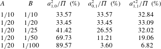
The wave amplitudes and energy distributions of the two primary waves and resonant hydroacoustic wave component are given in table 7. It is found that the two primary gravity waves and the resonant hydroacoustic wave as a whole occupy most wave energy in all considered cases. A similar conclusion was found for steady-state exactly/nearly resonant gravity waves by Liao (Reference Liao2011b ), Xu et al. (Reference Xu, Lin, Liao and Stiassnie2012), Liu & Liao (Reference Liu and Liao2014), Liu et al. (Reference Liu, Xu, Li, Peng, Alsaedi and Liao2015) and Liao et al. (Reference Liao, Xu and Stiassnie2016).

Next, we discuss the pressure distribution of the steady-state resonant acoustic–gravity waves. We consider here the dynamic pressure $p_{d}$ of the resulting hydroacoustic wave in the whole fluid. Figure 3 shows the time variation of dynamic pressure ( $p_{d}$ ) induced by the hydroacoustic wave in the case $k_{1}=k_{2}=0.0796449~\text{m}^{-1}$ , $A=1/20~\text{m}$ , $B=1/50~\text{m}$ . It is found that, when the resonance condition is exactly satisfied, acoustic–gravity waves can also generate a periodic pressure on the ocean floor, whose frequency is the superposition of the actual wave frequencies of the two primary waves. If the amplitudes of the two primary waves are the same (the cases corresponding to $A=B$ in the initial guess $\unicode[STIX]{x1D711}_{0}$ ), the actual wave frequencies of the two primary waves are the same. So, the frequency of the pressure at the sea bottom is exactly twice the wave frequency of the primary gravity waves. The pressure generated by the acoustic–gravity waves is dependent of the water depth, as shown in figure 3. The magnitude of pressure is related to the amplitude of the hydroacoustic wave, which is determined by the value of $A$ and $B$ in the initial guess of the velocity potential $\unicode[STIX]{x1D711}_{0}$ . In the present case, the maximum dynamic pressure on the bottom is approximately 70 kPa, which is much larger than the pressure ( ${\approx}3.5~\text{Pa}$ ) obtained in the above-mentioned case of non-resonance with the same amplitude $A=1/20~\text{m}$ and $B=1/50~\text{m}$ of the velocity potential $\unicode[STIX]{x1D711}_{0}$ . This value is of the same order of magnitude as the maximum dynamic pressure of the first acoustic–gravity wave mode generated by bottom motion in the study of Oliveira & Kadri (Reference Oliveira and Kadri2016). So, the resonant acoustic–gravity waves might indeed trigger microseisms in the Earth.

Figure 4.

The second-order pressure induced by two opposite primary waves in the case of $\unicode[STIX]{x1D714}_{1}=0.884266~\text{s}^{-1}$ , $a_{1,0}=0.0500210~\text{m}$ , $a_{0,1}=0.0200522~\text{m}$ .

Without considering the compressibility of the water, Pellet et al. (Reference Pellet, Christodoulides, Donne, Bean and Dias2017) obtained a second-order pressure field generated by two exactly opposite travelling gravity waves ( $\boldsymbol{k}_{1}+\boldsymbol{k}_{2}=\mathbf{0}$ ), which is independent of water depth and periodic in time with twice the frequency of the primary gravity waves. It reads

(3.15) $$\begin{eqnarray}\displaystyle p_{2}=8\unicode[STIX]{x1D70C}\unicode[STIX]{x1D714}_{1}^{2}a_{1,0}a_{0,1}\cos (2\unicode[STIX]{x1D714}_{1}t). & & \displaystyle\end{eqnarray}$$

We choose the same amplitudes of the two primary waves as these in the resonance case (3.6). $a_{1,0}=0.0500210~\text{m},a_{0,1}=0.0200522~\text{m}$ . Then we can get the second-order pressure field, as shown in figure 4. The second-order pressure is proportional to the amplitudes of the two primary waves. It is found that when the acoustic–gravity waves resonance occurs, the maximum dynamic pressure on the bottom is approximately 70 kPa (with compressibility), which is much larger than the second-order pressure ( ${\approx}6~\text{Pa}$ ) (without compressibility) obtained with the same amplitudes of the two primary waves. The reason is that no resonance occurs in the whole system, when we ignore the compressibility of water.

3.2.2 Resonant waves for the case with $|\boldsymbol{k}_{3}|=0$ (mode $n=2$ )

Here, we investigate the following resonant acoustic–gravity wave system (mode $n=2$ ):

(3.16a ) $$\begin{eqnarray}\displaystyle & \displaystyle \boldsymbol{k}_{1}=(0.221124,0)~\text{m}^{-1},\quad \unicode[STIX]{x1D714}_{1}=1.47283~\text{s}^{-1}, & \displaystyle\end{eqnarray}$$

(3.16b ) $$\begin{eqnarray}\displaystyle & \displaystyle \boldsymbol{k}_{2}=(-0.221124,0)~\text{m}^{-1},\quad \unicode[STIX]{x1D714}_{2}=1.47283~\text{s}^{-1}, & \displaystyle\end{eqnarray}$$

(3.16c ) $$\begin{eqnarray}\displaystyle & \displaystyle \boldsymbol{k}_{3}=(0,0)~\text{m}^{-1},\quad \unicode[STIX]{x1D714}_{3}=2.94566~\text{s}^{-1}. & \displaystyle\end{eqnarray}$$

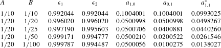
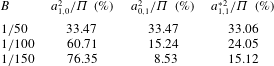
In this case, we choose $A=1/50~\text{m}$ and different values of $B$ in the initial guess (2.47). The dimensionless angular frequencies and the wave amplitude components in different conditions are shown in table 8. Similarly to the results of case (3.6), it is found that the two primary gravity waves and the resonant hydroacoustic wave as a whole occupy most wave energy in all considered cases, as shown in table 9. The dynamic pressure $p_{d}$ of the resulting hydroacoustic wave in the whole fluid in the case of $A=1/50~\text{m}$ and $B=1/100~\text{m}$ is shown in figure 5. The maximum dynamic pressure on the bottom is approximately 55 kPa, which might indeed trigger microseisms of the ocean floor.

Figure 5.

Time variation of dynamic pressure ( $p_{d}$ ) induced by the resulting hydroacoustic wave in the case $k_{1}=k_{2}=0.221124~\text{m}^{-1}$ , $A=1/50~\text{m}$ , $B=1/100~\text{m}$ .

Table 8.

The dimensionless angular frequencies and the wave amplitude components (m) versus $B$ (m) in the case of $k_{1}=k_{2}=0.221124~\text{m}^{-1}$ , $A=1/50~\text{m}$ .

Table 9.

The energy distribution of the wave system versus $B$ (m) in the case of $k_{1}=k_{2}=0.221124~\text{m}^{-1}$ , $A=1/50~\text{m}$ .

3.2.3 Resonant waves for the case with $0<|\boldsymbol{k}_{3}|<\unicode[STIX]{x1D714}_{3}/c$

The resonance case (mode $n=1$ ) given by Kadri & Stiassnie (Reference Kadri and Stiassnie2013) is

(3.17a ) $$\begin{eqnarray}\displaystyle & \displaystyle \boldsymbol{k}_{1}=(0.102249,0)~\text{m}^{-1},\quad \unicode[STIX]{x1D714}_{1}=1.00153~\text{s}^{-1}, & \displaystyle\end{eqnarray}$$

(3.17b ) $$\begin{eqnarray}\displaystyle & \displaystyle \boldsymbol{k}_{2}=(-0.101625,0)~\text{m}^{-1},\quad \unicode[STIX]{x1D714}_{2}=0.99847~\text{s}^{-1}, & \displaystyle\end{eqnarray}$$

(3.17c ) $$\begin{eqnarray}\displaystyle & \displaystyle \boldsymbol{k}_{3}=(0.000642,0)~\text{m}^{-1},\quad \unicode[STIX]{x1D714}_{3}=2.00000~\text{s}^{-1}. & \displaystyle\end{eqnarray}$$

For studying this resonance case, we choose $A=1/20~\text{m}$ and different values of $B$ in the initial guess (2.47). We can obtain the convergent wave frequencies and amplitudes through the same calculation process as in § 3.2.1, as shown in table 10. The energy distributions of the wave system are shown in table 11. It is found that the convergent solutions of the resonance steady-state acoustic–gravity triads for general resonance case with $0<|\boldsymbol{k}_{3}|<\unicode[STIX]{x1D714}_{3}/c$ can even be obtained. This illustrates the generality of the existence of the steady-state resonant acoustic–gravity waves. And the two primary gravity waves along with the resonant hydroacoustic wave as a whole occupy most wave energy in the wave system like (3.6) and (3.16) with $|\boldsymbol{k}_{3}|=0$ .

Table 10.

The dimensionless angular frequencies and the wave amplitude components (m) versus $B$ (m) in the case of $k_{1}=0.102249~\text{m}^{-1}$ , $k_{2}=0.101625~\text{m}^{-1}$ , $A=1/20~\text{m}$ .

Table 11.

The energy distribution of the wave system versus $B$ (m) in the case of $k_{1}=0.102249~\text{m}^{-1}$ , $k_{2}=0.101625~\text{m}^{-1}$ , $A=1/20~\text{m}$ .

Even in the cases of $h=2000~\text{m}$ and $h=3000~\text{m}$ , we also obtain the steady-state resonant acoustic–gravity waves. It means that steady-state resonant acoustic–gravity waves commonly exist in water of uniform depth. This agrees with Kadri & Stiassnie (Reference Kadri and Stiassnie2013), who pointed out that the water depth $h$ should be greater than $h_{cr}\equiv \unicode[STIX]{x03C0}c/2\unicode[STIX]{x1D714}_{3}$ for the existence of a hydroacoustic wave.