1 Introduction
Investigation into the propagation of detonation in the presence of momentum and heat losses began in the 1940s with the seminal work by Zel’dovich (Reference Zel’dovich1940) and then by Schelkin (Reference Schelkin1949). Such losses arise when gaseous detonation propagates in small tubes (e.g. Zel’dovich et al. Reference Zel’dovich, Gel’fand, Kazhdan and Frolov1987; Chan & Greig Reference Chan and Greig1989; Manzhalei Reference Manzhalei1992; Camargo et al. Reference Camargo, Ng, Chao and Lee2010), narrow channels (e.g. Manzhalei Reference Manzhalei1998; Ishii & Monwar Reference Ishii and Monwar2011; Gao, Ng & Lee Reference Gao, Ng and Lee2017), channels with obstructions (e.g. Lee, Knystautas & Freiman Reference Lee, Knystautas and Freiman1984; Lee, Knystautas & Chan Reference Lee, Knystautas and Chan1985; Chan & Greig Reference Chan and Greig1989; Teodorczyk, Lee & Knystautas Reference Teodorczyk, Lee and Knystautas1989, Reference Teodorczyk, Lee and Knystautas1991; Gao et al. Reference Gao, Ng and Lee2017), packed beds of inert particles (e.g. Lyamin & Pinaev Reference Lyamin and Pinaev1985; Babkin, Korzhavin & Bunev Reference Babkin, Korzhavin and Bunev1991; Lyamin et al. Reference Lyamin, Mitrofanov, Pinaev and Subbotin1991; Makris et al. Reference Makris, Shafique, Lee and Knystautas1995; Babkin Reference Babkin2012) or tubes with porous walls (Radulescu & Lee Reference Radulescu and Lee2002). Friction with and heat transfer to the walls or obstacles (or the mass loss through the porous walls) decreases the velocity of detonation from its ideal value (i.e. there exists a velocity deficit). The mechanisms causing this velocity deficit are not well understood. The stable propagation of low-velocity detonation (LVD) is of particular interest, whereby propagation from near acoustic speeds to speeds of approximately half the ideal velocity are observed. Detonation propagating at a velocity above this range, but below the ideal value, is termed ‘quasi-detonation’. The regime of its propagation at a velocity near the sound speed in the burnt gases is termed ‘sonic’ or ‘choking’ (Lee Reference Lee2008). Extensive efforts aimed at explaining these phenomena are reviewed in Gelfand, Frolov & Nettleton (Reference Gelfand, Frolov and Nettleton1991), Ciccarelli & Dorofeev (Reference Ciccarelli and Dorofeev2008), Lee (Reference Lee2008), Brailovsky, Kagan & Sivashinsky (Reference Brailovsky, Kagan and Sivashinsky2012).
The simplest theoretical analysis of detonation with losses follows the formulation by Zel’dovich (Reference Zel’dovich1940), which is based on the one-dimensional (1-D) reactive Euler equations modified to account for momentum and heat losses. In qualitative agreement with experiments, the analysis predicts that these losses lead to a velocity deficit. In most previous works, a reverse
 $S$
shaped dependence of the detonation velocity,
 $D$
, on the loss coefficient,
 $c_{f}$
, has been derived (Zel’dovich & Kompaneets Reference Zel’dovich and Kompaneets1960; Zel’dovich et al.
Reference Zel’dovich, Gel’fand, Kazhdan and Frolov1987; Brailovsky & Sivashinsky Reference Brailovsky and Sivashinsky2000, Reference Brailovsky and Sivashinsky2002; Brailovsky et al.
Reference Brailovsky, Kagan and Sivashinsky2012; Higgins Reference Higgins2012). The top branch of the
 $D$
–
 $c_{f}$
curve corresponding to small velocity deficits is generally stable and attracting. Even in the presence of hydrodynamic instabilities, the average propagation velocity remains in the vicinity of the top branch (Zhang & Lee Reference Zhang and Lee1994; Dionne, Ng & Lee Reference Dionne, Ng and Lee2000). The middle branch is always found to be a repeller, such that solutions starting near that branch tend toward the top branch or fail. For this reason, the solutions corresponding to the middle branch have been considered unphysical and often not computed (e.g. Zel’dovich et al.
Reference Zel’dovich, Gel’fand, Kazhdan and Frolov1987; Dionne et al.
Reference Dionne, Ng and Lee2000). It should be noted that LVDs observed in experiments often propagate stably at rather low velocities (e.g. Lyamin et al.
Reference Lyamin, Mitrofanov, Pinaev and Subbotin1991) that are likely to correspond to the unstable middle branch of theoretical predictions (However, to the best of our knowledge, no such direct comparison is available in the literature.). This apparent discrepancy raises an important question about the physical reasons for the observed stability of the LVD. In this connection, one could question the applicability of the 1-D modelling of this phenomenon, especially so in view of the complex multi-dimensional flow structures observed in experiments. In this paper, we show evidence of a mechanism that provides stability to the lower-branch solutions within the 1-D approximation.
Various possible mechanisms (not necessarily mutually exclusive) have previously been proposed to explain LVD. One involves a fast turbulent deflagration that propagates at a speed near the sound speed in the products. Flames at such high speeds are presumably promoted by the large area of the flame caused by the turbulence in the flow between the lead shock and the deflagration front (Lee et al. Reference Lee, Knystautas and Freiman1984, Reference Lee, Knystautas and Chan1985; Teodorczyk et al. Reference Teodorczyk, Lee and Knystautas1989, Reference Teodorczyk, Lee and Knystautas1991; Ciccarelli & Dorofeev Reference Ciccarelli and Dorofeev2008; Lee Reference Lee2008). In Manzhalei (Reference Manzhalei1992, Reference Manzhalei1999), it is suggested that the two-dimensional structure of the flame plays an important role in providing the necessary level of coupling between the lead shock and the flame. Another mechanism assigns a key role to frictional heating of the gas between the lead shock and the deflagration wave (see e.g. Babkin et al. Reference Babkin, Korzhavin and Bunev1991; Korzhavin et al. Reference Korzhavin, Bunev, Babkin, Lawes and Bradley1999; Babkin Reference Babkin2012 and the review Brailovsky et al. Reference Brailovsky, Kagan and Sivashinsky2012) while the multi-dimensional and turbulent phenomena are assumed to contribute in some averaged sense and be represented through the momentum and heat-loss coefficients.
As mentioned, the 1-D predictions appear to contradict the observed stability of LVD because of the unconditional instability of the middle branch of the
 $D$
–
 $c_{f}$
curve. A recent analysis of gaseous detonation in a porous medium with both momentum and heat losses shows that instead of the reversed
 $S$
shaped dependence, the set of solutions in the
 $D$
–
 $c_{f}$
plane contains a region filled with a continuum of solutions at low velocities (Semenko et al.
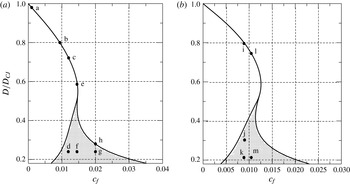
Reference Semenko, Faria, Kasimov and Ermolaev2016) (see figure 1). For a given mixture and fixed
 $c_{f}$
, there is a finite and continuous range of detonation velocities at which steady solutions exist. This peculiarity of the solutions points to an intriguing possibility of the existence of a stable detonation in a wide range of low velocities. Indeed, any particular solution inside the set-valued region is not isolated, but is surrounded by a continuum of other steady-state solutions. Therefore, a small perturbation to such a steady solution can be expected to simply shift the solution to a neighbouring one. To illustrate this picture, one could draw the following mechanical analogy with a particle moving in a potential energy field: the top and the middle branches of the reversed
 $S$
shaped dependence are analogous to a potential minimum (stable) and maximum (unstable), respectively. The set-valued region is then analogous to a flat maximum, and hence it is a neutrally stable equilibrium. Any solution that starts in the set-valued region can be expected to remain in the neighbourhood of its initial condition for a long time. That this is indeed the case is demonstrated by the computations below.
Dependence of the detonation speed on the loss factor at (a)
 $E=25$
and (b)
 $E=27$
. In both cases,
 $Q=50$
,
 $\unicode[STIX]{x1D6FE}=1.2$
and
 $c_{h}=0.4c_{f}$
.

The existence of (at least neutrally) stable solutions at low velocities is investigated by solving the reactive Euler equations including momentum and heat losses with initial conditions taken as the steady travelling wave solutions of the system. In other words, we analyse the nonlinear stability of the solutions obtained in Semenko et al. (Reference Semenko, Faria, Kasimov and Ermolaev2016). Our main finding is that the steady solutions inside the set-valued region are long lived, as expected, and either transition to the top-branch pulsating regimes or fail over very long times, confirming our expectation of increased stability of low-velocity detonations. We show that during the transition from LVD to pulsating solutions, the lead shock and the deflagration front propagate at nearly the same speed in an almost steady manner for a substantial length of time before a rapid transition takes place.
The remainder of the paper is organized as follows. In § 2, we introduce the reactive Euler equations that include momentum and heat exchange terms and briefly explain the numerical algorithm. In § 3, we present the steady-state solutions and in § 4, we present the main computational results. In § 5, we discuss the mechanism of the initial slow acceleration of the wave and its transition to the upper-branch solutions. Concluding remarks are offered in § 6.
2 Governing equations and the numerical method
We consider a model describing a reactive perfect gas filling the interstitial space of a packed bed of solid inert particles. The heat release is assumed to follow a one-step global mechanism and the losses to be described by algebraic functions
 $f$
for momentum and
 $h$
for heat. Then, the reactive Euler equations take the form (Semenko et al.
Reference Semenko, Faria, Kasimov and Ermolaev2016)
 $$\begin{eqnarray}\left.\begin{array}{@{}c@{}}\displaystyle \unicode[STIX]{x1D70C}_{t}+(\unicode[STIX]{x1D70C}u)_{x}=0,\\ \displaystyle (\unicode[STIX]{x1D70C}u)_{t}+(\unicode[STIX]{x1D70C}u^{2}+p)_{x}=-f/\unicode[STIX]{x1D719},\\ \displaystyle (\unicode[STIX]{x1D70C}{\mathcal{E}})_{t}+(\unicode[STIX]{x1D70C}u{\mathcal{E}}+pu)_{x}=-h/\unicode[STIX]{x1D719},\\ \displaystyle (\unicode[STIX]{x1D70C}\unicode[STIX]{x1D706})_{t}+(\unicode[STIX]{x1D70C}u\unicode[STIX]{x1D706})_{x}=\unicode[STIX]{x1D70C}\unicode[STIX]{x1D714},\end{array}\right\}\end{eqnarray}$$
where
 $\unicode[STIX]{x1D70C}$
,
 $u$
,
 $p$
and
 $\unicode[STIX]{x1D706}$
are the density, flow velocity, pressure and reaction progress variable, respectively, while
 $\unicode[STIX]{x1D719}$
denotes the medium porosity. Variable
 $\unicode[STIX]{x1D706}$
varies between
 $0$
in reactants to
 $1$
in products. The total energy density is
 ${\mathcal{E}}=p/\left(\unicode[STIX]{x1D70C}\left(\unicode[STIX]{x1D6FE}-1\right)\right)+u^{2}/2-\unicode[STIX]{x1D706}Q$
with
 $Q$
denoting the heat release and
 $\unicode[STIX]{x1D6FE}$
the ratio of specific heats. The ideal gas equation of state is assumed. The reaction rate is of the Arrhenius form,
 $\displaystyle \unicode[STIX]{x1D714}=k\left(1-\unicode[STIX]{x1D706}\right)\exp \left(-E/RT\right)$
, with
 $k$
denoting the rate constant,
 $R$
the universal gas constant and
 $E$
the activation energy. The governing equations are rescaled with respect to the upstream state,
 $\unicode[STIX]{x1D70C}_{a},$
 $p_{a}$
and
 $u_{a}=\sqrt{p_{a}/\unicode[STIX]{x1D70C}_{a}}$
. The length scale is chosen to be the half-reaction zone length,
 $l_{1/2}$
, of the ideal planar detonation, and the time scale is
 $l_{1/2}/u_{a}$
. The drag force and heat-loss terms are assumed to follow the same modelling assumptions as in Semenko et al. (Reference Semenko, Faria, Kasimov and Ermolaev2016) and are taken as
 $f=c_{f}\unicode[STIX]{x1D70C}u\left|u\right|$
and
 $h=c_{h}\left|u\right|\left(T-1\right)$
. Here, the dimensionless coefficients
 $c_{f}$
and
 $c_{h}$
depend on a large number of physical parameters that describe the gas transport properties, the porous medium and the chemical reactions, as the reader can find in Semenko et al. (Reference Semenko, Faria, Kasimov and Ermolaev2016). In particular, using the assumptions of Semenko et al. (Reference Semenko, Faria, Kasimov and Ermolaev2016), that the Reynolds number is large and taking
 $\unicode[STIX]{x1D719}=0.4$
, we obtain that
 $c_{f}=2.7\,l_{1/2}/d$
, where
 $d$
is the particle diameter. Following the same reference, it is assumed that
 $c_{h}=0.4c_{f}$
and therefore
 $c_{f}$
remains the only parameter characterizing the losses.
For the numerical solution of the above system, we have implemented a shock-fitting algorithm based on a fifth-order finite difference WENO5M (weighted essentially non-oscillatory) scheme for the spatial discretization and a fifth-order Runge–Kutta method for the temporal integration (Henrick, Aslam & Powers Reference Henrick, Aslam and Powers2006). As in Henrick et al. (Reference Henrick, Aslam and Powers2006), the shock change equation was derived and discretized to compute the detonation velocity. However, unlike Henrick et al. (Reference Henrick, Aslam and Powers2006), biased approximations of spatial derivatives near the shock were not used to avoid numerical stability problems when secondary shocks that frequently arise in the reaction zone interact with the lead shock. The lead shock state was extrapolated ahead of the detonation shock whenever necessary, which had a drawback of reducing the order of the method to first, but gave the advantage of a numerical stability under a wide range of conditions. The spatial discretization of the physical domain was based on a uniform Cartesian grid.
A particular challenge for the present computations is related to the extreme range of spatial scales often present in simulations and very long computational times that are often necessary. Parallel computer resources were required in most cases, especially in the low-velocity regimes. Up to
 $200$
processor cores were used. Numerical resolutions were
 $N_{1/2}=50$
,
 $N_{1/2}=100$
or
 $N_{1/2}=200$
, where
 $N_{1/2}$
denotes the number of grid points per unit length. The domain lengths used were between
 $L=100$
and
 $L=4000$
depending on a particular case. At the downstream boundary, the flow variables were extrapolated. We assured that neither the resolution nor the domain length had an appreciable effect on the results.
3 Steady-state solutions
Steady travelling wave solutions of (2.1) were thoroughly investigated in Semenko et al. (Reference Semenko, Faria, Kasimov and Ermolaev2016). It was found that solutions exist with wave speeds,
 $D$
, that can vary from the ideal (Chapman–Jouguet) value,
 $D_{CJ}$
, down to the ambient sound speed,
 $c_{a}=\sqrt{\unicode[STIX]{x1D6FE}}$
. At each wave speed, the solution exists only at a particular value (or range) of
 $c_{f}$
. These results are consistent with previous findings (e.g. Zel’dovich & Kompaneets Reference Zel’dovich and Kompaneets1960; Zel’dovich et al.
Reference Zel’dovich, Gel’fand, Kazhdan and Frolov1987; Brailovsky & Sivashinsky Reference Brailovsky and Sivashinsky2002). However, a peculiar feature of the
 $D$
–
 $c_{f}$
dependence, revealed for the first time in Semenko et al. (Reference Semenko, Faria, Kasimov and Ermolaev2016), is the presence of a set-valued region, i.e. a continuous range of
 $D$
for a given
 $c_{f}$
at sufficiently low wave speeds, shown in figure 1 as a shaded region. These solutions exist only with both momentum and heat losses and correspond to the postshock flow without a sonic locus. They are also accompanied by a flow reversal effect such that in some part of the postshock flow, the gas moves opposite to the direction of the wave in the laboratory frame of reference. Two examples of
 $D$
–
 $c_{f}$
dependence at two different activation energies are shown in figure 1. The steady-state solutions exist at every pair of (
 $D$
,
 $c_{f}$
) on the curves as well as inside the shaded regions. In table 1, we list the coordinates of the labelled points in figure 1. Stability of solutions corresponding to these points is investigated below.
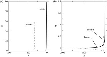
Profiles of the steady-state reaction rate (a) and fluid velocity (b) at points c and d on figure 1(a).

Values of
 $D/D_{CJ}$
and
 $c_{f}$
at points indicated in figure 1.

To contrast the nature of the steady-state solutions that coexist at the same value of
 $c_{f}$
, we show in figure 2 the profiles of the reaction rate and flow velocity at points c and d. Note that the velocity profile at d, the point inside the set-valued region, has a substantial negative phase. As explained in Semenko et al. (Reference Semenko, Faria, Kasimov and Ermolaev2016), such flow reversal is only possible in the presence of heat losses. What is also important in these figures is that the solutions in the set-valued region have a very sharp ‘fire’ located far from the lead shock (figure 2
a) and a very long velocity relaxation region downstream of the fire (figure 2
b). Corresponding temperature profiles (not shown here) also exhibit striking contrast (Semenko et al.
Reference Semenko, Faria, Kasimov and Ermolaev2016). At point c, the shock is strong enough to raise the gas temperature to sufficiently high levels so as to ignite the gas, and hence this structure and the wave propagation mechanism are close to those of the ideal case. In contrast, at point d, the lead shock is weak and the shock temperature is insufficient to initiate reactions. Instead, the temperature is raised by frictional heating in the region between the shock and the ‘fire’. A more detailed discussion of these effects can be found in Semenko et al. (Reference Semenko, Faria, Kasimov and Ermolaev2016).
4 Nonlinear stability results
In this section, we explore the stability of the steady-state solutions indicated by points in figure 1. These solutions are taken as initial conditions in the simulations. Their instability is triggered by numerical discretization errors. Note that the ideal detonation at
 $E=25$
is stable while that at
 $E=27$
is unstable with respect to one-dimensional perturbations (Lee & Stewart Reference Lee and Stewart1990).
The presence of losses leads to the increased instability of the wave (Zhang & Lee Reference Zhang and Lee1994; Dionne et al.
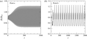
Reference Dionne, Ng and Lee2000; Sow, Chinnayya & Hadjadj Reference Sow, Chinnayya and Hadjadj2014). Figure 3 shows the period-one and period-two limit cycles arising from the instability of solutions at points a and b. The first bifurcation takes place at
 $D/D_{CJ}=0.986$
,
 $c_{f}=6.72\times 10^{-4}$
. In figure 3(a), a simple limit cycle is seen arising because of the presence of losses. Moving down along the top branch leads to a period-doubling bifurcation at
 $D/D_{CJ}=0.909$
,
 $c_{f}=4.57\times 10^{-3}$
. Figure 3(b) shows the evolution of
 $D$
starting at point b. We found that the period-two solution appears to continue down close to the turning point.
Detonation velocity as a function of time for solutions starting on the top branch of figure 1(a): (a) point a; (b) point b. The period of the limit cycle in (a) is
 $13.12$
.

To understand the stability properties of the set-valued solutions, we take point c on the top branch and point d in the set-valued region at the same value of
 $c_{f}$
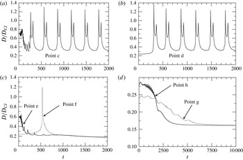
and calculate the detonation dynamics starting at these points. We find that the solution starting at c proceeds through a number of high-frequency oscillations up until
 $t\approx 100$
and then a rapid decay in velocity down to approximately
 $D/D_{CJ}=0.3$
–0.4 is seen with a subsequent initiation of large-amplitude low-frequency period-two oscillations around the point c, as shown in figure 4(a). Figure 4(b) displays a qualitatively different behaviour at early times – very slow increase of velocity with no oscillations. At approximately
 $t=300$
, we observe that the solution transitions to the same limit cycle as in figure 4(a), indicating that the trajectory is attracted to the top branch. The long-time behaviour of solutions starting at points c and d as well as other points in the set-valued region at the same
 $c_{f}$
are found to be identical. A different solution starting at the same
 $c_{f}$
, but closer to the boundary of the set-valued region is seen to transition to the top branch faster than the solutions starting from further down at lower velocities. What is common to all the solutions in the set-valued region is the presence of a non-oscillatory nearly steady early phase. The duration of this phase depends on the position in the set-valued region as well as on other factors, such as the activation energy.
Stability of the steady-state solutions at points c–h of figure 1(a).

Next, we look at the stability of the set-valued solutions at such
 $c_{f}$
that there is either no corresponding top branch or for which the top branch is near the turning point. The results are shown in figure 4(c–d). They are unstable again in both cases, but in figure 4(c), we see that both points e and f lead to detonation failure, even though the precise path is quite different in these cases. The set-valued point f leads to a long nearly steady solution that evolves to an explosion at approximately
 $t=500$
with a subsequent failure of the wave. Note that at this point, the transition to the upper branch toward point e takes place over a large set-valued region above f. Although the wave speeds up at the beginning as if attempting to make the transition, because of the proximity of the upper-branch solution to the turning point, the solution is strongly unstable resulting in the detonation failure.
Now we look at the points g and h for which there is no corresponding top branch (figure 4
d). In both cases, detonation fails. However, note that the decay is very slow initially, the wave remaining near its initial velocity for approximately
 $t=1500$
–2000. The sharp oscillations seen for point h early on are the consequence of local explosions overtaking the lead shock, which are similar to those observed at the transition in figure 4(a). Their extremely sharp appearance in figure 4(d) is due to the long scales of the time axis.
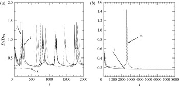
Stability of the steady-state solutions at points i–m of figure 1(b).

Figure 5 displays similar results for a larger activation energy,
 $E=27$
; all other parameters remain the same as before. In figure 5(a), case k, the solution appears to be essentially steady until
 $t\approx 600$
, at which point we see a rapid transition to the top branch. The dynamics of the solutions starting at j is similar to that starting at k, but with a shorter nearly steady stage. Comparison with the lower activation energy case indicates that increasing the activation energy leads to a more extended in time initial dynamics. Figure 5(b) demonstrates a behaviour similar to that at the lower activation energy of figure 4(c), but with a much more extended early transient stage, now continuing to approximately
 $t=2500$
.
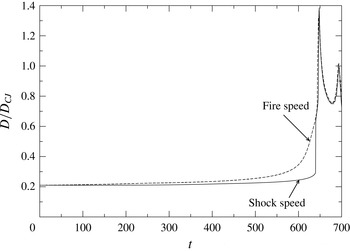
In figure 6, we show the velocities of the lead shock and the deflagration wave for the case of point k shown in figure 5(a). The two velocities appear to essentially coincide. The deflagration speed slightly exceeds the shock speed up until approximately
 $t=500{-}600$
. Then, the deflagration wave is seen to rapidly accelerate, forcing the lead shock to quickly transition to the top branch. After the transition, both fronts become closely coupled, with a much smaller distance between them than before the transition, and with similar velocities.
Low-velocity detonation at point k of figure 1(b) and its transition to the top branch. The speeds of the detonation and the deflagration waves as a function of time are shown.

5 The transition process
Here, we describe in some detail the process of the transition from the low-velocity to the high-velocity branch. The cases of successful transition (at
 $D/D_{CJ}=0.3$
, which is in the set-valued region just above point d in figure 1) and failure (point g) are considered. To elucidate the role played by different physical processes in the mechanism of the transition, we analyse various terms in the pressure evolution equation (written in the shock-attached frame)
 $$\begin{eqnarray}p_{t}=\underbrace{(D-u)p_{x}}_{1}\,\underbrace{-\unicode[STIX]{x1D6FE}pu_{x}}_{2}+\underbrace{(\unicode[STIX]{x1D6FE}-1)Q\unicode[STIX]{x1D70C}\unicode[STIX]{x1D714}}_{3}+\underbrace{(\unicode[STIX]{x1D6FE}-1)\frac{uf}{\unicode[STIX]{x1D719}}}_{4}\quad \underbrace{-(\unicode[STIX]{x1D6FE}-1)\frac{h}{\unicode[STIX]{x1D719}}}_{5}.\end{eqnarray}$$
This equation can be easily derived from the governing system (2.1). In the steady state, all the terms on the right-hand side of (5.1) balance to yield
 $p_{t}=0$
. Breaking of this balance leads to the local pressure change. The mechanism of the shock acceleration from the slow early regime to the fast pulsating long-term regimes is controlled by how different terms in (5.1) evolve in time and space. These terms have transparent physical meaning: (1)
 $(D-u)p_{x}$
is the rate of pressure rise due to the advection of nearby gas to the given location; (2)
 $-\unicode[STIX]{x1D6FE}pu_{x}$
is due to the compressibility of the gas; (3)
 $(\unicode[STIX]{x1D6FE}-1)Q\unicode[STIX]{x1D70C}\unicode[STIX]{x1D714}$
is due to the chemical heat release; (4)
 $(\unicode[STIX]{x1D6FE}-1)uf/\unicode[STIX]{x1D719}$
is the contribution by friction; and (5)
 $-(\unicode[STIX]{x1D6FE}-1)h/\unicode[STIX]{x1D719}$
is due to the heat loss.
We now focus on a successful transition that starts at a set-valued solution at
 $D/D_{CJ}=0.3$
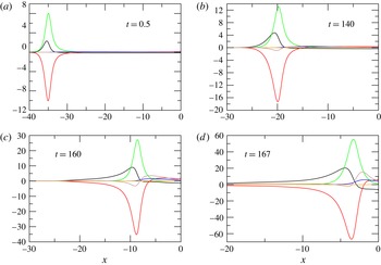
, a case chosen for its relatively low computational cost. We investigate the behaviour of all the terms in (5.1) at four different times from the beginning of the simulation as displayed in figure 7. What is notable in this figure is that the dominant effects in the fire (by which we refer to the chemical heat release profile) are those of advection (1), dilatation (2) and heat release (3). At
 $t=0.5$
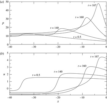
, an essentially steady-state structure is seen wherein the positive contributions due to the heat release and advection are balanced by the negative contribution due to the gas expansion. From approximately the middle of the fire downstream, the advection term is positive because
 $D-u>0$
and
 $p_{x}>0$
(see figure 8), i.e. the high-pressure gas from the front side of the fire is advected to the low-pressure region at the back. The dilatation term is negative there because of
 $u_{x}>0$
.
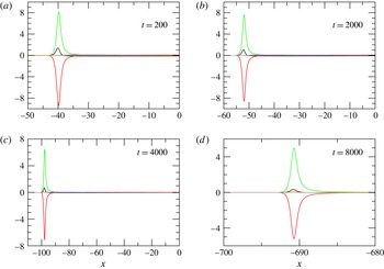
Contributions of different terms in the pressure equation (5.1) in the successful transition scenario at
 $D/D_{CJ}=0.3$
: (1) black; (2) red; (3) green; (4) blue; (5) orange; sum of all the terms - brown. The parameters are:
 $E=25$
,
 $Q=50$
,
 $\unicode[STIX]{x1D6FE}=1.2$
and
 $c_{f}=0.012$
. The computational domain size and resolution are
 $L=1000$
and
 $N_{1/2}=100$
, respectively.

Pressure (a) and velocity (b) profiles at different times corresponding to figure 7.

As time evolves, we observe that even though the same three effects remain dominant, some prominent changes to the profiles can be seen. Most interestingly, the chemical heat release profile advances upstream relative to that of the dilatation, that is, the expansion wave begins to lag behind the fire. As a result of this imbalance, a pressure build-up takes place in the fire region. The advective term (1) increases then on the back side of the fire, contributing more to balancing the expansion term than the heat release – see figure 7(c,d). The gas expands locally leading to the pressure drop, but that pressure drop is compensated by its rise due to the high-pressure gas advecting from the fire region. Ahead of the fire, the dilatation term is seen to begin to rise to large positive values, indicating that the gas is getting compressed there. This is a consequence of the pressure waves propagating toward the shock from the fire region. The friction term is seen to increase between the shock and the front side of the fire. Its contribution is now comparable to that of the compression. The advection term becomes negative in this region due to the change of the sign of the pressure gradient. Overall, on the front side of the fire, the heat release, friction and compressibility all contribute positively to the pressure rise, and dominate over the negative contribution of the advection term. The fastest growth of pressure is seen to take place at the front side of the fire where the friction effect is most significant. On the back side of the fire, the pressure time derivative becomes negative due to the strong expansion, which the weakening heat release there and the pressure advection are unable to compensate.
To summarize, the successful transition is characterized by the dominant roles played by the heat release, pressure advection, compressibility and friction, and by the compression waves generated by the fire region that create favourable upstream conditions for the fire to move toward the shock relative to the expansion wave.
In the failing scenario shown in figure 9, it is still heat release, expansion and advection that are the dominant players, however the fire is unable to move upstream relative to the position of the expansion wave. The fire is swept downstream with diminishing magnitudes of all the effects that contribute to the pressure rise. There is no noticeable pressure increase ahead of the fire.
Lastly, we point out that the heat-loss term is seen to be negligible in the fire region compared to all the other terms in (5.1). The heat loss is however dominant downstream in the velocity relaxation zone and is crucial due to its importance in establishing the steady-state equilibrium for the low-velocity solutions. Without the heat loss, there would be no set-valued steady state solutions, hence no slow transient evolution at the early times in the transition seen in figure 4(b).
Contributions of different terms in the pressure equation (5.1) in the failing scenario (point g): (1) black; (2) red; (3) green; (4) blue; (5) orange; sum of all the terms - brown. The parameters are:
 $E=25$
,
 $Q=50$
,
 $\unicode[STIX]{x1D6FE}=1.2$
and
 $c_{f}=0.012$
. The computational domain size and resolution are
 $L=1000$
and
 $N_{1/2}=100$
, respectively.

6 Discussion and conclusions
In this work, we analyse the stability properties of the set-valued solutions for gaseous detonations in systems with losses of momentum and heat. The peculiar nature of the steady-state solutions identified in Semenko et al. (Reference Semenko, Faria, Kasimov and Ermolaev2016) indicates that low-velocity one-dimensional detonations may be able to propagate in a nearly steady manner over long distances before transitioning to high-velocity regimes, predictions that we confirmed by the calculations made here. Thus, the existence of set-valued solutions points to a possible stabilization mechanism for low-velocity detonations observed in experiments. We find that solutions at low velocities are neutrally stable because they are not isolated. Any particular steady-state solution is surrounded by a continuum of other steady-state solutions. Therefore, perturbations of such solutions do not lead to strong instability, but rather lead to a slow continuous passage of the solution through the steady states in the set-valued region. For this reason, transition to the high-velocity regimes or failure of the wave are observed to take place over long time periods, during which the waves evolve in a nearly steady non-oscillatory fashion.
The early transients for the set-valued solutions which appear nearly steady have evolution time scales that are comparable to the particle passage times across the reactions zone of the corresponding steady-state solutions. Those time scales are much larger than the time scales of the ideal detonations at the same mixture parameters. The latter are the scales that are used in our computations. Thus, even though the early transients appear quasi-steady on the chosen
 $O(1)$
time scale of the ideal detonation, they are not quasi-steady on the time scale of the corresponding non-ideal solution. For this reason, we do not use the term ‘quasi-steady’ in referring to these solutions. Nevertheless, the ideal time scales are the appropriate reference scale for all the solutions, and the low-velocity waves do indeed appear nearly steady on those scales. One could draw a parallel with an actual physical experiment in which the velocities of the LVD are compared with the ideal velocities with both measured on the same time scale.
The existence of the large set of solutions at low velocities implies a certain degree of indeterminacy – there appears to be no simple mechanism that selects a particular solution in the set-valued region. In other words, nearly steady regimes in a wide range of velocities are possible depending on particular initial conditions. As explained in Semenko et al. (Reference Semenko, Faria, Kasimov and Ermolaev2016), the existence of the set-valued solutions is tied to the indeterminacy of the boundary conditions at infinity. Once the temperature or pressure at infinity is specified, a particular
 $D$
–
 $c_{f}$
curve is selected from the infinite set. Therefore, the choice of a particular solution for the low-velocity detonation depends on the conditions far downstream.
The previous discussion is consistent with the experimental observations, which have shown that waves propagating in a continuous range of velocities between the ambient sound speed and the ideal velocity are often observed (Lyamin et al.
Reference Lyamin, Mitrofanov, Pinaev and Subbotin1991). Our simulations indicate similar behaviour: nearly steady solutions exist at all velocities within the set-valued range that correspond to the sonic-velocity regimes or the low-velocity detonation regimes. At the lower end of the velocity range, frictional heating of the gas is responsible for sustaining the reaction. As the velocity increases, so does the role of shock heating relative to frictional heating. On the upper branch of the
 $D$
–
 $c_{f}$
curve, above the set-valued region (i.e. in the ‘quasi-detonation’ regime), the shock heating is dominant. These conclusions are consistent with several existing proposals on the mechanisms of such detonations (Babkin et al.
Reference Babkin, Korzhavin and Bunev1991; Korzhavin et al.
Reference Korzhavin, Bunev, Babkin, Lawes and Bradley1999; Babkin Reference Babkin2012).
Our present findings suggest a stabilization mechanism to the unconditionally unstable behaviour of solutions near the middle branch of a typical reverse
 $S$
shaped response curve that is found in the absence of heat losses. The presence of heat losses is then a key to this mechanism, as no set-valued solutions exist without heat losses. We should emphasize that the low-velocity regimes we computed here are not steady-state stable solutions. They are nearly steady long-lived neutrally stable regimes that eventually fail or transition to high-velocity regimes.
All the preceding conclusions apply to smaller activation energies as well. We observe qualitatively the same dynamics. At large activation energies, we find that detonation often fails, even when starting the solution on the top branch. We remark finally that in view of the simplified nature of the modelling employed here as far as the reaction rate and loss factors, our predictions are primarily qualitative in nature. It is therefore important to investigate how these predictions can be extended and compared with available experiments at a quantitative level. Our preliminary calculations indicate that for the quantitative agreement, modifications are necessary as to the specific forms of the heat release function, loss terms and mixture thermodynamics (Kasimov & Semenko Reference Kasimov and Semenko2016). However, the one-dimensional modelling with more complex physics still yields set-valued solutions, and the computed
 $D$
–
 $c_{f}$
dependencies are found to be closer to experimental data with an appropriate choice of the modelling parameters. We intend to continue our exploration of the underlying mechanisms of low-velocity solutions with such complex modelling and hope to report our findings in a follow-up work.
Acknowledgements
Research reported in this publication was supported by the King Abdullah University of Science and Technology (KAUST).