Introduction
The Class Cephalopoda of the Phylum Mollusca includes octopus, cuttlefish, squid, and the nautilus. Due to the high consumption rate and overfishing of finfish, cephalopods have been considered an alternative protein source in the human diet (Jereb et al., Reference Jereb, Roper, Norman and Finn2014). Cephalopod fisheries are classified according to the mechanism of capture and volume of catch, and are defined as large-scale (e.g. jig fishing), by-catch (e.g. bottom trawling, lobsters traps, hook and line), and small-scale (e.g. pots, fishing by hand, hook) (Rodhouse et al., Reference Rodhouse, Pierce, Nichols, Sauer, Arkhipkin, Laptikhovsky, Lipiński, Ramos, Gras, Kidokoro, Sadayasu, Pereira, Lefkaditou, Pita, Gasalla, Haimovici, Sakai, Downey and EAG2014; Sauer et al., Reference Sauer, Gleadall, Downey-Breedt, Doubleday, Gillespie, Haimovici, Ibáñez, Katugin, Leporati, Lipinski, Markaida, Ramos, Rosa, Villanueva, Arguelles, Briceño, Carrasco, Che, Chen and Yamrungrueng2019). In the past 20 years, the number of cephalopods caught has increased, with a peak of 4.9 million tonnes reported in 2014 (FAO, 2020). Most of these catches belong to four distinct cephalopod families, Loliginidae, Ommatrephidae, Octopodidae, and Sepiidae (Sauer et al., Reference Sauer, Gleadall, Downey-Breedt, Doubleday, Gillespie, Haimovici, Ibáñez, Katugin, Leporati, Lipinski, Markaida, Ramos, Rosa, Villanueva, Arguelles, Briceño, Carrasco, Che, Chen and Yamrungrueng2019; Ospina-Alvarez et al., Reference Ospina-Alvarez, De Juan, Pita, Ainsworth, Matos, Pita and Villasante2022).
The highest numbers of octopus landings in the Caribbean are reported in Mexico and Venezuela (Sauer et al., Reference Sauer, Gleadall, Downey-Breedt, Doubleday, Gillespie, Haimovici, Ibáñez, Katugin, Leporati, Lipinski, Markaida, Ramos, Rosa, Villanueva, Arguelles, Briceño, Carrasco, Che, Chen and Yamrungrueng2019). These regions have several cephalopod species of commercial interest, including Octopus vulgaris Cuvier, 1797. However, most countries do not identify octopus catches by species; therefore, the importance of O. vulgaris in the market is unknown (Lourenço, Reference Lourenço2014). In Puerto Rico, annual catches range from 5000 to 18,000 kg, with the south coast reporting the highest number of catches (Figure 1). Although there is no separation by species in landing reports, O. vulgaris is commonly considered the most abundant octopus in Puerto Rico.
Reported landings of Octopus spp. by artisanal fishers in Puerto Rico from 2012 to 2017 and 2019 to 2021 (uncorrected data). Hurricane Maria significantly impacted the artisanal fishers in September 2017, which may have caused some bias in the data for this year. Landings from 2018 and region data from 2019 to 2021 were not provided. Daniel Matos and Martha Ricaurte provided the data from the Fisheries Research Laboratory of the Department of Natural and Environmental Resources of Puerto Rico (DNER-PR).

Octopus vulgaris is a merobenthic organism and is considered a species with a worldwide distribution (Amor et al., Reference Amor, Norman, Roura, Leite, Gleadall, Reid, Perales-Raya, Lu, Silvey, Vidal, Hochberg, Zheng and Strugnell2017). However, studies in phylogeny and population structure suggest that octopuses treated as O. vulgaris are paraphyletic, suggesting the presence of a ‘cryptic species complex’ composed of morphologically similar but genetically distinct species (Söller, Reference Söller2000; Amor et al., Reference Amor, Norman, Cameron and Strugnell2014). Amor et al. (Reference Amor, Doyle, Norman, Roura, Hall, Robinson, Leite and Strugnell2019) used nuclear DNA and the double-digest restriction-site associated DNA sequencing (ddRADseq) protocol (Peterson et al., Reference Peterson, Weber, Kay, Fisher and Hoekstra2012) to estimate the phylogenetic relationships within this species complex; at the locations sampled, they found six species within the O. vulgaris complex. According to their suggestions, the species within this complex seem to be separated geographically into different regions. Octopus vulgaris species type I is present in the Caribbean and Gulf of Mexico regions. Species type II is present in southern Brazil, while species type III is present in South Africa. Octopus tetricus is present in eastern Australia, and Octopus cf. tetricus is present in western Australia. Octopus sinensis is found in Asia, while O. vulgaris sensu stricto is found in the Mediterranean and eastern North Atlantic regions (Amor et al., Reference Amor, Doyle, Norman, Roura, Hall, Robinson, Leite and Strugnell2019). They also observed that the ddRADseq approach provides higher resolution than traditional markers, such as mitochondrial markers, used in other phylogenetic studies of the O. vulgaris species complex.
Because high dispersal is often expected in organisms that live in the sea where no obvious physical barriers exist, marine organisms should present high levels of genetic connectivity – the exchange of individuals within the same species during any stage in their lives (Palumbi, Reference Palumbi2003) within populations and low levels among populations (Fadhlaoui-Zid et al., Reference Fadhlaoui-Zid, Knittweis, Aurelle, Nafkha, Ezzeddine, Fiorentino, Ghmati, Ceriola, Jarboui and Maltagliati2012). However, there are apparent barriers (e.g. currents, water bodies with temperature differentials, vast areas of unsuitable habitats, and diverse means of dispersal), resulting in a realized dispersal that may be different than the one inferred from the potential dispersal based on life strategies. In benthic marine organisms, the potential of genetic connectivity is limited after the settlement phase of the individual (Cowen and Sponaugle, Reference Cowen and Sponaugle2009).
Octopus vulgaris is characterized by having semelparity as a reproductive strategy (Rocha et al., Reference Rocha, Guerra and González2001). After hatching, its first stage of life is known as paralarvae, which measures 2–3 mm (Jereb et al., Reference Jereb, Allcock, Lefkaditou, Piatkowski, Hastie, Pierce, Jereb, Allcock, Lefkaditou, Piatkowski, Hastie and Pierce2015). This planktonic period depends on the temperature and the diet to which the paralarvae are exposed. Laboratory studies using temperatures of 19–26.7°C found that the paralarvae phase lasts for 30–60 days (Iglesias et al., Reference Iglesias, Sánchez, Bersano, Carrasco, Dhont, Fuentes, Linares, Muñoz, Okumura, Roo, Meeren, Vidal and Villanueva2007; Morales et al., Reference Morales, Cardenete, Hidalgo, Garrido, Martín and Almansa2017). After this phase, O. vulgaris settles on the seafloor to begin its benthic life. As adults, during the reproductive stage, male O. vulgaris can reproduce multiple times, while females reproduce only once in their lives and can store sperm from different males (Silva et al., Reference Silva, Sobrino and Ramos2002). In a study conducted at Nueva Esparta, Venezuela, the minimum size and weight registered for sexual maturity in males were 11 cm and 428 g, respectively, while the minimum size and weight for females were 12 cm and 476 g (González et al., Reference González, Eslava, Guevara and Troccoli2015).
Previous molecular studies of O. vulgaris have primarily used 16S ribosomal ribonucleic acid, cytochrome oxidase I, cytochrome oxidase III, cytochrome b, and different microsatellites (Jassoud, Reference Jassoud2010; De Luca et al., Reference De Luca, Catanese, Procaccini and Fiorito2014). In the last decade, scientists have used either single markers or a combination of several molecular markers to measure the genetic connectivity of O. vulgaris in different parts of the world. Some have shown significant genetic differences using microsatellites or a single molecular marker (Moreira et al., Reference Moreira, Tomás and Hilsdorf2011; Beer, Reference Beer2014; Melis et al., Reference Melis, Vacca, Cuccu, Mereu, Cau, Cristina and Rita2018; Van Nieuwenhove et al., Reference Van Nieuwenhove, Ratsimbazafy and Kochzius2019). Although the studies using mitochondrial genes and microsatellites provide a perspective of genetic connectivity, they can be conservative, and each method can lead to different results (Oosthuizen et al., Reference Oosthuizen, Jiwaji and Shaw2004; De Luca et al., Reference De Luca, Catanese, Procaccini and Fiorito2014). Massively-parallel, short read sequencing techniques such as restriction-site associated DNA sequencing (RADseq) have become popular in population genomics as they allow the study of more areas of the genome to obtain high-resolution molecular information (Sotil and Cueva, Reference Sotil and Cueva2019). For example, Pfaller et al. (Reference Pfaller, Mcdaniel, Payton, Bjorndal and Bolten2019) used RADseq and traditional mitochondrial DNA sequencing in Planes crabs; they observed that genome-wide markers such as RADseq allow for identifying patterns of population structure in organisms that show high connectivity over long distances, contrasting a more conservative analysis obtained from a single gene. To understand the population dynamics of three deep-sea cephalopod species in the Gulf of Mexico and the Atlantic, researchers analysed ddRADseq (a variant of RADseq) and traditional Sanger sequencing methods. They found high diversity in all species, with population structure in one species and the other two species comprising a single population (Timm et al., Reference Timm, Bracken-Grissom, Sosnowski, Breitbart, Vecchione and Judkins2020). The aforementioned studies and others showcased how advances in sequencing technology allowed for the development of more efficient and cost-effective molecular techniques with great power to make inferences in genetic population studies. Many of these studies suggest that despite the absence of physical barriers (e.g. a land mass), differential oceanographic characteristics (e.g. currents with different physico-chemical properties) can function as biogeographic barriers, preventing larval exchange.
Our study aims to investigate the genetic diversity and connectivity of O. vulgaris in the Puerto Rico Archipelago. To achieve this, we employed the ddRADseq protocol, using the restriction enzymes EcoRI and SphI. We followed a reference genome-based protocol to align the sequences against the published O. vulgaris reference genome assembly (accession GCA_951406725.2), from which we can genotype individuals for multiple, independent single-nucleotide polymorphisms (SNPs) (Catchen et al., Reference Catchen, Hohenlohe, Bassham, Amores and Cresko2013; Destanović et al., Reference Destanović, Schultz, Styfhals, Cruz, Gómez-Garrido, Gut, Gut, Fiorito, Simakov, Alioto, Ponte and Seuntjens2023). We hypothesized that the geographic distance between regions and oceanographic conditions surrounding Puerto Rico, such as east-northeast trade winds, eddies, the Mona Passage water inflow, and the seasonal Orinoco and Amazon freshwater plums, would likely lead to a detectable degree of genetic structure (Wüst, Reference Wüst1964; Gordon, Reference Gordon1967; Richardson, Reference Richardson2005; Chérubin and Richardson, Reference Chérubin and Richardson2007). By applying molecular techniques, we can gain insights into marine organisms' genetic diversity and population structure. These parameters can be useful to evaluate the effectiveness and limitations of existing marine protected areas (MPAs) and generate new MPAs that operate as a network to preserve species diversity (Jenkins and Stevens, Reference Jenkins and Stevens2018). These genetic data can support stakeholders in enhancing the design of MPAs and making science-based decisions for the sustainable management of fisheries in Puerto Rico.
Materials and methods
Sample collection and handling procedure
We collected 54 octopus tissue samples from ten locations between October 2020 and October 2021. Based on gel electrophoresis results, we discarded 11 samples due to poor DNA quality. In total, 43 samples underwent DNA sequencing. These samples represent three regions in the Puerto Rico Archipelago: the north (Aguadilla n = 6, Arecibo n = 4, Camuy n = 5, and San Juan n = 1), south (Cabo Rojo n = 4, Lajas n = 4, Penuelas n = 6, and Guayama n = 5), and east (Fajardo n = 5 and Vieques n = 3) regions (Figure 2). The samples were collected while snorkeling with the aid of local fishers. We have the coordinates of the sites; however, we will not reveal them as a sign of respect to the fishers who helped in this work. The fishers kept the octopus, and we collected the tip of one of the arms of each octopus, approximately 3–6 cm long. At the time of collection, the samples were stored in 95% ethanol and kept on ice. Subsequently, they were frozen at −80°C for downstream genetic analysis.
Map of Puerto Rico with sampling sites (Google Earth Pro, 2024).

DNA extraction and molecular techniques
We used the QIAGEN DNeasy Tissue Kit protocol to extract genomic DNA. However, we modified the protocol in the following way: first, we added tissue lysis buffer (ATL) (180 μl) and proteinase K (25 μl) to the sample and gently shook the microtube without vortexing. We then incubated the sample for 12–15 h. If tissue was still visible in the microtube after this time, we added ATL buffer (100 μl) and proteinase K (15 μl) and incubated it for 3–5 h until the tissue was dissolved. As a quality measurement, we performed electrophoresis on a 0.7% agarose gel in 1 × TBE buffer to assess DNA quality, and as a second quality measurement, we estimated DNA concentration using a Qubit 4.0 Fluorometer. Then, we sent samples with high-quality DNA showing a bright high-molecular weight band in the electrophoresis, and with concentrations over 10 ng μl−1 to the Admera Health genomic facility (New Jersey) for genomic library preparation and sequencing. We used a ddRADseq protocol using EcoRI and SphI restriction enzymes for genomic digestion (Peterson et al., Reference Peterson, Weber, Kay, Fisher and Hoekstra2012). The libraries were paired-end sequenced (2 × 150 bp) on an Illumina NovaSeq X plus 10B platform with the Illumina TruSeq adapter design (Supplementary Table S1). The samples were sequenced by multiplexing across two batches (refer to the Results section for further details).
Initial processing of raw sequences
We used the following software to clean, filter, and analyse the data: Stacks V2.65 (Rochette et al., Reference Rochette, Rivera-Colón and Catchen2019,) BWA V0.7.12 (Li and Durbin, Reference Li and Durbin2009), SAMtools V1.18 (Li et al., Reference Li, Handsaker, Wysoker, Fennell, Ruan, Homer, Marth, Abecasis and Durbin2009), and Structure V2.3.4 (Pritchard et al., Reference Pritchard, Stephens and Donnelly2000). First, we followed the Stacks manual to demultiplex (i.e. assign sequence reads to individuals) the raw data (Rochette et al., Reference Rochette, Rivera-Colón and Catchen2019; Rivera-Colón and Catchen, Reference Rivera-Colón, Catchen, Verde and Giordano2022). We ran process_radtags V2.65 in Stacks using the following commands: identifying the path to the raw data files (-P), indicating the path to the barcodes list (-b), cleaning the data (-c), removing low-quality reads (-q), identifying where is the barcode in the FASTQ file (--index-index), indicating the restrictions enzymes used (--renz-1 Sph1 --renz-2 ecoR1), followed by the adapters sequences (--adapter_1 and --adapter_2), and indicating 0 mismatches allowed when matching the adapter (--adapter_mm 0).
Reference alignment
After finishing the process_radtags run, we downloaded the Octopus vulgaris reference assembly (accession GCA_951406725.2) from the National Library of Medicine database in order to align the ddRADseq reads (Destanović et al., Reference Destanović, Schultz, Styfhals, Cruz, Gómez-Garrido, Gut, Gut, Fiorito, Simakov, Alioto, Ponte and Seuntjens2023). For this step, we used BWA and SAMtools following their corresponding manuals (Li et al., Reference Li, Handsaker, Wysoker, Fennell, Ruan, Homer, Marth, Abecasis and Durbin2009; Li and Durbin, Reference Li and Durbin2009). At this step, we had two files, one containing the forward and the other the reverse reads of each sample. First, we called BWA to index the genome (index), and then we aligned all the samples against the genome (mem) using the path to the reference genome and the samples directory. Finally, SAMtools were used to sort the samples by genomic coordinates (view and sort) and to produce one BAM file per sample containing both paired reads to use in Stacks for further analysis.
SNP discovering and variant calling
After alignment, we used the ref_map.pl V2.65 wrapper program in Stacks to assemble loci and genotype individuals. The ref_map.pl program runs gstacks, followed by the populations program. For this step, we followed the example from Rivera-Colón and Catchen (Reference Rivera-Colón, Catchen, Verde and Giordano2022), adjusting the parameters according to the behaviour of our data. First, we made a population map file (‘pop map’), in which we indicated the name of the samples and the assigned population. In this case, we had ten sampling locations divided into three regions (north, south, and east) used as populations in the ‘pop map’. Then, we provided the path to the samples (--samples), the path to the ‘pop map’ (--popmap), the filters for SNP discovering and for variants calling, respectively (-X ‘gstacks: --var_alpha 0.1’) and (-X ‘gstacks: --gt_alpha 0.01’), indicated the number of threads that we wanted to use (-t), and finally, the output directory (--out-path). After this step, we continued running the populations program, applying different filters, and using different samples per run. For populations, we indicated the input path (--in-path), the ‘pop map’ (--popmap), and the output path (--out-path). Then we used the following filters: considering the three regions (--min-populations 3), processing a locus that is at least in the 50% of individuals across populations (--min-samples-overall 0.50), minimum allele count of 3 to process an SNP (--min-mac 3), calculating differences for Hardy-Weinberg equilibrium for each locus (--hwe), selecting the first SNP per locus (--write-single-snp), computing F-statistics (--fstats), and producing an output text file (--structure) for further analysis using Structure software V2.3.4 (Pritchard et al., Reference Pritchard, Stephens and Donnelly2000).
Analysis of population structure
We analysed the output genotypes from Stacks for the genetic clustering analysis in Structure. We ran the pipeline in the command line, making several runs, using the Structure_theader wrapper program to parallelize and speed up the runs (Pina-Martins et al., Reference Pina-Martins, Silva, Fino and Paulo2017). Simulations were conducted until alpha achieved constant rate. These simulations varied in burning periods, Markov Chain Monte Carlo (MCMC) repetitions, K, and iteration counts. After evaluating the data, the last test was K = 1 to K = 10 with ten iterations, using a 30,000-burning period and 100,000 MCMC repetitions. The parameters that we changed in the ‘mainparams’ and ‘extraparams’ files were the location information ‘Popdata’, and the ‘Freqscore’ when testing the correlated allele frequency model (Falush et al., Reference Falush, Stephens and Pritchard2003). We used the following commands to perform the test: enabling logging run information to a file (--log), indicating the population numbers (-K), the input file (-i), the path to the Structure directory (-st), the numbers of threads (-t), and the path to the ‘mainparams’ and ‘extraparams’ files (--params).
After finishing the analysis, we evaluated the delta K calculated by Structure Harvester using the Evanno method and made plots from the results files using Structure_threader (Earl and vonHoldt, Reference Earl and vonHoldt2012; Pina-Martins et al., Reference Pina-Martins, Silva, Fino and Paulo2017). We performed two runs, one using a ‘popfile’ to group the samples by region and the other using an ‘Indfile’ to process the samples individually. We used the following commands (-i, -st, -o, -K) and added the (--popfile) and (--indfile) in separate runs.
As a second approach to analyse how different individuals cluster into groups and the distance between them, we performed a principal components analysis (PCA). To perform the PCA, we used the Adegenet V2.1.10 package (Jombart, Reference Jombart2008) in Rstudio V4.3.0 (R Core Team, 2023; RStudio Team, 2020). We followed the following steps: we created a ‘genind object’ of the Structure output file from Stacks (read.structure), created an allele frequency table (tab), indicated that missing values will be replaced the mean allele frequency at each marker (na.method = ‘mean’), we retained three axes (nf = 3) and calculated the PCA (dudi.pca). Finally, we make a plot using the principal components (PC1 and PC2) on the assigned populations (s.class).
For the statistical analysis, we used Arlequin V3.5.2.2 software (Excoffier and Lischer, Reference Excoffier and Lischer2010). First, we used GPDSpider V2.1.1.5 software to convert the Structure file into Arlequin format (Lischer and Excoffier, Reference Lischer and Excoffier2012). In Arlequin, we configured the project settings using the three populations (north, south, and west). Second, we performed a standard and a locus-by-locus analysis of molecular variance (AMOVA) using 20,000 permutations, to get a broad picture and examined each locus contribution to the genetic variation (Excoffier et al., Reference Excoffier, Smouse and Quattro1992; Wares et al., Reference Wares, Alò and Turner2004). We performed a pairwise F ST test using 20,000 permutations with a significance level of 0.05%, also we conducted a nucleotide diversity (π) test, and a standard genetic diversity indices test.
Results
Quality control and processing of raw data
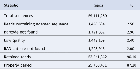
We received 59,111,280 sequence reads from the 43 samples from the sequencing centre (Table 1) (accession PRJNA1167657). First, we used the process_radtags program to filter the data. The results showed that there were 1,496,534 (2.5%) reads containing adapter sequences and that the barcodes were not found in 1,721,332 (2.9%) of the reads. We also removed, 1,443,109 (2.4%) of low-quality reads, and 1,208,943 (2.0%) of the reads where the RAD cut site was not found. In total, we retained 53,241,362 (90.1%) of the reads and, on average, 91.45% read-pairs per sample. Secondly, after aligning the samples with the Octopus vulgaris reference genome, 25,758,411 (87.2%) were properly paired. When analysing the retained reads per sample, we decided to remove the sample OV_GUA4 from the analysis, as we detected an error of three erroneous, extra nucleotides in the barcode resulting in 0% of pair reads retained.
Summary statistics after applying the process_radtags command in the program Stacks

Assembly of loci and genotype filtering
After applying the filters of the ref_map.pl program to the 42 remaining samples, gstacks kept 19,478,197 (37.8%) primary alignments, with a total of 25.2–36.1% reads kept per sample. The program built 70,579 loci comprising 6,198,600 matching read pairs. The mean depth of coverage per sample was 23.5x, with a standard deviation of 13.2x, and minimum and maximum per-sample coverages of 7.3x and 52.5x, respectively. The assembled loci were 198.7 sites long, on average. A total of 28,369 of 31,316 (90.6%) loci with multiple SNPs were reliably phased.
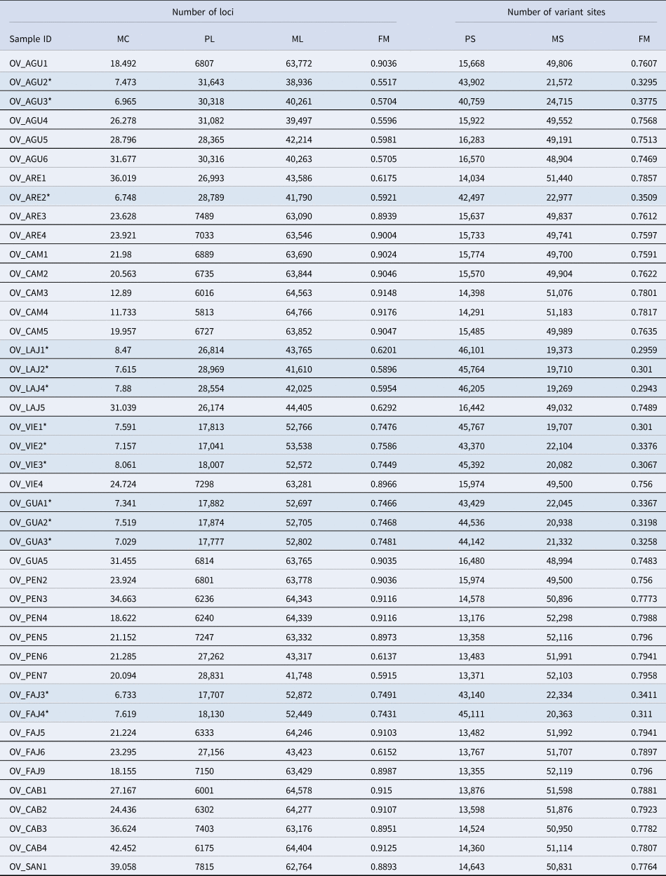
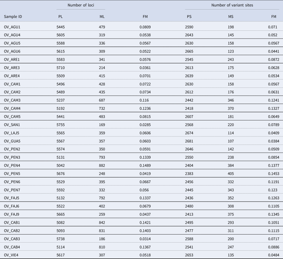
Subsequently, we ran the populations program to apply missing-data filters, and kept 12,457 out of the 70,579 assembled loci. The retained loci comprised of 2,988,573 sites, of which 3153 were variant sites. The mean genotyped sites per locus was 78.52 bp. After analysing the missing data and coverage statistics, we noticed that the dataset split into two groups. One group of 14 samples retained more loci than the other group of 29 samples (Table 2). The 14 samples retaining more loci had <10x of coverage and more missing variant sites than the other 29 samples. Following the guidelines described in Rivera-Colón and Catchen, (Reference Rivera-Colón, Catchen, Verde and Giordano2022), we decided to remove the 14 samples with more missing variant sites and continue the analysis with the remaining 29 samples. To achieve this, we made a new population map comprised of 29 samples (Table 3). After filtering, we kept 5924 loci composed of 1,113,304 sites, of which 2788 were variant sites. The mean genotyped sites per locus was 163.68 bp. For statistics of the ‘pop map’ comprising the removed batch (14 samples), refer to Supplementary Tables S2 and S3. It is important to note that after the filtering process, four localities (San Juan, Lajas, Guayama, and Vieques) were represented by only one sample (refer to the Discussion section for further details).
Mean coverage, number of loci, and variant sites per sample after applying ref_map.pl program filters in the program Stacks

MC, mean coverage; PL, present loci; ML, missing loci; FM, frequency missing; PS, present site; MS, missing site.
The samples in grey with the * were removed from the analysis.
Number of loci and variant sites per sample after running the Stacks populations program on the 29 kept samples

PL, present loci; ML, missing loci; FM, frequency missing; PS, present site; MS, missing site.
Clustering analysis
First, we analysed results from Evanno's ΔK test based on Structure analysis. The highest delta K (3.02) indicates that K = 4 is the best K for our dataset (Supplementary Figure S1), meaning that our samples can be allocated among four genetic clusters. However, in all the samples, one of the clusters dominated with at least 40% of the assignment (Figure 3). Most of the north region samples are represented between clusters one and two; with the exceptions of OV_CAM1 (cluster three), OV_CAM5, and OV_SAN1 (cluster zero). The south region was dominated by clusters three, one, and zero. The east region was represented in clusters zero, two, and three. As in the Structure clustering analysis, the PCA result represents a mixed scenario with no evidence of differentiation, as defined by overlap between the samples from different geographic regions (Figure 4).
Structure clustering results of K = 2 to K = 4 using the correlated allele frequency model. Each bar represents an individual octopus, and the black line divisions represent the regions. The colours represent the assigned cluster proportion per individual.

PCA representing the 29 octopus samples divided into north, east, and south. PC1 explains 14.91% and PC2 14.49% of variation.

Genetic diversity and structure analysis
We used loci with <10% of missing information for the statistical analysis in Arlequin. In the north region, we used 951 SNPs found in 2160 loci; in the south, 922 SNPs from 2152 loci; and in the east, 648 SNPs were identified in 2119 loci. The observed heterozygosity (H O) and expected heterozygosity (H E) were 0.256 and 0.258 in the north region, with a nucleotide diversity (π) of 0.110. The south region presents an H O and H E of 0.255 and 0.261 with a π of 0.109. The east region expressed an H O and H E of 0.361 and 0.373 with a π of 0.114.
In summary, all the regions presented an average nucleotide diversity (π) of 0.1 and similar levels of heterozygosity. The pairwise distance computations between east and south were 0.001, between east and north 0.005, and between north and south 0, indicating a small genetic distance between these geographic regions. We used 1988 loci to compute the standard AMOVA and inbreeding coefficients with a significance level of 0.01. Results did not indicate a significant genetic structure and attributed 99.69% of the variance within individuals (Table 4). No significant evidence of inbreeding was found (F IS = 0.002 and F IT = 0.003). We also found no significant relative genetic differentiation (F ST) between the different regions, between east and south (P-value = 0.444), between north and south (P-value = 0.579), and between east and north (0.151). However, in the locus-by-locus AMOVA, the inbreeding coefficients (F IS = 0.060 and F IT = 0.064) were significant (Table 5), indicating more homozygotes than expected and a deviation from random mating.
Standard AMOVA and fixation indices using 1988 loci

Locus-by-locus AMOVA and fixation indices using over 1303 polymorphic loci

The significant values are represented in bold and with *.
Discussion
Overview
Biological and physical factors play a crucial role in the larval and adult exchange of marine populations (Álvarez-Noriega et al., Reference Álvarez-Noriega, Burgess, Byers, Pringle, Wares and Marshall2020). It is vital to incorporate interdisciplinary data sets to gain a more comprehensive understanding of realized dispersal processes, especially when we are studying commercially important species. In this context, conservation genomics is a field that can provide essential information to scientists and resource managers alike. RADseq approaches have become more common in population genomics research, leading to valuable discoveries (Andrews et al., Reference Andrews, Good, Miller, Luikart and Hohenlohe2016). For example, these approaches have been used for the reintroduction and genetic management of Burmese roof turtles (Çilingir et al., Reference Çilingir, Rheindt, Garg, Platt, Platt and Bickford2017), studying the spatial patterns and population dynamics of Nassau grouper (Sherman et al., Reference Sherman, Paris, King, Moore, Dahlgren, Knowles, Stump, Tyler and Stevens2020), and identifying patterns of dispersal of sea scallop Placopecten magellanicus (Van Wyngaarden et al., Reference Van Wyngaarden, Snelgrove, DiBacco, Hamilton, Rodríguez-Ezpeleta, Jeffery, Stanley and Bradbury2017). Here, we present the first small-scale genetic study that assesses the connectivity and diversity of Octopus vulgaris in Puerto Rico using a ddRADseq approach. Using SNP data, this study represents a significant step forward in understanding O. vulgaris genetics and its implications for the Western-Central Atlantic region.
Clustering analysis
After applying the Evanno method (Supplementary Figure S1 and Table S4), the cluster analysis conducted in Structure for k = 4 suggested four genetic clusters. The proportion of clusters per individual is variable, and there is no correlation between the assigned geographic regions and cluster assignment (Figure 3). Except for Aguadilla, where one of the clusters is dominant, there is no evidence of individuals grouping in clusters according to their sampling locations. While cluster two predominantly comprises north region individuals, there is no clear indication that the other clusters exhibit regional grouping. The PCA plot (Figure 4) shows no evidence of sample clustering based on region. Most individuals are grouped, suggesting a lack of differentiation among regions. Based on the results obtained from the PCA and F-statistics analyses, there is no evidence to support the existence of four distinct, and spatially delimited genetic groups, as suggested by Structure. Instead, it is more likely that all individuals are admixed, and the model indicates the variation shared by each individual (Lawson et al., Reference Lawson, Van Dorp and Falush2018).
Genetic diversity and connectivity
All the assayed geographic regions showed relatively high nucleotide diversity (π of 0.1), compared to low π reports using mitochondrial markers (Melis et al., Reference Melis, Vacca, Cuccu, Mereu, Cau, Cristina and Rita2018; Van Nieuwenhove et al., Reference Van Nieuwenhove, Ratsimbazafy and Kochzius2019). The heterozygosity (H E and H O) values were moderate, and differed from those shown in Cabranes et al. (Reference Cabranes, Fernandez-Rueda and Martínez2008) and De Luca et al. (Reference De Luca, Catanese, Procaccini and Fiorito2016), which reported high levels of heterozygosity in O. vulgaris populations in the Mediterranean Sea and the Canary Islands. The observed heterozygosity was almost equal to the expected value in all the regions, in contrast to the findings by De Luca et al. (Reference De Luca, Catanese, Procaccini and Fiorito2016), which suggests an excess of homozygosity. The standard and locus-by-locus AMOVA analysis presented a low F ST, indicating small relative differentiation and suggesting high connectivity between regions. The standard AMOVA did not show significant results for the inbreeding coefficients F IS (relationship of genes among individuals within subpopulations) and F IT (relationship of genes within individuals of the total population) (Weir and Cockerham, Reference Weir and Cockerham1984); however, F IS and F IT were significant when performing the locus-by-locus AMOVA (Table 5). When exploring this analysis, we detected that samples from the east region had fewer polymorphic loci presented in comparison to the other regions. This significant result in the locus-by-locus AMOVA could be attributed to the difference in individuals analysed in the east (N = 4) compared to the north (N = 13) and south (N = 12), which have more individuals and more polymorphic loci. If F IS and F IT had an unbiased significant result, we would expect a more considerable difference between H O and H E (De Luca et al., Reference De Luca, Catanese, Procaccini and Fiorito2016). It is important to mention that in Arlequin the locus-by-locus AMOVA test uses only the polymorphic loci, contrasting from the standard AMOVA that analyses polymorphic and not polymorphic loci; this could drive the difference presented in F ST (0.005 and 0.0008).
Oceanographic characteristics are variable and differ yearly; Ojeda (Reference Ojeda2002) suggests that larvae retention or dispersal potential on the southwest coast of Puerto Rico will depend on the oceanographic conditions presented at the hatching time. In this regard, Pagán (Reference Pagán2003) suggests that the westward flow (November to August) and a nearby eddy may promote the retention of larvae on the insular shelf. However, Xu (Reference Xu2022) found that the eastward flow facilitated the larval dispersal through the south and north coasts from the U.S. Virgin Islands (USVI) to Puerto Rico. Xu (Reference Xu2022) used drifters and a larval dispersal model to evaluate the larval retention of the snapper Lutjanus analis and the grouper Epinephelus guttatus spawning aggregations between the USVI and Puerto Rico. Although they only evaluated three spawning sites from December to February and June to July, our results align with their observations, suggesting high connectivity between the regions. Despite the different life cycles of O. vulgaris compared to L. analis and E. guttatus, they all have a planktonic stage driven by currents. Octopus vulgaris paralarvae can last 30–60 days in the water column, and female O. vulgaris can store sperm from different males, leading to multiple paternity, which influences genetic connectivity (Quinteiro et al., Reference Quinteiro, Baibai, Oukhattar, Soukri, Seixas and Rey-Méndez2011; Morales et al., Reference Morales, Cardenete, Hidalgo, Garrido, Martín and Almansa2017). The eastward flow described by Xu (Reference Xu2022) seems to help the dispersion of larvae along the south and north coasts of Puerto Rico, promoting connectivity between regions and allowing paralarvae to spread across wider geographic areas. Despite the localized oceanographic features, such as the westward flow and nearby eddies, which may promote larval retention (Ojeda, Reference Ojeda2002; Pagán, Reference Pagán2003), this broader eastward flow appears to override localized retention effects.
Our results differ from previous large-scale and small-scale studies using microsatellites and mitochondrial markers in the Mediterranean Sea and western Indian Ocean (Cabranes et al., Reference Cabranes, Fernandez-Rueda and Martínez2008; De Luca et al., Reference De Luca, Catanese, Procaccini and Fiorito2016; Melis et al., Reference Melis, Vacca, Cuccu, Mereu, Cau, Cristina and Rita2018; Van Nieuwenhove et al., Reference Van Nieuwenhove, Ratsimbazafy and Kochzius2019). We suggest that the studied regions comprise one admixed group of O. vulgaris with high genetic connectivity and moderate genetic diversity. The moderate genetic diversity result requires further investigation, especially in the east region, which showed the highest diversity (H O = 0.361 and H E = 0.373) even though fewer individuals were analysed. This can be associated with the region's direct exposure to trade winds, which may help settle a more significant number of paralarvae carried by the easterly flow. Identifying places with higher genetic diversity and larval recruitment is essential in the designs of MPAs (Jenkins and Stevens, Reference Jenkins and Stevens2018).
Technical considerations
Here, we present important considerations and recommendations for researchers to prevent excessive data loss and increase the study's robustness. (1) The samples removed after filtration were a batch we sent apart from the remaining samples; we observed what is called in the literature a batch effect (Leek et al., Reference Leek, Scharpf, Bravo, Simcha, Langmead, Johnson, Geman, Baggerly and Irizarry2010). Although we performed a DNA quality test in our laboratory and in the sequencing facility and met the required sample guidelines, there may have been problems with the library preparation and sequencing process in the facility. Despite any assurances from the DNA sequencing facilities, researchers should consider whether sending samples in small groups or all samples at once is prudent. (2) Investigators should contemplate the probability of sample removal due to low quality or missing information, so we recommend, if possible, sequence more samples than necessary per locality with the inevitable increase of project cost (Cerca et al., Reference Cerca, Maurstad, Rochette, Rivera-Colón, Rayamajhi, Catchen and Struck2021). (3) If researchers use the ddRADseq protocol, they should evaluate the possibility of adding a random oligo sequence to the adaptor; otherwise, polymerase chain reaction duplicates cannot be removed (Hoffberg et al., Reference Hoffberg, Kieran, Catchen, Devault, Faircloth, Mauricio and Glenn2016; Rivera-Colón and Catchen, Reference Rivera-Colón, Catchen, Verde and Giordano2022) and will have to be managed using rigorous filters; a step leading to potential information loss. These considerations can increase the accuracy and impact of the work.
It is essential to note that four sampling locations (San Juan, Lajas, Guayama, and Vieques) were represented by only one sample after the filtering process. To address this, we grouped the locations within each region (north, south, and east) for genetic analyses rather than analysing each location individually. This decision was based on the relatively short geographic distances between sampling sites within each region. For example, we can see in the Structure results (Figure 3) that these individuals display similar assignments of the four distinct genetic clusters to other individuals assigned to the same region, reinforcing our region-level assessment of population structure. While our power to make inferences at a location level is limited, these observations do suggest a high probability of genetic exchange between individuals at this larger geographic scale. By analysing at the regional level, we minimized the impact of low sample representation from some locations and provided a more comprehensive view of the overall pattern of genetic connectivity.
Conclusion
This study used genome-wide SNP data to demonstrate the occurrence of one admixed population of Octopus vulgaris with no differentiation between the studied geographic regions around Puerto Rico. As shown in De Luca et al. (Reference De Luca, Catanese, Procaccini and Fiorito2014), most of the genetics studies of O. vulgaris have been using mitochondrial markers; however, it is essential to use genome-wide polymorphic analysis to increase the resolution of studies with highly mobile larval stages. In this regard, as only a single migrant per generation is enough to maintain connectivity (Mills and Allendorf, Reference Mills and Allendorf1996), we recommend using biophysical models to understand better the mechanisms that drive genetic connectivity in O. vulgaris in Puerto Rico. These models can provide insight into paralarvae recruitment patterns and limited larval exchange. Biophysical models can complement genetic data if there is information about the species' biology in the study area (Bode et al., Reference Bode, Leis, Mason, Williamson, Harrison, Choukroun and Jones2019). Unfortunately, in Puerto Rico, there is a lack of knowledge on the reproductive and larval behaviour of O. vulgaris, which would be useful information for these models (Green et al., Reference Green, Maypa, Almany, Rhodes, Weeks, Abesamis, Gleason, Mumby and White2015; Lu et al., Reference Lu, Chen, Wang, Zhao, Zhong, Zeng and Cao2023).
Even though the geographic region and the results are of interest to the local natural resource management agency (Department of Natural and Environmental Resources Puerto Rico – DNER-PR), a larger sampling area including sites east and west of Mona Island, a known biogeographic barrier could have yielded more significant biological results. We suggest expanding the geographic area of the study to the USA and the British Virgin Islands, and the Dominican Republic to identify which areas contribute to the genetic diversity of O. vulgaris in Puerto Rico. The findings of this research can be useful for species with life cycles similar to O. vulgaris. Our data can contribute to future research on O. vulgaris in the Western-Central Atlantic region, where there is much uncertainty about the O. vulgaris species complex, originally named as the Caribbean lineage by Jassoud (Reference Jassoud2010), as type 1 by Jereb et al. (Reference Jereb, Roper, Norman and Finn2014), and as Octopus insularis by (Lima et al., Reference Lima, Berbel-Filho, Leite, Rosas and Lima2017). We expect this study to encourage further research on this cephalopod species and others and provide valuable insights to management agencies in Puerto Rico.
Supplementary material
The supplementary material for this article can be found at https://doi.org/10.1017/S0025315425000189
Data
The data supporting the findings of this study will be available at NCBI SRA repository (https://www.ncbi.nlm.nih.gov/sra/PRJNA1167657) after publication.
Acknowledgements
We thank all fishers who helped in the sample collection; this research would have been impossible without their knowledge and work. Also, we thank Dr. Juan J. Cruz-Motta and Dr. Richard Appeldoorn for their comments. We sincerely appreciate friends and colleagues who provided help during the study period.
Author contributions
Omar Zayas-Cruz: handled project administration and funding acquisition. Organized and performed the sample collection with fishers and conducted the laboratory procedures and genetic analysis of samples. Reviewed the literature and completed the manuscript's original draft. Angel G. Rivera-Colón: provided support in the genetic analysis and reviewed and edited the last version of the manuscript. Nikolaos V. Schizas: conceived the project idea, provided laboratory materials, and reviewed and edited the last version of the manuscript. All authors edited and approved the final submission of the manuscript.
Financial support
This work was supported by Sea Grant Puerto Rico; University of Puerto Rico ‘Fondo Dotal’; Conchologists of America, Inc.; Isla Mar Research Expeditions; Lerner-Gray Memorial Fund of the American Museum of Natural History, New York.
Competing interests
None.