



1. Introduction
This paper focuses on the micropolar Rayleigh-Bénard problem, which can be used to model some important physical phenomena such as the behaviour of the micropolar fluid layer filling the region between two rigid surfaces heated from below (see, e.g., [Reference Kalita, Langa and Łukaszewicz26, Reference Kalita and Łukaszewicz27, Reference Tarasińska47]). It includes, as special cases, the classical fluids modelled by the Navier-Stokes equations (see, e.g., [Reference Constantin and Foias12, Reference Navier38, Reference Robinson, Rodrigo and Sadowski39, Reference Stokes46, Reference Temam48]), micropolar equations (see, e.g., [Reference Eringen18, Reference Łukaszewicz58]) and Bénard problem (see, e.g., [Reference Foias, Manley and Temam19]). We consider this model in  $\mathbb {R}^{d}$ with
 $d=2\ or\ 3$. More precisely, the three dimensional (3D) micropolar Rayleigh-Bénard problem can be written as
 \begin{equation} \left\{\begin{array}{@{}l} \partial_t u + u \cdot \nabla u ={-}\nabla p + (\mu + \chi) \Delta u + 2\chi \nabla \times w + \theta \mathbf{e}_3,\\ \partial_t w + u \cdot \nabla w + 4\chi w - \eta \nabla \nabla\cdot w = \nu \Delta w + 2\chi \nabla \times u, \\ \partial_t \theta + u \cdot \nabla \theta = \kappa \Delta \theta + u \cdot \mathbf{e}_3, \\ \nabla \cdot u =0,\\ u(x, 0) =u_0(x), w(x, 0) =w_0(x), \theta(x, 0) =\theta_0(x), \end{array} \right. \end{equation}
where  $x=(x_1, x_2, x_3)\in \mathbb {R}^{3}$ and
 $t>0$,
 $u=(u_1(x, t), u_2(x, t), u_3(x, t))$ denotes the velocity of the fluid,
 $w=(w_1(x, t), w_2(x, t), w_3(x, t))$ is the micro-rotational velocity,
 $\theta =\theta (x, t)$ is the scalar temperature and
 $p=p(x, t)$ is the pressure.
 $\mu , \chi$ and
 $\kappa$ are the kinematic viscosity, the vortex viscosity and the thermal diffusivity, respectively.
 $\eta$ and
 $\nu$ are angular viscosities. The forcing term
 $\theta \mathbf {e}_3$ in the momentum equation describes the acting of the buoyancy force on fluid motion and
 $u\cdot \mathbf {e}_3$ models the Rayleigh-Bénard convection in a heated inviscid fluid.
Natural physical setup for the Rayleigh-Bénard problem is the rectangular domain with periodic conditions on the lateral sides and Dirichlet conditions on the top and bottom sides. The bottom side is heated with the constant temperature  $T_1$ and the top side is cooled, also with the constant temperature
 $T_0 < T_1$. Then the Boussinesq equations [namely, (1.1) with
 $\chi =0$,
 $w=0$ and the term
 $u \cdot \mathbf {e}_3$ is absent] are after nondimensionalization and introducing the linear background temperature transformed to the Rayleigh-Bénard problem [namely, (1.1) with
 $\chi =0$ and
 $w=0$]. For more details, one can refer to [Reference Foias, Manley and Temam19]. Another application of the Boussinesq system is the modelling of fluid flow in the atmosphere and ocean in certain ranges of scales. Then the whole space setup may be relevant. The term
 $u\cdot {\mathbf {e}}_3$ or more generally
 $\frac {\textrm {d}{\bar \theta }}{\textrm {d}x_3} u_3$ appears when we consider perturbations about a mean state
 $\bar \theta$ in hydrostatic balance. More details can be found in [Reference Majda35]. Therefore, the Boussinesq system with or without the term
 $u\cdot {\mathbf {e}}_3$ is both physically relevant.
By setting
 \begin{align*} u&=(u_1(x_1, x_2, t), u_2(x_1, x_2, t), 0),\ w=(0, 0, w_3(x_1, x_2, t)),\\ \theta&=\theta(x_1, x_2, t),\ p=p(x_1, x_2, t),\end{align*}
the 3D micropolar Rayleigh-Bénard problem (1.1) reduces to the two dimensional (2D) micropolar Rayleigh-Bénard problem
 \begin{equation} \left\{\begin{array}{@{}l} \partial_t u + u \cdot \nabla u ={-}\nabla p + (\mu + \chi) \Delta u + 2\chi \nabla \times w + \theta \mathbf{e}_2,\\ \partial_t w + u \cdot \nabla w + 4\chi w = \nu \Delta w + 2\chi \nabla \times u, \\ \partial_t \theta + u \cdot \nabla \theta = \kappa \Delta \theta + u \cdot \mathbf{e}_2, \\ \nabla \cdot u =0,\\ u(x, 0) =u_0(x), w(x, 0) =w_0(x), \theta(x, 0) =\theta_0(x), \end{array} \right. \end{equation}
where  $x=(x_1, x_2)\in \mathbb {R}^{2}$ and
 $t>0$,
 $\nabla \times w=(\partial _{x_2} w, -\partial _{x_1} w)$ with
 $w$ for
 $w_3$ for notational brevity and
 $\nabla \times u= \partial _{x_1} u_2 - \partial _{x_2} u_1$.
Mathematically, one fundamental issue concerning the micropolar Rayleigh-Bénard problem is whether all of their classical solutions are global in time. For the 2D case, when the parameters  $\mu$,
 $\chi$,
 $\nu$ and
 $\kappa$ are all positive, this issue is not very difficult to resolve and any sufficiently smooth data lead to a global solution, which can be shown by following the classical methods to prove the global regularity of the Navier-Stokes equations (see, e.g., [Reference Majda and Bertozzi34]). On the other hand, if all four parameters are zero, (1.2) reduces to the inviscid Bénard problem, and whether or not their solutions can develop any finite-time singularity remains elusive. Therefore, it is natural to study the intermediate cases, namely, (1.2) with partial dissipation. Due to the complex structure of micropolar Rayleigh-Bénard problem, when there is only partial dissipation, the global regularity problem can be quite difficult. Recently, by fully exploiting the structure of the system and bounding the Lebesgue norm of the first or second derivatives of the solution, Xu and Chi in [Reference Xu and Chi52] and Xu, Qiao and Zhang in [Reference Xu, Qiao and Zhang53] established the global regularity of solutions to (1.2) with zero diffusivity (namely,
 $\mu >0$,
 $\chi >0$,
 $\nu >0$ and
 $\kappa =0$) and (1.2) with zero angular viscosity (namely,
 $\mu >0$,
 $\chi >0$,
 $\nu =0$ and
 $\kappa >0$), respectively. Moreover, the local existence of classical solutions of (1.2) with only velocity dissipation (namely,
 $\mu >0$,
 $\chi >0$,
 $\nu =0$ and
 $\kappa =0$) was obtained in [Reference Xu, Qiao and Zhang53] by making use of Friedrichs method. However, whether or not the classical solutions are global in time for this case is left open.
Concerning the case  $\chi =0$ and
 $w=0$, (1.2) now reduces to the Bénard problem. When the Rayleigh-Bénard convection term
 $u \cdot \mathbf {e}_2$ is absent, the Bénard problem further becomes the Boussinesq equations. The global regularity problem of the semi-dissipative 2D Boussinesq equations has recently attracted considerable attention and progress has been made (see, e.g., [Reference Adhikari, Cao, Shang, Wu, Xu and Ye2, Reference Biswas, Foias and Larios5–Reference Chae7, Reference Danchin and Paicu14, Reference Danchin and Paicu15, Reference Hmidi and Keraani21, Reference Hou and Li23, Reference Larios, Lunasin and Titi31]). The global regularity for the case
 $\mu >0$ and
 $\kappa =0$ was proven by Chae [Reference Chae7] and by Hou and Li [Reference Hou and Li23] by using delicate energy method and the Brezis-Wainger inequality. Later, the global well-posedness of this case with more rough initial data was established in [Reference Danchin and Paicu14, Reference Hmidi and Keraani21]. Recently, Biswas, Foias and Larios [Reference Biswas, Foias and Larios5] proved that this case has a global attractor which retains some of the properties of the global attractors for the Navier-Stokes equations, where the authors exploit the fact that while only part of the system is dissipative, the other part has a hyperbolic structure that gives rise to certain conserved quantities which in turn correspond to invariant sets in the phase space. The case when
 $\mu =0$ and
 $\kappa >0$ was dealt with in [Reference Chae7] by applying energy method. Moreover, for the Bénard problem with
 $\mu >0$ and
 $\kappa =0$, by using energy estimates, the global regularity was shown by Zhou, Fan and Nakamura [Reference Zhou, Fan and Nakamura57]. Resorting to Littlewood-Paley decomposition and paradifferential calculus, Danchin and Paicu [Reference Danchin and Paicu15] obtained the global existence and uniqueness for the case when
 $\mu =0$ and
 $\kappa >0$. For further progress, one can refer to [Reference Dai, Hu, Wu and Xiao13, Reference Shang41, Reference Yamazaki56] for examples.
When the effect of temperature is neglected, namely  $\theta =0$, (1.2) becomes the micropolar equations. The global well-posedness problem on the micropolar equations has attracted considerable attention recently from the community of mathematical fluids (see, e.g., [Reference Chen9, Reference Chen and Miao10, Reference Dong, Li and Wu16, Reference Dong and Zhang17, Reference Shang and Gu42–Reference Shang and Zhao44, Reference Xue54, Reference Yamazaki55]). By fully exploiting the structure of the system, Dong and Zhang [Reference Dong and Zhang17] obtained the global existence and uniqueness of smooth solutions of the micropolar equations with only velocity dissipation, namely
 $\mu >0$,
 $\chi >0$ and
 $\nu =0$. Recently, Dong, Li and Wu [Reference Dong, Li and Wu16] proved the global well-posedness of this system with only angular viscosity dissipation, where the authors make use of the maximal regularity of the heat operator and introduce a combined quantity to obtain the desired global bounds. Generally speaking, the global regularity problem for the micropolar equations is harder than that for the corresponding incompressible Boussinesq equations or Bénard problem.
This paper aims at the global existence and regularity of classical solutions to the micropolar Rayleigh-Bénard problem with only velocity dissipation. Our first goal is to further improve the result in [Reference Xu, Qiao and Zhang53], and we are able to obtain the global regularity for (1.2) with only velocity dissipation. More precisely, we consider the 2D micropolar Rayleigh-Bénard problem (1.2) with  $\mu >0$,
 $\chi >0$,
 $\nu =0$ and
 $\kappa =0$, namely
 \begin{equation} \left\{\begin{array}{l} \partial_t u + u \cdot \nabla u ={-}\nabla p + (\mu + \chi ) \Delta u + 2\chi \nabla \times w + \theta \mathbf{e}_2,\\ \partial_t w + u \cdot \nabla w + 4\chi w = 2\chi \nabla \times u, \\ \partial_t \theta + u \cdot \nabla \theta = u \cdot \mathbf{e}_2, \\ \nabla \cdot u =0,\\ u(x, 0) =u_0(x), w(x, 0) =w_0(x), \theta(x, 0) =\theta_0(x). \end{array} \right. \end{equation}
Physically, the partial dissipation assumption is natural in the study of geophysical fluids. It turns out that, in certain regimes and under suitable scaling, certain dissipation can become small and be ignored (see, e.g., [Reference Chemin, Desjardins, Gallagher and Grenier8, Reference Stewartson45]). In addition, mathematically, (1.3) allows us to explore the smoothing effect of the velocity field.
Now we state our global regularity result for system (1.3) as follows.
Theorem 1.1 Consider (1.3) with  $\mu >0$ and
 $\chi >0$. Assume
 $(u_0, w_0, \theta _0)\in H^{s}(\mathbb {R}^{2})$ with
 $s>2$ and
 $\nabla \cdot u_0=0$. Then (1.3) has a unique global solution
 $(u, w, \theta )$ satisfying, for any
 $T>0$,
 \[ (u, w, \theta) \in L^{\infty}(0, T; H^{s}(\mathbb{R}^{2})),\quad \nabla u \in L^{2}(0, T; H^{s}(\mathbb{R}^{2})). \]
To prove theorem 1.1, the key step is how to obtain the global a priori bound for  $\|(u, w, \theta )\|_{H^{s}(\mathbb {R}^{2})}$. This does not appear to be trivial and the direct energy methods are not sufficient for this purpose. The global
 $L^{2}(\mathbb {R}^{2})$-bound for
 $(u, w, \theta )$ can be easily obtained. However, the global bounds for the derivatives of
 $(u, w, \theta )$ are not evident, since there is only velocity dissipation contained in (1.3). Due to the lack of dissipation in the equations of
 $w$ and
 $\theta$, we need a global bound for
 $\int _0^{t} \|\nabla u(\tau )\|_{L^{\infty }(\mathbb {R}^{2})}\,d\tau$ or for a quantity that is close to the regularity level of
 $\|\nabla u\|_{L^{\infty }(\mathbb {R}^{2})}$. In fact, our main effort is devoted to the global bound, for some
 $r\in [2,\infty ]$,
 $d=2\ or\ 3$ and for any
 $t>0$,
 \begin{equation} \int_0^{t} \|\Lambda^{\frac{d}{r}}(\nabla\times u(\tau))\|_{B_{r,\infty}^{0}(\mathbb{R}^{d})}\,\textrm{d}\tau < \infty, \end{equation}
where  $\Lambda =(-\Delta )^{\frac {1}{2}}$ denotes the Zygmund operator. It is easy to check that the vorticity
 $\Omega =\nabla \times u$ obeys
 \begin{equation} \partial_t \Omega + u\cdot \nabla\Omega - (\mu + \chi)\Delta\Omega ={-} 2\chi \Delta w + \partial_{x_1} \theta. \end{equation}
However, direct energy estimates involving the vorticity equation in (1.5) do not yield (1.4) with  $r=\infty$ and
 $d=2$, due to the presence of the terms
 $\Delta w$,
 $\partial _{x_1} \theta$ and the lack of global bound on the derivatives of
 $w$ and
 $\theta$. To overcome these difficulties and establish (1.4) with
 $r=\infty$ and
 $d=2$, we make full use of the special structure of system (1.3), and hide the terms
 $\Delta w$ and
 $\partial _{x_1} \theta$ in (1.5) by considering two combined quantities
 \[ \mathcal{F} = \Omega - \frac{2 \chi}{\mu + \chi} w, \quad \mathcal{G} = \mathcal{F} - \frac{1}{\mu + \chi} \mathcal{R} \theta \]
with  $\mathcal {R} = (-\Delta )^{-1} \partial _{x_1}$. By considering the equations of
 $\mathcal {F}$,
 $\mathcal {G}$,
 $w$,
 $\mathcal {R} u$ and
 $\mathcal {R} \theta$, and applying the delicate energy methods, we are then able to obtain a global
 $L^{r}$-bound for
 $\Omega$ and
 $w$ with
 $2\leq r<\infty$. Furthermore, by taking advantage of the techniques of Littlewood-Paley decomposition to show a global bound for
 $\mathcal {F}$ in
 $B_{r, 1}^{\frac {2}{r}}(\mathbb {R}^{2})$ with
 $2\leq r<\infty$, we eventually establish (1.4) with
 $r=\infty$ and
 $d=2$. Finally, the logarithmic type interpolation inequality lemma A.6 below in terms of (1.4) with
 $r=\infty$ and
 $d=2$ imply the global a priori bound for
 $\|(u, w, \theta )\|_{H^{s}(\mathbb {R}^{2})}$. The details are given in §2. This approach is useful in handling coupled systems of equations with high derivative coupling terms. We remark that the practice of working with combined quantities has been exercised in the study of several other equations (see, e.g., [Reference Dong, Li and Wu16, Reference Dong and Zhang17, Reference Hmidi, Keraani and Rousset22, Reference Jiu, Miao, Wu and Zhang25, Reference Shang and Wu43, Reference Xue54, Reference Yamazaki55]).
The second goal of this paper is to study the global regularity of 3D micropolar Rayleigh-Bénard problem with only velocity dissipation. More precisely, for  $\mu >0$,
 $\chi >0$ and
 $\eta \geq 0$, we consider
 \begin{equation} \left\{\begin{array}{@{}l} \partial_t u + u \cdot \nabla u + (\mu + \chi) (-\Delta)^{\alpha} u ={-}\nabla p + 2\chi \nabla \times w + \theta \mathbf{e}_3,\\ \partial_t w + u \cdot \nabla w + 4\chi w - \eta \nabla \nabla\cdot w = 2\chi \nabla \times u, \\ \partial_t \theta + u \cdot \nabla \theta = u \cdot \mathbf{e}_3, \\ \nabla \cdot u =0,\\ u(x, 0) =u_0(x), w(x, 0) =w_0(x), \theta(x, 0) =\theta_0(x), \end{array} \right. \end{equation}
where the fractional Laplacian operator  $(-\Delta )^{\alpha }$ with
 $\alpha >0$ is defined via the Fourier transform,
 \[ \widehat{(-\Delta)^{\alpha} u} (\xi) = |\xi|^{2\alpha} \, \widehat{u}(\xi). \]
We remark that (1.6) with the fractional Laplacian operator is physically relevant. Replacing the standard Laplacian operator, the fractional diffusion operator models the so-called anomalous diffusion, a much studied topic in physics, probability and finance (see, e.g., [Reference Abe and Thurner1, Reference Jara24, Reference Mellet, Mischler and Mouhot36, Reference Wang, Wu and Ye50] and the references therein). Especially, (1.6) allows us to study long-range diffusive interactions. In addition, (1.6) with hyperviscosity ( $\alpha \geq \frac {5}{4}$) is used in turbulence modelling to control the effective range of the non-local dissipation and to make numerical resolutions more efficient (see, e.g., [Reference Frisch, Kurien, Pandit, Pauls, Ray, Wirth and Zhu20]). One of our main theorems stated below, theorem 1.2, deals with exactly the hyperviscosity case. The results presented here assess the validity of employing (1.6) with hyperviscosity in turbulence modelling. More precisely, we establish that (1.6) with
 $\alpha \geq \frac {5}{4}$ and
 $\eta =0$ possesses a unique global in time classical solutions when
 $(u_0, w_0, \theta _0)$ is sufficiently smooth, as stated in the following theorem.
Theorem 1.2 Consider (1.6) with  $\mu >0$,
 $\chi >0$,
 $\eta =0$ and
 $\alpha \geq \frac {5}{4}$. Assume
 $(u_0, w_0, \theta _0)\in H^{s}(\mathbb {R}^{3})$ with
 $s>\frac {5}{2}$ and
 $\nabla \cdot u_0=0$. Then (1.6) has a unique global solution
 $(u, w, \theta )$ satisfying, for any
 $T>0$,
 \[ (u, w, \theta) \in L^{\infty}(0, T; H^{s}(\mathbb{R}^{3})),\quad u\in L^{2}(0, T; H^{s+\alpha}(\mathbb{R}^{3})). \]
Remark 1.3 It seems that the restriction condition  $\alpha \geq \frac {5}{4}$ in theorem 1.2 is optimal. In particular, (1.6) contains the generalized Navier-Stokes equations
 \begin{align} \partial_t u + u \cdot \nabla u + \mu (-\Delta)^{\alpha} u ={-}\nabla p. \end{align}
For the global regularity theory of 3D Navier-Stokes equation (1.7), the cases  $\alpha >\frac {5}{4}$,
 $\alpha =\frac {5}{4}$ and
 $\alpha <\frac {5}{4}$ are called subcritical, critical and supercritical, respectively. For the hyperviscous cases
 $\alpha \geq \frac {5}{4}$, any classical solution of (1.7) is always global in time (see, e.g., [Reference Lions33, Reference Wu51]). However, as well as we know, the global regularity problem for the supercritical case
 $\alpha <\frac {5}{4}$ is still an extremely challenging problem. With the same assumption
 $\alpha \geq \frac {5}{4}$ as being imposed on the Navier-Stokes equation (1.7), our Theorem 1.2 also obtains the global regularity for the more complex coupled system (1.6), and this result appears to be optimal in this sense.
The effort of proving theorem 1.2 is devoted to the global a priori bounds for  $\|(u, w, \theta )\|_{H^{s}(\mathbb {R}^{3})}$. Now the approach above used to prove the global regularity of the 2D micropolar Rayleigh-Bénard problem (1.3) is not valid for the 3D micropolar Rayleigh-Bénard problem (1.6). The global
 $L^{2}$ bound follows from (1.6) directly. However, the vorticity equation now becomes
 \[ \partial_t \Omega + u\cdot \nabla\Omega + (\mu + \chi)(-\Delta)^{\alpha}\Omega = \Omega\cdot \nabla u- 2\chi \Delta w + \partial_{x_1} \theta. \]
If we again make use of the combined quantities  $\mathcal {F}$ and
 $\mathcal {G}$ as above for the solution of (1.6), we find that it fails to establish the global
 $L^{r}$-bounds for
 $\Omega$ and
 $w$, since the presence of the vortex stretching term
 $\Omega \cdot \nabla u$ prevents the process. So, to overcome these difficulties, we need to develop a different approach. The strategy is first to obtain an extra regularity on
 $u$ (beyond what the basic
 $L^{2}$ estimate provides) and then rewrite the vorticity equation in the integral form. Finally, taking full advantage of the generalized heat operator
 $\textrm {e}^{-(\mu + \chi )(-\Delta )^{\alpha } t}$ and controlling
 $\|w(t)\|_{L^{r}(\mathbb {R}^{3})}$ and
 $\|\theta (t)\|_{L^{r}(\mathbb {R}^{3})}$ in terms of
 $\int _0^{t} \|\Omega (\tau )\|_{L^{r}(\mathbb {R}^{3})}\,\textrm {d}\tau$ and
 $\int _0^{t} \|u(\tau )\|_{H^{2\alpha -1}(\mathbb {R}^{3})}\,\textrm {d}\tau$, respectively, we are eventually able to prove (1.4) with
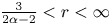 $\frac {3}{2\alpha -2}< r<\infty$ and
 $d=3$. The details are given in §3.
Finally, we show that (1.6) with  $\alpha \geq \frac {7}{4}$ and
 $\eta >0$ always has a unique global solution.
Theorem 1.4 Consider (1.6) with  $\mu >0$,
 $\chi >0$,
 $\eta >0$ and
 $\alpha \geq \frac {7}{4}$. Assume
 $(u_0, w_0, \theta _0)\in H^{s}(\mathbb {R}^{3})$ with
 $s>\frac {5}{2}$ and
 $\nabla \cdot u_0=0$. Then (1.6) has a unique global solution
 $(u, w, \theta )$ satisfying, for any
 $T>0$,
 \[ (u, w, \theta) \in L^{\infty}(0, T; H^{s}(\mathbb{R}^{3})),\quad u\in L^{2}(0, T; H^{s+\alpha}(\mathbb{R}^{3})). \]
Remark 1.5 The assumption  $\alpha \geq \frac {7}{4}$ in theorem 1.4 appears to be sharp. Due to the presence of the term
 $\eta \nabla \nabla \cdot w$, we cannot establish the
 $L^{r}$-bound for
 $w$ with
 $r>2$ as in the proof of theorems 1.1 or 1.2. However, since there is no dissipation in the equation of
 $w$, to obtain the global regularity for this case, it seems necessary to bound
 $\|w\|_{L^{r}(\mathbb {R}^{3})}$ or for a quantity that is close to the regularity level of
 $\|w\|_{L^{r}(\mathbb {R}^{3})}$. For this purpose, one way is to consider the equation of
 $w$ and show the
 $L^{2}$-bound for
 $\Lambda ^{\frac {3}{2}} w$. This eventually yields the minimal assumption
 $\alpha \geq \frac {7}{4}$. It indicates that the presence of the term
 $\eta \nabla \nabla \cdot w$ leads to much more amount dissipation needed than that in the theorem 1.2. For more details, one can refer to the proof of theorem 1.4 in §4.
To prove theorem 1.4, our focus is again on the global a priori bound for  $\|(u, w, \theta )\|_{H^{s}(\mathbb {R}^{3})}$. Due to the presence of the term
 $\eta \nabla \nabla \cdot w$, we develop an approach a little different than in the proof of theorems 1.1 and 1.2. Firstly, there is no difficulty to obtain the global
 $L^{2}$-bound. Secondly, we show an extra regularity on
 $u$, namely
 $\|\Lambda ^{2\alpha -1} u(t)\|_{L^{2}}\in L^{2}(0, T)$, which implies (1.4) with
 $r=2$ and
 $d=3$. Lastly, this extra regularity derives the
 $L^{2}$-bound for
 $\Lambda ^{\frac 32} w$ by combining the equations of
 $u, w, \theta$ and logarithmic type interpolation inequality, which eventually leads to the
 $L^{r}$-bound for
 $w$ with
 $r>2$. These bounds allow us to further obtain the global
 $H^{s}$ bound. The details are given in §4.
Remark 1.6 It is very possible the results above are still valid for the periodic setting. The Littlewood-Paley decomposition, the definitions of the Besov spaces and the logarithmic type Sobolev inequalities have been extended from the whole space to periodic domains (see [Reference Dai, Hu, Wu and Xiao13]). Since these basic ingredients in our paper remain valid and parallel in the periodic setting, it is very reasonable to conclude that these results remain valid for the periodic setting.
Remark 1.7 Another related and interesting model is the Rayleigh-Bénard problem for thermomicropolar fluids (see [Reference Kalita, Łukaszewicz and Siemianowski28])
 \begin{equation} \left\{ \begin{array}{@{}lcl} \partial_t u + u \cdot \nabla u ={-}\nabla p + (\mu + \chi) \Delta u + 2\chi \nabla \times w + \theta \mathbf{e}_d,\\ \partial_t w + u \cdot \nabla w + 4\chi w - \eta \nabla \nabla\cdot w = \nu \Delta w + 2\chi \nabla \times u, \\ \partial_t \theta + u \cdot \nabla \theta = \kappa \Delta \theta + \nabla\times w \cdot \nabla \theta, \\ \nabla \cdot u =0,\\ u(x, 0) =u_0(x), w(x, 0) =w_0(x), \theta(x, 0) =\theta_0(x). \end{array} \right. \end{equation}
The global regularity problem of system (1.8) is more difficult to handle than systems (1.1) and (1.2), since the equation of temperature in (1.8) contains a two derivatives term  $\nabla \times w \cdot \nabla \theta$, while that in (1.1) and (1.2) only contains the convective term
 $u \cdot \mathbf {e}_d$. In fact, if there is only velocity dissipation, namely
 $\mu >0, \chi >0, \nu =0$ and
 $\kappa =0$, we even cannot obtain the global a priori
 $L^{2}$-bound for the solution
 $(u, w, \theta )$ of (1.8). Therefore, to establish the global regularity of solutions to (1.8), one needs dissipation in the equation of
 $w$ or
 $\theta$, which is left to be investigated in future.
The rest of this paper is organized as follows. Sections 2–4 are devoted to the proofs of theorems 1.1, 1.2 and 1.4, respectively. The Littlewood-Paley decomposition, the definition of Besov spaces, several calculus inequalities and logarithmic type Besov interpolation inequalities are given in the Appendix. To simplify the notation, we will write  $\int f$ for
 $\int _{\mathbb {R}^{d}} f(x) dx$,
 $\|f\|_{L^{r}}$ for
 $\|f\|_{L^{r}(\mathbb {R}^{d})}$,
 $\|f\|_{H^{s}}$ for
 $\|f\|_{H^{s}(\mathbb {R}^{d})}$, and
 $\|f\|_{B_{p, q}^{s}}$ for
 $\|f\|_{B_{p, q}^{s}(\mathbb {R}^{d})}$.
2. Proof of theorem 1.1
This section is devoted to the proof of theorem 1.1, stating the global existence and uniqueness of solutions to the 2D micropolar Rayleigh-Bénard problem (1.3). The general approach to establish the global existence and regularity results consists of two main steps. The first step assesses the local (in time) well-posedness while the second extends the local solution into a global one by obtaining global (in time) a priori bounds. For the system of equations concerned here, the local well-posedness follows from standard approach such as Friedrichs method (see, e.g., [Reference Xu, Qiao and Zhang53] in  $\mathbb {R}^{2}$). Therefore, the key step to show theorem 1.1 is to establish the global a priori bound on the solution
 $(u, w, \theta )$ in
 $H^{s}$. More precisely, we prove the following main proposition.
Proposition 2.1 Consider (1.3) with  $\mu >0$ and
 $\chi >0$. Assume
 $(u_0, w_0, \theta _0)\in H^{s}(\mathbb {R}^{2})$ with
 $s>2$ and
 $\nabla \cdot u_0=0$. Then the corresponding solution
 $(u, w, \theta )$ of (1.3) is globally bounded in
 $H^{s}(\mathbb {R}^{2})$.
The proof of proposition 2.1 requires several steps. For the sake of clarity, we divide the rest of this section into three subsections.
2.1 Global  $L^{2}$-bound for $(u, w)$ and global bound for $\|\theta \|_{L^{r}}$


This subsection provides the global  $L^{2}$-bound and a global bound for
 $\|\theta \|_{L^{r}}$ with
 $r\geq 2$. More precisely, we have the following proposition.
Proposition 2.2 Let  $(u, w, \theta )$ be the corresponding solution of (1.3). Then,
 $(u, w, \theta )$ obeys the following global bounds, for any
 $T>0$ and
 $0< t< T$,
 \begin{align} &\|u(t)\|_{L^{2}}^{2} + \|w(t)\|_{L^{2}}^{2} + \|\theta(t)\|_{L^{2}}^{2} + \int_{0}^{t} \|\nabla u(\tau)\|_{L^{2}}^{2}\,\textrm{d}\tau\leq C(T, u_0, w_0, \theta_0)<\infty, \end{align}
 \begin{align} &\|\theta(t)\|_{L^{r}}\leq C(T, u_0, w_0, \theta_0)<\infty, \end{align}
with  $r\geq 2$.
Proof. To obtain the global  $L^{2}$-bound (2.1), we dot (1.3) with
 $(u, w, \theta )$ to obtain
 \begin{align*} &\frac{1}{2} \frac{\textrm{d}}{\textrm{d}t} (\|u(t)\|_{L^{2}}^{2} + \|w(t)\|_{L^{2}}^{2} + \|\theta(t)\|_{L^{2}}^{2}) + (\mu + \chi)\|\nabla u\|^{2}_{L^{2}} + 4\chi\|w\|^{2}_{L^{2}}\nonumber\\ &\quad= 4 \chi \int (\nabla\times u)\cdot w + \int \theta \mathbf{e}_2\cdot u + \int u\cdot\mathbf{e}_2 \theta\nonumber\\ &\quad\leq 4\chi \|\nabla u\|_{L^{2}} \|w\|_{L^{2}} + 2\|u_2\|_{L^{2}} \|\theta\|_{L^{2}}\nonumber\\ &\quad\leq \chi \|\nabla u\|_{L^{2}}^{2} + 4\chi \|w\|_{L^{2}}^{2} + \|u\|_{L^{2}}^{2} + \|\theta\|_{L^{2}}^{2}, \end{align*}
where we have used the Young inequality in the last inequality. This, together with Gronwall's inequality, then leads to the desired bound (2.1).
Now we start to show (2.2). Multiplying the third equation in (1.3) by  $\theta |\theta |^{r-2}$, and integrating in space domain, together with Hölder's inequality, we obtain
 \begin{align*} \frac 1r \frac{\textrm{d}}{\textrm{d}t}\|\theta(t)\|_{L^{r}}^{r} &= \int u_2 \theta |\theta|^{r-2}\\ &\leq \|u_2(t)\|_{L^{r}} \|\theta(t)\|_{L^{r}}^{r-1}. \end{align*}
Integrating this in  $[0, t]$, together with (2.1), we derive that
 \begin{align} \|\theta(t)\|_{L^{r}}&\leq \|\theta_0\|_{L^{r}} + \int_0^{t} \|u(\tau)\|_{L^{r}}\,\textrm{d}\tau \end{align}
 \begin{align} &\leq C + C \int_0^{t} (\|u(\tau)\|_{L^{2}} + \|\nabla u(\tau)\|_{L^{2}})\,\textrm{d}\tau \end{align}
 \begin{align} &\leq C. \end{align}
Thus the proof of proposition 2.2 is completed.
2.2 Global bounds for $\|(\nabla u, w)\|_{L^{r}}$, $\|(u, \theta )\|_{L^{\infty }}$ and global time integrability $\|\nabla \times u\|_{B_{\infty , \infty }^{0}}$


The major result of this subsection is the global bound stated in the following proposition.
Proposition 2.3 Assume that  $(u, w, \theta )$ solves (1.3). Then,
 $(u, w, \theta )$ obeys the following global a priori bounds, for any
 $T>0$ and
 $0< t< T$,
 \begin{align} \|\nabla u(t)\|_{L^{r}} &\leq C(T, u_0, w_0, \theta_0) < \infty\ for\ any\ 2\leq r <\infty; \end{align}
 \begin{align} \|w(t)\|_{L^{r}} &\leq C(T, u_0, w_0, b_0) <\infty\ for\ any\ 2\leq r \leq\infty; \end{align}
 \begin{align} \|u(t)\|_{L^{r}} &\leq C(T, u_0, w_0, b_0) <\infty\ for\ any\ 2\leq r \leq\infty; \end{align}
 \begin{align} \|\theta(t)\|_{L^{\infty}} &\leq C(T, u_0, w_0, b_0) <\infty; \end{align}
 \begin{align} \int_0^{t} \|\nabla\times u(\tau)\|_{B_{\infty, \infty}^{0}}\,\textrm{d}\tau &\leq C(T, u_0, w_0, \theta_0) < \infty. \end{align}
Proof. To obtain these global bounds, we make use of the equation of vorticity  $\Omega =\nabla \times u$,
 \begin{equation} \partial_t \Omega + u\cdot \nabla\Omega - (\mu + \chi)\Delta\Omega ={-} 2\chi \Delta w + \partial_{x_1} \theta. \end{equation}
It appears that direct energy estimates on (2.11) would not lead to the desired global bound, due to the presence of the bad terms  $-\Delta w$ and
 $\partial _{x_1} \theta$. The idea here is to hide these terms by working with two new combined quantities. More precisely, we set
 \begin{equation} \mathcal{R} = (-\Delta)^{{-}1} \partial_{x_1}, \quad \mathcal{F} = \Omega - \frac{2 \chi}{\mu + \chi} w, \quad \mathcal{G} = \mathcal{F} - \frac{1}{\mu + \chi} \mathcal{R} \theta. \end{equation}
The vorticity equation (2.11) becomes
 \begin{equation} \partial_t \Omega + u\cdot \nabla \Omega - (\mu + \chi) \Delta \mathcal{F} = \partial_{x_1} \theta, \end{equation}
and
 \begin{equation} \partial_t \Omega + u\cdot \nabla \Omega - (\mu + \chi) \Delta \mathcal{G} = 0. \end{equation}
To obtain equations for  $\mathcal {F}$ and
 $\mathcal {G}$, we multiply the second equation in (1.3) by
 $\frac {2 \chi }{\mu + \chi }$, and apply
 $\frac {1}{\mu + \chi } \mathcal {R}$ to the third equation in (1.3) to get
 \begin{equation} \partial_t \left(\frac{2 \chi}{\mu + \chi} w\right) + u \cdot \nabla \left(\frac{2 \chi}{\mu + \chi} w\right) = \frac{4 \chi^{2}}{\mu + \chi} \mathcal{F} - \frac{8 \mu \chi^{2}}{\mu + \chi} w, \end{equation}
and
 \begin{equation} \partial_t \left(\frac{1}{\mu + \chi} \mathcal{R} \theta\right) + u \cdot \nabla \left(\frac{1}{\mu + \chi} \mathcal{R} \theta\right) = \frac{1}{\mu + \chi} \mathcal{R} (u \cdot \mathbf{e}_2) - \frac{1}{\mu + \chi} [\mathcal{R}, u\cdot \nabla]\theta. \end{equation}
 \begin{equation} \partial_t \mathcal{F} + u\cdot \nabla \mathcal{F} - (\mu + \chi) \Delta \mathcal{F} + \frac{4 \chi^{2}}{\mu + \chi} \mathcal{F} = \partial_{x_1} \theta + \frac{8 \mu \chi^{2}}{\mu + \chi} w, \end{equation}
and
 \begin{align} & \partial_t \mathcal{G} + u\cdot \nabla \mathcal{G} - (\mu + \chi) \Delta \mathcal{G} + \frac{4 \chi^{2}}{\mu + \chi} \mathcal{G}\nonumber\\ &\quad= \frac{1}{\mu + \chi} [\mathcal{R}, u\cdot \nabla]\theta - \frac{1}{\mu + \chi} \mathcal{R} (u \cdot \mathbf{e}_2) + \frac{8 \mu \chi^{2}}{\mu + \chi} w - \frac{4 \chi^{2}}{(\mu + \chi)^{2}} \mathcal{R} \theta. \end{align}
We first show (2.6) with  $r=2$, namely
 $\|\nabla u\|_{L^{2}}\leq C$. To this end, we take the inner product of (2.17) with
 $\mathcal {F}$ to yield
 \[ \frac{1}{2}\frac{\textrm{d}}{\textrm{d}t} \|\mathcal{F}\|_{L^{2}}^{2} + (\mu + \chi) \|\nabla \mathcal{F}\|_{L^{2}}^{2} \leq \int \partial_{x_1} \theta \mathcal{F} + \frac{8 \mu \chi^{2}}{\mu + \chi} \int w \mathcal{F}. \]
Using integration by parts, Hölder's inequality and the Young inequality, we derive that
 \[ \int \partial_{x_1} \theta \mathcal{F} ={-} \int \theta \partial_{x_1} \mathcal{F} \leq \|\theta\|_{L^{2}} \|\partial_{x_1} \mathcal{F}\|_{L^{2}} \leq \frac{\mu + \chi}{2} \|\nabla \mathcal{F}\|_{L^{2}}^{2} + C \|\theta\|_{L^{2}}^{2}. \]
Similarly, we have
 \[ \frac{8 \mu \chi^{2}}{\mu + \chi} \int w \mathcal{F} \leq \frac{4 \mu \chi^{2}}{\mu + \chi} (\|w\|_{L^{2}}^{2} + \|\mathcal{F}\|_{L^{2}}^{2}). \]
We thus have obtained
 \[ \frac{\textrm{d}}{\textrm{d}t} \|\mathcal{F}\|_{L^{2}}^{2} + (\mu + \chi) \|\nabla \mathcal{F}\|_{L^{2}}^{2} \leq C \|\mathcal{F}\|_{L^{2}}^{2} + C (\|w\|_{L^{2}}^{2} + \|\theta\|_{L^{2}}^{2}). \]
Then this together with Gronwall's inequality and (2.1) leads to
 \[ \|\mathcal{F}(t)\|_{L^{2}}^{2} \leq C. \]
Thus (2.6) with  $r=2$ follows from this estimate, the definition of
 $\mathcal {F}$, (2.1) and
 $\|\nabla u\|_{L^{2}}=\|\Omega \|_{L^{2}}$. As a product, we have for any
 $2\leq r<\infty$,
 \begin{equation} \|u(t)\|_{L^{r}} \leq C. \end{equation}
We now estimate  $\|\nabla u\|_{L^{r}}$ and
 $\|w\|_{L^{r}}$ with
 $r>2$. Multiplying (2.18), (1.3)
 $_2$ and (2.16) by
 $\mathcal {G} |\mathcal {G}|^{r-2}$,
 $w |w|^{r-2}$ and
 $\mathcal {R} \theta |\mathcal {R} \theta |^{r-2}$, respectively, integrating the results in space domain and adding them up, we obtain
 \begin{align} &\frac{1}{r}\frac{\textrm{d}}{\textrm{d}t} (\|\mathcal{G}\|_{L^{r}}^{r} + \|w\|_{L^{r}}^{r} + \|\mathcal{R} \theta\|_{L^{r}}^{r})\nonumber\\ &\quad\leq \frac{1}{\mu + \chi} \int [\mathcal{R}, u\cdot \nabla]\theta \mathcal{G} |\mathcal{G}|^{r-2} - \frac{1}{\mu + \chi} \int \mathcal{R} (u \cdot \mathbf{e}_2) \mathcal{G} |\mathcal{G}|^{r-2} + \frac{8 \mu \chi^{2}}{\mu + \chi} \int w \mathcal{G} |\mathcal{G}|^{r-2}\nonumber\\ &\qquad- \frac{4 \chi^{2}}{(\mu + \chi)^{2}} \int \mathcal{R} \theta \mathcal{G} |\mathcal{G}|^{r-2} + 2 \chi \int \mathcal{G} w |w|^{r-2} + \frac{2 \chi}{\mu + \chi} \int \mathcal{R} \theta w |w|^{r-2}\nonumber\\ &\qquad+\int \mathcal{R} (u \cdot \mathbf{e}_2) \mathcal{R} \theta |\mathcal{R} \theta|^{r-2} - \int [\mathcal{R}, u\cdot \nabla]\theta \mathcal{R} \theta |\mathcal{R} \theta|^{r-2}\nonumber\\ &\quad:= I_1 + I_2 + I_3 + I_4 + I_5 + I_6 + I_7 + I_8. \end{align}
The terms on the right can be estimated as follows. Using Hölder's inequality, Riesz's theorem and the Young inequality, one infers that
 \begin{align*} |I_1| &\leq \frac{1}{\mu + \chi} \|[\mathcal{R}, u\cdot \nabla]\theta\|_{L^{r}} \|\mathcal{G}\|_{L^{r}}^{r-1}\\ &\leq C \|u\|_{L^{2r}} \|\theta\|_{L^{2r}} \|\mathcal{G}\|_{L^{r}}^{r-1}\\ &\leq C(\|u\|_{L^{2r}}^{r} \|\theta\|_{L^{2r}}^{r} + \|\mathcal{G}\|_{L^{r}}^{r}). \end{align*}
Similarly, we have
 \[ |I_8| \leq C (\|u\|_{L^{2r}}^{r} \|\theta\|_{L^{2r}}^{r} + \|\mathcal{R} \theta\|_{L^{r}}^{r}). \]
Again applying Hölder's inequality and Riesz's theorem,
 \begin{align*} |I_2| &\leq \frac{1}{\mu + \chi} \|\mathcal{R} (u \cdot \mathbf{e}_2)\|_{L^{r}} \|\mathcal{G}\|_{L^{r}}^{r-1}\\ &\leq C (\|\mathcal{R} u\|_{L^{r}}^{r} + \|\mathcal{G}\|_{L^{r}}^{r}). \end{align*}
By the Young inequality,
 \begin{align*} |I_3| &\leq \frac{8 \mu \chi^{2}}{\mu + \chi} \|w\|_{L^{r}} \|\mathcal{G}\|_{L^{r}}^{r-1}\\ &\leq C (\|w\|_{L^{r}}^{r} + \|\mathcal{G}\|_{L^{r}}^{r}). \end{align*}
Similarly, we have
 \begin{align*} |I_4| &\leq C (\|\mathcal{R} \theta\|_{L^{r}}^{r} + \|\mathcal{G}\|_{L^{r}}^{r}). |I_5| \leq C (\|\mathcal{G}\|_{L^{r}}^{r} + \|w\|_{L^{r}}^{r}).\\ |I_6| &\leq C (\|\mathcal{R} \theta\|_{L^{r}}^{r} + \|w\|_{L^{r}}^{r}). |I_7| \leq C (\|\mathcal{R} u\|_{L^{r}}^{r} + \|\mathcal{R} \theta\|_{L^{r}}^{r}). \end{align*}
Substituting the above bounds into (2.20), leads to
 \begin{align} &\frac{\textrm{d}}{\textrm{d}t} (\|\mathcal{G}\|_{L^{r}}^{r} + \|w\|_{L^{r}}^{r} + \|\mathcal{R} \theta\|_{L^{r}}^{r})\nonumber\\ &\quad\leq C (\|u\|_{L^{2r}}^{r} \|\theta\|_{L^{2r}}^{r} + \|\mathcal{R} u\|_{L^{r}}^{r}) + C (\|\mathcal{G}\|_{L^{r}}^{r} + \|w\|_{L^{r}}^{r} + \|\mathcal{R} \theta\|_{L^{r}}^{r})\nonumber\\ &\quad\leq C (1 + \|\mathcal{R} u\|_{L^{r}}^{r}) + C (\|\mathcal{G}\|_{L^{r}}^{r} + \|w\|_{L^{r}}^{r} + \|\mathcal{R} \theta\|_{L^{r}}^{r}), \end{align}
where we have used (2.2) and (2.19) in the last inequality. To close the estimate (2.21), we further need to bound  $\|\mathcal {R} u\|_{L^{r}}$. To this end, applying
 $\mathcal {R}$ to the first equation in (1.3), dotting the result with
 $\mathcal {R} u |\mathcal {R} u|^{r-2}$ and integrating it in space domain, we obtain
 \begin{align} \frac{1}{r}\frac{\textrm{d}}{\textrm{d}t} \|\mathcal{R} u\|_{L^{r}}^{r}&\leq \int \mathcal{R} (u\cdot \nabla u) \cdot \mathcal{R} u |\mathcal{R} u|^{r-2} + \int \mathcal{R} (\theta \mathbf{e}_2) \cdot \mathcal{R} u |\mathcal{R} u|^{r-2}\nonumber\\ &= \int \mathcal{R} \nabla\cdot \sum_{i, j=1}^{2}(u_i u_j) \cdot \mathcal{R} u |\mathcal{R} u|^{r-2} + \int \mathcal{R} (\theta \mathbf{e}_2) \cdot \mathcal{R} u |\mathcal{R} u|^{r-2}\nonumber\\ &\leq C (\|u\|_{L^{2r}}^{2} + \|\mathcal{R} \theta\|_{L^{r}}) \|\mathcal{R} u\|_{L^{r}}^{r-1}\nonumber\\ &\leq C (1 + \|\mathcal{R} \theta\|_{L^{r}}^{r} + \|\mathcal{R} u\|_{L^{r}}^{r}). \end{align}
 \begin{align} &\frac{\textrm{d}}{\textrm{d}t} (\|\mathcal{G}\|_{L^{r}}^{r} + \|w\|_{L^{r}}^{r} + \|\mathcal{R} \theta\|_{L^{r}}^{r} + \|\mathcal{R} u\|_{L^{r}}^{r})\nonumber\\ &\quad\leq C + C (\|\mathcal{G}\|_{L^{r}}^{r} + \|w\|_{L^{r}}^{r} + \|\mathcal{R} \theta\|_{L^{r}}^{r} + \|\mathcal{R} u\|_{L^{r}}^{r}). \end{align}
Gronwall's inequality then implies that
 \begin{equation} \|\mathcal{G}(t)\|_{L^{r}}^{r} + \|w(t)\|_{L^{r}}^{r} + \|\mathcal{R} \theta(t)\|_{L^{r}}^{r} + \|\mathcal{R} u(t)\|_{L^{r}}^{r}\leq C. \end{equation}
This yields (2.7) with  $2< r<\infty$. Furthermore, (2.6) with
 $2< r<\infty$ follows from (2.24), the definition of
 $\mathcal {G}$ and
 $\|\nabla u\|_{L^{r}}\leq C\|\Omega \|_{L^{r}}$. As a product, we obtain (2.6) with
 $r=\infty$. In fact, for any
 $r>2$,
 \begin{equation} \|u\|_{L^{\infty}}\leq C(\|u\|_{L^{2}} + \|\nabla u\|_{L^{r}})\leq C. \end{equation}
This, together with (2.3) with  $r=\infty$, implies (2.9), namely
 $\|\theta \|_{L^{\infty }}\leq C$.
Finally, to bound  $\int _0^{t} \|\nabla \times u(\tau )\|_{B_{\infty , \infty }^{0}}\,\textrm {d}\tau$ and
 $\|w\|_{L^{\infty }}$, we shall take advantage of Littlewood-Payley decomposition. By high-low frequencies decomposition, together with the estimates (2.6) and (2.7), we have for any
 $2\leq r<\infty$,
 \begin{align} \int_0^{t} \|\mathcal{F}(\tau)\|_{B_{r, 1}^{\frac{2}{r}}}\,\textrm{d}\tau & \leq \sum_{j={-}1}^{N-1} 2^{\frac{2}{r} j} \int_0^{t} \|\Delta_j \mathcal{F}(\tau)\|_{L^{r}}\,\textrm{d}\tau + \sum_{j\geq N} 2^{\frac{2}{r} j} \int_0^{t} \|\Delta_j \mathcal{F}(\tau)\|_{L^{r}}\,\textrm{d}\tau\nonumber\\ & \leq C 2^{\frac{2}{r}N} \int_0^{t} \|\mathcal{F}(\tau)\|_{L^{r}}\,\textrm{d}\tau + \sum_{j\geq N} 2^{\frac{2}{r}j} \int_0^{t} \|\Delta_j \mathcal{F}(\tau)\|_{L^{r}}\,\textrm{d}\tau\nonumber\\ & \leq C 2^{\frac{2}{r}N} + \sum_{j\geq N} 2^{\frac{2}{r} j} \int_0^{t} \|\Delta_j \mathcal{F}(\tau)\|_{L^{r}}\,\textrm{d}\tau, \end{align}
where the positive integer  $N$ is to be fixed.
Now we start to bound the second term on the right of (2.26). Applying  $\Delta _j$ to (2.17), multiplying the resulting equation by
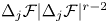 $\Delta _j \mathcal {F} |\Delta _j \mathcal {F}|^{r-2}$, and then integrating it in space domain, yields
 \begin{align} &\frac{1}{r}\frac{\textrm{d}}{\textrm{d}t}\|\Delta_j \mathcal{F}\|_{L^{r}}^{r} + \int \Delta_j \Delta \mathcal{F} \Delta_j \mathcal{F}|\Delta_j \mathcal{F}|^{r-2} \nonumber\\ &\quad\leq \int \Delta_j \partial_{x_1} \theta \Delta_j \mathcal{F}|\Delta_j \mathcal{F}|^{r-2} + \frac{8 \mu \chi^{2}}{\mu + \chi} \int \Delta_j w \Delta_j \mathcal{F}|\Delta_j \mathcal{F}|^{r-2}\notag\\ &\quad - \int [\Delta_j, u\cdot \nabla] \mathcal{F} \Delta_j \mathcal{F}|\Delta_j \mathcal{F}|^{r-2}\nonumber\\ &\quad\leq C(\|\Delta_j \partial_{x_1} \theta\|_{L^{r}} + \|\Delta_j w\|_{L^{r}}) \|\Delta_j \mathcal{F}\|_{L^{r}}^{r-1} + \|[\Delta_j, u\cdot \nabla] \mathcal{F}\|_{L^{r}} \|\Delta_j \mathcal{F}\|_{L^{r}}^{r-1}\nonumber\\ &\quad\leq C 2^{j} \|\Delta_j \mathcal{F}\|_{L^{r}}^{r-1} + \|[\Delta_j, u\cdot \nabla] \mathcal{F}\|_{L^{r}} \|\Delta_j \mathcal{F}\|_{L^{r}}^{r-1}, \end{align}
where we have used Bernstein's inequality, (2.2) and (2.7) in the last inequality. The dissipative term admits the lower bound (see, e.g., [Reference Chen, Miao and Zhang11])
 \begin{equation} \int \Delta_j \Delta \mathcal{F} \Delta_j \mathcal{F}|\Delta_j \mathcal{F}|^{r-2} \geq c_0 2^{2j}\|\Delta_j \mathcal{F}\|_{L^{r}}^{r}, \end{equation}
for a pure constant  $c_0>0$.
Inserting (2.28) into (2.27), we derive that
 \begin{equation} \frac{\textrm{d}}{\textrm{d}t}\|\Delta_j \mathcal{F}\|_{L^{r}} + c_0 2^{2j}\|\Delta_j \mathcal{F}\|_{L^{r}}\leq C 2^{j} + \|[\Delta_j, u\cdot \nabla] \mathcal{F}\|_{L^{r}}. \end{equation}
By the commutator estimate, lemma A.4, together with (2.6), leads to
 \begin{equation} \|[\Delta_j, u\cdot \nabla] \mathcal{F}\|_{L^{r}} \leq C \|\nabla u\|_{L^{r}} \|\mathcal{F}\|_{L^{\infty}} \leq C \|\mathcal{F}\|_{B_{r, 1}^{\frac{2}{r}}}. \end{equation}
Combining (2.29) and (2.30) yields
 \[ \frac{\textrm{d}}{\textrm{d}t}\|\Delta_j \mathcal{F}\|_{L^{r}} + c_0 2^{2j}\|\Delta_j \mathcal{F}\|_{L^{r}}\leq C 2^{j} + C \|\mathcal{F}\|_{B_{r, 1}^{\frac{2}{r}}}. \]
Integrating this with respect to time,
 \begin{equation} \|\Delta_j \mathcal{F}(t)\|_{L^{r}} \leq \textrm{e}^{- c_0 2^{2j} t} \|\Delta_j \mathcal{F}_0\|_{L^{r}} + C \int_0^{t}\,\textrm{e}^{- c_0 2^{2j} (t-\tau)} (2^{j} + \|\mathcal{F}(\tau)\|_{B_{r, 1}^{\frac{2}{r}}})\,\textrm{d}\tau. \end{equation}
Taking  $L^{1}$ norm in
 $[0, t]$ to (2.31), applying the Young inequality for the time convolution and multiplying the result by
 $2^{\frac {2}{r} j}$, we find
 \begin{align*} 2^{\frac{2}{r} j} \int_0^{t} \|\Delta_j \mathcal{F}(\tau)\|_{L^{r}}\,\textrm{d}\tau &\leq C 2^{-(2 - \frac{2}{r}) j} \|\Delta_j \mathcal{F}_0\|_{L^{r}} + C 2^{-\left(1 - \frac{2}{r}\right) j}\\ &\quad + C 2^{-\left(2 - \frac{2}{r}\right) j} \int_0^{t} \|\mathcal{F}(\tau)\|_{B_{r, 1}^{\frac{2}{r}}}\,\textrm{d}\tau. \end{align*}
Taking the sum over  $j\geq N$, note that
 $r>2$ and
 $1-\frac {2}{r} >0$, it infers that
 \begin{align*} \sum_{j\geq N} 2^{\frac{2}{r} j} \int_0^{t} \|\Delta_j \mathcal{F}(\tau)\|_{L^{r}}\,\textrm{d}\tau &\leq C \|\mathcal{F}_0\|_{L^{r}} + C 2^{-\left(1 - \frac{2}{r}\right) N}\\ &\quad + C_0 2^{-\left(2 - \frac{2}{r}\right) N} \int_0^{t} \|\mathcal{F}(\tau)\|_{B_{r, 1}^{\frac{2}{r}}}\,\textrm{d}\tau. \end{align*}
Substituting this into (2.26), and choosing  $N$ sufficiently large such that
 \[ C_0 2^{- \left(2 - \frac{2}{r}\right) N} \leq \frac{1}{2}, \]
we derive that
 \begin{equation} \int_0^{t} \|\mathcal{F}(\tau)\|_{B_{r, 1}^{\frac{2}{r}}}\,\textrm{d}\tau \leq C. \end{equation}
Multiply (1.3) $_2$ by
 $w |w|^{r-2}$ and integrating in space domain, we obtain
 \begin{align*} \frac{1}{r} \frac{\textrm{d}}{\textrm{d}t} \|w\|_{L^{r}}^{r} + 4 \mu \chi \|w\|_{L^{r}}^{r} &= 2 \chi \int \nabla\times u w |w|^{r-2}\\ &\leq 2 \chi \|\Omega\|_{L^{r}} \|w\|_{L^{r}}^{r-1}. \end{align*}
Integrating this with respect to time, and taking  $r\rightarrow \infty$, yields
 \begin{equation} \|w(t)\|_{L^{\infty}} \leq C \int_0^{t} \|\Omega(\tau)\|_{L^{\infty}}\,\textrm{d}\tau. \end{equation}
By the definition of  $\mathcal {F}$, note that
 $\|\mathcal {F}\|_{L^{\infty }}\leq C \|\mathcal {F}\|_{B_{r, 1}^{\frac {2}{r}}}$, we get from (2.32) and (2.33),
 \begin{align} \|w(t)\|_{L^{\infty}} &\leq C \int_0^{t} (\|\mathcal{F}(\tau)\|_{L^{\infty}} + \|w(\tau)\|_{L^{\infty}})\,\textrm{d}\tau\nonumber\\ &\leq C + C \int_0^{t} \|w(\tau)\|_{L^{\infty}}\,\textrm{d}\tau. \end{align}
Then Gronwall's inequality leads to
 \begin{equation} \int_0^{t} \|w(\tau)\|_{L^{\infty}}\,\textrm{d}\tau\leq C. \end{equation}
 \begin{align} \int_0^{t} \|\Omega(\tau)\|_{B_{\infty, \infty}^{0}}\,\textrm{d}\tau&\leq \int_0^{t} \|\Omega(\tau)\|_{L^{\infty}}\,\textrm{d}\tau \leq \int_0^{t} \|\mathcal{F}(\tau)\|_{L^{\infty}}\,\textrm{d}\tau\notag\\ &\quad + \frac{2 \chi}{\mu + \chi} \int_0^{t} \|w(\tau)\|_{L^{\infty}}\,\textrm{d}\tau\leq C, \end{align}
which is (2.10). Finally, substituting (2.36) into (2.33) infers that (2.7) with  $r=\infty$. We thus complete the proof of proposition 2.3.
2.3 Global $H^{s}$ bound

This subsection completes the proof of proposition 2.1 by establishing the global  $H^{s}$ bound.
Proof of proposition 2.1. Applying  $\Lambda ^{s}$ to the equations in (1.3) and taking
 $L^{2}$-inner product to the resulting equations with
 $(\Lambda ^{s} u, \Lambda ^{s} w, \Lambda ^{s} \theta )$ yields
 \begin{align} &\frac{1}{2}\frac{\textrm{d}}{\textrm{d}t} (\|\Lambda^{s} u\|_{L^{2}}^{2} + \|\Lambda^{s} w\|_{L^{2}}^{2} + \|\Lambda^{s} \theta\|_{L^{2}}^{2}) + (\mu + \chi) \|\Lambda^{s+1} u\|_{L^{2}}^{2}\nonumber\\ &\quad\leq{-}\int [\Lambda^{s}, u\cdot\nabla] u \cdot \Lambda^{s} u + 2 \chi \int \Lambda^{s} \nabla\times w\cdot \Lambda^{s} u\notag\\ &\qquad + \int \Lambda^{s}(\theta \mathbf{e}_2)\cdot\Lambda^{s} u -\int [\Lambda^{s}, u\cdot\nabla] w \cdot \Lambda^{s} w\nonumber\\ &\qquad+ 2 \chi \int \Lambda^{s} \nabla\times u\cdot \Lambda^{s} w -\int [\Lambda^{s}, u\cdot\nabla] \theta \cdot \Lambda^{s} \theta + \int \Lambda^{s}(u\cdot \mathbf{e}_2) \Lambda^{s} \theta\nonumber\\ &\quad:=J_1 + J_2 + J_3 + J_4 + J_5 + J_6 + J_7. \end{align}
The terms on the right-hand side can be estimated as follows. By Hölder's inequality and lemma A.3,
 \begin{align*} |J_1| &\leq C \|[\Lambda^{s}, u\cdot\nabla] u\|_{L^{2}} \|\Lambda^{s} u\|_{L^{2}}\\ &\leq C \|\nabla u\|_{L^{\infty}} \|\Lambda^{s} u\|_{L^{2}}^{2}. \end{align*}
By Hölder's inequality and the Young inequality,
 \begin{align*} |J_2+J_5| &\leq C \|\Lambda^{s} w\|_{L^{2}} \|\Lambda^{s+1} u\|_{L^{2}}\leq \frac{\mu + \chi}{8} \|\Lambda^{s+1} u\|_{L^{2}}^{2} + C \|\Lambda^{s} w\|_{L^{2}}^{2}.\\ |J_3+J_7| &\leq C\|\Lambda^{s} u\|_{L^{2}} \|\Lambda^{s} \theta\|_{L^{2}}\leq C(\|\Lambda^{s} u\|_{L^{2}}^{2} + \|\Lambda^{s} \theta\|_{L^{2}}^{2}). \end{align*}
Again using Hölder's inequality, the Young inequality and commutator estimate lemma A.3,
 \begin{align*} |J_4| &\leq C \|[\Lambda^{s}, u\cdot\nabla] w\|_{L^{2}} \|\Lambda^{s} w\|_{L^{2}}\\ &\leq C (\|\nabla u\|_{L^{\infty}} \|\Lambda^{s} w\|_{L^{2}} + \|w\|_{L^{\infty}} \|\Lambda^{s+1} u\|_{L^{2}}) \|\Lambda^{s} w\|_{L^{2}}\\ &\leq \frac{\mu + \chi}{8} \|\Lambda^{s+1} u\|_{L^{2}}^{2} + C (\|\nabla u\|_{L^{\infty}} + \|w\|_{L^{\infty}}^{2}) \|\Lambda^{s} w\|_{L^{2}}^{2}. \end{align*}
Similarly, we have
 \[ |J_6|\leq \frac{\mu + \chi}{8} \|\Lambda^{s+1} u\|_{L^{2}}^{2} + C (\|\nabla u\|_{L^{\infty}} + \|\theta\|_{L^{\infty}}^{2}) \|\Lambda^{s} \theta\|_{L^{2}}^{2}. \]
Inserting the bounds above in (2.37), we have
 \begin{align} &\frac{\textrm{d}}{\textrm{d}t} (\|\Lambda^{s} u\|_{L^{2}}^{2} + \|\Lambda^{s} w\|_{L^{2}}^{2} + \|\Lambda^{s} \theta\|_{L^{2}}^{2}) + (\mu + \chi) \|\Lambda^{s+1} u\|_{L^{2}}^{2}\nonumber\\ &\quad\leq C (1 + \|\nabla u\|_{L^{\infty}} + \|w\|_{L^{\infty}}^{2} + \|\theta\|_{L^{\infty}}^{2}) (\|\Lambda^{s} u\|_{L^{2}}^{2} + \|\Lambda^{s} w\|_{L^{2}}^{2} + \|\Lambda^{s} \theta\|_{L^{2}}^{2})\nonumber\\ &\quad\leq C (1 + \|\nabla u\|_{L^{\infty}}) (\|\Lambda^{s} u\|_{L^{2}}^{2} + \|\Lambda^{s} w\|_{L^{2}}^{2} + \|\Lambda^{s} \theta\|_{L^{2}}^{2})\nonumber\\ &\quad\leq C (1 + (1+ \|\nabla\times u\|_{B_{\infty, \infty}^{0}}) \log(e+ \|\Lambda^{s} u\|_{L^{2}}))\notag\\ &\qquad \times (\|\Lambda^{s} u\|_{L^{2}}^{2} + \|\Lambda^{s} w\|_{L^{2}}^{2} + \|\Lambda^{s} \theta\|_{L^{2}}^{2}). \end{align}
where we have used (2.7) and (2.9) in the second inequality, and lemma A.6 in the last inequality. We thus obtain the desired global  $H^{s}$-bound after applying (2.10) and Osgood's inequality, which states that a differential inequality on a nonnegative function
 $f$,
 \[ \frac{\textrm{d}f}{\textrm{d}t} \leq a(t) f(t) \log(e + f(t)) \]
implies that  $f=f(t)$ is bounded on
 $[0, T]$ if the nonnegative function
 $a=a(t)$ is integrable on
 $[0,T]$. This completes the proof of proposition 2.1.
3. Proof of theorem 1.2
This section proves theorem 1.2. As we know, it suffices to establish the global a priori estimates on the  $H^{s}$-norm of the solution
 $(u, w, \theta )$ to (1.6), which is obtained in the following proposition.
Proposition 3.1 Consider (1.6) with  $\mu >0$,
 $\chi >0$,
 $\eta =0$ and
 $\alpha \geq \frac {5}{4}$. Assume
 $(u_0, w_0, \theta _0)\in H^{s}(\mathbb {R}^{3})$ with
 $s>\frac {5}{2}$ and
 $\nabla \cdot u_0=0$. Then the corresponding solution
 $(u, w, \theta )$ of (1.6) is globally bounded in
 $H^{s}(\mathbb {R}^{3})$.
We will prove proposition 3.1 for the case  $\frac {5}{4}\leq \alpha < \frac {5}{2}$. The case
 $\alpha \geq \frac {5}{2}$ can be treated similarly. The proof is slightly long. For the sake of clarity, we divide the rest of this section into three subsections.
3.1 Global $L^{2}$-bound for $(u, w, \theta )$ and global time integrability for $\|\Lambda ^{\rho +\alpha } u\|_{L^{2}}^{2}$


This subsection provides the global  $L^{2}$-bound and a global time integrability for
 $\|\Lambda ^{\rho +\alpha } u\|_{L^{2}}^{2}$ for any
 $0\leq \rho \leq \alpha -1$. More precisely, we first state the following proposition in terms of the global
 $L^{2}$-bound.
Proposition 3.2 Assume that  $(u, w, \theta )$ solves (1.6). Then for any
 $t>0$,
 $(u, w, \theta )$ obeys the following global
 $L^{2}$ bound,
 \begin{equation} \|u\|_{L^{2}}^{2} + \|w\|_{L^{2}}^{2} + \|\theta\|_{L^{2}}^{2} +\int_0^{t}\|\Lambda^{\alpha} u(\tau)\|_{L^{2}}^{2}\,\textrm{d}\tau \leq C(t, u_0, w_0, \theta_0)<\infty. \end{equation}
Proof. Taking the  $L^{2}$-inner product to (1.6) with
 $u$,
 $w$ and
 $\theta$, respectively, and adding them up, we obtain
 \begin{align} &\frac{1}{2} \frac{\textrm{d}}{\textrm{d}t} (\|u\|_{L^{2}}^{2} + \|w\|^{2}_{L^{2}} + \|\theta\|^{2}_{L^{2}}) + (\mu + \chi) \|\Lambda^{\alpha} u\|_{L^{2}}^{2} + 4\chi \|w\|^{2}_{L^{2}}\nonumber\\ &\quad\leq \int \theta \mathbf{e}_3\cdot u + 4\chi \int (\nabla\times u)\cdot w + \int u\cdot\mathbf{e}_3 \theta. \end{align}
By the Young inequality,
 \[ \left|\int \theta \mathbf{e}_3\cdot u + \int u\cdot\mathbf{e}_3 \theta\right|\leq \|u\|_{L^{2}}^{2} + \|\theta\|^{2}_{L^{2}}. \]
Applying the Gagliardo-Nirenberg inequality, together with the Young inequality, one infers that
 \begin{align*} 4\chi \int (\nabla\times u)\cdot w &\leq 4\chi \|\nabla u\|_{L^{2}} \|w\|_{L^{2}}\\ &\leq C \|u\|_{L^{2}}^{\frac{\alpha-1}{\alpha}} \|\Lambda^{\alpha} u\|_{L^{2}}^{\frac{1}{\alpha}} \|w\|_{L^{2}}\\ &\leq \frac{\mu + \chi}{2} \|\Lambda^{\alpha} u\|_{L^{2}}^{2} + C(\|u\|_{L^{2}}^{2} + \|w\|_{L^{2}}^{2}). \end{align*}
Inserting the above bounds into (3.2), then Gronwall's inequality implies (3.1).
A better regularity can be further obtained for  $u$ by estimates involving the equation of
 $u$ only. This improved regularity for
 $u$ is crucial for the global time integrability obtained in the following subsection.
Proposition 3.3 Assume that  $(u_0, w_0, \theta _0) \in H^{\rho }(\mathbb {R}^{3})$, then for
 $0<\rho \leq \alpha -1$,
 $(u, w, \theta )$ obeys the following global bound, for any
 $t>0$,
 \begin{equation} \|\Lambda^{\rho} u\|_{L^{2}}^{2} + \int_0^{t} \|\Lambda^{\rho+\alpha} u(\tau)\|_{L^{2}}^{2}\,\textrm{d}\tau\leq C(t, u_0, w_0, \theta_0)<\infty. \end{equation}
Proof. Applying  $\Lambda ^{\rho }$ to the first equation in (1.6), and taking the
 $L^{2}$-inner product to the result with
 $\Lambda ^{\rho } u$, we derive that
 \begin{align} &\frac{1}{2}\frac{\textrm{d}}{\textrm{d}t} \|\Lambda^{\rho} u\|_{L^{2}}^{2} + (\mu + \chi) \|\Lambda^{\rho+\alpha} u\|_{L^{2}}^{2}\nonumber\\ &=2\chi \int \Lambda^{\rho} \nabla\times w\cdot \Lambda^{\rho} u + \int \Lambda^{\rho} (\theta \mathbf{e}_3) \cdot \Lambda^{\rho} u - \int [\Lambda^{\rho}, u\cdot \nabla] u \cdot \Lambda^{\rho} u\nonumber\\ &:= L_1 + L_2 + L_3. \end{align}
We first estimate  $L_1$. By Hölder's inequality, the Gagliardo-Nirenberg inequality and Young inequality, we obtain
 \begin{align} L_1&\leq C \|w\|_{L^{2}} \|\Lambda^{2\rho + 1} u\|_{L^{2}}\nonumber\\ &\leq C \|w\|_{L^{2}} \|u\|_{L^{2}}^{1-\frac{2\rho + 1}{\rho+\alpha}}\|\Lambda^{\rho+\alpha} u\|_{L^{2}}^{\frac{2\rho + 1}{\rho+\alpha}}\nonumber\\ &\leq \frac{\mu + \chi}{8} \|\Lambda^{\rho+\alpha} u\|_{L^{2}}^{2} + C(\|u\|_{L^{2}}^{2} + \|w\|_{L^{2}}^{2}). \end{align}
Similarly, we have
 \begin{align} L_2&\leq C \|\theta\|_{L^{2}}\|\Lambda^{2\rho} u\|_{L^{2}}\nonumber\\ &\leq C \|\theta\|_{L^{2}}\|u\|_{L^{2}}^{1-\frac{2\rho}{\rho+\alpha}}\|\Lambda^{\rho+\alpha} u\|_{L^{2}}^{\frac{2\rho}{\rho+\alpha}}\nonumber\\ &\leq \frac{\mu + \chi}{8} \|\Lambda^{\rho+\alpha} u\|_{L^{2}}^{2} + C(\|u\|_{L^{2}}^{2} + \|\theta\|_{L^{2}}^{2}). \end{align}
Using commutator estimate lemma A.3,
 \begin{align} L_3&\leq \|[\Lambda^{\rho}, u\cdot \nabla] u\|_{L^{2}} \|\Lambda^{\rho} u\|_{L^{2}}\nonumber\\ &\leq C \|\nabla u\|_{L^{\frac{6}{5-2\alpha}}} \|\Lambda^{\rho} u\|_{L^{\frac{3}{\alpha-1}}} \|\Lambda^{\rho} u\|_{L^{2}}\nonumber\\ &\leq C \|\Lambda^{\alpha} u\|_{L^{2}} \|\Lambda^{\rho + s_0} u\|_{L^{2}} \|\Lambda^{\rho} u\|_{L^{2}}\nonumber\\ &\leq C \|\Lambda^{\alpha} u\|_{L^{2}} \|u\|_{L^{2}}^{1-\frac{\rho + s_0}{\rho+\alpha}} \|\Lambda^{\rho+\alpha} u\|_{L^{2}}^{\frac{\rho + s_0}{\rho+\alpha}} \|\Lambda^{\rho} u\|_{L^{2}}\nonumber\\ &\leq \frac{\mu + \chi}{8} \|\Lambda^{\rho+\alpha} u\|_{L^{2}}^{2} + C(\|u\|_{L^{2}}^{2} + \|\Lambda^{\alpha} u\|_{L^{2}}^{2} \|\Lambda^{\rho} u\|_{L^{2}}^{2}), \end{align}
where  $s_0=\frac 52-\alpha$.
Substituting (3.5)–(3.7) into (3.4), leads to
 \begin{align} &\frac{\textrm{d}}{\textrm{d}t} \|\Lambda^{\rho} u\|_{L^{2}}^{2} + (\mu + \chi) \|\Lambda^{\rho+\alpha} u\|_{L^{2}}^{2}\nonumber\\ &\quad\leq C(\|u\|_{L^{2}}^{2} + \|w\|_{L^{2}}^{2} + \|\theta\|_{L^{2}}^{2}) + C \|\Lambda^{\alpha} u\|_{L^{2}}^{2} \|\Lambda^{\rho} u\|_{L^{2}}^{2}. \end{align}
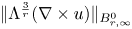
3.2 Global bounds for $\|w\|_{L^{r}}$ and $\|\theta \|_{L^{\infty }}$ and global time integrability $\|\Lambda ^{\frac 3r} (\nabla \times u)\|_{B_{r,\infty }^{0}}$


The major result of this subsection is the global bound stated in the following proposition.
Proposition 3.4 Assume that  $(v, w, \theta )$ solves (1.6) with
 $\eta =0$. Then for any
 $t>0$,
 \begin{align} &\int_0^{t} \|\Lambda^{\frac{3}{r}} (\nabla\times u)(\tau)\|_{B_{r,\infty}^{0}}\,\textrm{d}\tau <\infty, \quad for\ any\ \frac{3}{2\alpha-2}< r<\infty, \end{align}
 \begin{align} &\int_0^{t} \|\nabla u(\tau)\|_{L^{r}}\,\textrm{d}\tau <\infty,\ \|w\|_{L^{r}} <\infty,\quad for\ any\ 2\leq r<\infty, \end{align}
 \begin{align} &\|\theta(t)\|_{L^{r}} <\infty,\quad for\ any\ 2\leq r\leq\infty. \end{align}
Proof. Taking the curl to the first equation of (1.6), we obtain
 \begin{equation} \partial_t \Omega + (\mu +\chi) (-\Delta)^{\alpha} \Omega = 2 \chi \nabla \times(\nabla \times w) + \nabla \times(\theta \mathbf{e}_3) - \nabla \times(u \cdot \nabla u) \end{equation}
with  $\Omega =\nabla \times u$. Next, we write the equation of (3.12) in the integral form
 \begin{align} \Omega(t) &= \textrm{e}^{-(\mu +\chi)(-\Delta)^{\alpha} t} \Omega_0 + 2 \chi \int_0^{t}\,\textrm{e}^{-(\mu+\chi)(-\Delta)^{\alpha} (t-\tau)} \nabla \times(\nabla \times w(\tau))\,\textrm{d}\tau\nonumber\\ &\quad+\int_0^{t}\,\textrm{e}^{-(\mu+\chi)(-\Delta)^{\alpha} (t-\tau)}\nabla \times(\theta(\tau) \mathbf{e}_3)\,\textrm{d}\tau\notag\\ &\quad + \int_0^{t}\,\textrm{e}^{-(\mu+\chi)(-\Delta)^{\alpha} (t-\tau)}\nabla\times\nabla\cdot (u\otimes u)(\tau)\,\textrm{d}\tau. \end{align}
Localizing (3.13) by applying  $\Delta _j$ with
 $j\geq -1$, taking the
 $L^{r}$-norm with
 $r\in [2,\infty )$ and applying lemma A.5 and Bernstein's inequality, we derive that
 \begin{align} \|\Delta_j \Omega(t)\|_{L^{r}} &\leq C\,\textrm{e}^{{-}c_0 (\mu +\chi) t\, 2^{2\alpha j}}\, \|\Delta_j \Omega_0\|_{L^{r}}\notag\\ &\quad + C \, \int_0^{t} 2^{2j}\,\textrm{e}^{{-}c_0 (\mu +\chi) (t-\tau)\, 2^{2\alpha j}} \|\Delta_j w(\tau)\|_{L^{r}}\,\textrm{d}\tau \nonumber\\ &\quad+ C\,\int_0^{t} 2^{j}\,\textrm{e}^{{-}c_0 (\mu +\chi) (t-\tau)\,2^{2\alpha j}} \|\Delta_j \theta(\tau)\|_{L^{r}}\,\textrm{d}\tau\nonumber\\ &\quad+ C\,\int_0^{t} 2^{2j}\,\textrm{e}^{{-}c_0 (\mu +\chi) (t-\tau)\,2^{2\alpha j}} \|\Delta_j (u\otimes u)(\tau)\|_{L^{r}}\,\textrm{d}\tau. \end{align}
To further improve the estimates, we dot the second and third equations in (1.6) with  $w |w|^{r-2}$ and
 $\theta |\theta |^{r-2}$, respectively, and integrate the result in space domain to obtain
 \begin{align*} \frac{1}{r}\frac{\textrm{d}}{\textrm{d}t}\|w\|_{L^{r}}&\leq 2 \chi \int \Omega \cdot w |w|^{r-2},\\ \frac{1}{r}\frac{\textrm{d}}{\textrm{d}t}\|\theta\|_{L^{r}}&\leq\int (u\cdot\mathbf{e}_3) \theta |\theta|^{r-2}, \end{align*}
which yield
 \begin{align} \|w\|_{L^{r}} &\leq \|w_0\|_{L^{r}} + 2 \chi \int_0^{t} \|\Omega(\tau)\|_{L^{r}}\,\textrm{d}\tau, \end{align}
 \begin{align} \|\theta\|_{L^{r}} &\leq \|\theta_0\|_{L^{r}} + \int_0^{t} \|u(\tau)\|_{L^{r}}\,\textrm{d}\tau. \end{align}
By Sobolev's inequality,
 \begin{align} \|u\|_{L^{r}} &\leq C\, \|u\|_{H^{2\alpha-1}}, \end{align}
 \begin{align} \|\Delta_j(u\otimes u)(\tau)\|_{L^{r}} &\leq \|u\|_{L^{2r}}^{2} \leq C\, \|u\|_{H^{2\alpha-1}}^{2}. \end{align}
Note that  $\|\Delta _j w\|_{L^{r}} \leq \|w\|_{L^{r}}$, then combining (3.14) and (3.15)–(3.18), we derive that
 \begin{align} \|\Delta_j \Omega(t)\|_{L^{r}} &\leq C\,\textrm{e}^{{-}c_0 (\mu +\chi) t\, 2^{2\alpha j}}\, \|\Delta_j \Omega_0\|_{L^{r}}\nonumber\\ &\quad+ C\,\int_0^{t} 2^{2j}\,\textrm{e}^{{-}c_0 (\mu +\chi) (t-\tau)\,2^{2\alpha j}} \left(\|w_0\|_{L^{r}} + \int_0^{\tau} \|\Omega(s)\|_{L^{r}}\,\textrm{d}s\right)\,\textrm{d}\tau\nonumber\\ &\quad+C\,\int_0^{t} 2^{j}\,\textrm{e}^{{-}c_0 (\mu +\chi) (t-\tau)\,2^{2\alpha j}} \left(\|\theta_0\|_{L^{r}} + \int_0^{\tau} \|u(s)\|_{H^{2\alpha-1}}\,\textrm{d}s\right)\,\textrm{d}\tau\nonumber\\ &\quad+C\,\int_0^{t} 2^{2j}\,\textrm{e}^{{-}c_0 (\mu +\chi) (t-\tau)\, 2^{2\alpha j}} \|u(\tau)\|_{H^{2\alpha-1}}^{2}\,\textrm{d}\tau. \end{align}
Integrating (3.19) in time and applying Young's inequality for the time convolution, we obtain
 \begin{align} 2^{(2\alpha-2) j}\,\int_0^{t} \|\Delta_j \Omega (\tau)\|_{L^{r}}\,\textrm{d}\tau & \leq C 2^{{-}2j} \|\Delta_j \Omega_0\|_{L^{r}}\notag\\ &\quad + C \int_0^{t} \left(\|w_0\|_{L^{r}} + \int_0^{\tau} \|\Omega(s)\|_{L^{r}}\,\textrm{d}s\right)\,\textrm{d}\tau \nonumber\\ &\quad+C\, \int_0^{t} \left(\|\theta_0\|_{L^{r}} + \int_0^{\tau} \|u(s)\|_{H^{2\alpha-1}}\,\textrm{d}s\right)\,\textrm{d}\tau\nonumber\\ &\quad+C \int_0^{t} \|u(\tau)\|_{H^{2\alpha-1}}^{2}\,\textrm{d}\tau\nonumber\\ &\leq C + C \int_0^{t} \int_0^{\tau} \|\Omega(s)\|_{L^{r}}\,\textrm{d}s\,\textrm{d}\tau, \end{align}
where we have used (3.3) with  $\rho =\alpha -1$ in the last inequality.
Noting that
 \begin{align*} \|\Omega\|_{L^{r}} &\leq \sum_{j\geq{-}1} \|\Delta_j \Omega\|_{L^{r}} \leq \sum_{j\geq{-}1} 2^{(2-2\alpha)j} \, 2^{(2\alpha-2)j}\,\|\Delta_j \Omega\|_{L^{r}}\\ &\leq \sup_{j\geq{-}1} 2^{(2\alpha-2)j}\,\|\Delta_j \Omega\|_{L^{r}},\end{align*}
then (3.20), together with Gronwall's inequality, yields
 \begin{equation} \sup_{j\geq{-}1} 2^{(2\alpha-2) j} \int_0^{t} \|\Delta_j \Omega\|_{L^{r}}\,\textrm{d}\tau <\infty. \end{equation}
Thus this implies for  $r>\frac {3}{2\alpha -2}$,
 \begin{align} \int_0^{t} \|\Lambda^{\frac{3}{r}} \Omega(\tau)\|_{B_{r,\infty}^{0}}\,\textrm{d}\tau&\leq C\int_0^{t} \|\Omega(\tau)\|_{B^{\frac{3}{r}}_{r,1}}\,\textrm{d}\tau\nonumber\\ &= C\int_0^{t} \sum_{j\geq{-}1} 2^{\frac{3}{r}j} \|\Delta_j \Omega(\tau)\|_{L^{r}}\,\textrm{d}\tau \nonumber\\ &\leq C\int_0^{t} \sum_{j\geq{-}1} 2^{(\frac 3r - (2\alpha-2))j} 2^{(2\alpha-2) j} \|\Delta_j \Omega(\tau)\|_{L^{r}}\,\textrm{d}\tau \nonumber\\ &= C\sum_{j\geq{-}1} 2^{(\frac{3}{r} - (2\alpha-2))j} 2^{(2\alpha-2) j} \int_0^{t} \|\Delta_j \Omega(\tau)\|_{L^{r}}\,\textrm{d}\tau\nonumber\\ &\leq C\sup_{j\geq{-}1} 2^{(2\alpha-2) j} \int_0^{t} \|\Delta_j \Omega(\tau)\|_{L^{r}}\,\textrm{d}\tau \sum_{j\geq{-}1} 2^{(\frac{3}{r}- (2\alpha-2))j}\nonumber\\ &= C \sup_{j\geq{-}1} 2^{(2\alpha-2) j} \int_0^{t} \|\Delta_j \Omega(\tau)\|_{L^{r}}\,\textrm{d}\tau <\infty, \end{align}
which leads to (3.9). Furthermore, (3.22), (3.15) and (3.16), together with Gagliardo-Nirenberg's inequality, imply (3.10) and (3.11). Thus the proof of proposition 3.4 is completed.
3.3 Global $H^{s}$ bound

This subsection completes the proof of proposition 3.1 by establishing the global  $H^{s}$ bound.
Proof of proposition 3.1. Applying  $\Lambda ^{s}$ to the first three equations in (1.6), and taking the
 $L^{2}$-inner product to the resulting equations with
 $\Lambda ^{s} u$,
 $\Lambda ^{s} w$ and
 $\Lambda ^{s} \theta$, respectively, we have
 \begin{align} &\frac{1}{2}\frac{\textrm{d}}{\textrm{d}t} (\|\Lambda^{s} u\|_{L^{2}}^{2} + \|\Lambda^{s} w\|_{L^{2}}^{2} + \|\Lambda^{s} \theta\|_{L^{2}}^{2}) + (\mu + \chi) \|\Lambda^{s+\alpha} u\|_{L^{2}}^{2}\nonumber\\ &\quad\leq \int \Lambda^{s} (\theta \mathbf{e}_3)\cdot \Lambda^{s} u - \int [\Lambda^{s}, u\cdot\nabla] u \cdot \Lambda^{s} u + 4\chi \int \Lambda^{s} (\nabla\times u)\cdot \Lambda^{s} w\nonumber\\ &\qquad- \int [\Lambda^{s}, u\cdot\nabla] w \cdot \Lambda^{s} w + \int \Lambda^{s} (u\cdot\mathbf{e}_3)\cdot \Lambda^{s} \theta - \int [\Lambda^{s}, u\cdot\nabla] \theta \cdot \Lambda^{s} \theta\nonumber\\ &\quad:= K_1 + K_2 + K_3 + K_4 + K_5 + K_6. \end{align}
The terms on the right-hand side can be estimated as follows. Using the Young inequality,
 \[ K_1 + K_5\leq \|\Lambda^{s} u\|_{L^{2}}^{2} + \|\Lambda^{s} \theta\|_{L^{2}}^{2}. \]
By commutator estimate lemma A.3,
 \[ K_2 \leq C\,\|\nabla u\|_{L^{\infty}}\,\|\Lambda^{s} u\|_{L^{2}}^{2}. \]
Resorting to Hölder's inequality and Gagliardo-Nirenberg's inequality,
 \begin{align*} K_3&\leq C \|\Lambda^{s+1} u\|_{L^{2}} \|\Lambda^{s} w\|_{L^{2}}\nonumber\\ &\leq C \|u\|_{L^{2}}^{1-\frac{s+1}{s+\alpha}} \|\Lambda^{s+\alpha} u\|_{L^{2}}^{\frac{s+1}{s+\alpha}} \|\Lambda^{s} w\|_{L^{2}}\nonumber\\ &\leq \frac{\mu + \chi}{8} \|\Lambda^{s+\alpha} u\|_{L^{2}}^{2} + C (\|u\|_{L^{2}}^{2} + \|\Lambda^{s} w\|_{L^{2}}^{2}). \end{align*}
Again applying lemma A.3,
 \begin{align*} K_4 &\leq C (\|\Lambda^{s + 1} u\|_{L^{\frac{6}{5 - 2\alpha}}} \|w\|_{L^{\frac{3}{\alpha-1}}} + \|\nabla u\|_{L^{\infty}} \|\Lambda^{s} w\|_{L^{2}}) \|\Lambda^{s} w\|_{L^{2}}\nonumber\\ &\leq C\|\Lambda^{s + \alpha} u\|_{L^{2}} \|w\|_{L^{\frac{3}{\alpha-1}}} \|\Lambda^{s} w\|_{L^{2}} + C\|\nabla u\|_{L^{\infty}} \|\Lambda^{s} w\|_{L^{2}}^{2}\nonumber\\ &\leq \frac{\mu + \chi}{8} \|\Lambda^{s+\alpha} u\|_{L^{2}}^{2} + C \|w\|_{L^{\frac{3}{\alpha-1}}}^{2} \|\Lambda^{s} w\|_{L^{2}}^{2} + C\|\nabla u\|_{L^{\infty}} \|\Lambda^{s} w\|_{L^{2}}^{2}. \end{align*}
Similarly, we have
 \[ K_6 \leq \frac{\mu + \chi}{8} \|\Lambda^{s+\alpha} u\|_{L^{2}}^{2} + C \|\theta\|_{L^{\frac{3}{\alpha-1}}}^{2} \|\Lambda^{s} \theta\|_{L^{2}}^{2} + C\|\nabla u\|_{L^{\infty}} \|\Lambda^{s} \theta\|_{L^{2}}^{2}. \]
Inserting the bounds above in (3.23), we have
 \begin{align} &\frac{\textrm{d}}{\textrm{d}t} (\|\Lambda^{s} u\|_{L^{2}}^{2} + \|\Lambda^{s} w\|_{L^{2}}^{2} + \|\Lambda^{s} \theta\|_{L^{2}}^{2}) + (\mu + \chi) \|\Lambda^{s+\alpha} u\|_{L^{2}}^{2}\nonumber\\ &\quad\leq C\|u\|_{L^{2}}^{2} + C (1 + \|\nabla u\|_{L^{\infty}} + \|w\|_{L^{\frac{3}{\alpha-1}}}^{2} + \|\theta\|_{L^{\frac{3}{\alpha-1}}}^{2}) (\|\Lambda^{s} v\|_{L^{2}}^{2} + \|\Lambda^{s} w\|_{L^{2}}^{2})\nonumber\\ &\quad\leq C + C \left(1 + \|\Lambda^{\frac{3}{r}} (\nabla\times u)\|_{B_{r, \infty}^{0}} \log (e+ \|\Lambda^{s} u\|_{L^{2}})\right)\notag\\ &\quad \times (\|\Lambda^{s} u\|_{L^{2}}^{2} + \|\Lambda^{s} w\|_{L^{2}}^{2} + \|\Lambda^{s} \theta\|_{L^{2}}^{2}), \end{align}
where  $r>\frac {3}{2\alpha -2}$, and we have used (3.1), (3.10), (3.11) and lemma A.6 in the last inequality. Applying Osgood's inequality to (3.24), together with (3.9), we obtain the desired global
 $H^{s}$-bound. This completes the proof of proposition 3.1.
4. Proof of theorem 1.4
This section proves theorem 1.4. Again we prove the global a priori bounds in  $H^{s}$. More precisely, we prove the following proposition.
Proposition 4.1 Consider (1.6) with  $\mu >0$,
 $\chi >0$,
 $\eta >0$ and
 $\alpha \geq \frac {7}{4}$. Assume
 $(u_0, w_0, \theta _0)\in H^{s}(\mathbb {R}^{3})$ with
 $s>\frac {5}{2}$ and
 $\nabla \cdot u_0=0$. Then the corresponding solution
 $(u, w, \theta )$ of (1.6) is globally bounded in
 $H^{s}(\mathbb {R}^{3})$.
The proof of proposition 4.1 is partially similar as that of proposition 3.1. Here we sketch the proof and point out the main differences.
Proof of proposition 4.1. Similar as the proof of (3.1) and (3.3), we obtain for any  $t>0$,
 \begin{equation} \|u\|_{L^{2}}^{2} + \|w\|_{L^{2}}^{2} + \|\theta\|_{L^{2}}^{2} +\int_0^{t}\|\Lambda^{\alpha} u(\tau)\|_{L^{2}}^{2}\,\textrm{d}\tau \leq C, \end{equation}
and
 \begin{equation} \|\Lambda^{\rho} u\|_{L^{2}}^{2} + \int_0^{t} \|\Lambda^{\rho+\alpha} u(\tau)\|_{L^{2}}^{2}\,\textrm{d}\tau\leq C, \end{equation}
for  $0<\rho \leq \alpha -1$. Choosing
 $\rho =\alpha -1$, then (4.1)–(4.2) together with the Gagliardo-Nirenberg inequality imply
 \begin{equation} \int_0^{t} \|\Lambda^{\frac{5}{2}} u(\tau)\|_{L^{2}}^{2}\,\textrm{d}\tau\leq C \int_0^{t} (\|u(\tau)\|_{L^{2}}^{2} + \|\Lambda^{2\alpha-1} u(\tau)\|_{L^{2}}^{2})\,\textrm{d}\tau <\infty. \end{equation}
This immediately yields
 \begin{equation} \int_0^{t} \|\Lambda^{\frac{3}{2}} (\nabla\times u)(\tau)\|_{B_{2,\infty}^{0}}\,\textrm{d}\tau \leq C\int_0^{t} \|\Lambda^{\frac{5}{2}} u(\tau)\|_{L^{2}}\,\textrm{d}\tau <\infty. \end{equation}
Furthermore, (4.3) together with (3.16) yields for any  $2\leq r\leq \infty$,
 \begin{equation} \|\theta(t)\|_{L^{r}} <\infty. \end{equation}
In the following, to bound  $\|w(t)\|_{L^{r}}$, we apply
 $\Lambda ^{\frac {3}{2}}$ to the first three equations in (1.6), take the
 $L^{2}$-inner product to the result with
 $\Lambda ^{\frac {3}{2}} u$,
 $\Lambda ^{\frac {3}{2}} w$ and
 $\Lambda ^{\frac {3}{2}} \theta$, respectively, and add them up to obtain
 \begin{align} &\frac{1}{2}\frac{\textrm{d}}{\textrm{d}t} (\|\Lambda^{\frac{3}{2}} u\|_{L^{2}}^{2} + \|\Lambda^{\frac{3}{2}} w + \|\Lambda^{\frac{3}{2}} \theta\|_{L^{2}}^{2}) + (\mu + \chi) \|\Lambda^{\frac{3}{2}+\alpha} u\|_{L^{2}}^{2}\notag\\ &\quad + 4\chi \|\Lambda^{\frac{3}{2}} w\|_{L^{2}}^{2} + \eta\|\Lambda^{\frac{3}{2}} \nabla\cdot w\|_{L^{2}}^{2}\nonumber\\ &\quad=\int \Lambda^{\frac{3}{2}} (\theta \mathbf{e}_3)\cdot \Lambda^{\frac{3}{2}} u - \int [\Lambda^{\frac{3}{2}}, u\cdot\nabla] u \cdot \Lambda^{\frac{3}{2}} u + 4\chi \int \Lambda^{\frac{3}{2}} \nabla\times u\cdot \Lambda^{\frac{3}{2}} w\nonumber\\ &\qquad- \int [\Lambda^{\frac{3}{2}}, u\cdot \nabla] w \cdot \Lambda^{\frac{3}{2}} w + \int \Lambda^{\frac{3}{2}} (u\cdot\mathbf{e}_3)\cdot \Lambda^{\frac{3}{2}} \theta - \int [\Lambda^{\frac{3}{2}}, u\cdot\nabla] \theta \cdot \Lambda^{\frac{3}{2}} \theta\nonumber\\ &\quad:= J_1 + J_2 + J_3 + J_4 + J_5 + J_6. \end{align}
Applying the Young inequality,
 \begin{equation} J_1 + J_5\leq \|\Lambda^{\frac{3}{2}} u\|_{L^{2}}^{2} + \|\Lambda^{\frac{3}{2}} \theta\|_{L^{2}}^{2}. \end{equation}
By commutator estimate lemma A.3,
 \begin{equation} J_2 \leq C\,\|\nabla u\|_{L^{\infty}}\,\|\Lambda^{\frac{3}{2}} u\|_{L^{2}}^{2}. \end{equation}
Using Hölder's inequality and the Young inequality,
 \begin{align} J_3&\leq C \|\Lambda^{\frac{5}{2}} u\|_{L^{2}} \|\Lambda^{\frac{3}{2}} w\|_{L^{2}}\nonumber\\ &\leq C (\|u\|_{L^{2}} + \|\Lambda^{\frac{3}{2}+\alpha} u\|_{L^{2}}) \|\Lambda^{\frac{3}{2}} w\|_{L^{2}}\nonumber\\ &\leq \frac{\mu + \chi}{2} \|\Lambda^{\frac{3}{2}+\alpha} u\|_{L^{2}}^{2} + C (\|u\|_{L^{2}}^{2} + \|\Lambda^{\frac{3}{2}} w\|_{L^{2}}^{2}). \end{align}
Applying commutator estimate lemma A.3 and Sobolev's imbedding, we infer that
 \begin{align} J_4&\leq \|[\Lambda^{\frac{3}{2}}, u\cdot \nabla] w\|_{L^{2}} \|\Lambda^{\frac{3}{2}} w\|_{L^{2}}\nonumber\\ &\leq C (\|\Lambda^{\frac{3}{2}} u\|_{L^{6}} \|\nabla w\|_{L^{3}} + \|\nabla u\|_{L^{\infty}} \|\Lambda^{\frac{3}{2}} w\|_{L^{2}} )\|\Lambda^{\frac{3}{2}} w\|_{L^{2}}\nonumber\\ &\leq C (\|\Lambda^{\frac{5}{2}} u\|_{L^{2}} + \|\nabla u\|_{L^{\infty}})\|\Lambda^{\frac{3}{2}} w\|_{L^{2}}^{2}. \end{align}
Similarly, we have
 \begin{equation} J_6\leq C (\|\Lambda^{\frac{5}{2}} u\|_{L^{2}} + \|\nabla u\|_{L^{\infty}})\|\Lambda^{\frac{3}{2}} \theta\|_{L^{2}}^{2}. \end{equation}
Substituting (4.7)–(4.11) into (4.6), we obtain
 \begin{align} &\frac{\textrm{d}}{\textrm{d}t} \left(\|\Lambda^{\frac{3}{2}} u\|_{L^{2}}^{2} + \|\Lambda^{\frac{3}{2}} w + \|\Lambda^{\frac{3}{2}} \theta\|_{L^{2}}^{2}\right) + (\mu + \chi) \|\Lambda^{\frac{3}{2}+\alpha} u\|_{L^{2}}^{2}\nonumber\\ &\quad\leq C \|u\|_{L^{2}}^{2} + C \left(1+ \|\Lambda^{\frac{5}{2}} u\|_{L^{2}} + \|\nabla u\|_{L^{\infty}}\right) \left(\|\Lambda^{\frac{3}{2}} u\|_{L^{2}}^{2} + \|\Lambda^{\frac{3}{2}} w + \|\Lambda^{\frac{3}{2}} \theta\|_{L^{2}}^{2}\right)\nonumber\\ &\quad\leq C \,{+}\, C \left(1\,{+}\, \|\Lambda^{\frac{5}{2}} u\|_{L^{2}}\log \left(e+ \|\Lambda^{\frac{3}{2}+\alpha} u\|_{L^{2}}\right)\right) \left(\|\Lambda^{\frac{3}{2}} u\|_{L^{2}}^{2} + \|\Lambda^{\frac{3}{2}} w + \|\Lambda^{\frac{3}{2}} \theta\|_{L^{2}}^{2}\right), \end{align}
where we have used (4.1), lemma A.6 and the fact  $\|\Lambda ^{\frac {3}{2}} (\nabla \times u)\|_{B_{2, \infty }^{0}}\leq C \|\Lambda ^{\frac {5}{2}} u\|_{L^{2}}$ in the last inequality. Then (4.12), together with lemma A.7, yields
 \begin{equation} \|\Lambda^{\frac{3}{2}} u\|_{L^{2}}^{2} + \|\Lambda^{\frac{3}{2}} w\|_{L^{2}}^{2} + \|\Lambda^{\frac{3}{2}} \theta\|_{L^{2}}^{2} + \int_0^{t}\|\Lambda^{\frac{3}{2}+\alpha} u(\tau)\|_{L^{2}}^{2}\,\textrm{d}\tau\leq C. \end{equation}
In particular, this together with (4.1) implies for any  $2\leq r<\infty$,
 \begin{equation} \|w(t)\|_{L^{r}} <\infty. \end{equation}
With these bounds at our disposal, similar as the derivation of (3.24), together with (4.5) and (4.14), we obtain
 \begin{align} &\frac{\textrm{d}}{\textrm{d}t} (\|\Lambda^{s} u\|_{L^{2}}^{2} + \|\Lambda^{s} w\|_{L^{2}}^{2} + \|\Lambda^{s} \theta\|_{L^{2}}^{2}) + (\mu + \chi) \|\Lambda^{s+\alpha} u\|_{L^{2}}^{2}\nonumber\\ &\quad\leq C + C \left(1 + \|\Lambda^{\frac{3}{2}} (\nabla\times u)\|_{B_{2,\infty}^{0}} \log (e+ \|\Lambda^{s} u\|_{L^{2}})\right)\notag\\ &\qquad \times (\|\Lambda^{s} u\|_{L^{2}}^{2} + \|\Lambda^{s} w\|_{L^{2}}^{2} + \|\Lambda^{s} \theta\|_{L^{2}}^{2}). \end{align}
Applying Osgood's inequality to (4.15), together with (4.4), we obtain the desired global  $H^{s}$-bound. This completes the proof of proposition 4.1.
Appendix A. Functional spaces and inequalities
Appendix A.1 Functional spaces
This subsection provides the definition of the Littlewood-Paley decomposition and the definition of Besov spaces. Some related facts used in the previous sections are also included. Materials presented in this appendix can be found in several books and many papers (see, e.g., [Reference Bahouri, Chemin and Danchin3, Reference Bergh and Löfström4, Reference Miao, Wu and Zhang37, Reference Runst and Sickel40, Reference Triebel49]).
We start with several notation.  $\mathcal {S}$ denotes the usual Schwarz class and
 ${\mathcal {S}}'$ its dual, the space of tempered distributions. Let
 $d\geq 2$. To introduce the Littlewood-Paley decomposition, we write for each
 $j\in \mathbb {Z}$
 \[ A_j =\left\{ \xi \in \mathbb{R}^{d}:\ 2^{j-1} \le |\xi| <2^{j+1}\right\}. \]
The Littlewood-Paley decomposition asserts the existence of a sequence of functions 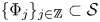 $\{\Phi _j\}_{j\in \mathbb {Z}}\subset {\mathcal {S}}$ such that
 \[ \text{supp} \widehat{\Phi}_j \subset A_j, \quad\widehat{\Phi}_j(\xi) = \widehat{\Phi}_0(2^{{-}j} \xi) \quad\text{or}\quad \Phi_j (x) =2^{jd} \Phi_0(2^{j} x), \]
and
 \[ \sum_{j={-}\infty}^{\infty} \widehat{\Phi}_j(\xi) = \left\{\begin{array}{@{}ll} 1, & \text{if}\ \xi\in \mathbb{R}^{d}\setminus \{0\},\\ 0, & \text{if}\ \xi=0. \end{array} \right. \]
Therefore, for a general function  $\psi \in {\mathcal {S}}$, we have
 \[ \sum_{j={-}\infty}^{\infty} \widehat{\Phi}_j(\xi) \widehat{\psi}(\xi)=\widehat{\psi}(\xi) \quad\text{for} \xi\in \mathbb{R}^{d}\setminus \{0\}. \]
We now choose  $\Psi \in {\mathcal {S}}$ such that
 \[ \widehat{\Psi} (\xi) = 1 - \sum_{j=0}^{\infty} \widehat{\Phi}_j (\xi),\quad \xi \in \mathbb{R}^{d}. \]
Then, for any  $\psi \in {\mathcal {S}}$,
 \[ \Psi \ast \psi + \sum_{j=0}^{\infty} \Phi_j \ast \psi =\psi \]
and hence
 \begin{equation} \Psi \ast f + \sum_{j=0}^{\infty} \Phi_j \ast f =f \end{equation}
in  ${\mathcal {S}}'$ for any
 $f\in {\mathcal {S}}'$. To define the inhomogeneous Besov space, we set
 \begin{equation} \Delta_j f = \left\{\begin{array}{@{}ll} 0, & \text{if}\ j\le -2, \\ \Psi\ast f, & \text{if}\ j={-}1, \\ \Phi_j \ast f, & \text{if}\ j=0,1,2,\cdots. \end{array}\right. \end{equation}
Definition A.1 The inhomogeneous Besov space  $B^{s}_{p,q}$ with
 $s\in \mathbb {R}$ and
 $p,q \in [1,\infty ]$ consists of
 $f\in {\mathcal {S}}'$ satisfying
 \[ \|f\|_{B^{s}_{p,q}(\mathbb{R}^{d})} \equiv \|2^{js} \|\Delta_j f\|_{L^{p}(\mathbb{R}^{d})} \|_{l^{q}}<\infty, \]
where  $\Delta _j f$ is as defined in (A.2).
Bernstein's inequalities are useful tools in dealing with Fourier localized functions. These inequalities trade integrability for derivatives. The following proposition provides Bernstein type inequalities for fractional derivatives. The upper bounds also hold when the fractional operators are replaced by partial derivatives.
Proposition A.2 Let  $\alpha \ge 0$ and
 $1\le p\le q\le \infty$.
(1) If
$f$ satisfies
for some integer\[ \text{supp}\, \widehat{f} \subset \{\xi\in \mathbb{R}^{d}:\ |\xi|\le K 2^{j} \}, \]$j$ and a constant $K>0$, then
\[ \|(-\Delta)^{\alpha} f\|_{L^{q}(\mathbb{R}^{d})} \le C_1\, 2^{2\alpha j +j d\left(\frac{1}{p}-\frac{1}{q}\right)} \|f\|_{L^{p}(\mathbb{R}^{d})}. \](2) If
$f$ satisfies
for some integer\[ \text{supp}\, \widehat{f} \subset \{\xi\in \mathbb{R}^{d}:\ K_12^{j}\le |\xi| \le K_2 2^{j} \} \]$j$ and constants $0< K_1\le K_2$, then
where\[ C_1\, 2^{2\alpha j} \|f\|_{L^{q}(\mathbb{R}^{d})} \le \|(-\Delta)^{\alpha} f\|_{L^{q}(\mathbb{R}^{d})} \le C_2\, 2^{2\alpha j + j d\left(\frac{1}{p}-\frac{1}{q}\right)} \|f\|_{L^{p}(\mathbb{R}^{d})}, \]$C_1$ and $C_2$ are constants depending on $\alpha ,p$ and $q$.


Appendix A.2 Inequalities
This subsection provides several calculus inequalities and logarithmic interpolation inequalities involving fractional Laplacian operators. The first contains two commutator estimates, which are stated in the following two lemmas. They can be found in [Reference Kato and Ponce29, Reference Kenig, Ponce and Vega30] and [Reference Shang41], respectively. We recall that  $\Lambda =(-\Delta )^{\frac 12}$ denotes the Zygmund operator.
Lemma A.3 Let  $s>0$ and
 $d\geq 2$. Let
 $1< r<\infty$ and
 $\frac {1}{r}=\frac {1}{p_1}+\frac {1}{q_1}=\frac {1}{p_2}+\frac {1}{q_2}$ with
 $q_1, p_2\in (1,\infty )$ and
 $p_1, q_2\in [1,\infty ]$. Then,
 \[ \|[\Lambda^{s},f ]g \|_{L^{r}(\mathbb{R}^{d})}\leq C\left(\|\nabla f \|_{L^{p_1}(\mathbb{R}^{d})}\|\Lambda^{s-1} g \|_{L^{q_1}(\mathbb{R}^{d})} + \|\Lambda^{s} f \|_{L^{p_2}(\mathbb{R}^{d})} \| g \|_{L^{q_2}(\mathbb{R}^{d})}\right) \]
and
 \[ \|\Lambda^{s}(f\,g)\|_{L^{r}(\mathbb{R}^{d})} \le C\, \left(\|\Lambda^{s} f\|_{L^{p_1}(\mathbb{R}^{d})}\, \| g\|_{L^{q_1}(\mathbb{R}^{d})} + \|f\|_{L^{p_2}(\mathbb{R}^{d})}\,\|\Lambda^{s} g\|_{L^{q_2}(\mathbb{R}^{d})}\right), \]
where  $[\Lambda ^{s},f]g = \Lambda ^{s}(fg) - f\Lambda ^{s} g$ and
 $C$'s are constants depending on the indices
 $s, r, p_1, q_1, p_2$ and
 $q_2$.
Lemma A.4 Let  $d\geq 2$,
 $f$ be a smooth divergence free vector field and
 $g$ be a smooth scalar function. Then, for all
 $r>1$ and
 $j\geq -1$,
 \[ \|[\Delta_j, f\cdot\nabla] g\|_{L^{r}(\mathbb{R}^{d})}\leq C\, \|\nabla f\|_{L^{r}(\mathbb{R}^{d})} \|g\|_{L^{\infty}(\mathbb{R}^{d})}. \]
The second tool provides an upper bound for the action of the generalized heat operator on functions with Fourier transform supported on an annulus. The bound for the standard heat operator can be found in [Reference Bahouri, Chemin and Danchin3]. This generalization can be established by modifying the original proof.
Lemma A.5 Let  $\mathcal {A}=\{\xi \in \mathbb {R}^{d}: r_1\le |\xi |\le r_2\}$ with
 $d\geq 2$ and
 $0< r_1< r_2$ being constants. Let
 $\alpha >0$. Then, there exist
 $c>0$ and
 $C>0$ such that, for
 $p\in [1,\infty ]$ and
 $f$ satisfying
 \[ f\in L^{p}(\mathbb{R}^{d}),\quad \text{supp} \widehat{f} \subset \lambda \mathcal{A}, \]
we have, for  $t>0$ and
 $\lambda >0$,
 \[ \|\textrm{e}^{-(-\Delta)^{\alpha} t} f\|_{L^{p}(\mathbb{R}^{d})} \le C\, \textrm{e}^{{-}c t \lambda^{2\alpha}}\, \|f\|_{L^{p}(\mathbb{R}^{d})}. \]
The third preparation provides the following logarithmic type Besov interpolation inequalities. The version presented here is a variant of the standard ones and we provide a proof.
Lemma A.6 Let  $s>1+\frac {d}{q}$ with
 $d\geq 2$ and
 $q\in (1, \infty )$. Then for
 $r\in (1, \infty ]$, there exist two constants
 $C_1$ and
 $C_2$ such that
 \begin{align} \|\nabla f\|_{L^{\infty}(\mathbb{R}^{d})} &\leq C_1 (1 + \|f\|_{L^{2}(\mathbb{R}^{d})})\notag\\ &\quad + C_2(\|\Lambda^{\frac{d}{r}}(\nabla\times f)\|_{B_{r,\infty}^{0}(\mathbb{R}^{d})}\, \log (e + \|\Lambda^{s} f\|_{L^{q}(\mathbb{R}^{d})})). \end{align}
Proof. For an integer  $N>1$ to be determined later, we write
 \[ \|\nabla f\|_{L^{\infty}} \leq \|\Delta_{{-}1} \nabla f\|_{L^{\infty}} + \sum_{0\leq j\le N-1} \|\Delta_j \nabla f\|_{L^{\infty}} + \sum_{j\geq N} \|\Delta_j \nabla f\|_{L^{\infty}}. \]
It then follows from Bernstein's inequality that
 \begin{align} \|\nabla f\|_{L^{\infty}} &\leq C \|f\|_{L^{2}} + C \sum_{0\leq j\leq N-1} 2^{\frac{d}{r}j} \|\Delta_j (\nabla\times f)\|_{L^{r}} + C\sum_{j\ge N} 2^{\left(1 + \frac{d}{q}\right)j} \|\Delta_j f\|_{L^{q}}\nonumber\\ &\leq C \|f\|_{L^{2}} + CN \|\Lambda^{\frac{d}{r}}(\nabla\times f)\|_{B_{r,\infty}^{0}} + C \sum_{j\ge N} 2^{\left(1 + \frac{d}{q}-s\right)j} \|\Lambda^{s} \Delta_j f\|_{L^{q}} \nonumber\\ &\leq C \|f\|_{L^{2}} + CN \|\Lambda^{\frac{d}{r}}(\nabla\times f)\|_{B_{r,\infty}^{0}} + C 2^{\left(1 + \frac{d}{q}-s\right)N} \|\Lambda^{s} f\|_{L^{q}}. \end{align}
Since  $s>1 + \frac {d}{2}$, we can take
 $N$ such that
 $2^{\left (1 + \frac {d}{q}-s\right )N} \|\Lambda ^{s} f\|_{L^{2}} \le 1$, namely
 \[ N= 1+ \text{INT}\left[\frac{1}{\left(s-1 -\frac{d}{q}\right)\ln 2} \log (e+ \|\Lambda^{s} f\|_{L^{q}})\right], \]
where  $\text {INT}$ denotes the integer part of a real number. Inserting
 $N$ in (A.4), we obtain (A.3). This completes the proof of lemma A.6.
Finally, we recall the generalizing Osgood type lemma (see, e.g., [Reference Li and Titi32, Reference Shang and Wu43]).
Lemma A.7 Assume that  $Y,Z,A$ and
 $B$ are non-negative functions satisfying
 \[ \frac{{\rm d}}{{\rm d}t} Y(t) + Z(t) \le A(t) \, Y(t) + B(t)\, Y(t)\, \ln(1 + Z(t)), \]
Let  $T>0$. Assume
 $A\in L^{1}(0, T)$ and
 $B\in L^{2}(0,T)$. Then, for any
 $t\in [0,T]$,
 \[ Y(t) \le (1+Y(0))^{\textrm{e}^{\int_0^{t} B(\tau)\,\textrm{d}\tau}}\,\textrm{e}^{\int_0^{t}\,\textrm{e}^{\int_s^{t} B(\tau)\,\textrm{d}\tau}(A(s) + B^{2}(s))\,\textrm{d}s} \]
and
 \[ \int_0^{t} Z(\tau)\,\textrm{d}\tau \le Y(t)\,\int_0^{t} A(\tau)\,\textrm{d}\tau + Y^{2}(t)\, \int_0^{t} B^{2}(\tau)\,\textrm{d}\tau <\infty. \]
Acknowledgments
The authors would like to express their sincere thanks to the anonymous referee for the constructive and insightful comments which significantly improved the manuscript. Shang would like to express his sincere gratitude to Professor Jiahong Wu for his teaching and useful discussions.


