1 Introduction
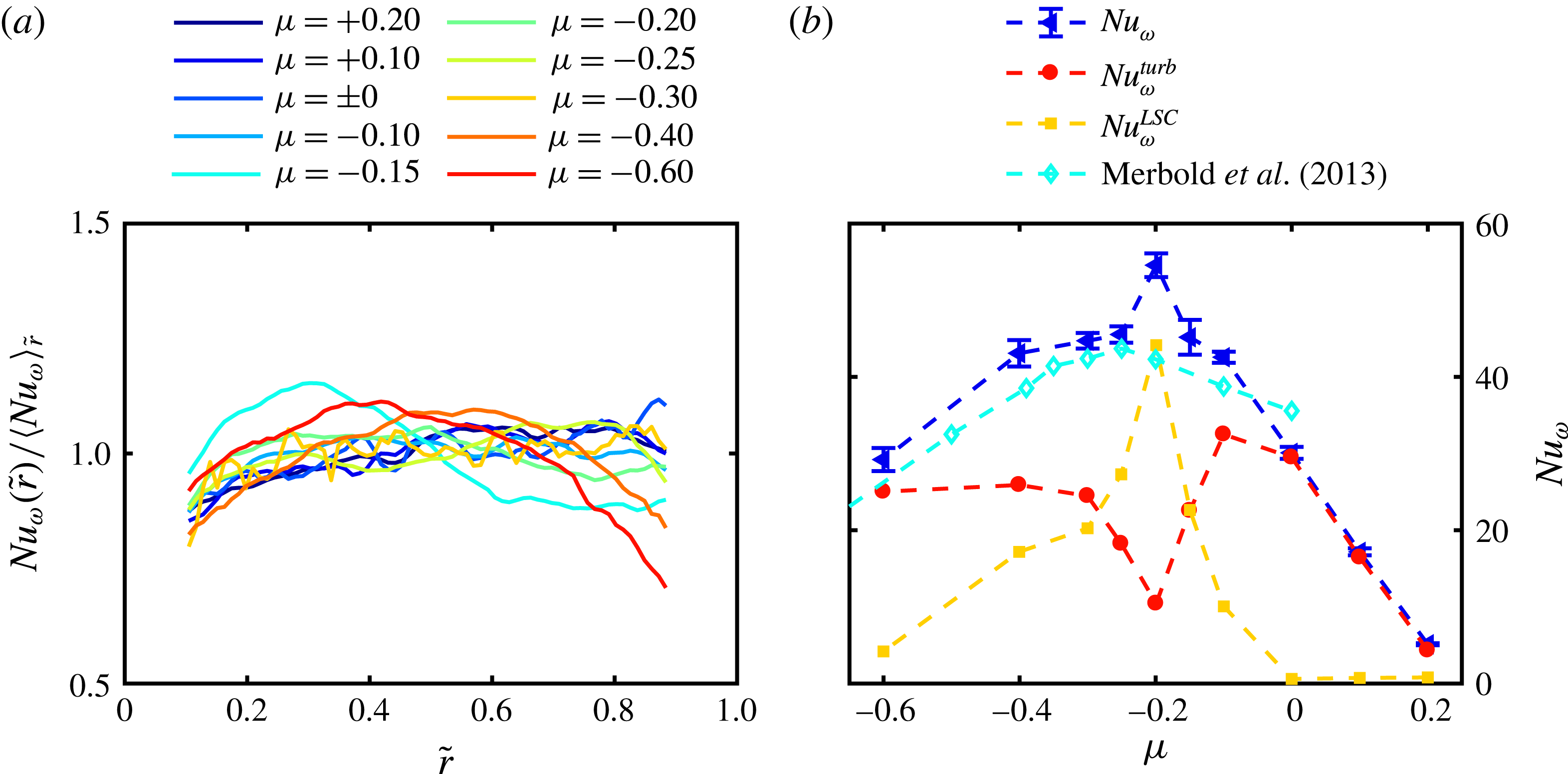
The flow in the gap between two concentric and independently rotating cylinders holds a huge variety of flow states due to hydrodynamic instabilities not only in the laminar and transitional but also in the fully turbulent regime (DiPrima & Swinney Reference Diprima and Swinney1981; Andereck, Liu & Swinney Reference Andereck, Liu and Swinney1986; Dong & Zheng Reference Dong and Zheng2011; van der Veen et al.
Reference van der Veen, Huisman, Merbold, Harlander, Egbers, Lohse and Sun2016). The most famous examples are the centrifugally driven Taylor vortices arising in the laminar flow, which can also survive up to very high Reynolds numbers,
 $Re=O(10^{6})$
(Huisman et al.
Reference Huisman, van der Veen, Sun and Lohse2014). Owing to the plurality of applications, such as astrophysical accretion discs, turbines or journal bearings, the so-called Taylor–Couette (TC) flow has been investigated for over 100 years and is still an active research topic (Donnelly Reference Donnelly1991; Grossmann, Lohse & Sun Reference Grossmann, Lohse and Sun2016). The geometry of the system with an inner (1) and outer (2) cylinder is defined by the radius ratio
 $\unicode[STIX]{x1D702}=r_{1}/r_{2}$
, the gap width
 $d=r_{2}-r_{1}$
and the aspect ratio
 $\unicode[STIX]{x1D6E4}=L/d$
(see figure 1). Further, the rotation rates
 $\unicode[STIX]{x1D714}_{1}$
and
 $\unicode[STIX]{x1D714}_{2}$
of the inner (IC) and outer (OC) cylinders can be represented in dimensionless form by two Reynolds numbers,
 $Re_{1,2}=r_{1,2}\unicode[STIX]{x1D714}_{1,2}d/\unicode[STIX]{x1D708}$
, with
 $\unicode[STIX]{x1D708}$
being the kinematic viscosity of the fluid. In this paper instead of
 $Re_{1,2}$
we use the shear Reynolds number
 $Re_{S}$
, which is an azimuthal Reynolds number measuring the influence of shear and enables comparisons to general rotating shear flows (Dubrulle et al.
Reference Dubrulle, Dauchot, Daviaud, Longaretti, Richard and Zahn2005):
 $$\begin{eqnarray}Re_{S}=\frac{2r_{1}r_{2}d}{(r_{1}+r_{2})\unicode[STIX]{x1D708}}|\unicode[STIX]{x1D714}_{2}-\unicode[STIX]{x1D714}_{1}|=\frac{2}{(1+\unicode[STIX]{x1D702})}|\unicode[STIX]{x1D702}Re_{2}-Re_{1}|\overset{!}{=}\frac{u_{S}d}{\unicode[STIX]{x1D708}}.\end{eqnarray}$$
Based on (1.1) we can introduce a shear velocity
 $u_{S}$
, as a Reynolds number always consists of a characteristic velocity, a characteristic length and the viscosity of the fluid. To define the kinematics of the flow, we use the ratio of angular velocities
 $\unicode[STIX]{x1D707}=\unicode[STIX]{x1D714}_{2}/\unicode[STIX]{x1D714}_{1}$
, which we call the rotation ratio. This parameter offers an intuitive differentiation of flow states, as
 $\unicode[STIX]{x1D707}>0$
means co-rotation,
 $\unicode[STIX]{x1D707}<0$
counter-rotation and
 $\unicode[STIX]{x1D707}=0$
pure inner cylinder rotation.
So far, numerical and experimental studies in wide-gap TC flows, where the radius ratio
 $\unicode[STIX]{x1D702}$
is smaller than 0.7, have been concentrated on mean flow characteristics and turbulent statistics (Bilson & Bremhorst Reference Bilson and Bremhorst2007; Dong Reference Dong2007, Reference Dong2008; van Hout & Katz Reference van Hout and Katz2011), endwall effects (Schartmann et al.
Reference Schartmann, Ji, Burin and Goodman2012; Poncet et al.
Reference Poncet, Viazzo, Aubert, da Soghe and Bianchini2013), bubble dispersion and accumulation (Chouippe et al.
Reference Chouippe, Climent, Legendre and Gabillet2014) and angular momentum transport (Wendt Reference Wendt1933; Merbold, Brauckmann & Egbers Reference Merbold, Brauckmann and Egbers2013; Ostilla-Mónico et al.
Reference Ostilla-Mónico, Huisman, Janninik, van Gils, Verzicco, Grossmann and Lohse2014a
,Reference Ostilla-Mónico, van der Poel, Verzicco, Grossmann and Lohse
b
). Based on the last mentioned topic, we will show why wide-gap TC flows are of particular interest and which flow aspects have to be investigated in more detail. The angular momentum transport is the conserved transport quantity in TC flows and is defined according to Eckhardt, Grossmann & Lohse (so-called EGL theory; see Eckhardt, Grossmann & Lohse (Reference Eckhardt, Grossmann and Lohse2007b
)) as
 $$\begin{eqnarray}J^{\unicode[STIX]{x1D714}}=r^{3}(\langle u_{r}\unicode[STIX]{x1D714}\rangle _{A(r),t}-\unicode[STIX]{x1D708}\unicode[STIX]{x2202}_{r}\langle \unicode[STIX]{x1D714}\rangle _{A(r),t}).\end{eqnarray}$$
The brackets
 $\langle ~\rangle _{A(r),t}$
denote an average over a cylindrical surface at radius
 $r$
and time
 $t$
. At the cylinder walls
 $\langle u_{r}\unicode[STIX]{x1D714}\rangle _{A,t}$
vanishes and
 $J^{\unicode[STIX]{x1D714}}$
can be directly measured by the torque acting on these walls. Using the corresponding laminar value
 $J_{lam}^{\unicode[STIX]{x1D714}}=2\unicode[STIX]{x1D708}r_{1}^{2}r_{2}^{2}(\unicode[STIX]{x1D714}_{1}-\unicode[STIX]{x1D714}_{2})(r_{2}^{2}-r_{1}^{2})$
a quasi-Nusselt number can be defined as a measure for the angular momentum transport:
 $$\begin{eqnarray}Nu_{\unicode[STIX]{x1D714}}=\frac{J^{\unicode[STIX]{x1D714}}}{J_{lam}^{\unicode[STIX]{x1D714}}}.\end{eqnarray}$$
Further, as
 $J^{\unicode[STIX]{x1D714}}$
is independent of the radius, the gradients of the angular velocity at the inner and outer cylinder are connected by the radius ratio
 $\unicode[STIX]{x1D702}$
:
 $$\begin{eqnarray}\unicode[STIX]{x2202}_{r}\langle \unicode[STIX]{x1D714}\rangle _{A(r_{2}),t}=\unicode[STIX]{x1D702}^{3}\unicode[STIX]{x2202}_{r}\langle \unicode[STIX]{x1D714}\rangle _{A(r_{1}),t}.\end{eqnarray}$$
If
 $\unicode[STIX]{x1D702}$
is small, a considerable asymmetry in the wall gradients is present, reflecting the influence of curvature in the system, which suggests a different flow behaviour from narrow-gap TC flows (
 $\unicode[STIX]{x1D702}>0.7$
).
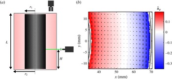
(a) Sketch of the PIV set-up and (b) temporal and axial averaged azimuthal flow field in a horizontal plane at shear Reynolds number
 $Re_{S}=10^{5}$
and rotation ratio
 $\unicode[STIX]{x1D707}=-0.4$
. For the sake of clarity only every fourth velocity vector is shown in both coordinate directions.

In the literature the torque in TC flows for an outer cylinder at rest and differential rotation has been investigated intensively in the past (Paoletti & Lathrop Reference Paoletti and Lathrop2011; van Gils et al.
Reference van Gils, Grossmann, Sun and Lohse2012; Brauckmann & Eckhardt Reference Brauckmann and Eckhardt2013a
; Merbold et al.
Reference Merbold, Brauckmann and Egbers2013), finding a maximum as a function of the radius ratio
 $\unicode[STIX]{x1D702}$
, when the shear Reynolds number is kept constant and only the rotation ratio
 $\unicode[STIX]{x1D707}$
is changed. For
 $\unicode[STIX]{x1D702}=0.5$
it is located in the low counter-rotating regime at
 $\unicode[STIX]{x1D707}_{max}=-0.2$
(Brauckmann & Eckhardt Reference Brauckmann and Eckhardt2013b
; Merbold et al.
Reference Merbold, Brauckmann and Egbers2013; Ostilla-Mónico et al.
Reference Ostilla-Mónico, Huisman, Janninik, van Gils, Verzicco, Grossmann and Lohse2014a
). This maximum is connected to a formation or strengthening of turbulent Taylor vortices, which enhance the momentum transport (Ostilla-Mónico et al.
Reference Ostilla-Mónico, van der Poel, Verzicco, Grossmann and Lohse2014b
; van der Veen et al.
Reference van der Veen, Huisman, Merbold, Harlander, Egbers, Lohse and Sun2016). Brauckmann & Eckhardt (Reference Brauckmann and Eckhardt2013b
) postulated a prediction for this maximum point
 $\unicode[STIX]{x1D707}_{max}(\unicode[STIX]{x1D702})$
based on the work of Esser & Grossmann (Reference Esser and Grossmann1996), which we therefore call the EG prediction. They stated that the turbulent Taylor vortices can extend the theoretical neutral line, where
 $u_{\unicode[STIX]{x1D711}}$
vanishes, into the stable flow region. If this extension reaches the outer cylinder wall, the unstable flow grows most efficient, causing a maximum in torque. This prediction is only valid for
 $\unicode[STIX]{x1D702}\leqslant 0.71$
due to a decreasing stability difference of the inner and outer cylinder regions with increasing radius ratio (Brauckmann, Salewsky & Eckhardt Reference Brauckmann, Salewsky and Eckhardt2016).
However, besides direct torque measurements validating the maximum point, changes in the flow field according to the described prediction have been investigated mainly numerically and at low Reynolds numbers. What is known up to now is that the angular velocity profiles strongly depend on the rotation ratio
 $\unicode[STIX]{x1D707}$
and that the gradient of the profiles becomes small in the low counter-rotating regime. Ostilla-Mónico et al. (Reference Ostilla-Mónico, Huisman, Janninik, van Gils, Verzicco, Grossmann and Lohse2014a
) reported the smallest gradient of angular velocity coinciding with the rotation ratio of the torque maximum for
 $\unicode[STIX]{x1D702}=0.5,0.714,0.833,0.909$
, while Brauckmann et al. (Reference Brauckmann, Salewsky and Eckhardt2016) could validate these results only for
 $\unicode[STIX]{x1D702}\geqslant 0.8$
. This difference may be the result of differences in the investigated
 $Re_{S}$
regime and in the evaluation methods, and measurements at
 $Re_{S}$
far beyond those of Brauckmann et al. (Reference Brauckmann, Salewsky and Eckhardt2016) (
 $Re_{S}=2\times 10^{4}$
) could give more clarity. Further, the radial location of the neutral line is of special interest for the EG prediction. Ostilla et al. (Reference Ostilla, Stevens, Grossmann, Verzicco and Lohse2013) found the detachment of the neutral line from the outer cylinder wall starting at pure inner cylinder rotation for
 $Re_{S}\leqslant 4620$
, while van Gils et al. (Reference van Gils, Grossmann, Sun and Lohse2012) identified a coincidence of
 $\unicode[STIX]{x1D707}_{max}$
with the neutral line detachment for
 $Re_{S}>9\times 10^{5}$
. Both studies were carried out at a radius ratio of
 $\unicode[STIX]{x1D702}=0.71$
. Clearly, the discrepancy in the results comes again from
 $Re_{S}$
differences and the latter finding is what fits with the prediction of Brauckmann & Eckhardt (Reference Brauckmann and Eckhardt2013b
). However, the laser Doppler anemometry (LDA) measurements of van Gils et al. (Reference van Gils, Grossmann, Sun and Lohse2012) have been performed only at one cylinder height, while the flow in presence of turbulent Taylor vortices strongly depends on the axial coordinate.
Another very promising way of analysing the flow field in the region of the torque maximum has been done by Brauckmann & Eckhardt (Reference Brauckmann and Eckhardt2013b
) and Brauckmann et al. (Reference Brauckmann, Salewsky and Eckhardt2016) by decomposing the flow field into its turbulent and large-scale contributions and calculating the associated Nusselt number fractions. They discovered smooth changeovers from turbulence-dominated transport for co- and high counter-rotation and large-scale circulation-dominated transport in the torque maximum region for different
 $\unicode[STIX]{x1D702}$
at
 $Re_{S}=2\times 10^{4}$
. The presented results demonstrate the need for a flow field analysis around
 $\unicode[STIX]{x1D707}_{max}$
with respect to the velocity profiles, bulk gradients and the radial location of the neutral surface at high shear Reynolds numbers for
 $\unicode[STIX]{x1D702}=0.5$
. This will also enable a decomposition of the Nusselt number into its large-scale and turbulent fractions to investigate the importance of turbulent Taylor vortices for the momentum transport in the highly turbulent regime. Further, we will extend this method to the kinetic energy of the flow to reveal the flow structure around
 $\unicode[STIX]{x1D707}_{max}$
in more detail. To complete these investigations we will also analyse the wind Reynolds number
 $Re_{W}$
as a function of
 $\unicode[STIX]{x1D707}$
, which will be introduced in the next paragraph.
Another phenomenon connected to the angular momentum transport is observable when only the inner cylinder is accelerated. Here, an exponential scaling of the Nusselt number with the shear Reynolds number
 $Nu_{\unicode[STIX]{x1D714}}\sim Re_{S}^{\unicode[STIX]{x1D6FC}-1}$
has been found in numerous studies (Wendt Reference Wendt1933; Lathrop, Fineberg & Swinney Reference Lathrop, Fineberg and Swinney1992; Lewis & Swinney Reference Lewis and Swinney1999). The exponent
 $\unicode[STIX]{x1D6FC}$
changes with
 $Re_{S}$
and shows a transitional behaviour depending on
 $\unicode[STIX]{x1D702}$
. This transition was linked to a shear instability inside the boundary layers (BLs) by Ostilla-Mónico et al. (Reference Ostilla-Mónico, van der Poel, Verzicco, Grossmann and Lohse2014b
) leading from laminar boundary layers (Prandtl–Blasius type) to turbulent ones (Prandtl–von Kármán type). The critical shear Reynolds number has been determined numerically at
 $Re_{S,c}(\unicode[STIX]{x1D702}=0.5)>8\times 10^{4}$
by Ostilla-Mónico et al. (Reference Ostilla-Mónico, van der Poel, Verzicco, Grossmann and Lohse2014b
) and experimentally by performing direct torque measurements by Merbold et al. (Reference Merbold, Brauckmann and Egbers2013) at
 $8\times 10^{4}\leqslant Re_{S,c}(\unicode[STIX]{x1D702}=0.5)\leqslant 10^{5}$
. Another way to determine
 $Re_{S,c}$
is to measure the so-called wind Reynolds number
 $Re_{W}$
, where, based on the analogy between TC flows and Rayleigh–Bénard flows (flow heated from below and cooled from above), also a change in the scaling exponent is predicted (Grossmann & Lohse Reference Grossmann and Lohse2000, Reference Grossmann and Lohse2011). Wind Reynolds number
 $Re_{W}$
is a measure of the strength of the secondary flow, which consists of the radial and axial velocity components (
 $u_{r},u_{z}$
). The standard deviation
 $\unicode[STIX]{x1D70E}_{w}$
can be used as an approximation of the amplitude of these wind velocity components:
 $$\begin{eqnarray}Re_{W}=\frac{\unicode[STIX]{x1D70E}_{u_{w}}d}{\unicode[STIX]{x1D708}}\sim Re_{S}^{\unicode[STIX]{x1D6FD}}.\end{eqnarray}$$
The exponent
 $\unicode[STIX]{x1D6FD}$
in the classical regime is predicted as
 $\unicode[STIX]{x1D6FD}=6/7$
and was measured by van der Veen et al. (Reference van der Veen, Huisman, Merbold, Harlander, Egbers, Lohse and Sun2016) as
 $\unicode[STIX]{x1D6FD}=0.842$
for
 $\unicode[STIX]{x1D702}=0.5$
, in very good agreement. Further, Huisman et al. (Reference Huisman, van Gils, Grossmann, Sun and Lohse2012) found an exponent of
 $\unicode[STIX]{x1D6FD}=0.99$
, close to the predicted one of
 $\unicode[STIX]{x1D6FD}=1$
, in the ultimate regime for
 $\unicode[STIX]{x1D702}=0.716$
. Both studies used the standard deviation of the radial velocity component to calculate
 $Re_{W}$
. The transition from the classical to the ultimate regime, however, has not yet been measured in TC flows. Therefore, our study includes also the analysis of the scaling exponent of the wind Reynolds number in both flow regimes and the comparison with the scaling of the Nusselt number.
To enable the proposed investigations, we perform particle image velocimetry (PIV) measurements in horizontal planes at different cylinder heights and analyse the radial and azimuthal velocity components. This set-up and also the experimental facility, which will be presented in the next section, is the same as that used by van der Veen et al. (Reference van der Veen, Huisman, Merbold, Harlander, Egbers, Lohse and Sun2016); however, the parameter space is extended strongly concerning the shear Reynolds number and different rotation ratios.
2 Experimental set-up and measurement procedure
The experimental set-up used for our investigations is illustrated in figure 1. The outer cylinder and the top plate are made of acrylic glass to enable optical access to the flow. Both cylinders can rotate independently with a maximal rotation speed of 35 Hz and are powered by DC motors via gear transmission belts. The cylinder radii are
 $r_{1}=35\pm 0.2~\text{mm}$
and
 $r_{2}=70\pm 0.2~\text{mm}$
, respectively, and the gap is enclosed by two endplates fixed at the outer cylinder, leading to a length of
 $L=700\pm 2~\text{mm}$
. Thus, the dimensionless geometrical parameters are
 $\unicode[STIX]{x1D702}=0.5$
and
 $\unicode[STIX]{x1D6E4}=20$
. As working fluid, distilled water is used, with a kinematic viscosity of
 $\unicode[STIX]{x1D708}(20\,^{\circ }\text{C})=10^{-6}~\text{m}^{2}~\text{s}^{-1}$
, and hollow glass microspheres are added as tracer particles, with a mean diameter of
 $10{-}20~\unicode[STIX]{x03BC}\text{m}$
. The Stokes number reached within these experiments does not exceed
 $St=\unicode[STIX]{x1D70F}_{p}/\unicode[STIX]{x1D70F}_{\unicode[STIX]{x1D702}}<4\times 10^{-3}$
; therefore the tracers faithfully follow the flow. The PIV set-up is designed to measure the radial and azimuthal velocity components (
 $u_{r},u_{\unicode[STIX]{x1D711}}$
) in a horizontal plane at different heights
 $H$
(see figure 1). A Flow Sense EO 2M charge-coupled device camera (
 $1600\times 1200$
pixels) is mounted above the transparent top plate, and a Nd:YAG laser (
 $\unicode[STIX]{x1D706}=532~\text{nm}$
, 15 Hz double-frame mode) beside the TC apparatus creates a light sheet of
 $2~\text{mm}$
thickness. A traverse shifts the laser in the height interval of
 $0.571\leqslant H/L\leqslant 0.686$
, respectively; one vortex pair is expected to be captured inside this area (
 $\unicode[STIX]{x0394}H/d=2.29$
). The main spatial properties for the outer planes are summarized in table 1. Further, the height dependence of the scale factor is shown in figure 2(b), demonstrating the accurate alignment of the camera and the laser sheet, as all dots lie on one line. Therefore, a similarity transformation between image and real coordinates can be assumed.
Spatial properties of the PIV set-up at the top and bottom horizontal plane.

The double-frame particle images are analysed with Dantec Studio v. 3.31 using an adaptive PIV algorithm, which iteratively optimizes the size and shape of each interrogation area (IA) adapting local flow gradients and seeding densities without the necessity to define a prior overlap of the IA. This multigrid approach leads to a final vector spacing of 16 px. Further, the flow fields are post-processed using MatLab R2014b.
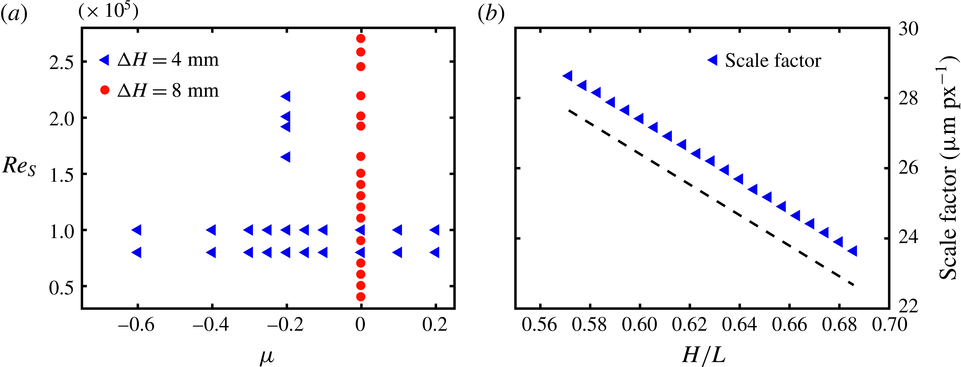
(a) Parameter space investigated within this paper in terms of the shear Reynolds number
 $Re_{S}$
and the rotation ratio
 $\unicode[STIX]{x1D707}$
. Blue triangles represent measurements over an axial height of
 $80~\text{mm}$
with a spacing of
 $4~\text{mm}$
; red circles with a spacing of
 $8~\text{mm}$
. (b) Scale factor at the 21 height positions. The dashed line serves as a guide for the eye.
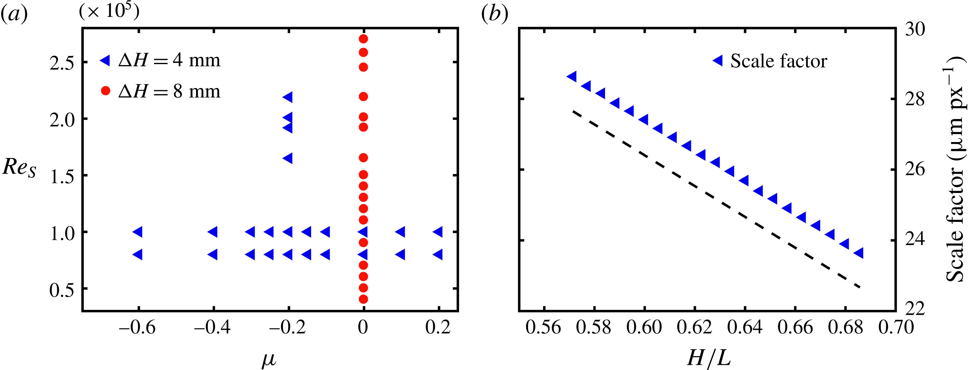
The parameter space investigated within this paper is shown in figure 2(a). At
 $Re_{S}=8\times 10^{4}$
and
 $Re_{S}=10^{5}$
, measurements are carried out for rotation ratios between
 $\unicode[STIX]{x1D707}=+0.2$
and
 $\unicode[STIX]{x1D707}=-0.6$
. Additionally, at the torque maximum (
 $\unicode[STIX]{x1D707}_{max}=-0.2$
) and for an outer cylinder at rest (
 $\unicode[STIX]{x1D707}=0$
), we analysed the flow in the range of
 $1.65\times 10^{5}\leqslant Re_{S}\leqslant 2.01\times 10^{5}$
and
 $4\times 10^{4}\leqslant Re_{S}\leqslant 2.7\times 10^{5}$
, respectively. The flow states are recorded at 21 axial positions with a relative displacement of
 $\unicode[STIX]{x0394}z=4~\text{mm}$
. Owing to the observed reduced axial dependence of the flow in the case of an outer cylinder at rest, which will be shown in § 3.1, the axial spacing was doubled to
 $\unicode[STIX]{x0394}z=8~\text{mm}$
for
 $\unicode[STIX]{x1D707}=0$
. To guarantee reproducibility of the measurements, a fixed protocol was used to adjust all investigated flow states. Starting at a resting flow and room temperature of
 $20\,^{\circ }\text{C}$
, the IC is driven up slowly to its final speed before the OC is accelerated. Then, a waiting time of approximately 10 min is used to ensure a stable flow state. During this waiting time, the interval
 $\unicode[STIX]{x0394}t$
between the laser pulses is adjusted to enclose the particle displacement between 4 and 8 pixels, leading to
 $70~\unicode[STIX]{x03BC}\text{s}\leqslant \unicode[STIX]{x0394}t\leqslant 870~\unicode[STIX]{x03BC}\text{s}$
for the investigated parameter space. The measurements start at the highest cylinder position and end up at the lowest one. After each measurement the traverse with the light sheet is shifted
 $4~\text{mm}$
or
 $8~\text{mm}$
downwards and the camera focus is adjusted to the new position. Each measurement consists of
 $150$
double images recorded at 15 Hz, leading to a measurement time of 10 s for each height. In the case of an OC at rest, this corresponds to 39–263 rotations of the IC, and for
 $Re_{S}=10^{5}$
and different
 $\unicode[STIX]{x1D707}$
between
 $50$
and
 $100$
IC rotations and between 9 and 36 OC rotations. During one run including 21 height steps the increase of the fluid temperature due to friction did not exceed
 $1\,^{\circ }\text{C}$
.
2.1 Measurement uncertainties
Within this study different uncertainties are concerned to quantify the accuracy of our measurements. As we use a subpixel interpolation scheme for the PIV algorithm to detect the correlation peak, the resolvable displacement for a single measurement is limited to
 $\unicode[STIX]{x1D6E5}_{SM}=0.1~\text{px}$
according to Nobach & Bodenschatz (Reference Nobach and Bodenschatz2009). The standard error of the mean follows as
 $\unicode[STIX]{x1D6E5}_{mean}=\unicode[STIX]{x1D6E5}_{SM}/\sqrt{N}$
with
 $N$
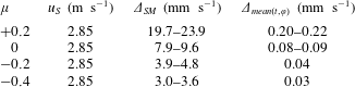
reflecting the number of individual measurements in terms of snapshots and spatial grid points used for the average. In table 2 the errors of the velocity measurements are exemplified for
 $Re_{S}=10^{5}$
.
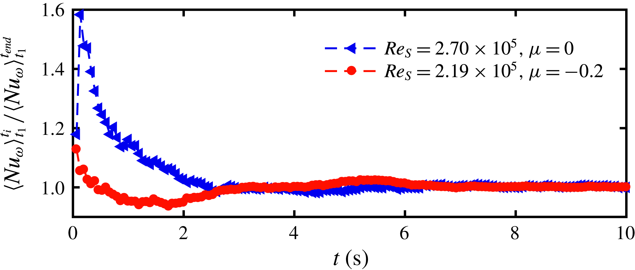
Temporal sliding average of the Nusselt number for the highest shear Reynolds number of
 $Re_{S}=2.70\times 10^{5}$
at
 $\unicode[STIX]{x1D707}=0$
and
 $Re_{S}=2.19\times 10^{5}$
at
 $\unicode[STIX]{x1D707}=-0.2$
, respectively. Convergence is reached at approximately a measurement time of 8 s.

Measurement uncertainty range for the 21 height positions due to a limited resolvable particle displacement detection for
 $Re_{S}=10^{5}$
and different
 $\unicode[STIX]{x1D707}$
.
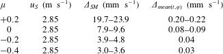
The error of a single measurement does not exceed 0.84 % of the shear velocity and the standard error of the mean over
 $t$
and
 $\unicode[STIX]{x1D711}$
not even 0.008 %. A second important source of uncertainty results from the small number of snapshots of 150 image pairs or rather the short measurement time of 10 s. It has been chosen that small because the temperature of the experiment is not actively controllable and the vortices have to be stable for the 21 height measurements performed during one run. However, we are investigating fully turbulent flows, which means that a large number of snapshots are needed to get statistically converged results. We can quantify this convergence based on the Nusselt number computed from the velocity fields according to § 4.2 for the highest shear Reynolds numbers investigated at
 $\unicode[STIX]{x1D707}=0$
and
 $\unicode[STIX]{x1D707}=-0.2$
by calculating a sliding average over time.
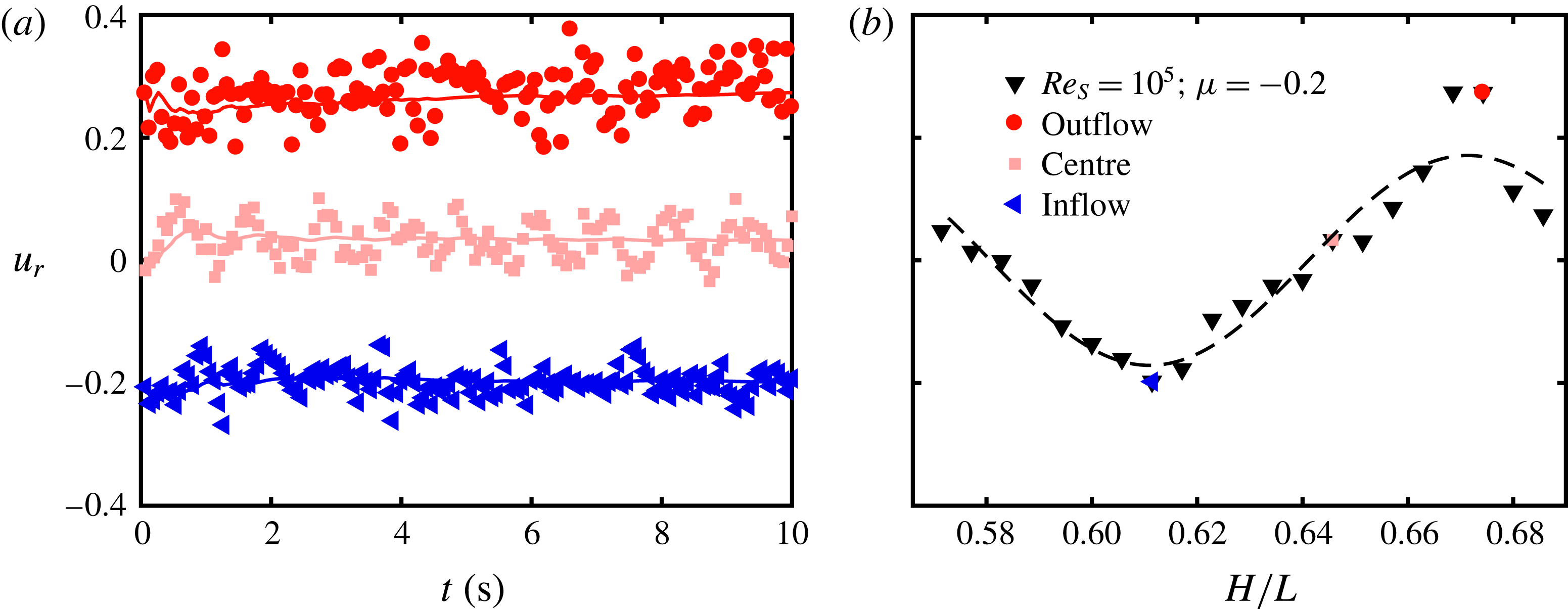
According to figure 3 the Nusselt number converges at approximately 8 s. The remaining statistical uncertainty is calculated by taking the standard deviation over the last 2 s related to its mean, reaching 0.24 % and 0.12 % for the exemplified cases. Further, in figure 4 the time signal of the azimuthally averaged radial velocity component in the inflow, vortex centre and outflow region at the middle of the gap together with the corresponding temporal averaged axial profile for
 $Re_{S}=10^{5}$
and
 $\unicode[STIX]{x1D707}=-0.2$
are depicted.
(a) Time signal of the azimuthally averaged radial velocity component
 $u_{r}$
in the centre of the gap at the axial height of the vortex inflow (blue triangles), centre (pink squares) and outflow (red circles). Lines represent the corresponding temporal sliding average. (b) Temporal and azimuthally averaged axial profile of the radial velocity component. Inflow, vortex centre and outflow are highlighted according to the time signal of (a). The dashed line is a fitted sinusoidal function as a guide for the eye.

Obviously, the vortices at the torque maximum are stable for the measurement time and result in an axial profile, which deviates from a sinusoidal shape especially in the inflow region, in contrast to laminar Taylor vortices. Therefore, the choice of 150 snapshots taken over 10 s is a suitable trade-off between statistical convergence, temperature increase and vortex stability.
Finally, we also calculate axial averaged flow properties within this paper, which requires an exact average length of one vortex pair. According to figure 4, our height scan consisting of 21 equally spaced axial positions covers nearly the length of a vortex pair up to approximately one height step missing. The corresponding error becomes largest at the rotation ratio of the torque maximum, where the axial dependence of the flow is most pronounced. Therefore, we quantify this error for
 $\unicode[STIX]{x1D707}=-0.2$
assuming that the adjacent vortices of the measurement volume have the same shape as the measured one. Thus, we can simply add an additional, hypothetical height position below the measurement volume with the same flow state as for the top axial position to close the vortex pair. Exemplified on the axial profile of figure 4(b), we add a
 $u_{r}$
value at
 $H/L=0.691$
identical to the one at
 $H/L=0.571$
. The calculated deviation from our original result yields an estimation for this uncertainty. Within the following sections all three measurement uncertainties are taken into account by the root mean square of the individual ones. Most error bars are within the size of the used symbols and therefore not shown.
3 Flow field analysis
3.1 Influence of the rotation ratio on the flow structure
The TC flow, where both cylinders rotate independently, can be distinguished into three regimes concerning the rotation ratio
 $\unicode[STIX]{x1D707}$
, namely co-rotation (
 $\unicode[STIX]{x1D707}>0$
), low counter-rotation (
 $\unicode[STIX]{x1D707}_{max}\leqslant \unicode[STIX]{x1D707}<0$
) and high counter-rotation (
 $\unicode[STIX]{x1D707}<\unicode[STIX]{x1D707}_{max}$
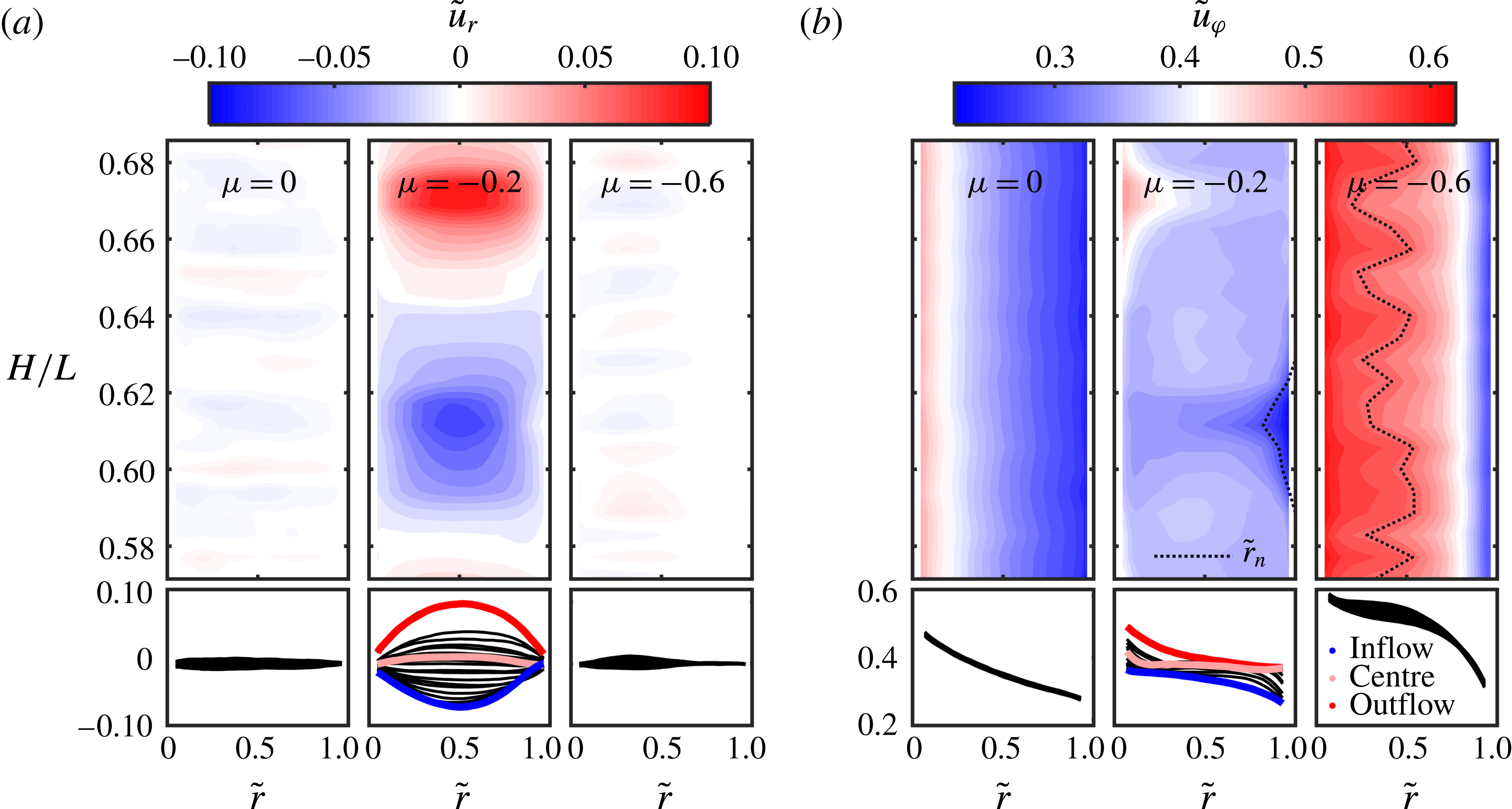
). The flow for an outer cylinder at rest is between the first two mentioned regimes. In figure 5 different flow regimes are illustrated for a shear Reynolds number of
 $Re_{S}=10^{5}$
and the rotation ratios
 $\unicode[STIX]{x1D707}=0$
,
 $\unicode[STIX]{x1D707}=-0.2$
and
 $\unicode[STIX]{x1D707}=-0.6$
. On the bottom part of each panel the temporal and azimuthally averaged (
 $t,\unicode[STIX]{x1D711}$
) radial and azimuthal velocity profiles for 21 height positions are depicted, and these are compounded in the contour plot above. The radial coordinate in normalized units is defined as
 $\tilde{r}=(r-r_{1})/(r_{1}-r_{2})$
, leading to
 $\tilde{r}(r=r_{1})=0$
at the inner cylinder and
 $\tilde{r}(r=r_{2})=1$
at the outer one. Also the azimuthal velocity component is mapped to an interval between 0 and 1 concerning the cylinder speeds:
 $\tilde{u} _{\unicode[STIX]{x1D711}}=(u_{\unicode[STIX]{x1D711}}-u_{\unicode[STIX]{x1D711},2})/(u_{\unicode[STIX]{x1D711},1}-u_{\unicode[STIX]{x1D711},2})$
with
 $u_{\unicode[STIX]{x1D711}}=\unicode[STIX]{x1D714}r$
. Based on the definition of the shear Reynolds number a shear velocity
 $u_{S}$
is defined to normalize the radial velocity component
 $\tilde{u} _{r}=u_{r}/u_{S}$
with
 $$\begin{eqnarray}u_{S}=\frac{2}{1+\unicode[STIX]{x1D702}}|\unicode[STIX]{x1D702}u_{\unicode[STIX]{x1D711},2}-u_{\unicode[STIX]{x1D711},1}|.\end{eqnarray}$$
This velocity provides a reference for general rotating shear flows from a dynamical point of view.
Contour plots and velocity profiles of the temporal and azimuthally averaged, normalized (a) radial
 $\tilde{u} _{r}$
and (b) azimuthal velocity component
 $\tilde{u} _{\unicode[STIX]{x1D711}}$
at 21 different heights for
 $Re_{S}=10^{5}$
and the rotation ratios
 $\unicode[STIX]{x1D707}=0,-0.2,-0.6$
. Profiles at the axial position of the inflow, outflow and centre of a turbulent Taylor vortex for
 $\unicode[STIX]{x1D707}=-0.2$
are highlighted in blue, red and pink, respectively. The dotted lines indicate the position of the neutral surface
 $\tilde{r}_{n}$
, which is analysed in § 3.3. The representation of the colour maps of the contour plots is based on a bilinear interpolation.

For pure inner cylinder rotation (
 $\unicode[STIX]{x1D707}=0$
), the time and azimuthally averaged radial velocity is close to zero all over the gap, with only weak strips of positive and negative velocity alternating in the axial direction. These strips can be interpreted as the remnants of turbulent Taylor vortices inside the flow. Therefore, the azimuthal velocity component only changes noticeably with the radial coordinate direction and the corresponding height profiles collapse onto one line. When the rotation ratio is decreased to
 $\unicode[STIX]{x1D707}=-0.2$
, strong vortices are present in the flow and fill the whole gap. In the in- and outflow regions, angular velocity is transported strongly from the cylinders in the wall-normal direction, causing an enhanced angular momentum transport. The evolution of these roll structures is assumed to generate a maximum in torque. Further, the velocity profiles vary clearly with the axial position. The radial velocity profiles are distributed quite symmetrically about the zero line, while the azimuthal profiles surround a nearly horizontal line with a non-zero amount. This flat azimuthal profile corresponds to the axial position of the vortex centre. When
 $\unicode[STIX]{x1D707}$
is decreased to
 $\unicode[STIX]{x1D707}=-0.6$
, the flow changes again significantly. The axial dependence of the profiles is now restricted to an inner part of the gap and the roll structures only exist in that inner region. In the outer gap region the flow is stabilized by the outer cylinder rotation leading back to a mainly radial dependence of the azimuthal velocity. These results are in good agreement with the findings of van der Veen et al. (Reference van der Veen, Huisman, Merbold, Harlander, Egbers, Lohse and Sun2016) at the same radius ratio and those of Ostilla-Mónico et al. (Reference Ostilla-Mónico, van der Poel, Verzicco, Grossmann and Lohse2014b
) at
 $\unicode[STIX]{x1D702}=0.714$
.
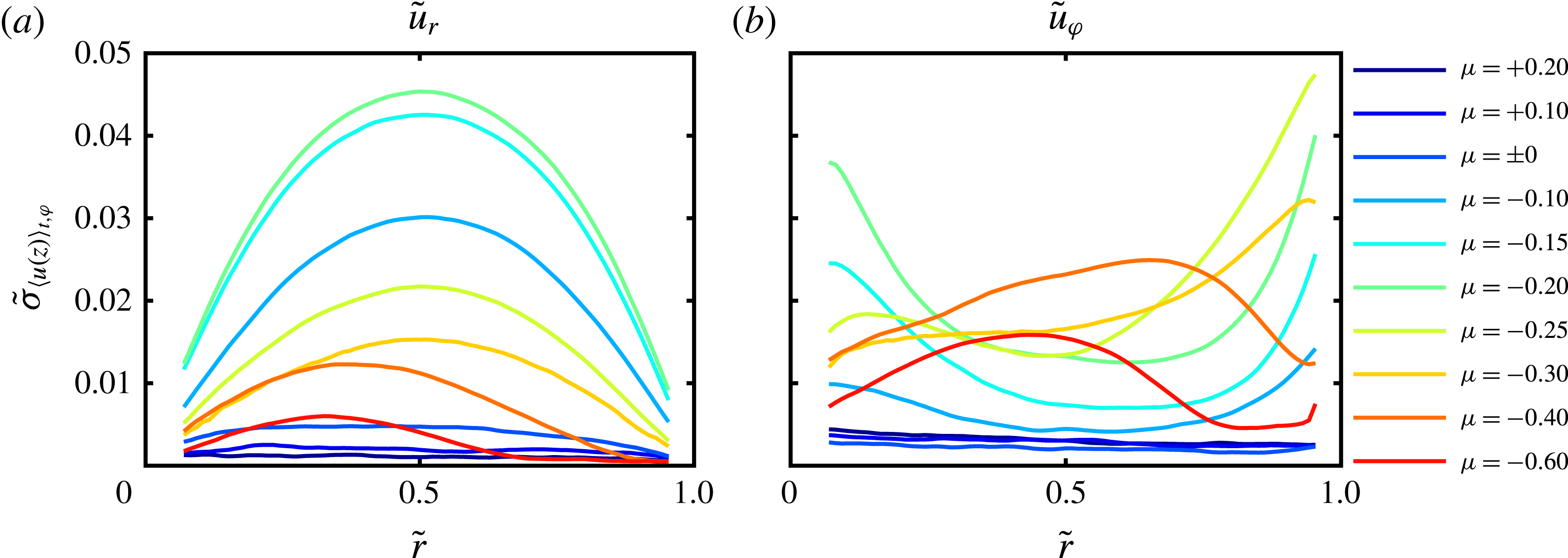
To analyse the evolution of the axial dependence with decreasing rotation ratio in more detail, we further calculate the standard deviation of the temporal and azimuthally averaged velocity components at each radial position across the 21 heights for
 $Re_{S}=10^{5}$
. The result is depicted in figure 6.
Standard deviation of the temporal and azimuthally averaged (a) radial and (b) azimuthal velocity components at each radial position across the 21 heights at the shear Reynolds number
 $Re_{S}=10^{5}$
and different rotation ratios
 $\unicode[STIX]{x1D707}$
.

For both co-rotating flow states the radial and azimuthal velocity profiles nearly do not deviate in the axial coordinate direction. For pure inner cylinder rotation, axial dependence starts to develop in the radial velocity component with a larger amount near the inner cylinder, while the azimuthal velocity profiles still do not change. In the low counter-rotating regime, turbulent Taylor vortices are formed with an increasing strength, which is reflected by an increase of axial dependence in both profiles. The
 $\tilde{\unicode[STIX]{x1D70E}}_{\langle u_{r}(z)\rangle _{t,\unicode[STIX]{x1D711}}}$
profiles are symmetrically arranged around the centre of the gap with a growing maximum at
 $\tilde{r}=0.5$
. This maximum decreases for
 $\unicode[STIX]{x1D707}$
beyond
 $\unicode[STIX]{x1D707}_{max}$
and symmetry breaks at
 $\unicode[STIX]{x1D707}=-0.4$
. Here, the axial dependence of the profiles is restricted to the inner part of the gap and shifted away from the outer cylinder wall with decreasing
 $\unicode[STIX]{x1D707}$
. Accordingly, the standard deviation of the azimuthal velocity profiles in the axial direction increases first all over the gap, but it becomes more pronounced in the cylinder wall regions. For stronger counter-flow we see again the effect of the outer cylinder stabilization with a local maximum closer to the outer cylinder wall than in the case of the radial velocity component. This evolution of the height dependence of the velocity profiles clearly shows that the turbulent Taylor vortices are formed and strengthened in a continuous process while their breakdown in the outer gap region seems to happen suddenly.
3.2 Axially averaged velocity profiles
Temporal and spatial averaged (
 $t,\unicode[STIX]{x1D711},z$
) radial profiles of (a) the normalized angular velocity
 $\tilde{\unicode[STIX]{x1D714}}=(\unicode[STIX]{x1D714}-\unicode[STIX]{x1D714}_{2})/(\unicode[STIX]{x1D714}_{1}-\unicode[STIX]{x1D714}_{2})$
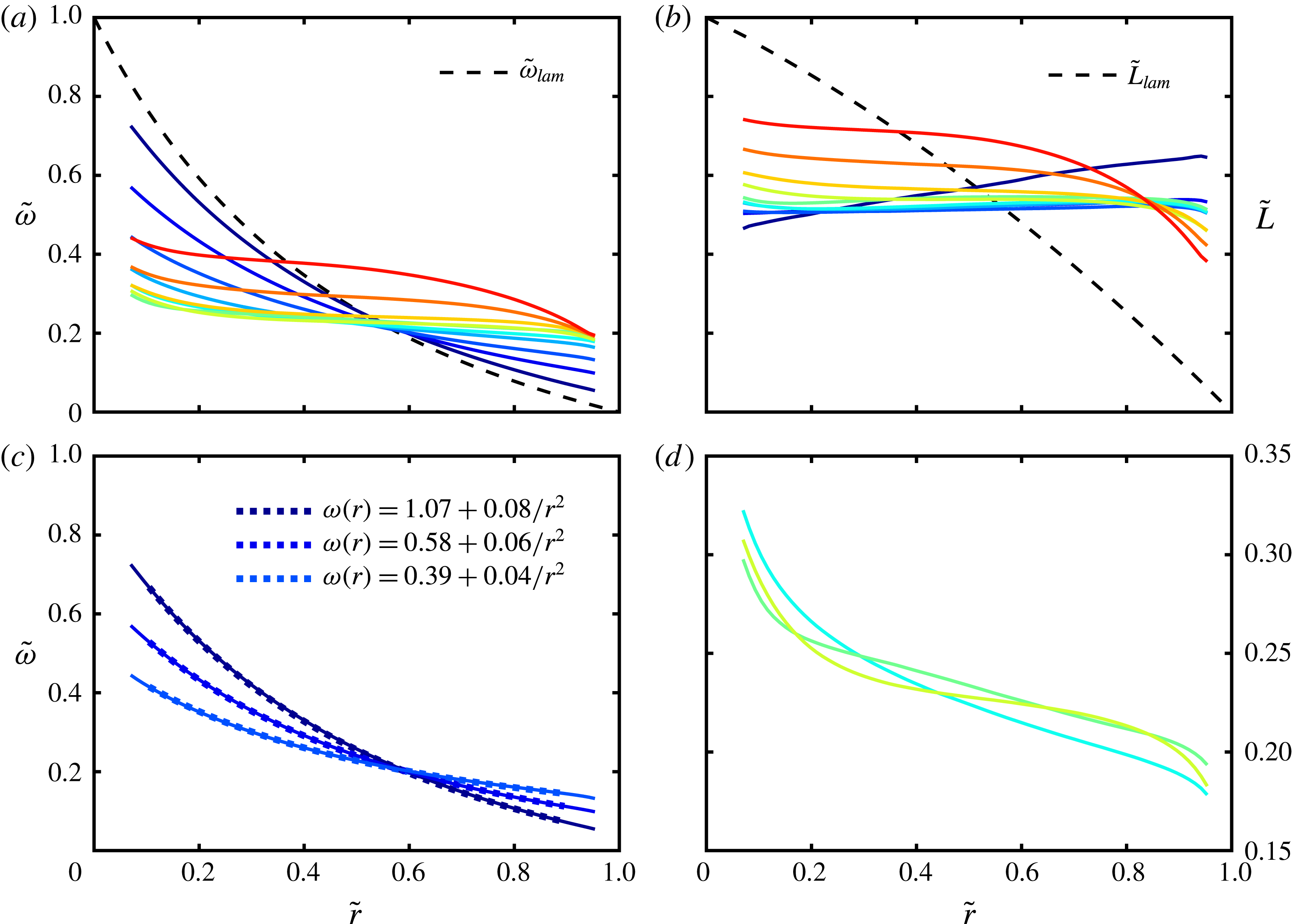
and (b) angular momentum
 $\tilde{L}=(L-L_{2})/(L_{1}-L_{2})$
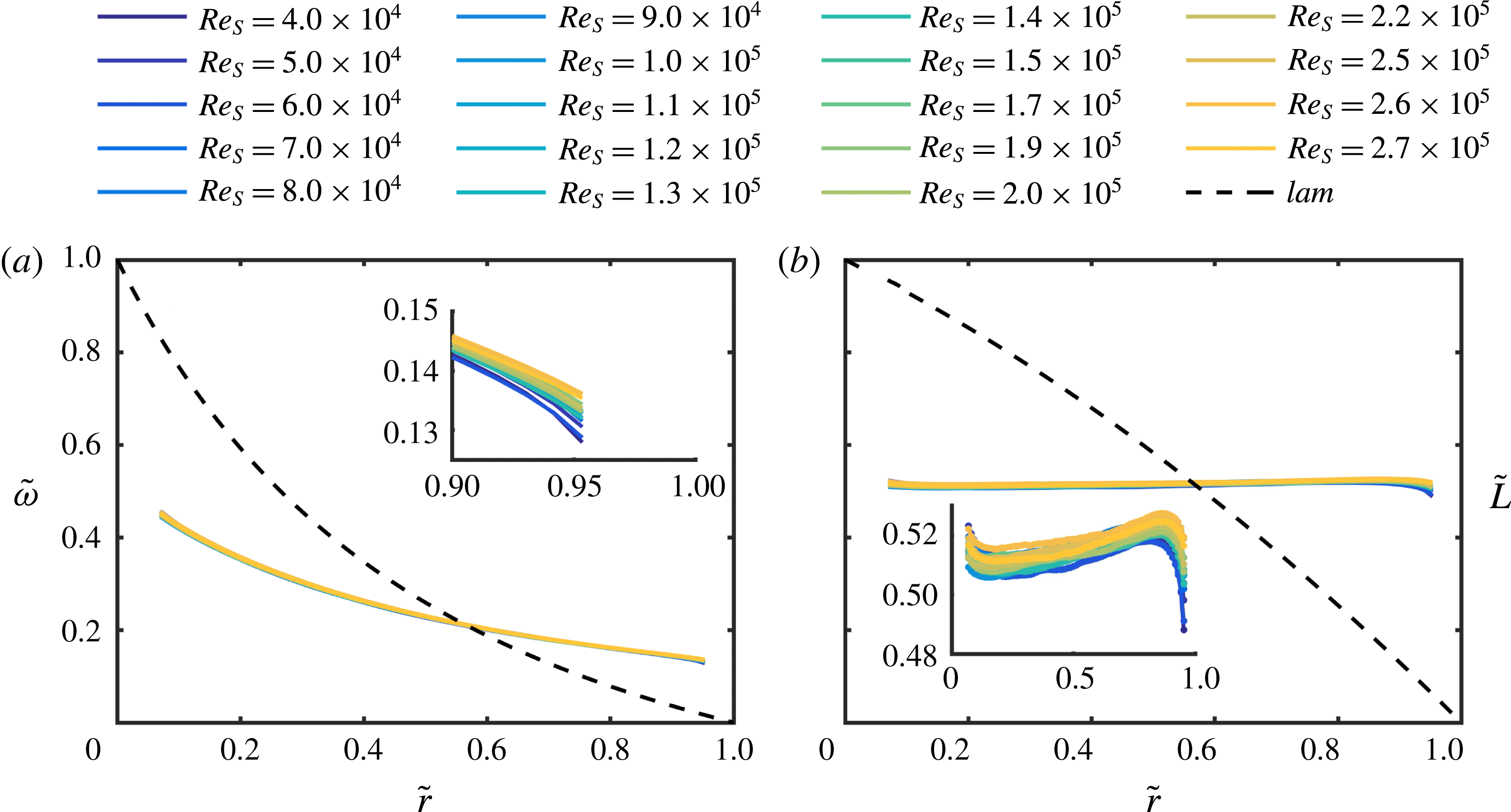
for pure inner cylinder rotation and different shear Reynolds numbers.

Temporal and spatial averaged (
 $t,\unicode[STIX]{x1D711},z$
) radial profiles of (a,c,d) the normalized angular velocity
 $\tilde{\unicode[STIX]{x1D714}}=(\unicode[STIX]{x1D714}-\unicode[STIX]{x1D714}_{2})/(\unicode[STIX]{x1D714}_{1}-\unicode[STIX]{x1D714}_{2})$
and (b) angular momentum
 $\tilde{L}=(L-L_{2})/(L_{1}-L_{2})$
for
 $Re_{S}=10^{5}$
and different
 $\unicode[STIX]{x1D707}$
. Colours are in accord with the legend of figure 6. In (c) the dotted lines represent bulk profiles based on the laminar Couette solution with boundaries
 $\unicode[STIX]{x1D714}_{1,i}(\tilde{r}=0.1)$
and
 $\unicode[STIX]{x1D714}_{2,i}(\tilde{r}=0.9)$
. In (d) the angular velocity profiles for
 $-0.15\leqslant \unicode[STIX]{x1D707}\leqslant -0.25$
are shown in more detail.

To better understand the influence of the rotation ratio
 $\unicode[STIX]{x1D707}$
and the shear Reynolds number
 $Re_{S}$
on the flow, we analyse the temporal and spatial averaged (
 $t,\unicode[STIX]{x1D711},z$
) radial profiles of the angular velocity
 $\tilde{\unicode[STIX]{x1D714}}=(\unicode[STIX]{x1D714}-\unicode[STIX]{x1D714}_{2})/(\unicode[STIX]{x1D714}_{1}-\unicode[STIX]{x1D714}_{2})$
and angular momentum
 $\tilde{L}=(L-L_{2})/(L_{1}-L_{2})$
with
 $L=r^{2}\unicode[STIX]{x1D714}$
. They can be compared to the laminar Couette solution, which is given by
 $$\begin{eqnarray}\unicode[STIX]{x1D714}_{lam}(r)=A+{\displaystyle \frac{B}{r^{2}}},\quad L_{lam}(r)=Ar^{2}+B,\end{eqnarray}$$
 $$\begin{eqnarray}A=-\unicode[STIX]{x1D714}_{1}{\displaystyle \frac{\unicode[STIX]{x1D702}^{2}-\unicode[STIX]{x1D707}}{1-\unicode[STIX]{x1D702}^{2}}},\quad B=\unicode[STIX]{x1D714}_{1}r_{1}^{2}{\displaystyle \frac{1-\unicode[STIX]{x1D707}}{1-\unicode[STIX]{x1D702}^{2}}}.\end{eqnarray}$$
When the laminar profile is normalized as the measured one, it becomes independent of the cylinder speeds and therefore of
 $\unicode[STIX]{x1D707}$
; thus
 $$\begin{eqnarray}\displaystyle & \displaystyle \tilde{\unicode[STIX]{x1D714}}_{lam}(r)={\displaystyle \frac{1}{1-\unicode[STIX]{x1D702}^{2}}}\left(\left({\displaystyle \frac{r_{1}}{r}}\right)^{2}-\unicode[STIX]{x1D702}^{2}\right), & \displaystyle\end{eqnarray}$$
 $$\begin{eqnarray}\displaystyle & \displaystyle \tilde{L}_{lam}(r)={\displaystyle \frac{1}{1-\unicode[STIX]{x1D702}^{2}}}\left(1-\left({\displaystyle \frac{r}{r_{2}}}\right)^{2}\right). & \displaystyle\end{eqnarray}$$
Figure 7 illustrates the influence of the shear Reynolds number in the case of
 $\unicode[STIX]{x1D707}=0$
. The normalized profiles collapse onto one line in the bulk flow, indicating a universal flow behaviour at infinite cylinder speed. Only near the cylinder walls is a deviation visible, reflecting the decrease of the boundary layer thickness with increasing Reynolds number. Specifically, the
 $L$
profiles are nearly flat with a slightly positive slope in the bulk and an amount of approximately
 $\tilde{L}\approx 0.5$
, the arithmetic mean of the angular momenta of the cylinder walls. The same result was found by Brauckmann et al. (Reference Brauckmann, Salewsky and Eckhardt2016) and linked to neutral stability of the profiles.
In figure 8(a) the averaged angular velocity profiles are depicted together with the laminar one at
 $Re_{S}=10^{5}$
for different rotation ratios. When
 $\unicode[STIX]{x1D707}$
is decreased from
 $+0.2$
to
 $-0.2$
, the profiles at first follow the laminar one quite well and then become continuously flatter until they are nearly horizontal at
 $\unicode[STIX]{x1D707}=\unicode[STIX]{x1D707}_{max}$
. For higher counter-rotation rates beyond the maximum regime, they are shifted in the inner bulk region to higher values and adapt in the outer bulk region more and more to the laminar profile. Therefore, the torque maximum seems to coincide with the smallest gradient of angular velocity in the bulk flow, reflecting an effective mixing. Similar investigations at a much lower shear Reynolds number of approximately
 $Re_{S}=3950$
have been done by Ostilla-Mónico et al. (Reference Ostilla-Mónico, Huisman, Janninik, van Gils, Verzicco, Grossmann and Lohse2014a
), who found the same change of profile shape. Their profiles show in addition the expected difference in boundary layer thickness at the inner and outer cylinder, as they reach far inside the gap at low Reynolds numbers.
In figure 8(b) the same profiles are shown in terms of the angular momentum. For co- and weak counter-rotating flow states, the profiles are flat in the bulk with an amount of
 $\tilde{L}\approx 0.5$
except for
 $\unicode[STIX]{x1D707}=+0.2$
. There, the profile exhibits a strong positive slope, which is a consequence of the normalization process as
 $L_{1}-L_{2}$
goes to zero when
 $\unicode[STIX]{x1D707}$
approaches the Rayleigh stability line of
 $\unicode[STIX]{x1D707}=\unicode[STIX]{x1D702}^{2}=0.25$
. For higher counter-rotation the
 $L$
profiles are shifted upwards in the inner bulk region, while the slope becomes more and more negative in the outer one. The sensitivity of the shape of the
 $L$
profiles to changes in
 $\unicode[STIX]{x1D707}$
in the high counter-rotating regime is more pronounced than for the
 $\unicode[STIX]{x1D714}$
profiles and the opposite is true for
 $\unicode[STIX]{x1D707}>\unicode[STIX]{x1D707}_{max}$
.
Before we analyse the average radial gradient of angular velocity and angular momentum in the bulk flow, we shall have a closer look at the profile shape of the angular velocity for the co- and low counter-rotating regime. For
 $\unicode[STIX]{x1D707}\geqslant 0$
we can separate the flow into three regions with free surfaces in between: inner and outer boundary layer (BL) and the bulk. Of course, the question arises where the BLs end and the bulk starts. In general in TC systems with small radius ratios a considerable difference between the inner (
 $\unicode[STIX]{x1D706}_{1}$
) and outer BL thickness (
 $\unicode[STIX]{x1D706}_{2}$
) is expected. An estimation of this difference proposed by Eckhardt, Grossmann & Lohse (Reference Eckhardt, Grossmann and Lohse2007a
) is based on the assumption that the mean angular velocity in the bulk is equal to the average velocity of the cylinders. This would lead to
 $\unicode[STIX]{x1D706}_{1}/\unicode[STIX]{x1D706}_{2}\approx \unicode[STIX]{x1D702}^{3}=1/8$
. However, this assumption does not fit the results of Ostilla-Mónico et al. (Reference Ostilla-Mónico, Huisman, Janninik, van Gils, Verzicco, Grossmann and Lohse2014a
), where the BL size difference was restricted to a factor of less than
 $1/3$
for our
 $\unicode[STIX]{x1D707}$
regime. Further, our measurements have been done at very high shear Reynolds numbers, where the size of the BLs is smaller than our closest measurement point to the wall. So, we can fix the proposed bulk system to the borders of
 $\tilde{r}_{1,i}=0.1$
and
 $\tilde{r}_{2,i}=0.9$
, keeping in mind that the possible asymmetry of BL thickness is not inside our field of view. These borders will also be used in the following sections whenever a radial average across the bulk flow is needed. With the wall velocities of the bulk system coinciding with the locally measured angular velocities at
 $\tilde{r}_{1,i}=0.1$
and
 $\tilde{r}_{2,i}=0.9$
, we calculate the hypothetical laminar Couette solution in the bulk system and find perfect agreement with the measured velocity profiles for
 $\unicode[STIX]{x1D707}\geqslant 0$
(see figure 8
c). Therefore, the angular velocity in the bulk flow is inversely proportional to the square of the radial coordinate (
 $1/r^{2}$
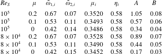
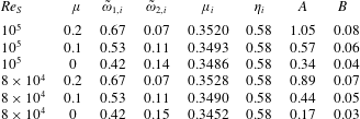
). In table 3 the main parameters of the fitted laminar Couette profile in the bulk system are summarized. When the shear Reynolds number is kept constant and the rotation ratio
 $\unicode[STIX]{x1D707}$
is decreased from
 $+0.2$
to
 $0$
, the parameters
 $A$
and
 $B$
according to (3.3) with the corresponding bulk system values are positive and decreasing. As
 $A$
is positive, the Rayleigh stability condition
 $\unicode[STIX]{x1D707}_{i}>\unicode[STIX]{x1D702}_{i}^{2}$
is fulfilled, but the flow state comes closer to the stability border
 $\unicode[STIX]{x1D707}_{i}=\unicode[STIX]{x1D702}_{i}^{2}$
with decreasing
 $\unicode[STIX]{x1D707}$
. Further, a decreasing value of
 $B$
represents a decreasing magnitude of the angular velocity gradient at a specific radial position
 $r$
. To the best of our knowledge this is the first evidence for a shape similarity between the laminar Couette solution and fully turbulent bulk profiles of angular velocity for pure inner cylinder rotation and co-rotation. This goes far beyond the finding of Brauckmann et al. (Reference Brauckmann, Salewsky and Eckhardt2016), who reported that
 $\unicode[STIX]{x1D714}_{lam}$
can be used as an approximation for the magnitude of the turbulent mean profile in the centre of the gap. We hope that our result will motivate other researchers to further analyse this similarity.
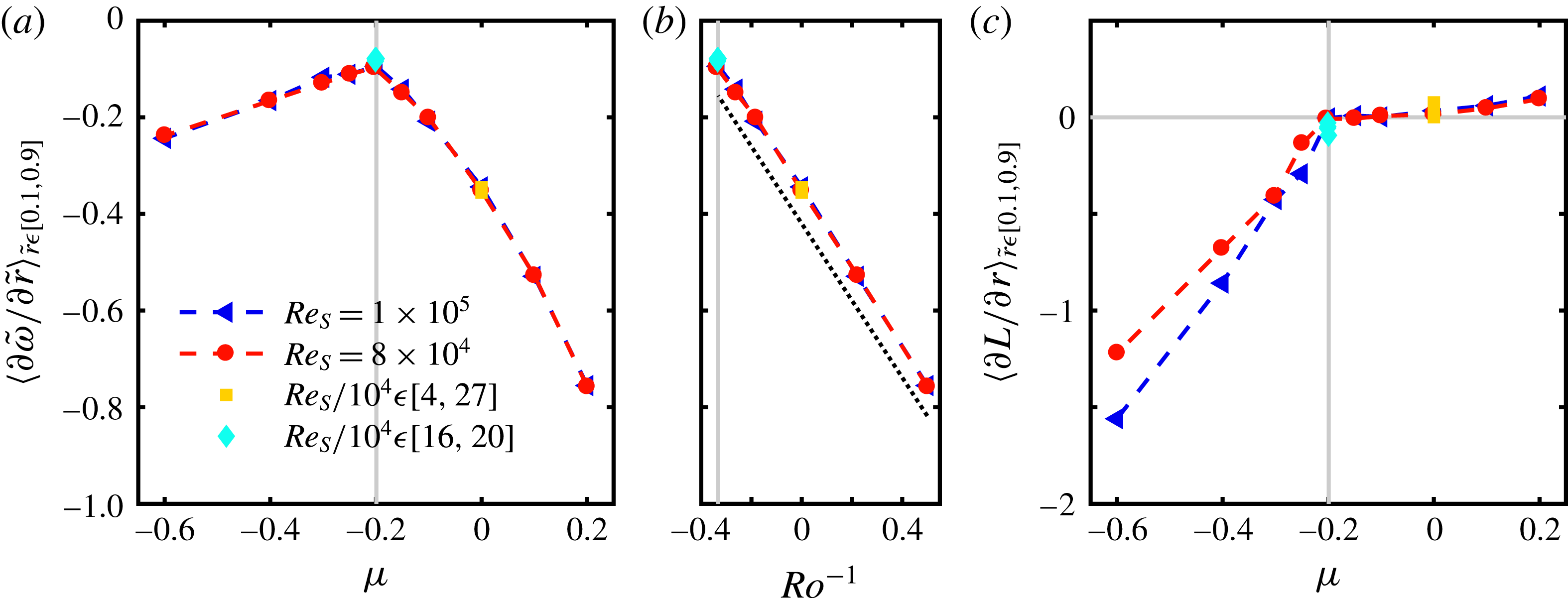
Normalized radial gradient of angular velocity profiles as a function of (a)
 $\unicode[STIX]{x1D707}$
and (b)
 $Ro^{-1}$
, and (c) radial gradient of angular momentum profiles as a function of
 $\unicode[STIX]{x1D707}$
averaged over
 $\tilde{r}\in [0.1,0.9]$
. Blue triangles and red circles represent results for
 $Re_{S}=10^{5}$
and
 $Re_{S}=8\times 10^{4}$
for different rotation ratios, respectively. Yellow squares and cyan diamonds indicate measurements at
 $\unicode[STIX]{x1D707}=0$
and
 $\unicode[STIX]{x1D707}=-0.2$
for different
 $Re_{S}$
, respectively. Grey vertical lines mark the location of the torque maximum. The dotted line in (b) serves as a guide for the eye.

Parameters of the hypothetical laminar Couette profile in the bulk TC system:
 $\tilde{\unicode[STIX]{x1D714}}_{1,i}$
and
 $\tilde{\unicode[STIX]{x1D714}}_{2,i}$
represent the values of angular velocity at
 $\tilde{r}=0.1$
and
 $\tilde{r}=0.9$
, respectively;
 $\unicode[STIX]{x1D707}_{i}$
,
 $\unicode[STIX]{x1D702}_{i}$
,
 $A$
and
 $B$
are the corresponding rotation ratio, radius ratio and coefficients of (3.3) of the bulk system.
In figure 8(d) also the three
 $\unicode[STIX]{x1D714}$
profiles close to the torque maximum are shown to further quantify the gradient differences. In the case of
 $\unicode[STIX]{x1D707}=-0.15$
the profile shows a nearly linear shape in the centre and outer bulk section. At the rotation ratio of the torque maximum, this linear section is enlarged into the region of the inner cylinder and the amount of the slope decreases. The profile shape changes again clearly at
 $\unicode[STIX]{x1D707}=-0.25$
, where in the centre of the gap the local gradient is further decreased, while in the inner and outer bulk region, the gradient increases strongly. In conclusion, the locally smallest amount of angular velocity gradient is reached beyond the torque maximum rotation ratio, while at
 $\unicode[STIX]{x1D707}=\unicode[STIX]{x1D707}_{max}$
the profile has a long region of small constant gradient. To compare now the
 $\unicode[STIX]{x1D714}$
gradients in the bulk flow for different
 $\unicode[STIX]{x1D707}$
we have to average the local values over the whole length of the bulk due to its strong dependence on the radial location. For consistency, the same procedure is used for the angular momentum. In figure 9 the normalized radial gradient of angular velocity and the radial gradient of angular momentum averaged over
 $\tilde{r}\in [0.1,0.9]$
are depicted. As we do not use the normalized form of
 $L$
, we prevent the strong positive slope at
 $\unicode[STIX]{x1D707}=+0.2$
resulting out of the normalization procedure.
The normalized radial gradient of angular velocity is negative for all shear Reynolds numbers and rotation ratios because the normalized profiles are mapped to an interval of 1 at the inner and 0 at the outer cylinder. We find the smallest amount of gradient at the rotation ratio of the torque maximum, and the increase of the angular velocity gradient magnitude is stronger for
 $\unicode[STIX]{x1D707}>\unicode[STIX]{x1D707}_{max}$
than for
 $\unicode[STIX]{x1D707}<\unicode[STIX]{x1D707}_{max}$
. All investigated flow states match to one curve, illustrating that the normalized bulk profiles depend less on the shear Reynolds number for
 $Re_{S}\geqslant 4\times 10^{4}$
. Ostilla-Mónico et al. (Reference Ostilla-Mónico, Huisman, Janninik, van Gils, Verzicco, Grossmann and Lohse2014a
) also found the smallest gradient of angular velocity coinciding with the rotation ratio of
 $\unicode[STIX]{x1D707}_{max}$
at
 $\unicode[STIX]{x1D702}=0.5$
and
 $Re_{S}\leqslant 3950$
, while Brauckmann et al. (Reference Brauckmann, Salewsky and Eckhardt2016) could confirm this coincidence only for much smaller gaps (
 $\unicode[STIX]{x1D702}\geqslant 0.8$
) at
 $Re_{S}=2\times 10^{4}$
. The discrepancy is probably due to the difference in
 $Re_{S}$
, which could also explain the
 $Re_{S}$
dependence of the gradient in the higher counter-rotating regime reported by Ostilla-Mónico et al. (Reference Ostilla-Mónico, Huisman, Janninik, van Gils, Verzicco, Grossmann and Lohse2014a
). Further, the calculation of the gradient in the mentioned studies differs from ours due to limitations in our spatial resolution. However, for co- and low counter-rotation, Ostilla-Mónico et al. (Reference Ostilla-Mónico, Huisman, Janninik, van Gils, Verzicco, Grossmann and Lohse2014a
) as well as Brauckmann et al. (Reference Brauckmann, Salewsky and Eckhardt2016) found a linear relationship between the
 $\unicode[STIX]{x1D714}$
gradient and the inverse Rossby number
 $Ro^{-1}$
or rather the rotation number
 $R_{\unicode[STIX]{x1D6FA}}$
. For comparison, we also plotted the gradient of angular velocity against
 $Ro^{-1}=2\unicode[STIX]{x1D707}d/(|1-\unicode[STIX]{x1D707}|r_{1})$
in figure 9(b) for co- and weak counter-rotation, identifying this linear relationship. In the case of the angular momentum, the gradient is slightly positive for
 $\unicode[STIX]{x1D707}>0$
and nearly zero at
 $\unicode[STIX]{x1D707}_{max}$
independent of
 $Re_{S}$
. In the higher counter-rotating regime the gradient decreases with decreasing
 $\unicode[STIX]{x1D707}$
and here the shear Reynolds number influences the slope of this decrease. However, the Reynolds-number dependence vanishes when also
 $L$
is normalized. Again, the bend, which coincides with
 $\unicode[STIX]{x1D707}_{max}$
in our study, is shifted to smaller
 $\unicode[STIX]{x1D707}$
in the study of Brauckmann et al. (Reference Brauckmann, Salewsky and Eckhardt2016), while the overall shape is the same.
3.3 Radial location of the neutral surface
The velocity profiles also give access to the neutral surface
 $r_{n}$
. It is the radial location in the gap, where the azimuthal velocity component
 $u_{\unicode[STIX]{x1D711}}$
vanishes. In the case of an inviscid fluid, this surface separates the linear stable from the linear unstable part of the flow and is defined according to Chandrasekhar (Reference Chandrasekhar1961) as
 $$\begin{eqnarray}r_{n,inv}(\unicode[STIX]{x1D707})=r_{1}\sqrt{\frac{1-\unicode[STIX]{x1D707}}{\unicode[STIX]{x1D702}^{2}-\unicode[STIX]{x1D707}}}.\end{eqnarray}$$
Once the cylinders are rotating in counter-direction, the neutral surface detaches from the outer cylinder wall. If the fluid is viscous, the secondary flow induced by the Taylor vortices can extend this theoretical line. Esser & Grossmann (Reference Esser and Grossmann1996) derived a prediction for the vortex extension called
 $r_{n,EG}$
, already expressed for TC flows by Brauckmann & Eckhardt (Reference Brauckmann and Eckhardt2013b
):
 $$\begin{eqnarray}r_{n,EG}(\unicode[STIX]{x1D707})=r_{1}+a(\unicode[STIX]{x1D702})(r_{n,inv}-r_{1}),\quad a(\unicode[STIX]{x1D702})=(1-\unicode[STIX]{x1D702})\left[\sqrt{\frac{(1+\unicode[STIX]{x1D702})^{3}}{2(1+3\unicode[STIX]{x1D702})}}-\unicode[STIX]{x1D702}\right]^{-1}.\end{eqnarray}$$
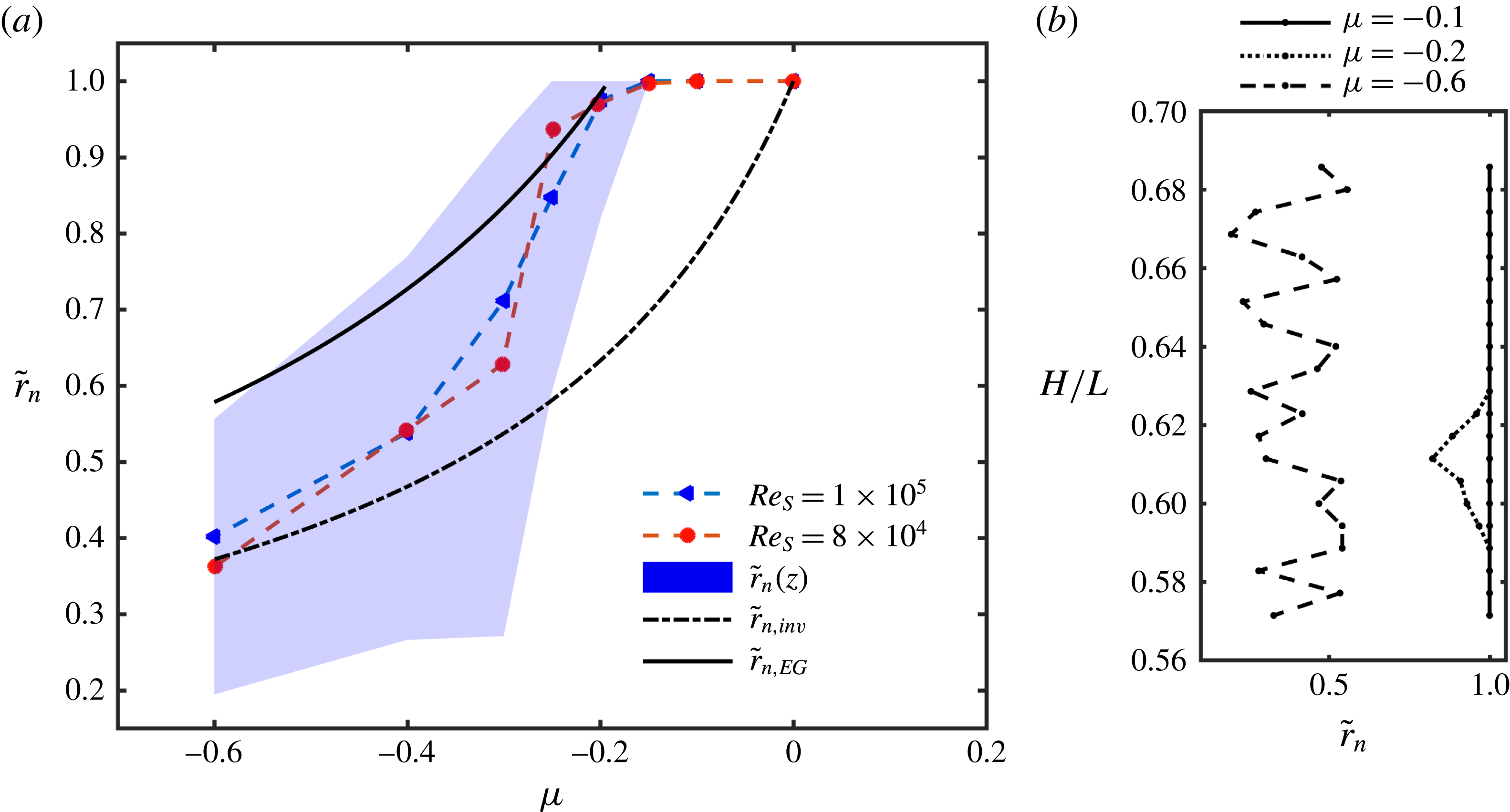
(a) Radial position of the normalized neutral surface
 $\tilde{r}_{n}$
for
 $Re_{S}=10^{5}$
(blue triangles) and
 $Re_{S}=8\times 10^{4}$
(red circles) as a function of the rotation ratio
 $\unicode[STIX]{x1D707}$
. The markers (triangles, circles) indicate the averaged position over time and space (
 $t,\unicode[STIX]{x1D711},z$
). The shaded area represents the deviation of the neutral surface along the axial coordinate direction. (b) Radial position of the neutral surface at different heights for
 $Re_{S}=10^{5}$
and
 $\unicode[STIX]{x1D707}=-0.1,-0.2,-0.6$
.

The prefactor in our configuration is
 $a(\unicode[STIX]{x1D702}=0.5)=1.5548$
. When the extension of the secondary flow reaches the outer cylinder wall, intermittency evolves, causing a radial inhomogeneity inside the gap. Brauckmann & Eckhardt (Reference Brauckmann and Eckhardt2013b
) showed that this onset of intermittency also works as a prediction for the torque maximum. By converting (3.7) with
 $r_{n,EG}(\unicode[STIX]{x1D707}_{max,EG})=r_{2}$
, the rotation ratio for the torque maximum is predicted at
 $\unicode[STIX]{x1D707}_{max,EG}=-0.191$
. In figure 10(a) the position of the neutral surface for our measurements is shown together with the two introduced predictions. The markers indicate the averaged values (
 $\langle \tilde{r}_{n}\rangle _{t,\unicode[STIX]{x1D711},z}$
) and the shaded area shows the range of this value for different axial positions. For both
 $Re_{S}$
the neutral surfaces are located on the outer cylinder wall or rather nested into the outer boundary layer, impossible to resolve until the rotation ratio is decreased to
 $\unicode[STIX]{x1D707}_{max}=-0.2$
, in good agreement with the prediction of EG and LDA measurements made by van Gils et al. (Reference van Gils, Grossmann, Sun and Lohse2012). Afterwards, its detachment starts first at the inflow region induced by the large-scale vortices inside the flow, leading to an axial dependence of
 $\tilde{r}_{n}$
(see figure 10
b). In the higher counter-rotating regime the averaged measurement results and the EG prediction move apart with decreasing
 $\unicode[STIX]{x1D707}$
and at
 $\unicode[STIX]{x1D707}=-0.6$
they seem to converge with the inviscid prediction. van Gils et al. (Reference van Gils, Grossmann, Sun and Lohse2012) also measured the position of the neutral surface closer to the inner cylinder than the inviscid prediction suggests for very strong counter-rotation; however, their measurements were only done at one cylinder height. The neutral surface
 $\tilde{r}_{n}$
becomes dependent on the
 $z$
-coordinate for
 $\unicode[STIX]{x1D707}\leqslant \unicode[STIX]{x1D707}_{max}$
and depicts its largest range at
 $\unicode[STIX]{x1D707}=-0.3$
, indicating the complete detachment of the neutral surface at all axial positions. Afterwards, the axial range decreases again with
 $\unicode[STIX]{x1D707}$
, which can be explained by the vortex size. When the neutral surface is shifted from the outer cylinder into the direction of the inner one, the effective gap width of the vortices decreases, which was already shown by Ostilla et al. (Reference Ostilla, Stevens, Grossmann, Verzicco and Lohse2013) for
 $\unicode[STIX]{x1D702}=0.714$
. Accordingly, smaller vortices lead to a smaller axial range in the location of the neutral surface. In summary, (3.7) predicts the start of the neutral surface detachment very well; however, it fails for higher counter-rotating rates. In that regime the inviscid prediction fits very well to our data, as the outer cylinder stabilization laminarizes large areas of the gap.
3.4 Energy distribution
The kinetic energy of the flow can offer a good insight into changes of the flow state concerning turbulent Taylor rolls, when the velocity field is decomposed into its large-scale and its turbulent contributions according to (Brauckmann & Eckhardt Reference Brauckmann and Eckhardt2013b )
 $$\begin{eqnarray}\boldsymbol{u}=\langle \boldsymbol{u}\rangle _{\unicode[STIX]{x1D711},t}+\boldsymbol{u}^{\prime \prime }=\bar{\boldsymbol{u}}+\boldsymbol{u}^{\prime \prime }.\end{eqnarray}$$
Then, the kinetic energy averaged over time and space (
 $t,\unicode[STIX]{x1D711},z$
) reads
 $$\begin{eqnarray}E_{kin}(r)={\textstyle \frac{1}{2}}\langle \bar{u}_{\unicode[STIX]{x1D711}}^{2}+\bar{u}_{r}^{2}+\bar{u}_{z}^{2}+{u_{\unicode[STIX]{x1D711}}^{\prime \prime }}^{2}+{u_{r}^{\prime \prime }}^{2}+{u_{z}^{\prime \prime }}^{2}\rangle _{t,\unicode[STIX]{x1D711},z}.\end{eqnarray}$$
The mixed terms vanish and the first term in (3.9) reflects the azimuthal base flow energy, which is the dominant quantity. To reveal the underlying flow structure, we neglect this energy portion. Further, we could not measure the axial velocity component within the horizontal planes, so we also have to set
 $u_{z}$
to zero. The remaining terms can be separated into the large-scale circulation energy
 $E_{LSC}$
and the turbulent kinetic energy
 $E_{TKE}$
:
 $$\begin{eqnarray}E_{LSC}(r)={\textstyle \frac{1}{2}}\langle \bar{u}_{r}^{2}\rangle _{t,\unicode[STIX]{x1D711},z},\quad E_{TKE}(r)={\textstyle \frac{1}{2}}\langle {u_{r}^{\prime \prime }}^{2}+{u_{\unicode[STIX]{x1D711}}^{\prime \prime }}^{2}\rangle _{t,\unicode[STIX]{x1D711},z}.\end{eqnarray}$$
These energies are summed to the total kinetic energy
 $E_{tot}(r)=E_{TKE}(r)+E_{LSC}(r)$
and normalized using the shear velocity:
 $\tilde{E}=E/E_{S}$
with
 $E_{S}=u_{S}^{2}/2$
. In figure 11 the different energy fractions are plotted as functions of
 $\tilde{r}$
and
 $\unicode[STIX]{x1D707}$
for
 $Re_{S}=8\times 10^{4}$
.
Contour plots of the temporal and spatial averaged (
 $t,\unicode[STIX]{x1D711},z$
), normalized kinetic energy fractions at
 $Re_{S}=8\times 10^{4}$
as functions of the normalized radius
 $\tilde{r}$
and the rotation ratio
 $\unicode[STIX]{x1D707}$
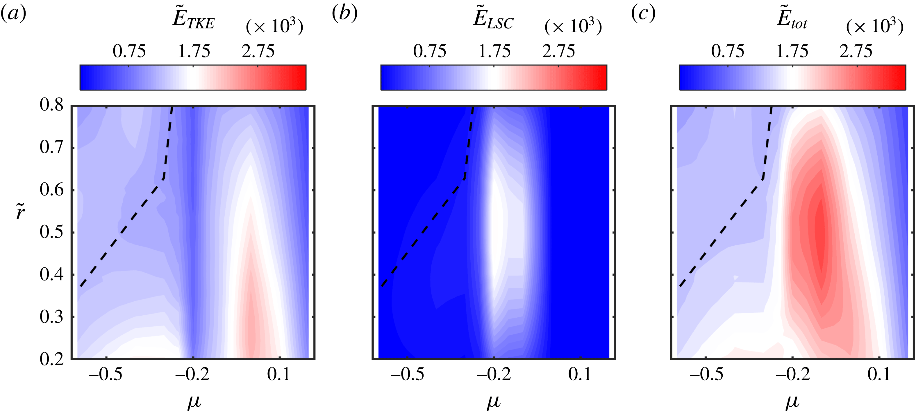
. The dashed line represents the location of the neutral surface (see figure 10). The representation of the colour maps of the contour plots is based on a bilinear interpolation.

The turbulent kinetic energy is larger for the inner than the outer gap region and becomes dominant for pure inner cylinder rotation. In the case of co-rotation the isolines have a curved shape, indicating a flow state close to the laminar one. At the rotation ratio of the torque maximum, the turbulent kinetic energy is reduced strongly, which illustrates a more coherent flow state induced by the formation of large-scale vortices. In the high counter-rotating regime the neutral line is located in an area of less turbulent kinetic energy, while in the inner and outer gap region, turbulence again increases slightly. Especially near the inner cylinder a small region of stronger fluctuations is present caused by the beginning of intermittency described by Brauckmann & Eckhardt (Reference Brauckmann and Eckhardt2013b
). The large-scale circulation energy is close to zero at co- and high counter-rotating flow states and depicts a pronounced maximum in the low counter-rotating regime at
 $\unicode[STIX]{x1D707}=\unicode[STIX]{x1D707}_{max}$
. While the increase of
 $\tilde{E}_{LSC}$
starting at
 $\unicode[STIX]{x1D707}=0$
seems to be smooth, its decrease happens rapidly for
 $\unicode[STIX]{x1D707}<\unicode[STIX]{x1D707}_{max}$
. The sum of both energy fractions results in a maximum of the total kinetic energy in the low counter-rotating regime at
 $\unicode[STIX]{x1D707}=-0.1$
shifted from the maximum of the large-scale circulation energy.
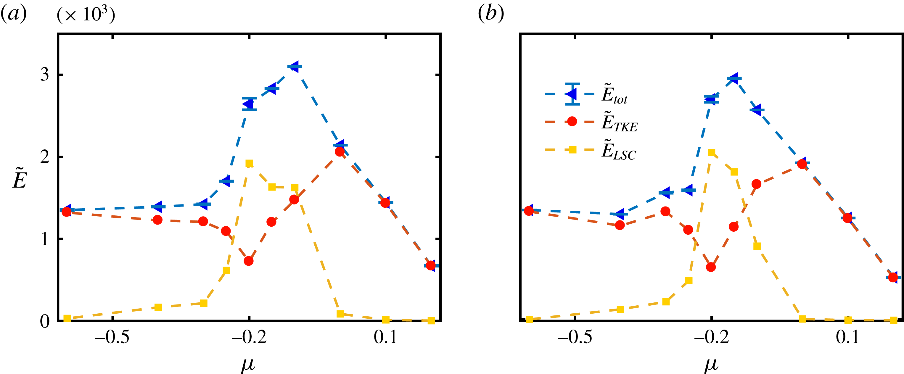
Temporal and spatial (
 $t,\unicode[STIX]{x1D711},z$
) averaged profiles of the normalized total energy
 $\tilde{E}_{tot}$
, turbulent energy
 $\tilde{E}_{TKE}$
and large-scale circulation energy
 $\tilde{E}_{LSC}$
in the centre of the gap (
 $\tilde{r}=0.5$
) for (a)
 $Re_{S}=8\times 10^{4}$
and (b)
 $Re_{S}=10^{5}$
.

In these energy calculations we could only consider two of the three velocity components. Therefore, in figure 12 we plot the energy fractions at the centre of the gap
 $(\tilde{r}=0.5)$
for
 $Re_{S}=8\times 10^{4}$
and
 $Re_{S}=10^{5}$
. Assuming that the axial velocity component of an idealized turbulent Taylor vortex vanishes in the centre of the gap, the error of the large-scale circulation energy calculated from a two-dimensional velocity field is reduced. Again, the large-scale circulation energy becomes maximal at the rotation ratio of the torque maximum, while the turbulent fraction exhibits a local minimum. For co- and strong counter-rotation
 $\tilde{E}_{LSC}$
vanishes and
 $\tilde{E}_{TKE}$
seems to converge in the high counter-rotating regime to a constant non-zero value. When we compare both measured Reynolds numbers, we see a pronounced difference in
 $\tilde{E}_{LSC}$
and
 $\tilde{E}_{tot}$
for
 $\unicode[STIX]{x1D707}=-0.1$
. This difference results from a change in the vortex state for
 $Re_{S}=8\times 10^{4}$
as shown in figure 13.
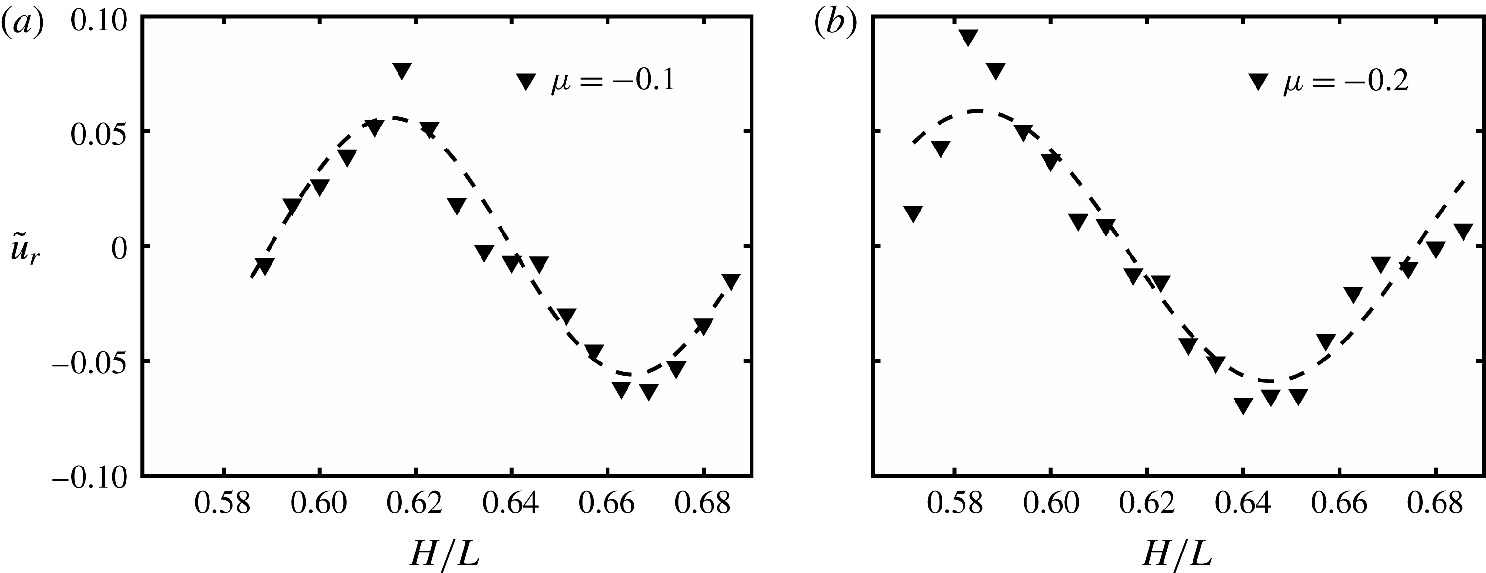
Axial profile of the averaged (
 $t,\unicode[STIX]{x1D711}$
) and normalized radial velocity component at
 $\tilde{r}=0.5$
for
 $Re_{S}=8\times 10^{4}$
and (a)
 $\unicode[STIX]{x1D707}=-0.1$
and (b)
 $\unicode[STIX]{x1D707}=-0.2$
. The dashed lines are fitted sinusoidal functions as a guide for the eye.

Despite our limited axial resolution of
 $4~\text{mm}$
, we can clearly see the different wavelengths of approximately
 $\unicode[STIX]{x1D706}(\unicode[STIX]{x1D707}=-0.1)\approx 0.97d$
and
 $\unicode[STIX]{x1D706}(\unicode[STIX]{x1D707}=-0.2)\approx 1.14d$
based on one vortex pair. According to Ostilla-Mónico et al. (Reference Ostilla-Mónico, van der Poel, Verzicco, Grossmann and Lohse2014b
) and Martinez-Arias et al. (Reference Martinez-Arias, Peixinho, Crumeyrolle and Mutabazi2014), a smaller wavelength of turbulent Taylor vortices and therefore a higher total number of vortices across the gap result in a larger transport of angular momentum in the classical regime and vice versa in the ultimate regime for
 $\unicode[STIX]{x1D702}=0.909$
. In contrast, Huisman et al. (Reference Huisman, van der Veen, Sun and Lohse2014) reported a higher Nusselt number for a smaller number of vortices in the ultimate regime for
 $\unicode[STIX]{x1D702}=0.716$
, measuring the torque only at a central segment of the inner cylinder. In our case for
 $\unicode[STIX]{x1D702}=0.5$
we are investigating flow states close to the transitional point between the classical and ultimate regimes (see § 4) and observe a higher total kinetic energy
 $\tilde{E}_{tot}$
and large-scale circulation energy
 $\tilde{E}_{LSC}$
at a smaller value of
 $\unicode[STIX]{x1D706}$
, comparing the data for
 $Re_{S}=8\times 10^{4}$
and
 $Re_{S}=10^{5}$
. Apparently, our findings support the results shown by Huisman et al. (Reference Huisman, van der Veen, Sun and Lohse2014). It is also worth mentioning that the change in wavelength illustrated in figure 13 is not a random event, as it was observed also by repeating the measurements. Up to this exceptional case, all flow states measured in the low counter-rotating regime within this study exhibit vortices of wavelengths of approximately 1.14 gap widths. Therefore, we can conclude that the rotation ratio of the torque maximum coincides with the maximum of
 $\tilde{E}_{LSC}$
and a local minimum of
 $\tilde{E}_{TKE}$
, while
 $\tilde{E}_{tot}$
maximizes at a slightly larger
 $\unicode[STIX]{x1D707}$
. Further, the large-scale circulation energy decreases strongly for
 $\unicode[STIX]{x1D707}<\unicode[STIX]{x1D707}_{max}$
, supporting the picture of a rapid breakdown of the vortices, as already shown in figure 6.
4 Scaling of the global response parameters
 $Re_{W}$
and
$Nu_{\unicode[STIX]{x1D714}}$


4.1 Wind Reynolds number
The wind Reynolds number
 $Re_{W}$
is a measure of the strength of the secondary flow (the so-called wind with components
 $u_{r}$
and
 $u_{z}$
) and is analysed based on the accessible radial velocity component
 $u_{r}$
. To estimate the amplitude of the wind, the standard deviation is used. As, in the low counter-rotating regime, turbulent Taylor vortices are present inside the gap, the wind amplitude is dominated by the variation of the velocity components in the axial direction. Therefore, we calculate
 $\unicode[STIX]{x1D70E}_{u_{r}}$
not only across time and the azimuthal coordinate direction, but also across the axial one:
 $\unicode[STIX]{x1D70E}_{u_{r}}=\unicode[STIX]{x1D70E}_{u_{r}(t,\unicode[STIX]{x1D711},z)}$
. The normalization is done again by use of the shear velocity. In figure 14 the radial profiles of the standard deviation of the radial velocity component
 $\tilde{\unicode[STIX]{x1D70E}}_{u_{r}}=\unicode[STIX]{x1D70E}_{u_{r}}/u_{S}$
are pictured.
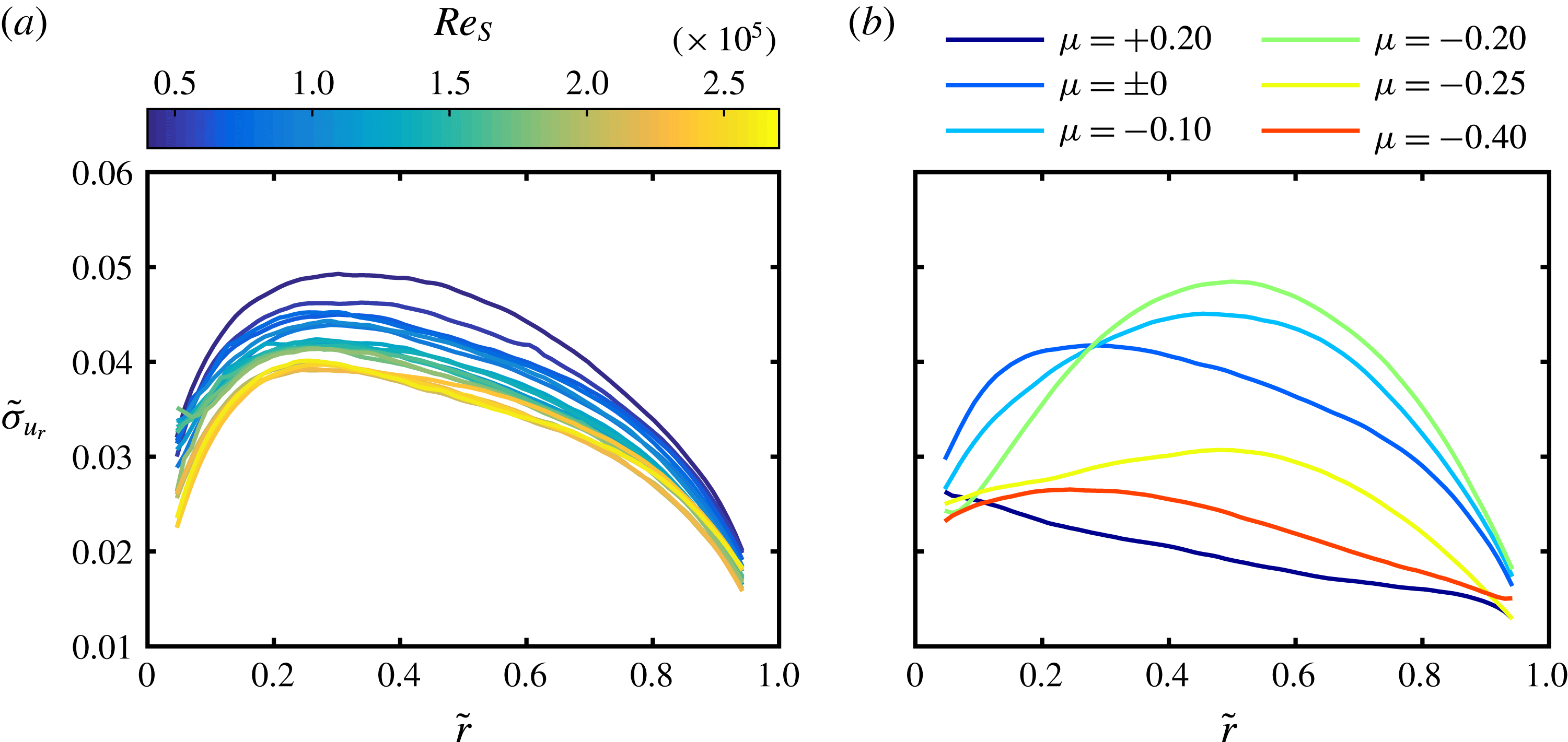
(a) Normalized radial profiles of the standard deviation of the radial velocity component
 $\tilde{\unicode[STIX]{x1D70E}}_{u_{r}}=\unicode[STIX]{x1D70E}_{u_{r}}/u_{S}$
calculated across time and space (
 $t,\unicode[STIX]{x1D711},z$
) for different
 $Re_{S}$
and an outer cylinder at rest (
 $\unicode[STIX]{x1D707}=0$
). Discrete colours for the interpolated colour map are in accord with figure 7. (b) Normalized radial profiles of the standard deviation of the radial velocity component for different rotation ratios at
 $Re_{S}=10^{5}$
.

When the outer cylinder is at rest, the profiles show a maximum at
 $\tilde{r}\approx 0.3$
independent of the shear Reynolds number (see figure 14
a). This asymmetric shape may be the result of the strong curvature existing in a wide-gap TC flow also found by van der Veen et al. (Reference van der Veen, Huisman, Merbold, Harlander, Egbers, Lohse and Sun2016). With increasing
 $Re_{S}$
the profiles are shifted to smaller values while their shape stays the same. However, the shape of the profiles strongly depends on the rotation ratio
 $\unicode[STIX]{x1D707}$
(see figure 14
b). For
 $\unicode[STIX]{x1D707}=+0.2$
the profile is a nearly straight line in the bulk flow with a negative slope, meaning that higher fluctuations exist in the inner gap region. In the low counter-rotating regime the profiles again depict a maximum, which is now located in the centre of the gap and increases until
 $\unicode[STIX]{x1D707}=\unicode[STIX]{x1D707}_{max}$
is reached, reflecting the strong variation of the radial velocity component with the axial coordinate due to the dominant roll structures. Nevertheless, the profile is not symmetric with respect to the centre of the gap. This becomes clearer for
 $\unicode[STIX]{x1D707}=-0.25$
where the maximum is decreasing but still at the same radial location. At
 $\unicode[STIX]{x1D707}=-0.4$
the standard deviation further decreases especially in the outer gap region.
To calculate the wind Reynolds number from these profiles, an adequate averaging over the radial coordinate has to be done. Van der Veen et al. (Reference van der Veen, Huisman, Merbold, Harlander, Egbers, Lohse and Sun2016) suggested performing this averaging over an interval centred by the maximum location of the profiles at
 $\unicode[STIX]{x1D707}=0$
, but they also used different methods. Considering the different profile shapes at the investigated rotation ratios, we decided to average over the whole gap only excluding the boundary layers for
 $0.1\leqslant \tilde{r}\leqslant 0.9$
. The results are presented in figure 15 together with the data of van der Veen et al. (Reference van der Veen, Huisman, Merbold, Harlander, Egbers, Lohse and Sun2016).
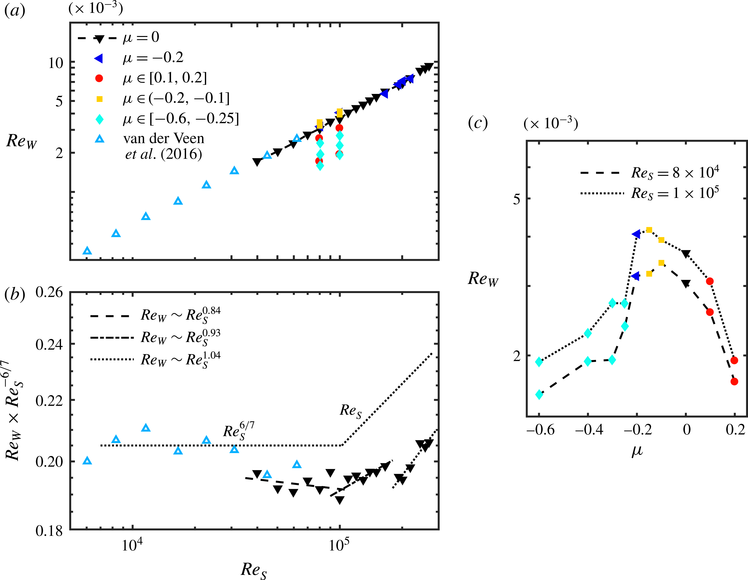
(a) Wind Reynolds number
 $Re_{W}$
based on the standard deviation of the radial velocity component
 $\unicode[STIX]{x1D70E}_{u_{r}}$
as a function of the shear Reynolds number
 $Re_{S}$
. The markers and colours separate the rotation ratio regimes, namely co-rotation (red circles), outer cylinder at rest (black downward-pointing triangles), low counter-rotation (yellow squares), rotation ratio of the torque maximum (blue triangles), high counter-rotation (cyan diamonds) and data taken from van der Veen et al. (Reference van der Veen, Huisman, Merbold, Harlander, Egbers, Lohse and Sun2016) for
 $\unicode[STIX]{x1D707}=0$
(open light blue triangles). (b) Wind Reynolds number as a function of the shear Reynolds number compensated by the classical regime scaling
 $Re_{S}^{\unicode[STIX]{x1D6FD}}$
with
 $\unicode[STIX]{x1D6FD}=6/7$
. The black lines represent least-squares fits in the classical, transitional and ultimate regimes:
 $Re_{W,CR}\sim Re_{S}^{0.84}$
(dashed),
 $Re_{W,TR}\sim Re_{S}^{0.93}$
(dash-dotted) and
 $Re_{W,UR}\sim Re_{S}^{1.04}$
(dotted). (c) Wind Reynolds number as a function of the rotation ratio
 $\unicode[STIX]{x1D707}$
for
 $Re_{S}=8\times 10^{4}$
(dashed line) and
 $Re_{S}=10^{5}$
(dotted line).

For pure inner cylinder rotation (
 $\unicode[STIX]{x1D707}=0$
) the wind Reynolds number is increasing with the shear Reynolds number and we find a nearly perfect agreement with the measurements of van der Veen et al. (Reference van der Veen, Huisman, Merbold, Harlander, Egbers, Lohse and Sun2016) in the lower
 $Re_{S}$
regime. According to Grossmann & Lohse (Reference Grossmann and Lohse2000, Reference Grossmann and Lohse2011) the wind Reynolds number scales as
 $Re_{W}\sim Re_{S}^{\unicode[STIX]{x1D6FD}}$
with
 $\unicode[STIX]{x1D6FD}=6/7$
in the classical and
 $\unicode[STIX]{x1D6FD}=1$
in the ultimate regimes. Therefore, in figure 15(b) also the wind Reynolds number compensated with the predicted scaling in the classical regime is shown. Focusing on our own data, we can assume three different scaling regimes. The first regime is valid up to
 $Re_{S}=10^{5}$
(
 $Ta=1.69\times 10^{10}$
) with a scaling exponent of
 $\unicode[STIX]{x1D6FD}=0.84\pm 0.07$
very close to the classical
 $\unicode[STIX]{x1D6FD}=6/7$
. Secondly, some kind of transition takes place with an exponent of
 $\unicode[STIX]{x1D6FD}=0.93\pm 0.05$
, before the last regime at
 $Re_{S}=2\times 10^{5}$
(
 $Ta=6.46\times 10^{10}$
) is reached with an exponent of
 $\unicode[STIX]{x1D6FD}=1.04\pm 0.08$
. The third one is in the range of the prediction for the ultimate regime. Although the exponents fit quite well to the expected ones, the significance of the results has to be considered carefully. We could only analyse a few partially scattered data points within the three mentioned regimes and the scaling seems not to be that strict especially when also including the data of van der Veen et al. (Reference van der Veen, Huisman, Merbold, Harlander, Egbers, Lohse and Sun2016). Further, we see a jump in between the second and third regimes, indicating that ultimate turbulence is still evolving. Nevertheless, we are confident that the close accordance with the predictions confirms the finding of the transition from classical to ultimate turbulence. Moreover, in figure 15(c) the wind Reynolds number is depicted over the rotation ratio
 $\unicode[STIX]{x1D707}$
. What can be observed here represents a similar behaviour to what was explained for the total kinetic energy with a maximum in the low counter-rotating regime for a rotation ratio slightly larger than
 $\unicode[STIX]{x1D707}_{max}$
.
4.2 Nusselt number
All investigations presented up to now were focused on the change in the flow field when the regime of the torque maximum is passed. Now, we want to analyse the angular momentum itself in terms of the Nusselt number. Therefore, we also use, next to the classical calculation according to (1.2) and (1.3) for the radial profiles of the quasi-Nusselt number, the flow field decomposition introduced in (3.8). Thus, the Nusselt number reads
 $$\begin{eqnarray}Nu_{\unicode[STIX]{x1D714}}=Nu_{\unicode[STIX]{x1D714}}^{turb}+Nu_{\unicode[STIX]{x1D714}}^{LSC},\end{eqnarray}$$
with its turbulent and large-scale circulation contributions
 $$\begin{eqnarray}\left.\begin{array}{@{}c@{}}\displaystyle Nu_{\unicode[STIX]{x1D714}}^{turb}=J_{lam}^{-1}\langle r^{3}\langle u_{r}^{\prime \prime }\unicode[STIX]{x1D714}^{\prime \prime }\rangle _{A(r),t}\rangle _{r},\\ \displaystyle Nu_{\unicode[STIX]{x1D714}}^{LSC}=J_{lam}^{-1}\langle r^{3}(\langle \bar{u}_{r}\bar{\unicode[STIX]{x1D714}}\rangle _{A(r),t}-\unicode[STIX]{x1D708}\unicode[STIX]{x2202}_{r}\langle \bar{\unicode[STIX]{x1D714}}\rangle _{A(r),t})\rangle _{r}.\end{array}\right\}\end{eqnarray}$$
Next to the mixed terms
 $\langle \bar{u}_{r}\unicode[STIX]{x1D714}^{\prime \prime }\rangle _{A(r),t}$
and
 $\langle u_{r}^{\prime \prime }\bar{\unicode[STIX]{x1D714}}\rangle _{A(r),t}$
, also
 $\unicode[STIX]{x2202}_{r}\langle \unicode[STIX]{x1D714}^{\prime \prime }\rangle _{A(r),t}$
vanishes, as they all are linear in the deviation quantities. There remain a Reynolds stress term in the turbulent part and a gradient term and the product of the averaged velocities in the large-scale circulation part. The last can be corrected assuming that the radial velocity vanishes when it is averaged across the whole measurement volume. The additional radial average of the decomposition products is necessary, as they depend on the radial location (see Brauckmann & Eckhardt Reference Brauckmann and Eckhardt2013b
). In figures 16 and 17 the radial profiles of the Nusselt number and the averaged value for different shear Reynolds numbers for
 $\unicode[STIX]{x1D707}=0$
are depicted.
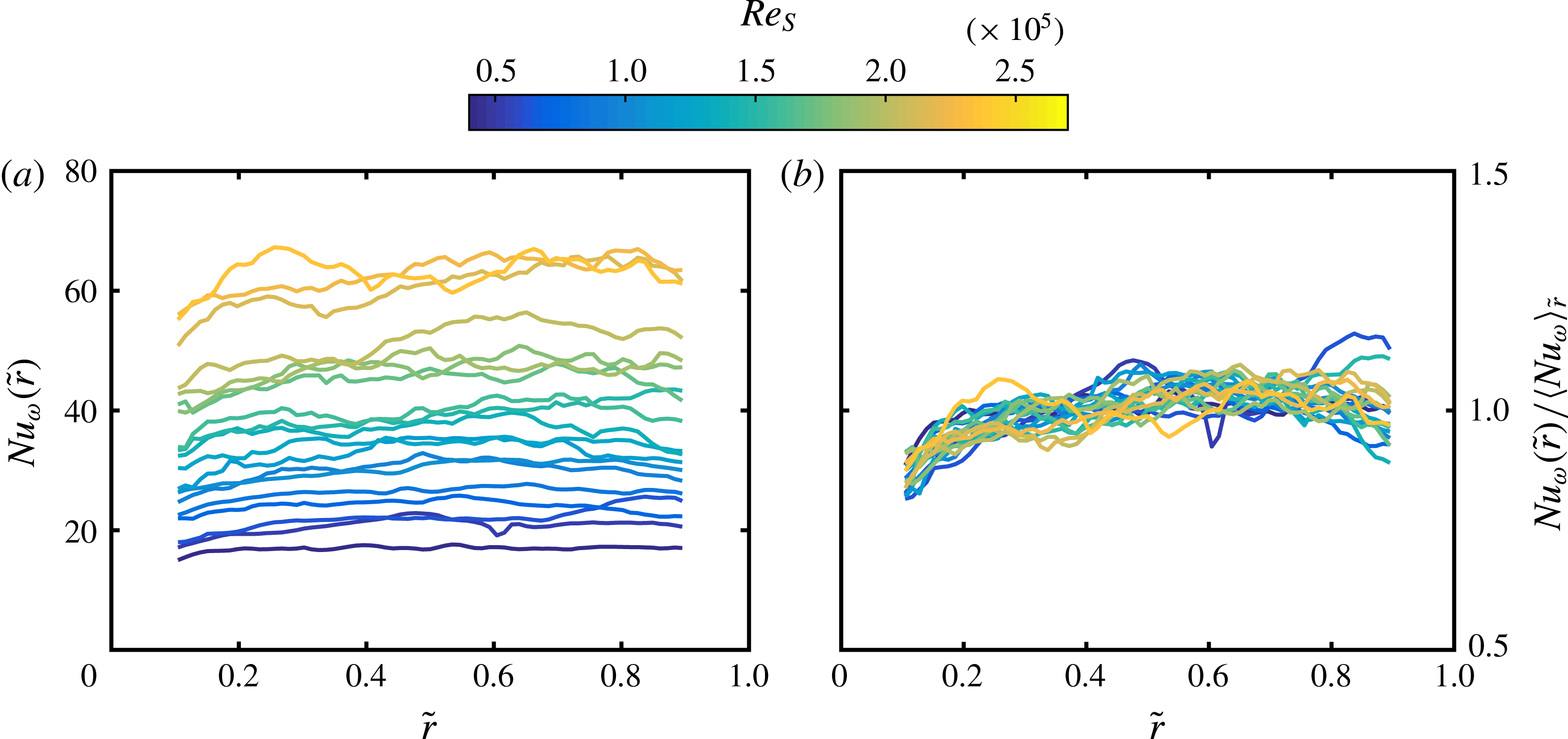
(a) Radial profiles of the Nusselt number
 $Nu_{\unicode[STIX]{x1D714}}(\tilde{r})$
calculated from the velocity field for different shear Reynolds numbers
 $Re_{S}$
for pure inner cylinder rotation (
 $\unicode[STIX]{x1D707}=0$
). (b) Radial profiles of the Nusselt number divided by its average value in the range of
 $\tilde{r}\in [0.1,0.9]$
. Discrete colours for the interpolated colour map are according to figure 7.

The Nusselt number is increasing with the shear Reynolds number and remains nearly constant for all radial positions, which is in good agreement with the definition of the angular momentum flux (see figure 16
a). In the region of the cylinder walls, the deviation of
 $Nu_{\unicode[STIX]{x1D714}}$
from a horizontal line increases. This becomes clearer when these profiles are divided by the radially averaged Nusselt number (see figure 16
b). Especially in the region of the inner cylinder, the profiles are below their average value, indicating a radially dependent underestimation. In the investigated
 $Re_{S}$
regime, the Reynolds stress term
 $\langle u_{r}^{\prime \prime }\unicode[STIX]{x1D714}^{\prime \prime }\rangle$
, which consists of the product of the velocity fluctuations, represents between 91 % and 99 % of the overall angular momentum flux in the fully turbulent regime for pure inner cylinder rotation. As the spatial resolution of the velocity measurements in the different horizontal planes is limited to 0.379–0.46 mm, these fluctuations are averaged over the corresponding grid. Further, the turbulent kinetic energy (see figure 11) is very large in the region of the inner cylinder at
 $\unicode[STIX]{x1D707}=0$
. Therefore the overall underestimation of the velocity fluctuations is pronounced in the inner gap region.
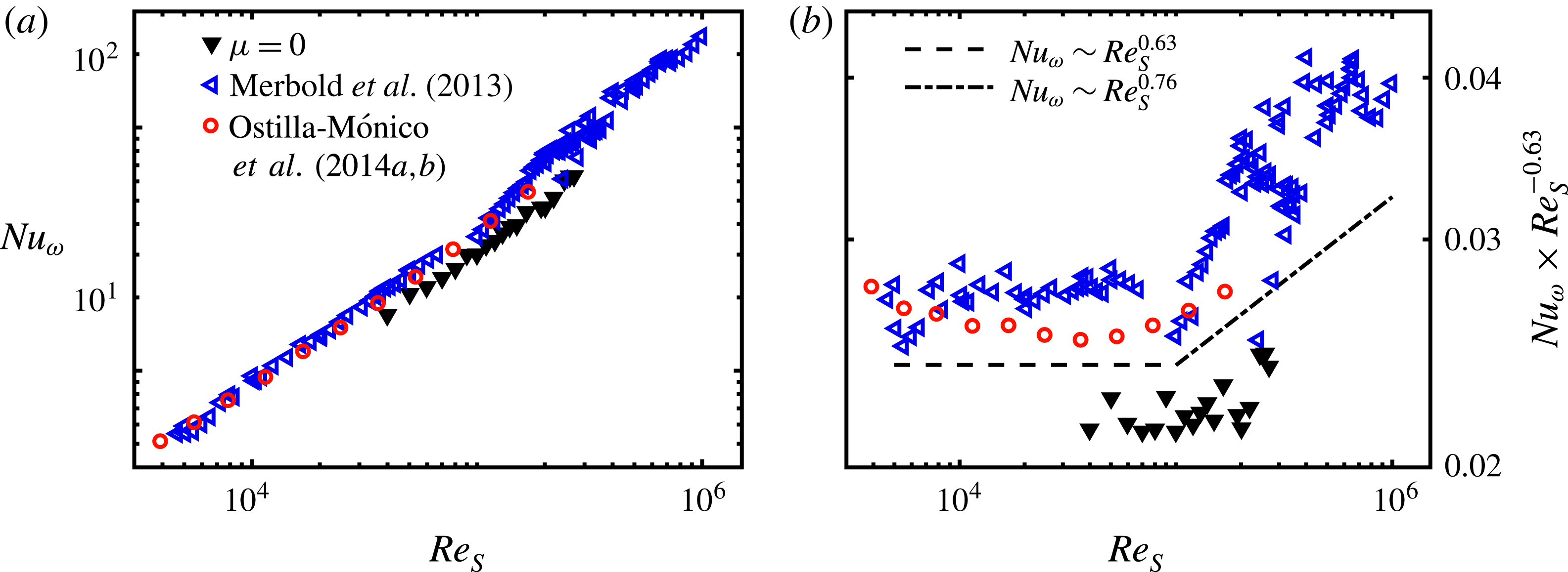
(a) Nusselt number
 $Nu_{\unicode[STIX]{x1D714}}$
averaged over the radial coordinate
 $\tilde{r}\in [0.1,0.9]$
as a function of the shear Reynolds number
 $Re_{S}$
for
 $\unicode[STIX]{x1D707}=0$
. Black filled triangles represent the values calculated from the PIV measurements. Blue open triangles are taken from the direct torque measurements of Merbold et al. (Reference Merbold, Brauckmann and Egbers2013) and red open circles from the numerical simulations of Ostilla-Mónico et al. (Reference Ostilla-Mónico, Huisman, Janninik, van Gils, Verzicco, Grossmann and Lohse2014a
,Reference Ostilla-Mónico, van der Poel, Verzicco, Grossmann and Lohse
b
) for comparison. (b) Nusselt number compensated by
 $Re_{S}^{-0.63}$
as a function of the shear Reynolds number. The dashed and dash-dotted lines indicate least-squares fits using our PIV data for the classical and ultimate regime with the power-law ansatz
 $Nu_{\unicode[STIX]{x1D714}}\sim Re_{S}^{\unicode[STIX]{x1D6FC}-1}$
and
 $Re_{S,c}=10^{5}$
:
 $Nu_{\unicode[STIX]{x1D714},CR}\sim Re_{S}^{0.63}$
and
 $Nu_{\unicode[STIX]{x1D714},UR}\sim Re_{S}^{0.76}$
.

The same effect is also visible in figure 17(a), where the PIV results are compared to the direct torque measurements of Merbold et al. (Reference Merbold, Brauckmann and Egbers2013) and the direct numerical simulations of Ostilla-Mónico et al. (Reference Ostilla-Mónico, Huisman, Janninik, van Gils, Verzicco, Grossmann and Lohse2014a
,Reference Ostilla-Mónico, van der Poel, Verzicco, Grossmann and Lohse
b
). The absolute values of
 $Nu_{\unicode[STIX]{x1D714}}$
are underestimated for all
 $Re_{S}$
, but are in the same order as the comparative data. Next to the restricted spatial and temporal resolution, here the small measurement volume compared to the whole TC volume also comes into account. Although it is not possible to clearly assign the most dominant reason for the underestimation, we can exclude differences induced by the wavelength of turbulent Taylor rolls, as their influence is negligible at pure inner cylinder rotation due to their low strength (see figure 5).
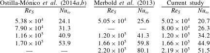
Comparison of Nusselt numbers for pure inner cylinder rotation between the numerical simulations of Ostilla-Mónico et al. (Reference Ostilla-Mónico, Huisman, Janninik, van Gils, Verzicco, Grossmann and Lohse2014a ,Reference Ostilla-Mónico, van der Poel, Verzicco, Grossmann and Lohse b ), the direct torque measurements of Merbold et al. (Reference Merbold, Brauckmann and Egbers2013) and our study.
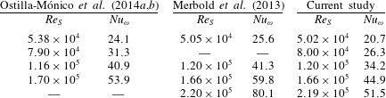
From table 4 we can see that the differences between the data of Merbold et al. (Reference Merbold, Brauckmann and Egbers2013) and our own measurements increase from
 $19\,\%$
at
 $Re_{S}=5\times 10^{4}$
to
 $36\,\%$
at
 $Re_{S}=2.19\times 10^{5}$
while those compared to Ostilla-Mónico et al. (Reference Ostilla-Mónico, Huisman, Janninik, van Gils, Verzicco, Grossmann and Lohse2014a
,Reference Ostilla-Mónico, van der Poel, Verzicco, Grossmann and Lohse
b
) stay more or less constant at approximately
 $16\,\%$
. The increase in the deviation with the shear Reynolds number is what one would expect, because with higher
 $Re_{S}$
the length and time scales of turbulent flows become smaller and, therefore, the error due to limited temporal and spatial resolution should increase. However, the direct torque data show partially stronger variations at specific
 $Re_{S}$
, which complicates the quantification of the differences.
Nevertheless, we can further compare the scaling exponent
 $\unicode[STIX]{x1D6FC}$
of the Nusselt number of our PIV data with those of the corresponding direct torque measurements and numerical simulations depicted. Here, it is important to note that
 $\unicode[STIX]{x1D6FC}$
depends on the shear Reynolds number
 $Re_{S}$
, reaching a nearly constant value not before
 $Re_{S}\approx 6\times 10^{5}$
(Merbold et al.
Reference Merbold, Brauckmann and Egbers2013). Owing to the small number of measurement points, it does not make sense within this study to calculate a local exponent. However, Merbold et al. (Reference Merbold, Brauckmann and Egbers2013) also reported an averaged exponent before and after the transition from the classical to the ultimate regime at approximately
 $Re_{S}\approx 10^{5}$
, which we use as comparison. In figure 17(b) the compensated Nusselt number reveals this change in scaling clearly for the direct torque data, but only blurred for our own measurements and the numerical ones. If we fit our data to a power-law ansatz, we find a scaling exponent of
 $\unicode[STIX]{x1D6FC}_{CR}=1.63\pm 0.11$
in the classical regime and
 $\unicode[STIX]{x1D6FC}_{UR}=1.76\pm 0.08$
in the ultimate regime, lying in the confidence intervals of
 $\unicode[STIX]{x1D6FC}_{Merbold,CR}=1.62\pm 0.04$
and
 $\unicode[STIX]{x1D6FC}_{Merbold,UR}=1.78\pm 0.06$
. In addition, in Ostilla-Mónico et al. (Reference Ostilla-Mónico, Huisman, Janninik, van Gils, Verzicco, Grossmann and Lohse2014a
,Reference Ostilla-Mónico, van der Poel, Verzicco, Grossmann and Lohse
b
) a scaling exponent of
 $\unicode[STIX]{x1D6FC}_{CR,Ostilla}\approx 1.66$
in the classical regime for
 $\unicode[STIX]{x1D702}=0.5$
and an exponent of
 $\unicode[STIX]{x1D6FC}_{UR,Ostilla}\approx 1.76$
independent of the radius ratio are reported. This good agreement between experimental data using different measurement techniques and numerical data is quite interesting, as the differences in Nusselt number should increase with
 $Re_{S}$
due to resolution limitations as explained before. One explanation might be the fact that a fixed scaling exponent is not yet reached in the shear Reynolds-number regime where our measurements have been performed. Also, the reported partially stronger variation in the direct torque data comes into account here.
The dependence of the Nusselt number on the rotation ratio is analysed based on the measurement data at
 $Re_{S}=10^{5}$
using the decomposition according to (4.2). In figure 18(a) the radial profiles of
 $Nu_{\unicode[STIX]{x1D714}}$
are depicted, showing a stronger radial deviation compared to the previous ones for
 $\unicode[STIX]{x1D707}=0$
. Further, in figure 18(b) the different fractions of the Nusselt number are plotted against the rotation ratio
 $\unicode[STIX]{x1D707}$
and compared with the direct torque measurements of Merbold et al. (Reference Merbold, Brauckmann and Egbers2013). Similar to the results of the energy distribution, the angular momentum transport due to the large-scale circulation is approximately zero for
 $\unicode[STIX]{x1D707}\geqslant 0$
and increases strongly in the low counter-rotating regime, with a pronounced maximum at
 $\unicode[STIX]{x1D707}=\unicode[STIX]{x1D707}_{max}$
. Its decrease for higher counter-rotation develops slower than observed for
 $\tilde{E}_{LSC}$
in figure 12. The plot for
 $Nu_{\unicode[STIX]{x1D714}}^{turb}$
exhibits a local and sharp minimum at
 $\unicode[STIX]{x1D707}_{max}$
and in summary the total Nusselt number maximizes at
 $\unicode[STIX]{x1D707}_{max}=-0.2$
. In comparison to the direct torque measurements of Merbold et al. (Reference Merbold, Brauckmann and Egbers2013), our
 $Nu_{\unicode[STIX]{x1D714}}$
values are larger for
 $\unicode[STIX]{x1D707}<0$
, where the large-scale fraction cannot be neglected, while at
 $\unicode[STIX]{x1D707}=0$
, the opposite holds. So, we can conclude that the turbulent fraction of the Nusselt number is underestimated, while the LSC fraction is overestimated, which is most pronounced at
 $\unicode[STIX]{x1D707}_{max}$
. This result enables a good insight into the evaluation of the angular momentum transport based on velocity fields. While a limited spatial resolution in the horizontal plane damps out velocity fluctuations, it over-rates the averaged secondary flow field mainly due to the more significant limited axial resolution. However, it is worth mentioning that the experimental data with which we are comparing result from different facilities, different measurement techniques and different endplate conditions, leading to possibly different vortex wavelengths. Thus, despite differences in the Nusselt number, the overall agreement between the total Nusselt numbers is quite good. The same decomposition of the Nusselt number for
 $\unicode[STIX]{x1D702}=0.5$
at a much lower Reynolds number of
 $Re_{S}=2\times 10^{4}$
has been done by Brauckmann & Eckhardt (Reference Brauckmann and Eckhardt2013b
), who found a much smoother changeover from an angular momentum transport dominated by turbulent fluctuations for
 $\unicode[STIX]{x1D707}>0$
to one dominated by large-scale circulations for
 $-0.6\leqslant \unicode[STIX]{x1D707}\leqslant -0.1$
and back again. This clearly shows that the rotation ratio range, where turbulent Taylor vortices can exist inside the gap, shrinks with increasing shear Reynolds number. It remains the question whether Taylor vortices can survive in the torque maximum region for infinite forcing.
(a) Normalized radial profiles of the Nusselt number
 $Nu_{\unicode[STIX]{x1D714}}(\tilde{r})$
calculated from the velocity field for the shear Reynolds number
 $Re_{S}=10^{5}$
and different rotation ratios. (b) Nusselt number
 $Nu_{\unicode[STIX]{x1D714}}$
(blue triangles) decomposed into its large-scale (yellow squares) and turbulent (red circles) contributions, which are averaged over the radial coordinate, as a function of the rotation ratio
 $\unicode[STIX]{x1D707}$
for
 $Re_{S}=10^{5}$
. Cyan open diamonds represent the direct torque measurement data taken from Merbold et al. (Reference Merbold, Brauckmann and Egbers2013) for reference.

5 Conclusion
In this paper we have presented an axial exploration of a wide-gap TC flow at high shear Reynolds numbers using PIV in horizontal planes at different cylinder heights to analyse the flow structure for co- and counter-rotation. Special attention was paid to the region of maximum transport of angular momentum in the low counter-rotating regime (
 $\unicode[STIX]{x1D707}=\unicode[STIX]{x1D707}_{max}$
), where turbulent Taylor vortices are formed in the gap. We could show that these vortices are statistically stable in time, which makes deeper investigations possible. To verify the prediction for the torque maximum according to Brauckmann & Eckhardt (Reference Brauckmann and Eckhardt2013b
), we investigated the angular velocity and angular momentum profiles in the bulk, finding the smallest radial gradient of angular velocity and the start of the detachment of the neutral surface from the outer cylinder wall coinciding with
 $\unicode[STIX]{x1D707}_{max}$
. While these findings are in good agreement with those of van Gils et al. (Reference van Gils, Grossmann, Sun and Lohse2012) and Ostilla-Mónico et al. (Reference Ostilla-Mónico, Huisman, Janninik, van Gils, Verzicco, Grossmann and Lohse2014a
), they contradict the studies of Ostilla et al. (Reference Ostilla, Stevens, Grossmann, Verzicco and Lohse2013) and Brauckmann et al. (Reference Brauckmann, Salewsky and Eckhardt2016). In our opinion these differences result from differences in the investigated shear Reynolds-number regimes. As our results are only less dependent on
 $Re_{S}$
, we are convinced that investigations at high shear Reynolds number are needed to reveal general flow behaviours. Further, we detected a shape similarity between the laminar Couette solution and fully turbulent bulk profiles for
 $\unicode[STIX]{x1D707}\geqslant 0$
, which calls for additional investigations in the future.
In a next step we decomposed the velocity field into its large-scale and turbulent contributions and calculated the corresponding kinetic energy fractions. Here, we found a maximum of the large-scale circulation energy and a local minimum of the turbulent kinetic energy at the rotation ratio of the torque maximum. This clearly shows the increase of coherence in the flow at
 $\unicode[STIX]{x1D707}=\unicode[STIX]{x1D707}_{max}$
. Furthermore, while the growth of turbulent Taylor vortices takes place in a continuous process, their breakdown occurs suddenly. Unexpectedly, the sum of both energy fractions maximizes at a slightly larger rotation ratio than
 $\unicode[STIX]{x1D707}_{max}$
. Moreover, we calculated the wind Reynolds number for different rotation ratios, showing that it is necessary to include also the axial dispersion into the standard deviation of the wind velocity. For pure inner cylinder rotation, we could identify the beginning of the transition from the classical to the ultimate turbulent regime at
 $Re_{S}=10^{5}$
based on its scaling exponent in accordance with Huisman et al. (Reference Huisman, van der Veen, Sun and Lohse2014) and van der Veen et al. (Reference van der Veen, Huisman, Merbold, Harlander, Egbers, Lohse and Sun2016). Interestingly, the change of
 $Re_{W}$
with the rotation ratio is similar to the one found for the total kinetic energy with a maximum located at
 $\unicode[STIX]{x1D707}$
slightly larger than
 $\unicode[STIX]{x1D707}_{max}$
.
In the end, we also analysed the Nusselt number, finding a blurred change in the scaling exponent with the shear Reynolds number again at
 $Re_{S}=10^{5}$
and values of the scaling exponent close to those of Merbold et al. (Reference Merbold, Brauckmann and Egbers2013) and Ostilla-Mónico et al. (Reference Ostilla-Mónico, Huisman, Janninik, van Gils, Verzicco, Grossmann and Lohse2014a
,Reference Ostilla-Mónico, van der Poel, Verzicco, Grossmann and Lohse
b
). In addition we used the former introduced flow field decomposition, finding a maximum of
 $Nu_{\unicode[STIX]{x1D714}}^{LSC}$
and a local minimum of
 $Nu_{\unicode[STIX]{x1D714}}^{turb}$
at the rotation ratio of the torque maximum. In comparison to the results of Brauckmann & Eckhardt (Reference Brauckmann and Eckhardt2013b
), the range of rotation ratios, where turbulent Taylor vortices can exist, shrinks strongly with the shear Reynolds number.
In conclusion, this study revealed some new insights into a wide-gap TC flow in the fully turbulent regime around the vortex-dominated torque maximum region.
Acknowledgements
We gratefully acknowledge financial support by the DFG FOR 1182 (EG100/15-2). Also, we would like to thank B. Eckhardt and A. Shahirpour for helpful comments and E. Pascu for experimental assistance.