

Introduction
China has achieved remarkable progress in poverty alleviation in just a few decades. According to the World Bank, the poverty headcount ratio at 1.90 US dollar per day (2011 Purchasing Power Parity, or PPP) decreased from 66.6 per cent in 1990 to 1.9 per cent in 2013. The statistics from the National Bureau of Statistics of China (NBSC) (2015) consistently show that the rural population in poverty has reduced from 770 million in 1978 to 70 million in 2014 based on the poverty line set by the Chinese government, i.e. annual individual income of Chinese yuan (CNY) 2,300.
When assessing poverty, income has been pervasively adopted as the main, if not the only, criterion. While income may be easier to record, its use may not be desirable in China due to its lack of reliability and validity. First, income can fluctuate significantly even when measured at an annual scale. Not everyone, particularly the poor population, has stable jobs, and this could be exaggerated by an economic downturn. In addition, it is evident that more and more young people choose to be freelancers and experience unstable earnings (Zheng, Reference Zheng1994). Furthermore, agriculture is severely influenced by weather and other uncontrollable conditions. Therefore, the income of rural residents, to which agriculture can make a primary contribution, can be unstable. Second, income, as a flow of wealth, cannot capture the full economic status. One primary component left out is accumulated wealth, i.e. assets, so the poverty estimated by income can be biased. In sum, income-based poverty cannot offer a comprehensive description of poverty for the Chinese population.
The situation described above can also be seen outside China. According to Caner and Wolff (Reference Caner and Wolff2004), the US asset-poverty rate was two to four times higher than the income-poverty rate in 1999, and the gap was generally consistent from 1984 to 1999. A similar pattern was found in Canada, Finland, Germany, Italy, Norway, Sweden and the UK; the asset-poverty rates were two to three times the income-poverty rates in those countries in 2000 (Brandolini et al., Reference Brandolini, Magri and Smeeding2010).
Thus, assets could be at least a comparable, if not better, alternative measure, as assets are less likely to have the two possible flaws of income-based measures. Assessing assets can additionally evaluate the economic ability to 1) guard against economic hardship, as people would cash in their assets to ameliorate declining consumption; and 2) achieve individual and family development goals, as funding many kinds of these goals – for example, higher education and microenterprise – requires an amount of money more than the total income of many months (McKernan and Sherraden, Reference McKernan and Sherraden2008; McKernan et al., Reference McKernan, Ratcliffe and Vinopal2009). Moreover, the earnings from assets may constitute a significant proportion of a person’s wealth (Miranda-Agrippino and Rey, Reference Miranda-Agrippino and Rey2014).
This paper documents a study describing the economic well-being of Chinese people in both rural and urban areas. By introducing the concept of asset poverty and using the most recent wave of Chinese Household Income Project data, the research aimed at 1) reporting poverty status in both urban and rural China, 2) describing demographic characteristics of asset-poor households, and 3) identifying challenges and possible solutions for poverty alleviation in China.
Background
The effects of assets
Michael Sherraden was among the first to articulate an asset-based approach to poverty alleviation. His key insights include that assets matter economically, socially and psychologically in ways that income alone does not (Sherraden, Reference Sherraden1991). Recent research conducted in the United States illustrates that income itself is not sufficient to allow families to escape poverty, achieve financial stability and move up the economic ladder.
Mckerman et al. (Reference McKernan, Ratcliffe and Vinopal2009) showed that savings and assets were correlated with low-income families’ ability to weather unexpected employment gaps and hardships related to health care and housing payments, food security, and basic consumption. They found that households with at least $2,000 in liquid assets were less likely to forgo visits to the doctor or miss utility payments, compared with those with fewer or no assets. McKernan et al. (Reference McKernan, Rademacher, Ratcliffe, Wiedrich and Gallagher2011) confirmed that low-income homebuyers who purchased a home with the help of an Individual Development Account were two to three times less likely to lose their homes to foreclosure.
Assets also have crucial effects on education, which serves as a cornerstone for development. Zhan and Sherraden (Reference Zhan and Sherraden2003) showed that children in families with as little as $3,000 in savings had been found to have greater odds of graduating from high school than children in families without savings. Assets also can increase the likelihood of going to and succeeding in college. Elliott and Beverly (Reference Elliott and Beverly2011) presented that children with savings dedicated to college education were four times more likely to attend college than children without such savings. Also, among youths who expect to attend college, those with a savings account in their names are roughly seven times more likely to actually attend, compared to those without this kind of savings accounts (Elliott and Beverly, Reference Elliott and Beverly2011). Zhan and Sherraden (Reference Zhan and Sherraden2009) concluded that savings and other financial assets were consistent predictors of college graduation, even after controlling for variables such as income.
In addition, a handful of studies have shown that the ownership of assets can promote success in the labour market. Lerman and McKernan (Reference Lerman and McKernan2008) suggested that financial assets and car ownership were correlated with positive income and employment outcomes. A one-percent increase in wealth was found to provide a five-percent increase in the likelihood that young men will avoid low-wage jobs (Morillas, Reference Morillas2007). Bynner and Despotidou (Reference Bynner and Despotidou2001) showed that savings at age 23 resulted in lower unemployment between ages 23 and 33.
Assets can also enhance the well-being and life chances of children and youths. Shanks (Reference Shanks2007) found that household wealth was positively associated with children’s cognitive and behavioural development. Homeownership is positively associated with decreased teenage pregnancy and decreased behavioural problems (Green and White, Reference Green and White1997).
In conclusion, assets, as a resource, improve quality of life via the ability to acquire ‘savings, education, good health, home ownership, and the connections people have to each other as pathways or networks to other resources and mutual support’ (IASP, Brandeis University). In other words, assets are relevant to individual empowerment, as claimed by Sen (Reference Sen1997). Further, the impact of assets can be persistent across generations compared with income, because the value of assets remains steadfast against economic change and assets are inheritable (Nam et al., Reference Nam, Huang, Sherraden, McKernan and Sherraden2008).
Asset poverty
Households are defined as asset poor if their access to asset-type resources is insufficient for meeting basic needs for a period of three months based on the estimated duration of unemployment (2.2–4.2 months) which is a common event resulting in economic hardship (Caner and Wolff, Reference Caner and Wolff2004; Haveman and Wolff, Reference Haveman and Wolff2005). Basic need is measured by the household-size conditioned poverty threshold (Citro and Michael, Reference Citro and Michael1995). Net worth, minus home equity and liquid assets are usually used to measure asset-type resources. Haveman and Wolff (Reference Haveman and Wolff2001) and Caner and Wolff (Reference Caner and Wolff2004) defined net worth as the sum of all marketable assets less the value of all debts, and liquid assets as the value of cash and other kinds of easily monetisable asset items.
Asset poverty provides another perspective of viewing poverty. For instance, even though income poverty rates in the United States had improved from 1983 to 2001, net-worth poverty rates had risen from 22.4 per cent in 1983 to 24.5 per cent in 2001 while liquid-asset poverty rates had also increased from 33.2 per cent to 37.5 per cent (Haveman and Wolff, Reference Haveman and Wolff2005). Another study indicated asset poverty rates did not parallel income poverty rates in Canada and the developed countries in Europe (Brandolini et al., Reference Brandolini, Magri and Smeeding2010). In urban China, a similar pattern has been reported. The liquid asset-poverty rate was five times the income-poverty rate in 2002 (Huang et al., Reference Huang, Jin, Deng, Guo, Zou and Sherraden2013). All of the findings showed that asset poverty could unveil another aspect of material hardship other than income poverty.
Empirical studies confirmed that asset poverty was associated with several demographic characteristics of households in the US (Aratani and Chau, Reference Aratani and Chau2010; Bucks et al., Reference Bucks, Kennickell and Moore2006; Haveman and Wolff, Reference Haveman and Wolff2001, Reference Haveman and Wolff2005). Households headed by African Americans, people with low education attainment, or renters, or households with children and/or the elderly were more likely to be in asset poverty. Studies in other countries generally reported the same associations (Cheng, Reference Cheng2008; Huang et al., Reference Huang, Jin, Deng, Guo, Zou and Sherraden2013; Naschold, Reference Naschold2012).
Poverty in China
Since the pro-market reforms in 1978, China has achieved astonishing economic growth. For roughly the first three decades following the reform, China kept an average annual GDP growth of 9 per cent (World Bank, 2006). Different estimates have been made regarding the number of people that were lifted out of poverty during this time, ranging from 250 million (ADB Poverty Analysis China, 2010) to 400 million (World Bank, 2006).
However, in the early 1990s, new policies helped initiate the creation of a group of urban poor. The pro-market reform process led to the bankruptcy of many state-owned and collective enterprises in an attempt to improve productivity and efficiency among these firms (NBS China Labor Statistical Yearbook, 2005). This resulted in a massive unemployment rate in urban China, as well as low wages, inadequate pensions, and rampant inflation (Saunders and Shang, Reference Saunders and Shang2001). The number of laid-off workers from state-owned enterprises was 5.9 million in 1998 (NBS China Labor Statistical Yearbook, 2005). Eighty-three million people lived under the World Bank’s $1 per day per capita poverty line and over 200 million of them were below the $1.25 per day per capita poverty line by the end of 2013 (State Council of China, 2014).
Moreover, it’s also worth noticing that the distribution of poverty in China is unbalanced in terms of geography. The vast majority of poor people are from rural China and most of them reside in western regions, such as the provinces of Yunnan and Guizhou. In contrast, urban residents in eastern regions share the smallest proportion of the poor in China. Recognising these growing issues of new-wave poverty and inequality, the China Central Government set up a new poverty reduction goal in 2015: that absolute poverty will be eradicated by 2020 (Xinhua News Agency, 2015).
The Minimum Living Standard (MLS) Assistance (MLSA) programme, the major welfare programme against poverty after the pro-market reform, was first launched by the government in several cities in the early 1990s and expanded to all cities in 1999 (Gao and Riskin, Reference Gao, Riskin, Davis and Wang2009; Tang, Reference Tang2005). The amount of MLSA beneficiaries rose from 0.89 million in 1997 to 2.66 million in 1999 (Gao et al., Reference Gao, Garfinkel and Zhai2009). In 2003, the state began to establish the rural MLSA. 2,037 counties from 15 provinces adopted the rural MLSA programme in the same year, targeting 4 million rural poor residents (Tang, Reference Tang2005). However, there were huge gaps between urban and rural areas with regard to the level of assistance provided by MLSA. This unequal situation did not change until 2015. Shanghai became the first city to make the urban and rural MLSA uniform and then many coastal cities followed.
The MLS line (monthly amount per capita in CNY) is set by local governments following general guidelines from the central government. Basically, the MLS line should be calculated according to the local minimum living standard, which is based on local average per-person income and basic consumption needs including food, clothing and shelter, taking into consideration utilities, medical care and tuition expenses (Tang, Reference Tang2005). It is adjusted annually based on local social and economic development, as well as inflation (Tang, Reference Tang2005).
Method
Data
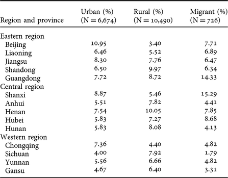
The study used the data yielded by the 2013 urban, rural and migrant household survey of CHIP, which is the most recent wave. It is a repeated cross-sectional national research administered by the scholars at Beijing Normal University and other universities across different countries, with assistance from the National Bureau of Statistics of China. To ensure national representativeness, CHIP adopted a sub-sample from the annual integration household survey of NBSC, applying the systematic sampling method. The CHIP survey captures the information of 7,175 urban households, 11,013 rural households, and 760 migrant households, which covers provinces from eastern, central and western regions of China. Table 1 below shows the respective sample size and geographical affiliation of the 14 provinces. CHIP is widely considered to be one of the best available databases, which provides full information on household income, assets and other related variables in China (Gustafsson et al., Reference Gustafsson, Li and Sicular2008).
Data by provinces

For urban samples, nearly 40 per cent of the families are in eastern provinces like Beijing and Guangdong, and approximately 34 per cent of them reside in central China. Regarding the rural households in the data, 35 per cent of them live in an eastern region and 39 per cent reside in central China. And, for the migrant households, 42 per cent of them are in eastern China and 40 per cent are in central China. So, in general, households were evenly sampled from the eastern, middle and western parts of China.
Measures
Asset poverty
According to Haveman and Wolff (Reference Haveman and Wolff2001), a household would be considered to be in asset poverty if the value of their assets could not meet basic needs for three months, and the study treated poverty line as a proxy of basic needs. In this study, household assets were measured in liquid assets, which is the wealth readily available for cashing in – for example, the balance in current and saving accounts, stocks, bonds, shares, etc; as CHIP 2013 does not provide any information of other assets on a continuous scale.
Considering the Chinese context, six different poverty lines were used for the purpose of comparison and sensitivity test: three lines of 1.25, 1.9 and 2 US dollars per day per capita used by the World Bank; the official poverty line of MLS in 2013 set by local governments for rural and urban areas respectively; and the poverty line reported by each household available in the dataset (referred to as the self-reported line in the rest of the paper).
The poverty line of $1.25 per day per capita was set up based on the average poverty standard among the 15 poorest countries in 2008 and was adjusted by PPP index (Haughton and Khandker, Reference Haughton and Khandker2009). This is the extremely-poor line for all countries and was updated to $1.9 in 2015 (State Council of China, 2014). The $2 poverty line is the moderate-poor standard established in 2008 by the World Bank (Haughton and Khandker, Reference Haughton and Khandker2009). Given that the $2 line is very close to the $1.9 line, sensitivity tests were performed and found the results yielded according to the two lines were consistent. Therefore, the paper does not provide the results using the $2 line, though they are available upon request. The exchange rate between US dollars and Chinese currency in 2013, 6.196, was used when presenting the results (World Bank, 2014).
Other measures
The variables used to predict asset poverty included household income, household location, family structure and demographic characteristics of household heads. The family structure was measured by household size, whether any people with disability were present, whether any elderly family members were present, and the number of non-adult children. The demographics of household heads included sex (female or male), age in years, education in years, ethnicity (Han or minority), political party (Communist or other), marital status (married or not), employment situation (employed or not) and health condition (healthy or not).
Analysis
Univariate and bivariate analyses were launched to describe the sample including the demographics, the poverty rates and whether covered by any social welfare programmes. Logistic models then separately predicted asset poverty according to the urban MLS line and the rural MLS line respectively by the demographics of households and household heads. As migrant households were either rural families living in urban areas or vice versa, they were included in both regressions to be compared with the urban sample or rural sample. Finally, according to the two World Bank lines and self-reported lines, the full sample containing urban, rural and migrant households was analysed to study the association between demographics and asset poverty.
Results
Characteristics of demographics and poverty
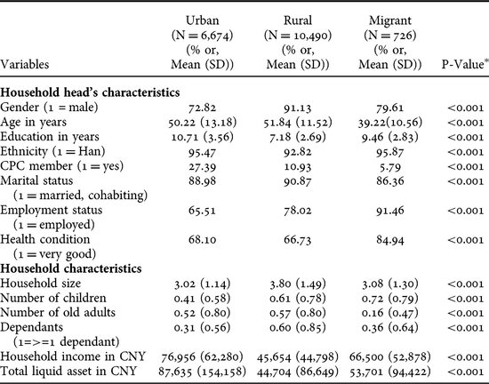
Table 2 summarizes and compares the demographic characteristics among urban, rural and migrant households. Overall, the majority of household heads tend to be middle-aged married Han males among the full sample. The average education attainment for urban household heads was high school, compared with middle school for migrant householders and primary school for rural householders (F = 2,707, p<. 001). About 27 per cent of the urban householders were members of the Communist Party of China (CPC), whereas much smaller proportions of rural and migrant household heads joined CPC (11 per cent and 6 per cent respectively) (χ2 = 853, p<. 001). The employment rate of 65.51 per cent for urban household heads was far behind its counterparts, with over 90 per cent for migrant household heads and 86 per cent for rural household heads (χ2 = 452, p<. 001). Migrant family heads reported a higher proportion of good health condition than urban and rural family heads (χ2 = 85, p<. 001).
Sample characteristics by urban, rural and migrant households

Note: P value of Chi-square test or ANOVA to test the differences among the three groups.
On average, urban families had the smallest number of children and dependants among the three groups (0.41 and 0.31 respectively). Migrant households had, on average, 0.72 children, which was the most among the three groups. The number of dependants in rural families was twice as many as in urban households. Regarding household income, the urban group was the richest (M = $12,420, Standard Deviation [SD] = $10,052), the second was migrant families (M = $10,733, SD = $8,534), and the poorest was the rural group (M = $7,368, SD = $7,229 yuan) (F = 736, p<. 001). Household liquid assets follow the same rank. On average, urban families held liquid assets of 14,144 US dollars (SD = $24,880), followed by migrant households with 8,867 dollars (SD = $15,239) and rural households with 7,215 dollars (SD = $14,307) (F = 261, p<. 001).
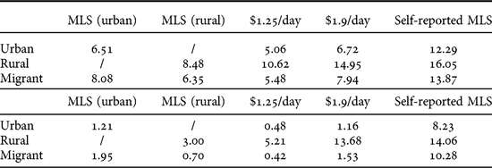
Table 3 presents the asset-poverty rate and the income-poverty rate for the urban, rural and migrant households according to the MLS line, the two World Bank lines and the self-reported line. Overall, the rural households had the highest poverty rate, followed by the migrant households, and the urban group had the lowest poverty rate regarding both asset poverty and income poverty across all the criteria. The self-reported line set the high criterion, which yielded the highest proportion of asset-poor population. Generally, the World Bank $1.25 line generated a slightly lower poverty rate in both urban and migrant households under MLS while, for rural families, the $1.25 line yielded a 2 per cent higher asset poverty rate than rural MLS. Under the World Bank $1.9 poverty line, 15 per cent of the rural households suffered from asset poverty and 14 per cent were categorized as income-poor as well. This was approximately the same as the highest poverty rate generated by the self-reported line. The rates of income poverty also followed a similar trend, but they were up to ten times lower than the asset-poverty rates under all the poverty lines. For example, according to the urban MLS line, less than 2 per cent of urban and migrant people were classified as income-poor, while the rates of asset poverty were at least 6 per cent.
Comparing asset poverty rate to income poverty rate under different poverty lines (The upper half of the table is the asset poverty rate; the bottom half is the income poverty rate)

Note: Sensitivity test between World Bank $2/day and $1.9 was conducted and no statistical significance was found. The result based on $2/day is available upon request.
Who are the asset-poor?
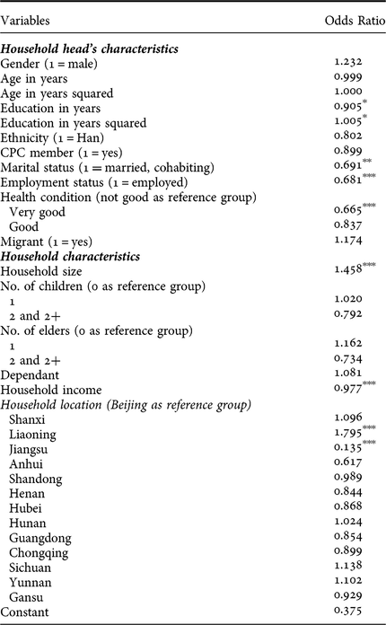
The logistic regression was adopted to describe the characteristics of the urban and migrant asset-poor based on the urban MLS line. A curve relationship was found between education and asset poverty. Below junior high school, the education of household heads is positively related to asset poverty whereas, above that, more education years is associated with lower odds of falling into asset poverty. Households with an unmarried or unemployed head were significantly predictive of falling into liquid asset poverty. Being in good health was, as expected, negatively associated with asset poverty for both urban and migrant households. Each additional unit increase in the household size was associated with 46 per cent higher odds of asset poverty in urban regions. Unsurprisingly, households with a low household income were more likely to be asset-poor than others living in urban China.
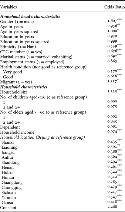
Table 4 summarises the relationship between household demographics and asset poverty for the rural and migrant sample, according to the rural MLS line. The results were generally consistent with the urban results in Table 5. Having a household head who is a minority, or in fair or even bad health was strongly predictive of getting trapped in asset poverty. Households with a married or female household head had lower odds of being in asset poverty. In addition, the membership of CPC was associated with lower odds of being in asset poverty in rural China. Household size and income were still significant predictors of asset poverty. Having a migrant household head was associated with 36 per cent higher odds of liquid asset poverty. Moreover, geographic location became a strong predictor for asset poverty in rural China. More specifically, using Beijing as the reference, families in most of the other provinces had lower odds of asset poverty. Predictors like education and employment status were no longer statistically significant.
Predicting asset poverty for rural and migrant households using the rural MLS line (N = 10,282)

*** p<0.01, ** p<0.05, * p<0.1
Predicting asset poverty for urban and migrant households using the urban MLS line (N = 6,936)

*** p<0.01, ** p<0.05, * p<0.1
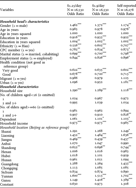
Table 6 presents the results for the full sample using the World Bank lines and the self-reported line. Education, ethnicity, marital status, gender, employment, health condition, CPC membership, household size, household income and household location were again significant predictors of asset poverty across all the poverty lines. Migrant status, which is a significant predictor for the rural and migrant sample according to the rural MLS line, was no longer statistically significant.
Predicting asset poverty for full sample using the World Bank lines and the self-reported line

*** p<0.01, ** p<0.05, * p<0.1
Income poverty, asset poverty, and public assistance
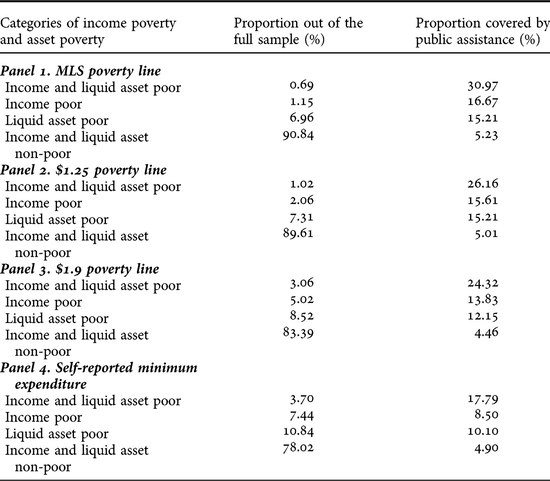
The sample was classified into four groups according to the poverty status: the income-and-asset poor, the income poor only, the asset poor only, and the income-and-asset non-poor. The income-poor-only group possessed assets above the asset-poverty line, while the income of the asset-poor-only group was above the income-poverty line.
According to the MLS lines (Panel 1 in Table 7), 0.69 per cent of households were both income- and liquid-asset poor. This group was the most vulnerable, but just 31 per cent of them received some kind of public assistance. Of the sample, 1.15 per cent were experiencing income poverty only, and approximately 17 per cent of households in that group received public assistance. Combining the first and second groups, about half of income-poor households were asset-poor. The rate was similar to that in Norway, the UK, and Sweden, but much higher than other developed countries reported in Brandolini et al. (Reference Brandolini, Magri and Smeeding2010). Seven per cent of households were asset-poor-only. About 17 per cent of households in this group received public assistance. Similar trends were found in other panels that used the World Bank $1.25 poverty line, the World Bank $1.9 poverty line, and the self-reported minimum living standard, respectively. In sum, a fairly low coverage of public assistance was reported for poor households regardless of the poverty lines.
Poverty and public assistance coverage

Discussion
Asset poverty and household demographics
The rate of asset poverty measured by liquid assets decreased from 17 per cent in 2002 (Huang et al., Reference Huang, Jin, Deng, Guo, Zou and Sherraden2013) to 6.5 per cent in 2013 referring to the urban MLS line, while the rate of income poverty decreased from 3.3 per cent (Huang et al., Reference Huang, Jin, Deng, Guo, Zou and Sherraden2013) to 1.2 per cent. Given that the urban MLS line in 2013 was higher than that in 2002, the reduction in both asset poverty and income poverty is prominent. Nevertheless, the gap between asset poverty and income poverty noticeably stayed at five times (2002: 17 per cent/3.3 per cent=5.1; 2013: 6.5 per cent/1.2 per cent=5.4).
Consistent with previous findings (Jalan and Ravallion, Reference Jalan and Ravallion2000), health condition, marital status, household income and household size were significantly associated with the likelihood of being asset poor in both urban and rural China, and higher household income, as expected, had a negative relationship with asset poverty. A ‘U’ shape of age was found in the relationship with asset poverty for the rural and migrant sample when using the rural MLS line. This might be because, as household heads mature, the working experience and asset accumulation tend to be enhanced; hence, they are less likely to be asset-poor (Paglin, Reference Paglin1977). However, after a certain age, either the marginal return of their working experience starts to decline or they could be pushed out of the job market, both of which can cause negative asset accumulation.
Although poverty may feature both as a cause and consequence of ‘male absence’, female-headed households in rural China surprisingly had lower odds of falling into asset poverty. Baden (Reference Baden1999) summarised that women might actively choose headship as a means by which they are able to enhance the well-being of their households and/or exert more control over their own lives. That could be the case in rural China. Female household headship might indicate an obvious financial advantage over male members in her household but not necessarily the absence of a male. This kind of household, therefore, is likely to have more sources of earnings. Other research also suggests that members of female-headed units are not necessarily worse-off than their counterparts in male-headed households (Chant, Reference Chant1997).
This study showed that leading by a minority head is associated with a higher asset poverty possibility for the rural and migrant households. Du et al. (Reference Du, Park and Wang2005) and Tong and Wang (Reference Tong and Wang2006) argued that the economic disadvantage of minority household heads was mainly due to the lag of regional development, as most minority populations live in western China which is economically less-developed. However, in this paper, the relationship between asset poverty and ethnicity was still significant after controlling for household demographics and regions. This might indicate that other reasons associated with ethnicity, such as culture and languages, could contribute to asset accumulation.
These three variables, age, gender and ethnicity, plus CPC membership, were only significant in the rural panel (the rural and migrant households) based on the rural MLS line, but not in the urban panel (the urban and migrant households) based on the urban MLS line. As the rural MLS line, $4.32 per day per household, was much lower than the urban MLS line, $6.64 per day per household, it implies that the difference in assets due to either variable is small, which is only influential at a low poverty line.
In contrast, education was significant to asset poverty in the urban panel, but not in the rural panel. There are two possible explanations. First, educational attainment of rural Chinese could be too low to achieve personal development. According to our data, the average educational attainment in China was only seven years, which was even lower than the rest of Asia in the 1990s (Psacharopoulos, Reference Psacharopoulos1994). Second, the average return of education in rural China was found to be lower than five per cent (Meng, Reference Meng1996; Parish et al., Reference Parish, Zhe and Li1995; Zhao, Reference Zhao1999), compared to that in the developing world, which was over 10 per cent, and in other Asian countries, which exceeded nine per cent (Psacharopoulos, Reference Psacharopoulos1994). Incidentally, since most rural residents are self-employed doing farm work, this may make employment insignificant in terms of predicting the rural asset poor.
Migrant households
Based on the Push and Pull theory, Cui (Reference Cui2009) reported two main pull factors for migrant workers to work in cities: economic motivation and more career opportunities. With rapid economic development and urbanisation in China, more working opportunities in labour-intensive industries, as well as in service industries, are becoming available in urban areas. On the other hand, push factors offered by rural places include low disposable income, underdeveloped infrastructure and underdeveloped healthcare provision, which motivate young or educated rural residents to move out. In China, migration to cities has played an essential role in poverty reduction (Ravallion and Chen, Reference Ravallion and Chen2007; Yao, Reference Yao2000). The average annual income of migrant workers increased by CNY 8,738 after moving to cities, and 20 per cent of them even earned CNY 10,000 more than what they had in rural areas (Li, Reference Li2003).
The result yielded by the univariate analysis was consistent. As Table 3 shows, the migrant families had similar rates of both income poverty and asset poverty, and were much better than their rural counterparts under all the criteria. For instance, based on the World Bank $1.9 line, the income poverty rate of the urban households and the migrant households were 1.2 per cent and 1.5 per cent, while the rate of the rural households were nearly 14 per cent. The rates of asset poverty of the two former groups were also close, 8 per cent and 6.7 per cent respectively, and much lower than that of the rural sample, i.e. 15 per cent.
However, the multivariate analysis revealed that migration predicted higher odds of asset poverty after controlling for household demographics. That is to say, migrant families could be better off in terms of income while they might still be struggling with asset poverty, possibly because the improvement in income had not been transferred to a significant accumulation in assets. Moreover, the next generation might continue to suffer from income poverty and asset poverty since their asset accumulation is inadequate to support sustainable personal development. However, as the data are cross-sectional, the analysis cannot exclude reverse causation, which is that conquering asset poverty motivates migration.
Asset poverty and geographic difference
The literature on regional inequality and rural poverty is extensive, showing that the development of eastern, middle and western China is unequal (Cheong and Wu, Reference Cheong and Wu2013; Fan and Sun, Reference Fan and Sun2008; Jian et al., Reference Jian, Sachs and Warner1996; Kanbur and Zhang, Reference Kanbur and Zhang1999; Li et al., Reference Li, Hui, Wei-dong and Yi2008; Chen and Xu, Reference Chen and Xu2004; Wang and Li, Reference Wang and Li2000; Wei, Reference Wei1999; Yang, Reference Yang2002). In this sample, coastal provinces like Beijing, Jiangsu, and Guangdong are doing much better in GDP than any middle or western regions. Nevertheless, this study indicates that regional difference was not well connected with asset poverty using the urban MLS line for the sample of urban residents and migrants (Table 5). Only in the households from Jiangsu and Liaoning was asset poverty statistically significant among the 14 provinces, taking Beijing as the reference group. However, the regional difference is a bit more significant when using World Bank lines and self-reported lines for the full sample. Table 6 shows that Liaoning, Jiangsu, Shandong and Yunnan are significant for both World Bank lines, and Gansu is significant only for the $1.9 line. Table 6 also reveals that Shanxi, Liaoning, Jiangsu, Shandong, Guangdong, Yunnan, and Gansu are significant based on self-reported lines. Moreover, the regional difference is remarkable when using the rural MLS line for the sample of rural residents and migrants. As can be seen in Table 4, all the provinces are significant except Guangdong.
Several ideas can be interpreted from the findings. First, it was observed that the regional difference was generally not sensitive to the difference between the World Bank $1.25 line and $1.9 line. This may indicate that the geographic difference was either above the level equivalent to $1.9 per day per capita or below the level equivalent to $1.25 per day per capita.
Second, if transferred to the household level, the urban MLS poverty line, $6.64 per day per household (SD=$2.87), was close to the World Bank $1.9 line which was equivalent to $6.61 per day per household (SD=$2.69). As was previously mentioned, the urban MLS are set up by local governments according to the level of local basic needs consumption, while the World Bank lines are unified standards across the country. Therefore, the regional difference can be hidden when using the MLS lines. The five provinces, Liaoning, Jiangsu, Shandong, Yunnan and Gansu, are either very rich or poor in China. Thus, under the World Bank lines, these regions that deviate from the average level markedly became significant.
Third, the contrast in regional difference under the rural MLS line and the urban MLS line cannot be explained by the same reason, given that the rural MLS, as the urban MLS, is also supposed to be set according to the level of local consumption. In addition, the rural line, $4.32 per day per household (SD=$2.80), was similar to the World Bank $1.25 line, $4.34 per day per household (SD=$1.76), but the patterns of geographic disparity were different under the two lines. Therefore, the rural MLS line may not be consistent with the level of local consumption and may need to be adjusted.
Fourth, under the self-reported line, all the provinces but two, Shanxi and Guangdong, had the same significance level compared to the pattern under the World Bank $1.25 and $1.9 poverty lines, and even the urban MLS line. The families from these two provinces had significant odds of being asset poor under the self-reported line. The self-reported line, $13.16 per day per household (Median=$11.05, SD=$9.81), was higher than the other lines. The high standard deviation showed the variety in the needs of different families. The consistency between the patterns yielded by the World Bank lines and the self-reported line might demonstrate that the World Bank lines well reflect this variety.
In sum, although the public assistance in the urban areas may not capture the differences at the family level that well, it is comparable to the world average and generally reflects the regional differences in China well. For the public assistance, such as the MLS, in the rural areas, there may be significant room for improvement.
Policy implication
With rapid economic development, great achievements in poverty reduction have been made and regional inequality has declined drastically (Park et al., Reference Park, Wang and Wu2002). In 2013, President Xi Jinping first pointed out that local governments should merge poverty alleviation resources to make better use of them and take targeted measures to ensure that assistance reaches poverty-stricken villages and households (Wang and Guo, Reference Wang and Guo2015). This is regarded as a turning point in poverty policy in China from regional alleviation to targeted alleviation at the individual and household level. The analysis echoed the changing of the policy by showing that household location was not the only indicator of asset poverty. Other demographic characteristics, such as the education and health condition of household heads, were prominent predictors.
China’s top leadership pledged resolute measures to eradicate absolute poverty by 2020 using the strategy of targeted poverty alleviation (Xinhua News Agency, 2015). The first big challenge of this strategy is accurately identifying the populations in poverty and giving them assistance (Wang and Guo, Reference Wang and Guo2015). However, the welfare programmes instituted by the Chinese government have not covered the target population well. Among the most vulnerable group in this study, who were both income poor and asset poor, few received public assistance. Since it is very hard to get accurate information about household economic conditions directly, the possibility of misidentifying poverty can be considerable. Meanwhile, misusing the resources designated for poverty alleviation by elites could happen and impede the effectiveness of targeted poverty alleviation (Li and Walker, Reference Li and Walker2016; Ravallion, Reference Ravallion2009; Qian, Reference Qian2016). This study shows the prominent associations between poverty and several demographic characteristics, which might help to better identify the poor population given that these demographic characteristics are ‘exposed’ and can be accurately collected.
The second challenge is eliminating poverty once the target populations have been successfully identified. Income-based welfare programmes can pull the group above the poverty line, but the impact could be transient, as the households may not have sufficient resources for buffering economic shock or funding development goals. In contrast, asset-based programmes aim at building asset accumulation while establishing a development-oriented mechanism to achieve permanent household development for the poor populations. Two findings in this study also suggest putting assets into the scope of poverty description and alleviation in China. First, the rates of asset poverty were much higher than the rates of income poverty across all the lines. Second, compared with a saving rate of over 90 per cent of the households in the full sample, the saving rate for asset-poor households in the rural sample and the migrant sample just accounted for 4.49 per cent and 9.91 per cent respectively. Without sufficient assets, poor populations may lack the self-efficacy to develop, and thus remain or fall in the trap of poverty. The issue deserves the attention of Chinese policymakers and professionals in the area of social welfare. Several asset-based programmes led by governments, like Individual Development Accounts in the US or Child Trust Fund in the UK, provide good evidence for poverty reduction, from which the Chinese government might benefit (Deng et al., Reference Deng, Sherraden, Huang and Jin2013).
Limitations
Several limitations need to be acknowledged. First, due to the data availability, we can only use household liquid assets to measure asset poverty. Not being able to use net worth and net worth minus home equity could bias the analysis of asset poverty in China. Second, one of the functions of assets is the aforementioned promotion of individual and family development in which home ownership or education can play a significant role. The line of asset poverty, for a sampled household, thus can be set at the cost of living expense (either renting or buying) in the community where the respondents live or the cost of post-secondary education given that free tuition for elementary and middle-school education is offered in China (Chen and Feng, Reference Chen and Feng2013). Doing that can clearly identify the families which need assistance in their development. However, the CHIP data do not contain such information while the authors cannot find the data from reliable sources, for example, the websites of the Chinese Central government and the Chinese local government. Third, although the data are from the newest wave of the Chinese Household Income Project, they may not precisely reflect the current situation in China. Finally, given the data are cross-sectional, the analysis can only assess the association between the demographics and asset poverty. Studies using longitudinal data and developmental poverty lines are needed to identify the causes and impact of asset poverty and provide further suggestions on poverty policy.
Conclusion
The Chinese government has made great strides in terms of reducing income-based poverty. This paper suggests assets be included in the scope of poverty description and alleviation, as assets do not only provide economic supports for daily life and buffers for financial shocks but also are an essential economic facilitator of individual and household development. The study found that the poverty rates estimated by assets were at least twice, up to ten times, higher than the rates based on income, across the different poverty lines. Unfortunately, social welfare has not provided good cover for these underprivileged people. The analysis further identified several demographic characteristics of households that were associated with asset poverty. The findings have strong implications for poverty alleviation in China, given that the country aims at eradicating absolute poverty by 2020 using the strategy of targeted poverty alleviation. The associated demographic characteristics can help to better identify the poor population, which solves a big challenge in the strategy of targeted poverty alleviation. In addition, asset-based programmes offer a development-oriented way to alleviate poverty, leading to long-term positive outcomes.
Acknowledgements
We thank Dr Patricia Kennett and Dr Misa Izuhara, the Co-Editors of the Journal of Social Policy, and two anonymous reviewers for their comments that helped improve the earlier versions of the paper. We thank Fiona Eadie for carefully editing the paper before publication. All remaining errors are ours.