1 Introduction
The billiard problem consists of the description of the free motion of a particle inside a region of the plane called the table. The particle moves in straight lines with constant unitary speed between the boundaries and undergoes elastic collisions at the impacts. Conservation of energy and momentum implies the reflection law for the collisions with the boundaries. The two-dimensional dynamics is given by the billiard map, assigning a collision to the next one. The dynamical properties of a billiard, which are deeply related to its shape, range from integrability to ergodicity.
The mathematical billiards were introduced by Birkhoff [Reference Birkhoff5] who showed that the motion on elliptical tables is integrable. He also conjectured that these are the only convex billiards with this property [Reference Kaloshin and Sorrentino22]. Birkhoff billiards, as strictly convex billiards are now called, in general exhibit invariant curves and elliptical islands coexisting with regions of hyperbolic behavior. A full description of the dynamics in generic convex billiards is still a challenge. However, Sinai [Reference Sinai25] used dispersing billiards to investigate the micro dynamics of the ideal gas and address Boltzmann’s ergodic hypothesis. The so-called Sinai’s billiard, which is a classical example of a dispersive billiard, was proved to be chaotic. It is now known that if all the components of the boundary of the table are concave, the dynamics is fully chaotic, i.e. with positive Lyapunov exponent almost everywhere, and in general can be shown to be ergodic. So, the common idea is that billiards with concave/dispersing components are associated to hyperbolic/random/chaotic behavior, while convex/focusing components frequently imply some non-chaotic/elliptical behavior with regions of stability.
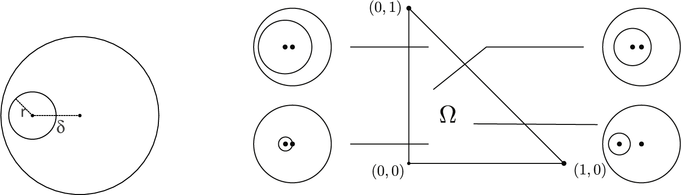
In this work, we study billiards in annular tables as introduced by Saitô et al in [Reference Saitô, Hirooka, Ford, Vivaldi and Walker24]. An annular table is a closed planar region
 $Q_{\delta ,r}\! \subset {\mathbb R}^2$
bounded by a unitary circle
 $\gamma $
centered at the origin, and an inner circle
 $\alpha $
of radius r centered at a point
 $p_{\delta }$
at a distance
 $\delta $
from the origin. We call the exterior unitary circle the exterior boundary and the inner circle is called the obstacle. The distance
 $\delta $
between the centers is called the eccentricity. The set of parameters is the triangular region
 $ \Omega =\{(\delta ,r): 0\leq \delta <1 \mbox { and } 0< {r + \delta } <1\}$
(see Figure 1). The corresponding two-parameter family of billiard maps is denoted by
 $T_{\delta ,r}$
. As the collisions with the inner circle carry the interesting part of the dynamics, it is meaningful to describe the dynamics through the first return to the obstacle map, denoted by
 $G_{\delta ,r}$
. Our results are stated for this first return map and, correspondingly, we refer in this introduction to the set of collisions with the obstacle as the phase space.
The annular table and the parameter space
 $\delta \times r$
.

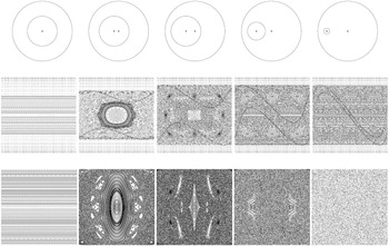
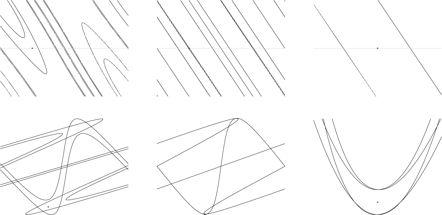
It is important to have in mind that the circular billiard alone, without the inner obstacle, is completely integrable. However, the dynamics purely generated by the inner circle is somehow equivalent to Sinai’s billiard which is ergodic. Billiards in annular tables may share the properties of these two classical examples and exhibit a combined mixed dynamics. In particular, it was observed that the annular billiard undergoes very interesting dynamical bifurcations as one varies the parameters. The dynamics ranges from integrability (when the circles are concentric) to chaotic (when the obstacle is small and close to the exterior boundary). Between these two extreme situations, the typical mixed Hamiltonian dynamics appears with elliptical islands surrounded by chaotic regions. The complexity of this dynamics, as observed numerically in [Reference Saitô, Hirooka, Ford, Vivaldi and Walker24], can be seen in Figure 2.
Change of the dynamics with the parameters as viewed from the collisions with the external boundary (
 $M_{\mathrm{out}}$
) and with the obstacle (
 $M_{\mathrm{inn}}$
).

We have here a scenario similar to other families of conservative systems as, for instance, the standard map [Reference Duarte17, Reference Gorodetski20]. Among billiards we mention, on one hand, the different types of stadiums [Reference Bálint, Halász, Hernández-Tahuilán and Sanders1, Reference Canale, Markarian, Oliffson Kamphorst and Pinto-de Carvalho10] and mushrooms [Reference Bunimovich8] and, on the other hand, the moon [Reference Correia and Zhang13] and lemon [Reference Bunimovich, Zhang and Zhang9] billiards.
More general systems of convex boundaries with inner scatters have been studied by several authors, among whom we cite Foltin, Chen, and Bolotin [Reference Bolotin6, Reference Chen11, Reference Foltin19]. Foltin [Reference Foltin19] showed that for a generic choice of convex external boundary, the system has positive topological entropy provided the obstacle’s radius is small enough. This result was also obtained by Chen in [Reference Chen11] using different techniques. In both works, the dynamics around a specific class of periodic trajectories colliding orthogonally with the obstacle (we will refer to these as normal periodic trajectories) is at the center of the proof. The result follows from the fact that under certain generic conditions, the dynamics in a neighborhood of such normal periodic orbits is conjugated to a shift. Bolotin [Reference Bolotin6] has proved that also under generic conditions on the external boundary and for small obstacles, the system presents hyperbolic sets around the normal periodic orbits. All these results were obtained by perturbation of the convex boundary and apply to generic situations. They do not apply to the annular billiard, as the circular shape of the exterior boundary is certainly not generic. Nevertheless, we use here some similar techniques and the role of normal trajectories is also central.
Billiards in annular tables, as they have both convex and concave components, are examples of the so-called focusing and dispersing dynamics. It is well known that the dynamical behavior of such systems depend on the balance of these two effects. In systems with convex components sufficiently far apart, hyperbolicity is generated through the defocusing mechanism [Reference Bunimovich7, Reference Donnay16]. This is not the situation for the annular billiard and the standard defocusing arguments do not apply, as well as for moon and lemon billiards [Reference Bunimovich, Zhang and Zhang9, Reference Correia and Zhang13]. These three models fall in a different category of systems, where hyperbolicity comes from other mechanisms. In this work, we show how to calibrate the distance between the centers and the radius of the inner circle to obtain hyperbolicity in large parts of the phase space of the annular billiard. As pointed out by previous results and numerical experiments, this hyperbolicity occurs for large eccentricity and small obstacle, that is,
 $\delta \approx 1$
and
 $r \approx 0$
.
Thus, if on one hand, hyperbolicity seems to come from the dispersive obstacle, on the other hand, the convexity of the outside boundary seems to be related to stability and Kolmogorov–Arnold–Moser phenomena. The existence of stable periodic orbits in the annular billiard, in particular, the one of period 2, was investigated by Saitô et al [Reference Saitô, Hirooka, Ford, Vivaldi and Walker24], while an extensive study of other periodic orbits was presented by Gouesbet et al [Reference Gouesbet, Meunier-Guttin-Cluzel and Gréhan21]. For small eccentricity, stable orbits of small period can be observed [Reference Batista3, Reference de Moraes Costa14]. The large island of a period-2 trajectory which exists for
 $r>\delta $
is clearly visible in Figure 2 as well as a period four and a period six. As one changes the parameters in the opposite direction by increasing the eccentricity (and decreasing the size of the obstacle), the islands become smaller and the orbits undergo transitions from elliptic to hyperbolic. In particular, Saitô et al point out that the system seems to become ergodic as
 $\delta \to 1$
and
 $r \to 0$
if one considers only the trajectories which collide with the obstacle. In this work, we focus on this last situation and look for hyperbolic behavior. More recently, Dettmann and Fain [Reference Dettmann and Fain15] exhibited families of stable normal periodic orbits in the annular billiard when the obstacle is small and near the boundary, concluding that the system cannot be ergodic for open sets of values of parameters close to this limit. The result is obtained through an explicit construction of suitable orbits and a direct computation of their nonlinear stability. The existence of elliptical island follows from Birkhoff’s normal form and Moser’s twist theorem. This is sometimes a tricky problem involving hard computations in very specific situations. Also for small obstacles and large eccentricity, we obtain elliptical islands associated to a bifurcation of homoclinic tangencies (Newhouse phenomenon). As far as we know, this is the first time that this mechanism is described explicitly in billiards.
The presence of these elliptical islands gives a negative answer to the question if, as in the case of stadium-like systems, there is a region in the parameter space where the annular billiard is fully chaotic (that is, has positive Lyapunov exponent in a region of full measure). It is natural to ask if there are any values of the parameters such that the chaotic region has positive measure. This is a challenging question, as well as the question of the size of the region occupied by islands. Another challenging question is the existence (or not) of other dynamical elements characteristic of conservative systems such as invariant rotational curves and Aubry–Mather sets.
The goal here is to present a global picture of the dynamics on annular billiards for large eccentricity and small obstacle considering hyperbolic and non-hyperbolic properties. The big picture we obtain is the following: for many values of parameters corresponding to a small eccentric obstacle, the system presents an ‘almost dense’ hyperbolic horseshoe, corroborating the numerical observation of ‘chaos’ in [Reference Saitô, Hirooka, Ford, Vivaldi and Walker24]. However, the constructed hyperbolic set has zero measure and, in many cases, coexists with an also ‘almost dense’ set of elliptical islands originated from the generic bifurcation of quadratic homoclinic tangencies (Newhouse phenomenon).
Obtaining results for the annular billiard is somehow simplified by the fact that it is generated by two simple dynamics where the calculations can be made explicitly. What makes the situation more delicate is that the system is singular due to the existence of trajectories that are tangent to the obstacle which implies a loss of regularity and of compacity. To overcome this difficulty, in §2, after writing down the billiard map explicitly, we describe the domain of the first return to the obstacle map
 $G_{\delta ,r}$
with special attention on the image and preimages of its boundary. Understanding the geometry of these singular curves as the parameters
 $(\delta ,r)$
converge to
 $(1,0)$
is crucial along this work.
The key point to obtain hyperbolicity is that through a careful analysis of the tangent map
 $DG_{\delta ,r}$
as
 $r \to 0$
, we can identify a strong expansion direction in a certain region of the phase space. This fact gives rise to the hyperbolicity since it allows construction of a cone field as described in §3. These cones are preserved along orbits staying in these regions, which motivates the search for periodic orbits. In particular, a family of normal periodic points is at the core of the construction of a hyperbolic set and in §4, we show the abundance of these points.
Our first result is the existence of hyperbolic sets which become ‘large’, in the sense that they converge to the entire phase space, as the obstacle decreases in size and approaches the external boundary.
Theorem 1. There is an open set of parameters
 $\Omega _0$
accumulating
 $(1,0)$
and a piecewise continuous family
 $\Omega _0 \ni (\delta ,r) \mapsto \Lambda _{\delta ,r}$
of horseshoes for the first return to the obstacle map
 $G_{\delta ,r}$
such that the maximum distance of any point of the phase space to
 $\Lambda _{\delta ,r}$
goes to zero as
 $(\delta ,r) \rightarrow (1,0)$
.
The proof of the above theorem is in §5. A compact invariant set in the region of hyperbolicity is constructed from the normal trajectories which, colliding orthogonally with the obstacle, originate periodic points of the first return map. Using the cones described in §3 in subsets around these periodic orbits, we construct hyperbolic invariant sets, the horseshoes mentioned in the statement of the theorem. As a part of this construction, we obtain a symbolic description of the dynamics in the hyperbolic set
 $\Lambda _{\delta ,r}$
. We show that the map
 $G_{\delta ,r}$
restricted to it is conjugated to a subshift with a number of symbols which grows to infinity as
 $(\delta ,r) \to (1,0)$
.
Analytically, a normal orbit corresponds to the intersection of two curves in the phase space, which is transverse in the hyperbolic region. Outside the hyperbolic region, there are tangent normal points which turn out to be closely related to non-hyperbolicity. In the last section, we show how tangent normal periodic points give rise to tangencies of invariant manifolds. We are able to show that for many parameters, quadratic homoclinic tangencies between manifolds of points in the set
 $\Lambda _{\delta ,r}$
appear.
Theorem 2. There is a set
 $\Omega ^{\prime }_0 \subset \Omega _0$
accumulating
 $(1,0)$
such that the maps
 $G_{\delta ,r}$
, for
 $(\delta ,r) \in \Omega _0'$
, present quadratic homoclinic tangencies unfolding generically with the parameter r.
Unlike the general setting of quadratic tangencies in dimension 2 between invariant one-dimensional foliations, where one has to deal with the delicate analysis of intersection of Cantor sets [Reference Palis and Takens23], here the reversibility of the system plays a major role. This follows from the fact that if a branch of a stable manifold intersects the symmetry curve, then we automatically obtain a homoclinic point of the basic set. Thus, quadratic tangency between a branch of a stable manifold with the symmetry curve implies quadratic homoclinic tangency.
As a consequence of the bifurcation of the homoclinic tangencies, the annular billiard presents the so-called conservative Newhouse phenomenon with the appearance of many elliptical islands. In fact, a detailed analysis of the bifurcation process enables one to use Duarte’s theorem [Reference Duarte18] to prove that for many values of the parameters, the annular billiard has elliptical islands scattered across the phase space. This is the content of our third theorem, also in §6. The last statement of the theorem strongly relies on our accurate description of the hyperbolic sets.
Theorem 3. There is a set
 $\Omega _0''$
accumulating
 $(1,0)$
such that if
 $(\delta ,r) \in \Omega _0''$
, then the map
 $G_{\delta ,r}$
has a set
 $\mathcal {E}_{\delta ,r}$
of generic elliptic periodic points. Moreover, the distance of any point of the phase space to
 $\mathcal {E}_{\delta ,r}$
tends to zero as
 $(\delta ,r) \rightarrow (1,0)$
.
In short, we were able to discriminate dynamical structures that appear in the phase space of the annular billiard (hyperbolic sets and elliptical islands) in the small and eccentric obstacle limit. However, we do not have an estimate of the measure of the chaotic region and, in fact, we do not even know if it is positive. Moreover, even if the elliptical islands clearly sum up to a positive measure region, we do not know its extension. The estimates of the size of a specific elliptical island are in general hard to produce, as they usually involve a thorough analysis of normal forms. Moreover, concerning the islands resulting from the Newhouse phenomenon in our case, we only know, as a general fact, that they exist and have long period (and so small islands).
As a conclusion, we mention that there are several interesting questions concerning annular billiards besides the (Lebesgue) measure of the chaotic region. For instance, it is natural to ask if the closure of the union of the hyperbolic set(s) we produce and the islands has full measure and, if not, what is its complement? Furthermore, one would like to have a more precise description of the bifurcation set, specially the parameter set corresponding to homoclinic or heteroclinic tangencies. There is also the question of the dynamics inside an elliptical island, from the point of view of Zehnder’s genericity or the existence of instability regions (in the sense of Birkhoff) containing a hyperbolic set inside an island. This problem is possibly related to the destruction of invariant curves for parameters near the concentric case (although this is a very degenerate situation) or to the transition of the stability of the orbits of period 2 (trajectories orthogonal both to the obstacle and to the external boundary) or higher. Finally, we point out that some of the results we obtained here are also true for generic external convex boundaries [Reference Batista4].
To summarize, the sketch of the paper is the following. In §2, we present the annular billiard and the first return to the obstacle maps as well as the domain, with special attention on the singularities. Section 3 contains the definition and properties of a cone field and §4 the description of normal periodic orbits. These are the ingredients to construct a hyperbolic set and prove Theorem 1 in §5. Finally, in §6, we show how homoclinic tangencies are produced (Theorem 2) and, as a consequence, we have the existence of elliptical islands (Theorem 3).
2 Preliminaries
The billiard problem originally consists of a description of the free motion of a point particle in a bounded region of the plane with elastic collisions at the boundary. Conservation of energy and linear momentum implies the reflection law at impact. As a conservative system with two degrees of freedom, each state is given by a point in the region and a unitary vector which accounts for the direction of motion. After some identifications, the time evolution is given by a three-dimensional flow [Reference Chernov and Markarian12, Reference Foltin19], which in our case is defined for all time. It is usual to study the billiard dynamics through a restriction to the Poincaré section taken at the boundary of the region. The billiard map is then defined by the first return to boundary and thus associates to each impact, the next one.
Given an annular region
 $Q_{\delta ,r}\! \subset {\mathbb R}^2$
, we assume that the normal vectors point inside it. The external circular boundary
 $\gamma $
is parameterized by its central angle
 $s \in \mathbb {S}^{1}$
and is oriented counterclockwise, while the inner circular obstacle
 $\alpha $
is parameterized by its central angle
 $\omega \in \mathbb {S}^1$
, and is oriented clockwise. Here, we consider
 ${\mathbb S^1} \sim (-\pi ,\pi ]$
. As usual, the billiard map is described by two variables: one for the position on the boundary (s or
 $\omega $
) and one for the direction of the trajectory, given by the oriented angle from the inward normal vector to the outgoing velocity (
 $\theta $
at the exterior boundary and
 $\beta $
at the obstacle). A collision with the external circle
 $\gamma $
is then represented by a point
 $(s,\theta )$
in the open cylinder
 $M_{\mathrm{out}}= \mathbb {S}^1\times (-{\pi }/{2},{\pi }/{2})$
and a collision with the obstacle
 $\alpha $
is represented by a point
 $(\omega , \beta )$
in the closed cylinder
 $M_{\mathrm{inn}}=\mathbb {S}^1\times [-{\pi }/{2},{\pi }/{2}]$
. The disconnected phase space of the billiard map
 $T=T_{\delta ,r}$
is the union
 $M=M_{\mathrm{out}} \cup M_{\mathrm{inn}}$
. We observe that the map may be extended by considering the boundary of
 $M_{\mathrm{out}}$
as fixed points. To lighten our notation, we will frequently omit the subscript
 $\delta ,r$
that indicates the dependence of the maps and sets on the parameters. We will also refer to the inner circle as the obstacle and to the external circle simply as the circle or the boundary.
So,
 $T: M \rightarrow M$
denotes the billiard map in the annular region in general. It is well defined and is invertible, as it is reversible with respect to the involution
 $R(a,b)= (a,-b)$
, i.e.
 $ T^{-1}=R \circ T \circ R$
. This reversibility implies that the phase space is symmetric with respect to the middle horizontal line. In particular, every orbit has its symmetrical which corresponds to the same trajectory traveled in the opposite direction.
As described below, T is defined by parts: it is a piecewise diffeomorphism with a singular set generated by the tangent collisions with the concave obstacle. Here, T is globally
 $C^0$
and piecewise
 $C^{\infty }$
.
To describe T, we must distinguish between three different situations: the collisions from the obstacle to the (external) circle, from the circle to the obstacle, and from the circle to the circle. Any trajectory from the obstacle will hit the circle in the sequence, which implies that
 $T(M_{\mathrm{inn}}) \subset M_{\mathrm{out}}$
and
 $T^{-1}(M_{\mathrm{inn}}) \subset M_{\mathrm{out}}$
. A trajectory leaving the circle will hit the obstacle if and only if
 $|\!\sin \theta + \delta \sin (\theta -s)| \le r$
. We introduce the sets
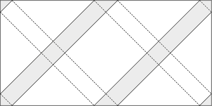
 $$ \begin{align} T(M_{\mathrm{inn}}) &= M_{\mathrm{inn}}^+=\{(s,\theta): |\!\sin \theta + \delta \sin (\theta+ s)| \leq r\}, \\ T^{-1}(M_{\mathrm{inn}}) &= M_{\mathrm{inn}}^-= \{(s,\theta): |\!\sin \theta + \delta \sin (\theta- s)| \leq r\} ,\nonumber \end{align} $$
which are topological cylinders in
 $M_{\mathrm{out}}$
(Figure 3).
 $M_{\mathrm{inn}}^+$
(gray) and
 $M^-_{\mathrm{inn}}$
(white) in the complement of the whispering gallery in
 $M_{\mathrm{out}}$
(scaled), for
 $r>\delta $
,
 $r<\delta $
,
 $r \ll \delta $
,
 $r \ll \delta \approx 1$
.

The restriction
 $T: M_{\mathrm{inn}}\rightarrow M_{\mathrm{inn}}^+$
(from the obstacle to the boundary) is implicitly given by
 $$ \begin{align} T(\omega,\beta)=(s,\theta) \mbox{ with} \begin{cases} \sin \theta +\delta \sin(\theta+s)=-r\sin\beta,&\\ \omega+\beta= -s-\theta, & \\ \mbox{and } |\!\sin\theta+\delta\sin(\theta+s)|\leq r. \end{cases} \end{align} $$
Considering the trajectories leaving the exterior boundary, the restriction
 $T: M_{\mathrm{inn}}^-\rightarrow M_{\mathrm{inn}}$
(from the boundary to the obstacle) is implicitly given by
 $$ \begin{align} T(s,\theta)=(\omega,\beta) \mbox{ with} \begin{cases} \sin \theta +\delta \sin(\theta-s)=-r\sin\beta,&\\ \omega-\beta= \theta-s ,& \\ \mbox{where } |\!\sin\theta+\delta\sin(\theta-s)|\leq r. \end{cases} \end{align} $$
In the particular case of a trajectory from the boundary to the boundary without colliding with the obstacle, the map
 $T:M_{\mathrm{out}}\setminus M_{\mathrm{inn}}^- \rightarrow M_{\mathrm{out}}$
is given by the circular billiard map (denoted by F)
 $$ \begin{align} T(s,\theta) = F(s,\theta)=(s + \pi -2\theta, \theta). \end{align} $$
The map from the exterior boundary is then clearly discontinuous on
 $T^{-1}(\partial M_{\mathrm{inn}})$
. The concavity of the obstacle implies the existence of unavoidable tangent collisions corresponding to
 $\partial M_{\mathrm{inn}} = \{ \beta = \pm \pi /2 \}$
. Moreover, the map T is not differentiable on
 $\partial M_{\mathrm{inn}}$
. The map T has then a singular set given by the curves
 $\partial M_{\mathrm{inn}} \cup T^{-1}(\partial M_{\mathrm{inn}})$
and the inverse
 $T^{-1}$
has a singular set
 $\partial M_{\mathrm{inn}} \cup T(\partial M_{\mathrm{inn}})$
. Out of the singular set, T is a
 $C^\infty $
diffeomorphism.
It is also well known that the billiard map is conservative and preserves the measure
 $\mu $
given in
 $M_{\mathrm{out}}$
by
 $d\mu = \cos \theta \,ds\, d\theta $
and in
 $M_{\mathrm{inn}}$
by
 $ d \mu = r\cos \beta d\omega d\beta $
. In the canonical variables (tangential momentum and arc length), the Lebesgue measure
 $dpds$
is preserved. This can also be directly checked from the expressions in equations (2.2), (2.3), and (2.4) above. The choice of the coordinate
 $\omega $
in
 $M_{\mathrm{inn}}$
instead of the usual arc length is particularly convenient as we want to use arguments with
 $r \to 0$
.
Trajectories leaving the exterior boundary in almost tangential directions will circulate around without hitting the obstacle. More precisely, if a trajectory leaves the exterior boundary with an angle
 $|\!\sin \theta |> \delta + r$
, it will follow the circular billiard motion forever with a circular caustic concentric to the boundary. The corresponding invariant region in
 $M_{\mathrm{out}}$
is a cylinder foliated by invariant rotational horizontal curves, clearly visible in Figure 2. This region is known as the whispering gallery and we denote it by
 $M_{w} \subset M_{\mathrm{out}}$
. In addition to the whispering gallery, there are other trajectories from the exterior boundary which do not hit the obstacle. They necessarily correspond to periodic orbits in
 $M^c_w \backslash (M^+_{\mathrm{inn}} \cup M^-_{\mathrm{inn}}) \subset M_{\mathrm{out}}$
as any non-periodic trajectory in the circular billiard would be dense on the caustic of radius
 $|\!\sin \theta | < r+ \delta $
and so cannot avoid the obstacle.
However, a trajectory leaving the obstacle and hitting the boundary with
 $|\!\sin \theta | < \delta + r$
will hit the obstacle again an infinite number of times. As for
 $|\!\sin \theta | = \delta +r$
, the only trajectories leaving the obstacle and not returning to it occur when the orbit of a tangent point
 $(\omega ,\beta ) = (\pi , \pm {\pi }/{2})$
of
 $M_{\mathrm{inn}}$
is not periodic (the trajectory corresponds to the circular billiard caustic of radius
 $\delta + r$
). So, with a possible exception of two points, every point
 $(\omega ,\beta ) \in M_{\mathrm{inn}}$
has a finite return time to
 $M_{\mathrm{inn}}$
:
 $$ \begin{align*}\nu (\omega,\beta)= \mathrm{min}\{j \geq 1: T^j(z) \in M_{\mathrm{inn}}\}.\end{align*} $$
This will allow us to define the first return to the obstacle map
 $$ \begin{align*}G = M_{\mathrm{inn}} \rightarrow M_{\mathrm{inn}}, \,\,\,\, G(\omega,\beta)= T^{\nu(\omega,\beta)} (\omega,\beta)= T\circ F^{\nu(\omega,\beta) - 2} \circ T (\omega,\beta).\end{align*} $$
So, a trajectory leaving the obstacle from
 $(\omega _0,\beta _0)$
will return to it at
 $(\omega _1,\beta _1) = G (\omega _0,\beta _0) $
after
 $m = \nu (\omega _0,\beta _0)-2$
collisions with the external boundary at points
 $(s_0,\theta _0) = T(\omega _0,\beta _0), \ldots , (s_m,\theta _0) = F^m (s_0,\theta _0)$
with
 $(\omega _1,\beta _1) = T (s_m,\theta _0)$
.
From the properties of the billiard map, G is a piecewise
 $C^\infty $
diffeomorphism. We denote its set of singularities by
 $\mathcal {S}^- = \partial M_{\mathrm{inn}} \cup G^{-1}(\partial M_{\mathrm{inn}})$
. The singular set of
 $G^{-1}$
is denoted by
 $\mathcal {S}^+ = \partial M_{\mathrm{inn}} \cup G(\partial M_{\mathrm{inn}})$
.
The annular billiard has two period-two trajectories, bouncing between the obstacle and the exterior boundary with orthogonal collisions. They correspond to the fixed points of the first return map G:
 $(0,0)$
and
 $(\pi , 0)$
. The second is always hyperbolic, while the first one is hyperbolic if
 $r<\delta $
and elliptic (in fact, Moser stable) if
 $r>\delta $
[Reference Batista2, Reference Batista3, Reference de Moraes Costa14, Reference Saitô, Hirooka, Ford, Vivaldi and Walker24]. The annular billiard has also many other periodic normal trajectories, as the orbits presented in §4, which play a very important role in the dynamics and in our analysis, as in [Reference Chen11, Reference Foltin19]. The stability of some of these orbits was established in [Reference Dettmann and Fain15]. It is clear that the stability of periodic orbits and the dynamics depend on the parameters. In particular, numerical experiments seem to indicate that, in addition to the period-2 orbit, the other short period elliptical orbits also loose stability as r decreases. This is one reason why, to investigate the chaotic behavior of the annular billiard, we focus on the dynamics for small
 $r<\delta $
. More precisely, we will present results on the two-parameter family of maps
 $G_{\delta ,r}$
, describing some aspects of the dynamics as
 $(\delta ,r) \rightarrow (1,0)$
.
In our strategy, the parameter dependence of some relevant subsets of the phase space is very important. The sets
 $M^+_{\mathrm{inn}}$
and
 $M^-_{\mathrm{inn}}$
are contained in the cylinder
 $ M^c_w {\kern-1pt}={\kern-1pt} |\!\sin \theta | {\kern-1pt}\le{\kern-1pt} r {\kern-1pt}+{\kern-1pt} \delta $
, the complement of the whispering gallery in
 $M_{\mathrm{out}}$
. The boundaries of these cylindrical sets, as defined in equation (2.1), are given by the curves
 $$ \begin{align*} \partial M^{\pm}_{\mathrm{inn}} = |\!\sin \theta + \delta \sin (\theta \pm s) | = r, \end{align*} $$
which have a single point of tangency with the top and the bottom of
 $M^c_w$
. For fixed
 $\delta $
, the whispering gallery grows when the obstacle becomes smaller and so these sets become thinner as r goes to 0, as we will present below (see Figure 3).
If we denote the horizontal line corresponding to orbits leaving the obstacle in the normal direction by
 $$ \begin{align} L^0 = \{(\omega, \beta) \mid \beta = 0 \}\subset M_{\mathrm{inn}}, \end{align} $$
its image and preimage in
 $M_{\mathrm{out}}$
are defined by
 $$ \begin{align} L_{\delta}^+ =T(L^0) &= \{(s,\theta): \sin \theta + \delta \sin (\theta+ s)= 0\} ,\\ L_{\delta}^-= T^{-1}(L^0) &=\{(s,\theta): \sin \theta + \delta \sin (\theta- s)=0\}. \nonumber \end{align} $$
We notice that these sets depend only on
 $\delta $
, the eccentricity parameter.
It follows that the boundaries
 $\partial M_{\mathrm{inn}}^+$
and
 $\partial M_{\mathrm{inn}}^-$
converge as r goes to 0 respectively to the curves
 $ L_{\delta }^+$
and
 $L^-_{\delta }$
. Therefore, as
 $r \to 0$
, the subsets
 $M_{\mathrm{inn}}^\pm $
become narrow cylindrical strips that also converge to the curve
 $L_{\delta }^\pm $
. This contraction has deep consequences on the dynamical behavior. We also point out that the curves
 $ L_{\delta }^+$
and
 $L^-_{\delta }$
are graphs of analytic functions of
 $\theta $
converging uniformly in
 $(-\pi , \pi )$
, as
 $\delta \to 1$
to the lines
 $2 \theta \pm s = 0$
. As for any
 $\delta $
,
 $s=\pm \pi $
implies
 $\theta = 0$
, the limit is strongly discontinuous.
Another relevant preliminary observation is that for
 $\delta> r$
, the domains
 $M^+_{\mathrm{inn}}$
and
 $M^-_{\mathrm{inn}}$
do not contain any horizontal line
 $\theta = \mathrm{constant}$
. Moreover, in this case, the intersection
 $M^+_{\mathrm{inn}} \cap M^-_{\mathrm{inn}}$
as two distinct connected components, each one containing one period-2 orbit, correspond to the two fixed points of the first return to the obstacle map:
 $(0,0)$
and
 $(\pi ,0) \in M_{\mathrm{inn}}$
.
We note again that, to make the notation lighter and the reading easier, we will drop the subscripts
 $\delta ,r$
of maps and sets in our proofs and computations whenever the parameters are fixed and the dependence on them is clear.
3 Finding regions of hyperbolicity: cone fields
In this section, we will show that the annular billiard presents hyperbolicity for a wide choice of parameters. This hyperbolicity follows from the existence of a cone field, which, in some region of the collision with the obstacle set
 $M_{\mathrm{inn}}$
, is strictly preserved by the first return to the obstacle map G. As vectors in the cone are uniformly expanded, any invariant compact set will be uniformly hyperbolic.
Defining horizontal/vertical cone fields
 $z \mapsto C^{\pm }(z)$
for
 $z=(\omega ,\beta ) \in \mathrm{int} \, M_{\mathrm{inn}}$
by
 $$ \begin{align} C^+(z) &:= \{u=(u_1,u_2) \in {\cal T}_{z}M: u_2.u_1 \geq 0\}, \\ C^-(z) &:= \{u=(u_1,u_2) \in {\cal T}_{z}M: u_2.u_1 \leq 0\}, \nonumber \end{align} $$
we have the following theorem.
Theorem 3.1. There is a subset
 $\Omega _* \subset \Omega $
of parameters such that for each
 $(r,\delta ) \in \Omega _{*}$
, there are subsets
 $H_{\delta ,r}^{\pm } \subset M_{\mathrm{inn}}$
with
 $H_{\delta ,r}^+=G_{\delta ,r}(H_{\delta ,r}^-)$
, where:
-
(i) the map
 $ G_{\delta ,r}: H_{\delta ,r}^- \rightarrow H_{\delta ,r}^+$
(respectively
$G_{\delta ,r}^{-1}: H_{\delta ,r}^+ \rightarrow H_{\delta ,r}^-$
) strictly preserves the cone field
$C^+$
(respectively
$C^-$
);
-
(ii) for points in
$H_{\delta ,r}^{-}$
(respectively
$H_{\delta ,r}^{+} $
) (3.2)with
$$ \begin{align} \|D G_{\delta,r} \| \mbox{ (respectively }\|D G_{\delta,r}^{-1}\|\mbox{)} \geq \rho \end{align} $$
$\rho \rightarrow \infty $
as
$r \rightarrow 0$
.


As a consequence, we obtain the following corollary.
Corollary 3.2. If
 $(\delta ,r) \in \Omega _*$
and
 $\Lambda \subset H_{\delta ,r}^-$
is a compact invariant set for
 $G_{\delta ,r}$
then
 $\Lambda $
is a uniformly hyperbolic set for
 $G_{\delta ,r}$
.
As usual, we will drop the subscript
 $\delta ,r$
in maps and sets.
Let us consider a trajectory leaving the obstacle with
 $(\omega _0,\beta _0) \in M_{\mathrm{inn}} \backslash {\mathcal S}^-$
and returning to it with
 $(\omega _1,\beta _1)=G(\omega _0,\beta _0)$
, after
 $m+1$
impacts with the exterior border
 $\gamma $
given by
 $\{(s_0,\theta ),\ldots ,(s_{m},\theta )\}$
. A straightforward computation from equations (2.3), (2.2), and (2.4) leads to the following expression of the derivative of the map:
 $$ \begin{align} DG{(\omega_0,\beta_0)}= \left( \begin{array}{cc} a_{11} & a_{12}\\ a_{21}&a_{22} \end{array}\right)= a_{21} \left( \begin{array}{cc} 1 & 1\\ 1&1 \end{array}\right) + \left( \begin{array}{cc} \widetilde{a}_{11} & \widetilde{a}_{12}\\ 0 & \widetilde{a}_{22} \end{array}\right)\!\kern-1pt, \end{align} $$
where
 $$ \begin{align} a_{21} = -\frac{\cos \theta}{r \cos \beta_1} \bigg( \frac{\delta \cos \varphi_0}{\cos \theta} + \frac{\delta \cos \varphi_1}{\cos \theta} + 2(m+1) \frac{\delta \cos \varphi_0}{\cos \theta} \, \frac{\delta \cos \varphi_1}{\cos \theta} \bigg) \end{align} $$
and
 $$ \begin{align} \widetilde{a}_{11} & = \displaystyle 1 + {2(m+1)}\frac{\delta\cos\varphi_0}{\cos\theta}, \\ \widetilde{a}_{22} & = \displaystyle \frac{\cos\beta_0}{\cos\beta_1} \bigg( 1 + {2(m+1)}\frac{\delta\cos\varphi_1}{\cos\theta}\bigg), \nonumber\\ \widetilde{a}_{12} & = \displaystyle 1+ \frac{\cos\beta_0}{\cos\beta_1} + 2(m+1) \bigg(\frac{\delta\cos\varphi_0}{\cos\theta} + \frac{\cos\beta_0}{\cos\beta_1}\frac{\delta \cos\varphi_1}{\cos\theta}- r\frac{\cos\beta_0}{\cos\theta} \bigg)\nonumber\\ & = \widetilde{a}_{11} + \widetilde{a}_{22} - 2 r (m+1) \frac{\cos\beta_0}{\cos\beta_1}. \nonumber \end{align} $$
Here,
 $\varphi _0 = s_0 + \theta = -\omega _0 -\beta _0$
and
 $\varphi _1= s_m - \theta = -\omega _1 + \beta _1$
represent the angle between the outgoing trajectory leaving the obstacle (respectively incoming back) and the horizontal direction. It is worthwhile to note that
 $\det DG = \cos \beta _0 /\cos \beta _1$
.
The key observation is that as r approaches zero, the first matrix in the sum dictates the behavior of the tangent map as long as
 $a_{21} \ne 0$
. However, it is easy to check that
 $a_{21}$
is negative at
 $(0,0)$
and positive at
 $(\pi ,0)$
, corresponding to the 2-periodic trajectories. However, it is clear that
 $a_{21}$
vanishes if the trajectory paths between the obstacle and the boundary are vertical, as
 $\varphi _0 = \varphi _1 = \pm \pi /2$
. These observations indicate that there is no hope to bound
 $a_{21}$
away from zero globally on
 $M_{\mathrm{inn}}$
. Our strategy then is to find a subset of parameters
 $\Omega _*$
and a subset of phase space
 ${H}^-_{\delta ,r}$
where all the entries of the matrix
 $DG$
are non-zero and have the same sign. This will imply the preservation of the cone
 $C^+$
for G and, by reversibility, also implies the preservation of the cone
 $C^-$
by
 $G^{-1}$
[Reference Wojtkowski27, Reference Wojtkowski28].
Lemma 3.3. Let
 $ \zeta = {\delta \cos \varphi }/{\cos \theta } $
. If
 $\delta ^2> \tfrac 12 $
and
 $ r< \tfrac 14(\delta -\delta ^2)$
, then for any
 $\varphi \in [0,2\pi ]$
,
 $\theta \in [-\pi /2,\pi /2]$
such that
 $|\!\sin \theta + \delta \sin \varphi | \le r $
and
 $|\!\sin \theta | \le \delta ^2$
, we have
 $$ \begin{align*} \zeta_{\mathrm{min}} = \frac{\delta}{2}\sqrt{\frac{3}{1+\delta^2}} < |\zeta| < \sqrt{\delta}= \zeta_{\mathrm{max}}. \end{align*} $$
Moreover,
 $\zeta _{\mathrm {min}}>1/2$
and
 $\zeta _{\mathrm {max}} < 1$
.
Proof. If we use the coordinates
 $x = -\delta \sin \varphi $
and
 $y = \sin \theta $
, we have that
 $\zeta ^2 = ({\delta ^2 {\kern-1.2pt}-{\kern-1.2pt} x^2})/({1{\kern-1.2pt}-{\kern-1.2pt}y^2})$
should be bounded on the compact parallelogram
 $\{(x,y){\kern-1.2pt}:{\kern-1.2pt} |y{\kern-1.2pt}-{\kern-1.2pt}x|\leq r \mathrm {and} \, \, |y|\leq \delta ^2\}$
. As
 $\nabla \zeta ^2 = {2}/({1-y^2}) (-x,\zeta ^2 y)$
, the origin is the only critical point inside the domain. It is a saddle with
 $\zeta ^2(0,0)=\delta ^2$
, and so minimum and maximum should be on the boundary. Because of the symmetry of the function
 $\zeta ^2$
, we can restrict our search for the maximum and minimum values to the region bounded by the lines
 $y = x+ r$
,
 $y=x-r$
,
 $y=\delta ^2$
, and the axes
 $x=0$
,
 $y= 0$
.
The level curves of
 $\zeta ^2 = k^2$
are the hyperbolas
 $ k^2 - \delta ^2 = k^2 y^2 - x^2 $
and so, corresponding to
 $\zeta ^2 = \delta ^2$
, we have the asymptotes
 $x^2 = \delta ^2 y^2$
. The hyperbolas with vertices on the y axis have
 $\zeta ^2> \delta ^2$
and those with vertices on the x axis correspond to
 $\zeta ^2 < \delta ^2$
. This implies that the maximum value of
 $\zeta ^2$
occurs on the segment of the line
 $y=x+r$
between the y axis and the asymptote
 $x=\delta y$
, that is, between the points
 $(0,r)$
and
 $(\delta r/(1-\delta ), r/(1-\delta ))$
. Moreover, at the maximum point
 $(x^*,y^*)$
, we have that
 $\nabla \zeta ^2. (1,1)$
= 0 and so the maximum value
 $\zeta ^2(x^*,y^*) = x^*/y^*$
. As
 $x^* = y^* - r$
, it follows that
 $\zeta ^2 (x^*,y^*) = 1 - r/y^*$
and since
 $r<y^*<r/(1-\delta )$
, we have that
 $$ \begin{align*}\zeta^2(x^*,y^*)< \delta < 1.\end{align*} $$
Since the slope of the components of the boundary is 1 or 0, it is clear that no hyperbola with
 $\zeta ^2 < \delta ^2$
can have a tangency with them and so the minimum value must occur at a vertex. Comparing the values, and using that
 $r< 1/4 (\delta -\delta ^2)$
, it is easy to check that the minimum value is
 $$ \begin{align*} \frac{\delta^2-(\delta^2+r)^2}{{1-\delta^4}} = \frac{((\delta-\delta^2) - r)(\delta+\delta^2+r)}{(1+\delta^2)(1-\delta^2)}> \frac{3}{4} \, \frac{\delta^2}{1+\delta^2} > \frac{1}{4}.\\[-42pt] \end{align*} $$
Following Lemma 3.3 above, we define the horizontal strip
 $H_{\delta } = \{(s,\theta )$
such that
 $|\!\sin \theta | < \delta ^2 \} \subset M_{\mathrm{out}}$
and the subsets of
 $M_{\mathrm{inn}}$
:
 $$ \begin{align} H_{\delta,r}^- = T^{-1} (H_{\delta}), \quad H_{\delta,r}^+ = T(H_{\delta}), \quad\mbox{and}\quad \bar{H}_{\delta,r}= H_{\delta,r}^+ \cap H_{\delta,r}^-. \end{align} $$
Its easy to check that
 $G(H_{\delta ,r}^-)= H^+_{\delta ,r}$
and
 $R(H^-_{\delta ,r})= H^+_{\delta ,r}$
, and from equations (2.3) and (2.2), we have
 $$ \begin{align} H^{\pm}_{\delta,r}= \{(\omega,\beta): |\delta\sin(\omega\mp \beta)+r\sin\beta|<\delta^2\}. \end{align} $$
As noticed at the end of §2, if
 $r<\delta $
, the intersection of any horizontal strip in
 $M_{\mathrm{out}}$
with either
 $M^+_{\mathrm{inn}}$
or
 $M^-_{\mathrm{inn}}$
has two distinct connected components. So,
 $H^\pm _{\delta ,r} \subset M_{\mathrm{inn}}$
also have two connected components, one containing the point
 $(0,0)$
and the other the point
 $(\pi ,0)$
. These components are bounded by the four curves with endpoints in
 $\partial M_{\mathrm{inn}}$
given by
 $ |\delta \sin (\omega \mp \beta )+r\sin \beta |=\delta ^2$
. Each of the components of
 $M_{\mathrm{inn}} \backslash H^\pm _{\delta ,r}$
contains one of the points
 $(-{\pi }/{2},0 )$
or
 $({\pi }/{2},0 )$
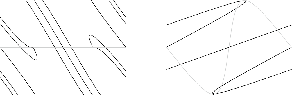
(Figure 4).
 $H^+_{\delta ,r}\! \subset M_{\mathrm{inn}}$
for
 $r>\delta $
,
 $r<\delta $
,
 $r \ll \delta $
,
 $r \ll \delta \approx 1$
.

Fixing
 $\delta $
and taking
 $r\rightarrow 0$
, the curves in
 $\partial H_{\delta ,r}^- \backslash \partial M_{\mathrm{inn}}$
converge to the straight lines given by
 $|\!\sin (\omega +\beta )|=\delta $
. Thus, as
 $(\delta ,r) \rightarrow (1,0)$
, the components of
 $M_{\mathrm{inn}} \backslash H_{\delta ,r}^-$
shrink to the decreasing lines
 $\omega +\beta = \pm {\pi }/{2}$
and hence the set
 $H^-_{\delta ,r}$
converges, in Hausdorff sense, to
 $M_{\mathrm{inn}}$
. Similarly, as
 $(\delta ,r) \rightarrow (1,0)$
, the components of
 $M_{\mathrm{inn}} \backslash H^+_{\delta ,r}$
shrink to the lines
 $\omega -\beta = \pm {\pi }/{2}$
, and
 $H^-_{\delta ,r}$
converges to
 $M_{\mathrm{inn}}$
.
Lemma 3.4. For
 $\delta ^2> \tfrac 12$
and
 $r< \tfrac 14(\delta -\delta ^2)$
, if
 $(\omega _0,\beta _0) \in H^-_{\delta ,r}$
, then
 $|a_{21}| \geq {4A}/{\sqrt {r}}$
, where A is a constant depending only on
 $\delta $
.
Proof. Using the notation of Lemma 3.3, we can write
 $$ \begin{align*} a_{21} = - \frac{\cos \theta}{r \cos \beta_1} (\zeta_0 + \zeta_1+ 2(m+1) \zeta_0 \zeta_1). \end{align*} $$
As
 $(\omega _0,\beta _0) \in \bar {H}$
and we have
 $r<\tfrac 14(\delta -\delta ^2)$
,
 $$ \begin{align*}\cos^2 \theta> 1 - \delta^4 = (1+\delta^2)(1+\delta)(1-\delta) \ge \delta(1-\delta) > 4r. \end{align*} $$
For any
 $m\geq 0$
, we consider
 $$ \begin{align*}g_{m} (x,y) = 2(m+1) x y + x + y\end{align*} $$
in the region
 $D=\{(x,y): \zeta _{\mathrm {min}} \leq |x|, |y| \leq \zeta _{\mathrm {max}} \}$
, which corresponds to four equal squares in the plane, and we want to estimate its minimum value. Here,
 $g_m$
has a saddle point at
 $( {-1}/{2(m+1)} , {-1}/{2(m+1)} )$
with
 $g_m = -1/2(m+1)$
. The level curves are hyperbolas with asymptotes through the saddle point parallel to the
 $x,y$
axes. There are two distinct level curves with
 $g_m=0$
, one through
 $(0,0)$
and the other through
 $( {-1}/({m+1}) , {-1}/({m+1}) )$
. These level curves are outside the four squares as
 $\zeta _{\mathrm {min}}>1/2$
and
 $\zeta _{\mathrm {max}} <1$
, and so the minimum value should be on one of the corners. It is easy to check that in fact the minimum occurs at the vertex closest to the point
 $( {-1}/({m+1}) , {-1}/({m+1}) )$
. For
 $m=0$
, it is the point
 $(-\zeta _{\mathrm {min}},-\zeta _{\mathrm {min}})$
, while for
 $m\ge 1$
, it is
 $(-\zeta _{\mathrm {max}},-\zeta _{\mathrm {max}})$
. It follows that
 $$ \begin{align*} | \zeta_0 + \zeta_1 + 2(m+1) \zeta_0 \zeta_1 | \ge \begin{cases} 2 (\zeta_{\mathrm{max}} - \zeta_{\mathrm{max}}^2) & \mbox{ if }m=0, \\ 2 ((m+1) \zeta_{\mathrm{min}}^2 - \zeta_{\mathrm{min}}) \ & \mbox{ if }m \ge 1. \end{cases} \end{align*} $$
So we have
 $|g_0| \ge 2(\sqrt {\delta } - \delta )$
and for
 $m\ge 1$
,
 $|g_m| \ge |g_1| \ge 2 ( {6\delta ^2}/{2(1+\delta ^2)}- {\delta \sqrt {3}}/{2\sqrt {1+\delta ^2}}) $
. If we denote
 $$ \begin{align} A= \min \bigg\{(\sqrt{\delta}-\delta), \bigg( \frac{6\delta^2}{2(1+\delta^2)}- \frac{\delta\sqrt{3}}{2\sqrt{1+\delta^2}}\bigg)\bigg\}, \end{align} $$
the lower bound on
 $|a_{21}|$
follows. In fact, we have
 $g_0 \ge 2A$
and for
 $m \ge 0$
,
 $$ \begin{align*} |g_{m}| \geq (m+1) A.\\[-36pt] \end{align*} $$
Lemma 3.5. For
 $\delta ^2> \tfrac 12$
and
 $r< \tfrac 14(\delta -\delta ^2)$
, if
 $(\omega _0,\beta _0) \in H^-_{\delta ,r}$
, then
 $$ \begin{align*} \bigg | \frac{\widetilde{a}_{11}}{a_{21}} \bigg | \le A_{11} \sqrt{r}, \quad \bigg | \frac{\widetilde{a}_{22}}{a_{21}} \bigg | \le A_{22} \sqrt{r}, \quad \bigg | \frac{\widetilde{a}_{12}}{a_{21}} \bigg |\le A_{12} \sqrt{r}, \end{align*} $$
where the constants
 $A_{11}, A_{22}$
, and
 $A_{12}$
depend only on
 $\delta $
.
Proof. Following the notation and definitions in the proof of Lemma 3.4 above, we have
 $$ \begin{align*} \bigg|\frac{\widetilde{a}_{11}}{a_{21}}\bigg| & = \bigg|\frac{r\cos\beta_1}{ \cos \theta}\bigg| |f_{m}(\zeta_0,\zeta_1)|,\\ \bigg|\frac{\widetilde{a}_{22}}{a_{21}}\bigg| & = \bigg|\frac{r\cos\beta_0}{\cos \theta}\bigg| |f_{m}(\zeta_1,\zeta_0)|, \\ \bigg|\frac{\widetilde{a}_{12}}{a_{21}}\bigg| &\leq \bigg|\frac{\widetilde{a}_{11}}{a_{21}}\bigg|+ \bigg|\frac{\widetilde{a}_{22}}{a_{21}}\bigg| + \bigg| \frac{r\cos\beta_0}{\cos\theta}\bigg| \bigg| \frac{r\cos\beta_1}{\cos\theta}\bigg| \bigg| \frac{1}{g_{m}(\zeta_0,\zeta_1)}\bigg|, \end{align*} $$
where
 $$ \begin{align*} f_{m}(\zeta_0,\zeta_1)= \frac{1+2(m+1) \zeta_0}{g_{m}(\zeta_0,\zeta_1). } \end{align*} $$
If
 $ \zeta _{\mathrm {min}} \le |\zeta _i| \le \zeta _{\mathrm {max}}$
, we have
 $$ \begin{align*}|f_m (\zeta_0,\zeta_1)| \leq \frac{4(m+1)\sqrt{\delta}}{(m+1)A}= \frac{4\sqrt{\delta}}{A}\end{align*} $$
and as
 $1/ \cos \theta < \sqrt {r}/2$
, it follows that
 $$ \begin{align*} \bigg|\frac{\widetilde{a}_{11}}{a_{21}}\bigg| \leq \frac{2\sqrt{\delta}}{A} \sqrt{r},\quad \bigg|\frac{\widetilde{a}_{22}}{a_{21}}\bigg| \leq \frac{2\sqrt{\delta}}{A}\sqrt{r},\quad \bigg|\frac{\widetilde{a}_{12}}{a_{21}}\bigg| \leq \frac{4\sqrt{\delta}+1/4}{A}\sqrt{r}.\\[-42pt] \end{align*} $$
Proof of Theorem 3.1
With the constant A defined by equation (3.8), we consider the continuous function:
 $$ \begin{align*}r(\delta) < \min \bigg \{ \frac{1}{4}(\delta-\delta^2), \frac{A^2}{(1/4+ 4\sqrt{\delta})^2}\bigg\}\end{align*} $$
and define the set of parameters:
 $$ \begin{align} \Omega_{*}= \big\{(\delta,r):\delta^2> \tfrac{1}{2} \text{ and } 0<r<r(\delta)\big\}, \end{align} $$
which is has no empty interior and accumulates
 $(1,0)$
as
 $A\to 0$
when
 $\delta \to 1$
.
It is then clear that if
 $(\delta ,r) \in \Omega _{*}$
and
 $(\omega ,\beta ) \in H^-_{\delta ,r}$
, the matrix
 $DG(\omega ,\beta )$
as given in equation (3.3) has either positive or negative entries and so the cone field
 $C^+$
is strictly preserved. Moreover, taking
 $u=1/\sqrt {2}(1,1) \in C^+$
, we have
 $$ \begin{align*} DG(\omega,\beta) u = a_{21} \left[ \left( \begin{array}{@{}c@{}} \sqrt{2}\\ \sqrt{2} \end{array} \right) + \frac{1}{\sqrt{2} \, a_{21}} \left( \begin{array}{@{}c@{}} a_{11} + a_{12} \\ a_{22} \end{array} \right) \right] \end{align*} $$
with, from Lemma 3.5,
 $ e = ({\sqrt {(a_{11}+a_{12})^2 + a_{22}^2}}/ { \sqrt {2} |a_{21}| }) < K \sqrt {r} $
for some constant K depending only on
 $\delta $
.
We have then
 $$ \begin{align} \| DG(\omega,\beta)\| \ge \| DG(\omega, \beta) \, u \| \ge |a_{21}| ( 2- e)> \rho, \end{align} $$
where
 $\rho $
is a constant depending only on
 $\delta $
, which can be chosen using the bound on
 $a_{21}$
from Lemma 3.4. Moreover,
 $\rho \to \infty $
as
 $ r\to 0$
.
By reversibility,
 $G^{-1}: H_{\delta ,r}^+ \backslash {\mathcal S}^+ \rightarrow H_{\delta ,r}^- \backslash {\mathcal S}^-$
preserves the cones
 $C^-$
, expanding vectors by the rate
 $\rho $
.
A closer look at the tangent map
 $DG$
as given by equation (3.3) shows that as
 $r\to 0$
, it strongly contracts vectors to the diagonal
 $(1,1)$
direction, while the inverse
 $DG^{-1}$
contracts to
 $(-1,1)$
. We can use this fact to obtain more precise estimates on the expansivity and control on the hyperbolicity. To do so, we introduce the notion of stable and unstable curves, which play a fundamental role in our geometric arguments to exhibit both hyperbolic and non-hyperbolic behavior in the annular billiard, as studied in §§5 and 6.
Definition 3.6. For
 $(\delta ,r) \in \Omega _*$
, let
 $$ \begin{align*} c_1 =\min_{(\omega,\, \beta) \in {H}^{-}_{\delta,r} } \frac{a_{21}(\omega, \beta)}{a_{11}(\omega, \beta)} \quad\text{and}\quad c_2 = \max_{(\omega,\, \beta) \in {H}^{-}_{\delta,r}} \frac{a_{22}(\omega, \beta)}{a_{12}(\omega, \beta)}, \end{align*} $$
and note that
 $c_1, c_2 \to 1$
as
 $r\to 0$
. A
 ${\mathcal C}^1$
-curve
 $\ell (t) = (\omega (t),\beta (t))$
is called unstable if
 $\ell (t) \subset {H}^{-}_{\delta ,r}$
and
 $c_1 \leq {\beta '(t)}/{\omega '(t)} \leq c_2$
, and it is called stable if
 $\ell (t) \subset {H}^+_{\delta ,r}$
and
 $-c_2 \leq {\beta '(t)}/{\omega '(t)} \leq -c_1$
. If
 $\beta '(t)=0$
, the curve is horizontal.
We summarize in the following propositions some properties of stable and unstable curves which can be easily derived from the arguments leading to Theorem 3.1.
Proposition 3.7. Let
 $\ell $
be a
 ${\mathcal C}^1$
-curve and
 $|\ell |$
denote its length. Then, for
 $(\delta ,r) \in \Omega _*$
, the following properties hold.
-
(1) If
$\ell $
is stable (unstable), then it is the graph
$\omega =f(\beta )$
of a
$1/c_1$
-Lipschitz monotone function f. Moreover, for
$r \approx 0$
, a stable (unstable) curve is
$\mathcal {C}^1$
close to a straight segment of slope
$-1 (1)$
. -
(2) If
$\ell \subset H^-_{\delta ,r}$
is either an unstable or a horizontal curve, then
$G_{\delta ,r}(\ell )$
is unstable and
$|G_{\delta ,r}(\ell )| \geq \rho |L|$
. -
(3) If
$\ell \subset H^+_{\delta ,r}$
is either a stable or a horizontal curve, then
$G_{\delta ,r}^{-1}(\ell )$
is stable and
$|G_{\delta ,r}^{-1}(\ell )| \geq \rho |\ell |$
.


As defined by equation (3.10), the expansion rate
 $\rho $
depends only on
 $\delta $
and goes to
 $\infty $
as
 $r\to 0$
.
We also have the following description of the set of the singularities of
 $G: M_{\mathrm{inn}} \rightarrow M_{\mathrm{inn}}$
, given by
 ${\mathcal S}_{\mathrm{inn}}^-= \partial M_{\mathrm{inn}} \cup G^{-1}(\partial M_{\mathrm{inn}})$
and its inverse.
Proposition 3.8. For
 $(\delta ,r) \in \Omega _{*}$
, the singular set of the restriction
 $G_{\delta ,r}: H_{\delta ,r}^- \rightarrow H_{\delta ,r}^+$
consists of segments of curves either stable or horizontal. Analogously, the singular set of the restriction
 $G_{\delta ,r}^{-1}: H_{\delta ,r}^+ \rightarrow H_{\delta ,r}^-$
consists of segments of curves either unstable or horizontal.
Proof. From equations (2.2), (2.3), or also from general results about the set of singularities of billiards [Reference Chernov and Markarian12], the singular set consists of an union of compact arcs of
 ${\mathcal C}^\infty $
curves with no other intersection than its endpoints. As the curves in
 $\partial M_{\mathrm{inn}}$
are horizontal, to characterize the singular set of G, we only need to analyze curves in
 $\partial G^{-1}(M_{\mathrm{inn}} )$
. Let us consider a smooth component of
 $(\mathcal {S}_{\mathrm{inn}}^-\cap H_{\delta ,r}^-)\cap \partial G^{-1}(M_{\mathrm{inn}} ) $
. Any such curve is the pre-image
 $G^{-1}(\ell )$
of some (horizontal) curve
 $\ell \subset \partial M_{\mathrm{inn}}$
. Taking a sequence
 $\{ \ell _{n} \}$
of horizontal curves in
 $H_{\delta ,r}^+ \backslash \mathcal {S}_{\mathrm{inn}}^+$
converging, in
 $\mathcal {C}^1$
topology, to the curve
 $\ell $
as
 $n \rightarrow \infty $
, from Proposition 3.7,
 $\{G^{-1}(\ell _{n})\}$
is a sequence of stable curves approaching
 $G^{-1}(\ell )$
as
 $n \rightarrow \infty $
. This implies that
 $G^{-1}(\ell )$
is a stable curve.
4 Normal periodic points
Our strategy to obtain both hyperbolicity and non-hyperbolicity is based on the study of the behavior of the first return to the obstacle map G in the neighborhood of some particular periodic orbits known as normal orbits [Reference Foltin19]. A normal periodic trajectory leaves the obstacle
 $\alpha $
in the normal direction and, after hitting the exterior circle
 $\gamma $
at
 $m+1 $
points (
 $m\ge 1$
), collides with the obstacle again in the normal direction and, therefore, the same path is traversed with reversed orientation giving rise to an orbit of period 2 for G (or period
 $2(m+2)$
for T), as shown in Figure 5. The two 2-periodic trajectories, one from
 $\omega =\pi $
and the other from
 $\omega = 0$
, which exist for any values of the parameter, are also normal orbits with
 $m=0$
. Both correspond to fixed points of G. There are also normal periodic orbits with more intermediate hits on the obstacle between the two normal hits, as well as non-periodic trajectories with only one normal hit on the obstacle. However, we will not consider these two last kinds of normal trajectories and, unless specified, we will use the term normal orbits (or trajectories) only to refer to the two 2-periodic trajectories and to trajectories with exactly two (normal) impacts with the obstacle.
Normal trajectories.

The annular billiard has many normal orbits and, in fact, their number increases as r decreases. Examples of normal orbits may be constructed in the annular billiard from trajectories leaving the obstacle in the normal direction and colliding with the external boundary with a rational angle
 $\theta = ({p}/{q})\pi $
. This situation corresponds to a piece of a trajectory in the circular billiard passing twice through the center of the obstacle. Clearly, this construction produces a normal periodic trajectory in the annular billiard for every r small enough (Figure 5). It is also clear that the path, and so the period of a normal orbit, for a given
 $\delta $
, remains unchanged as r decreases. As
 $r\to 0$
, each rational
 $\theta $
will define a normal orbit, implying that the number of normal (periodic) orbits tends to infinity in this limit. The unlimited increase of the number of normal orbits is fundamental in our arguments.
In an abuse of language, for a given
 $\delta $
, we will call a point
 $(\omega , 0)$
simply a normal point if it corresponds to a normal orbit (with two normal hits on the obstacle) for r small enough, even though strictly speaking, any point
 $(\omega , 0)$
corresponds to a trajectory leaving the obstacle in the normal direction.
In general, as the curve
 $L^0 \subset M_{\mathrm{inn}}$
defined by equation (2.5) denotes the set of orthogonal collisions with the obstacle, normal points
 $(\omega ,\beta =0)$
correspond to the intersection
 $L^0 \cap G^{-1} (L^0) \subset M_{\mathrm{inn}}$
. It follows that
 $(s,\theta ) = T(\omega ,0) \in L_{\delta }^+ \cap F^{-m}(L_{\delta }^-) \in M_{\mathrm{out}}$
and so normal points correspond to the solutions of the system
 $$ \begin{align} L^+_{\delta}:& \sin\theta - \delta \sin \omega =0, \nonumber\\ F^{-m}(L_{\delta}^-):&\sin\theta - \delta \sin( \omega - (m+1) (\pi -2\theta))=0. \end{align} $$
It is worthwhile to notice that normal orbits are symmetric, in the sense that if
 $(s,\theta )$
belongs to the orbit, so does the point
 $(s,-\theta )$
.
A normal trajectory of period
 $2 (m+2)$
is specified by
 $$ \begin{align*} \{ (\omega_0, \beta = 0), (s_0,\theta_0), \ldots, (s_m,\theta_m), (\omega_1, 0) \} \mbox{ with }s_k = s_0 + k (\pi - 2 \theta_0) \mbox{ and }\theta_k = \theta_0, \end{align*} $$
with
 $s_0 = -\theta _0 -\omega _0$
,
 $\omega _1 = \theta _0 - s_m$
, and where
 $\omega _0$
and
 $\theta _0$
must satisfy the system in equation (4.1) above. In particular, for any fixed
 $m \ge 1$
, this system has a solution with
 $\theta $
rational, that is, a rational multiple of
 $\pi $
. However, a solution of the above system will be a normal orbit in the annular billiard if
 $|\!\sin \theta _k + \delta \sin (\theta _k - s_k) |> r $
for
 $ 0 \le k < m$
, which clearly is verified for any r small enough. This shows that for any
 $\delta $
fixed, the number of normal periodic orbits goes to infinity as r decreases to zero.
Definition 4.1. A point
 $(\omega ,0) \in L^0 \cap G^{-1}(L^0)$
is a transverse (respectively tangent) normal point if the intersection is transverse (respectively tangent).
Whether a normal point
 $(\omega ,0)$
is transverse or not depends on the intersection
 $T(\omega , 0) \in L_\delta ^+ \cap F^{-m}(L_{\delta }^-)$
. From equation (4.1), we have that a tangency occurs if and only if
 $$ \begin{align} &\cos \theta (\cos \omega- \cos (\omega - (m+1)(\pi - 2 \theta)) = 2 (m+1) \delta \cos \omega \cos (\omega - (m+1)(\pi - 2 \theta)) \nonumber \\ &\qquad\qquad\qquad\qquad\quad\mbox{with } \sin \omega = \sin (\omega - (m+1)(\pi - 2 \theta)). \end{align} $$
This implies that tangencies are given by
 $$ \begin{align} \cos \omega = 0 \quad \mbox{or} \quad \frac{\delta \cos \omega}{\cos \theta} = \frac{-1}{m+1}. \end{align} $$
It follows from Lemma 3.3 that, for
 $(\delta ,r) \in \Omega _{*}$
, all normal points in
 $H^-_{\delta ,r}$
are transverse. Outside
 $H^-_{\delta ,r} \cup H^{+}_{\delta ,r}$
, we will consider only tangent normal points given by
 $\cos \omega = 0$
, as in Figure 5. As already observed in §3, this last condition implies that
 $a_{21} = 0$
in the tangent map
 $DG$
and so these trajectories represent an obstruction to hyperbolicity as obtained there. In fact, we shall see that transverse normal points give rise to hyperbolicity, while tangent normal points are related to non-hyperbolic dynamics.
We emphasize that trajectories of normal points depend only on
 $\delta $
(continuously) and do not depend on r, since this variable does not intervene in the system in equation (4.1) or equations (4.2) and (4.3). This is an important remark, as it allows us to use the limit
 $r \to 0$
.
5 Hyperbolic sets around transverse normal points
In this section, we will prove Theorem 1 by exhibiting a set of parameters
 $\Omega _0$
, where each first return to the obstacle map
 $G_{\delta ,r}$
has a horseshoe
 $\Lambda _{\delta ,r}$
. The point
 $(\delta =1,r=0)$
is an accumulation point of the set
 $\Omega _0$
and the family of horseshoes
 $\Lambda _{\delta ,r}$
converges to the entire phase space as
 $(\delta ,r) \rightarrow (1,0)$
. The construction of the horseshoes follows standard arguments as in [Reference Wiggins26] and uses, in addition to the preservation of cones, the geometric properties of the maps in the neighborhood of transverse normal points, which we describe below.
Following the construction in §4, given
 $\delta \in [1/\sqrt {2}, 1)$
, we can choose
 $\omega _i $
, such that
 $(\omega _i,0)$
is a transverse normal point for every r sufficiently small. We denote by
 $S_i$
the closure of the connected component of
 $M_{\mathrm{inn}} \backslash \mathcal {S}_{\mathrm{inn}}^-$
containing
 $(\omega _i,0)$
, so all the points in
 $\mathrm{ int } (S_i)$
have the same returning time
 $\nu = \nu (\omega _i,0)$
. The normal trajectory of
 $(\omega _i,0)$
is
 $2\nu $
periodic and has only two collisions with the obstacle. Since by definition, normal trajectories have no tangential collisions with the obstacle, the billiard map T, and so the first return map G, is a
 ${\mathcal C}^{\infty }$
diffeomorphism in
 $\mathrm {int} (S_i)$
. Again, we often omit the dependence on
 $\delta $
and r of the maps and sets; however, we stress that most of the properties of normal transverse periodic orbits depend only on
 $\delta $
and are actually continuous on this parameter. A key point in our geometric construction of horseshoes is that, for small r,
 $S_i$
and
 $U_i=G(S_i)$
are essentially parallelograms with two sides in the distinct components of
 $\partial M_{\mathrm{inn}}$
. This geometric concept will be important in our arguments.
Definition 5.1. A compact connected set
 $ \mathbf {S} \subset M_{\mathrm{inn}}$
is essentially a parallelogram if its boundary is the union of four distinct curves that are
 $\mathcal {C}^1$
close to the sides of a parallelogram.
Definition 5.2. A compact connected set
 $ \mathbf {S} \subset M_{\mathrm{inn}}$
bounded by two disjoint stable (unstable) curves connecting the two opposite components of
 $\partial M_{\mathrm{inn}}$
, will be called a stable (unstable) strip.
The expression connecting
 $\partial M_{\mathrm{inn}}$
will be always mean connecting the two different components of
 $\partial M_{\mathrm{inn}}$
.
Lemma 5.3. For each fixed eccentricity
 $\delta \in [1/\sqrt {2}, 1)$
, and any normal point
 $(\omega _i,0)$
, with
 $|\!\sin \omega _i| < \delta $
, there is
 $r_i$
such that for all
 $r \leq r_i$
, the following properties hold.
-
(1)
$S_{i} \ni (\omega _i,0)$
is a stable strip bounded by two stable curves in
$G^{-1}(\partial M_{\mathrm{inn}})$
connecting the two distinct components
$\partial M_{\mathrm{inn}}$
and converging in the
${\mathcal C}^1$
topology to the decreasing straight line
$J_i^-= \{(\omega ,\beta ): \omega + \beta = \omega _i\}$
as
$r\rightarrow 0$
. -
(2)
$U_{i} \ni G(\omega _i,0) = (\hat \omega _i,0)$
is an unstable strip bounded by two unstable curves in
$G(\partial M_{\mathrm{inn}})$
connecting
$\partial M_{\mathrm{inn}}$
and converging in the
${\mathcal C}^1$
topology to the increasing straight line
$J_i^+= \{(\omega ,\beta ): \omega - \beta = \hat \omega _i\}$
as
$r\rightarrow 0$
.


Proof. By reversibility, it is enough to prove property (1). The first return to the obstacle time of
 $(\omega _i,0)$
is
 $\nu (\omega _i,0) = m_i+2$
for some integer
 $m_i \ge 0$
. So, the first return map restriction
 $G: S_i \rightarrow U_i$
decomposes as
 $G=T \circ F^{m_i} \circ T$
and by definition,
 $S_i$
is the connected component containing
 $(\omega _i,0)$
of the set
 $ M_{\mathrm{inn}} \cap G^{-1}(M_{\mathrm{inn}}) \backslash (T^{-2}(M_{\mathrm{inn}}) \cup \cdots \cup T^{-m_i-1}(M_{\mathrm{inn}})). $
To describe
 $S_i$
, we consider its image
 $T(S_i)$
which is a subset of
 $M_{\mathrm{inn}}^+ \cap F^{-m_i}(M_{\mathrm{inn}}^-)$
. If
 $V_i$
denotes the connected component of
 $M_{\mathrm{inn}}^+ \cap F^{-m_i}(M_{\mathrm{inn}}^-)$
containing
 $T(\omega _i,0)$
, it is clear that
 $T(S_i) \subset V_i$
and we have
 $$ \begin{align} T(S_i) = V_i \backslash (F^{-1}(M_{\mathrm{inn}}^-) \cup \ldots F^{-m_i+1}(M_{\mathrm{inn}}^-)) \subset M_{\mathrm{inn}}^+ \cap F^{-m_i}(M_{\mathrm{inn}}^-) \subset M_{\mathrm{out}}. \end{align} $$
As observed at the end of §2,
 $\partial M_{\mathrm{inn}}^{\pm } \underset {r \to 0}{\longrightarrow } L_{\delta }^{\pm }$
, so for
 $j= 0,\ldots ,m_i$
, we have
 $$ \begin{align} & F^{j} (\partial M_{\mathrm{inn}}^+) \underset{r \to 0}{\longrightarrow} F^{j}( L_{\delta}^+), \ F^{-j} (\partial M_{\mathrm{inn}}^-) \underset{r \to 0}{\longrightarrow} F^{-j}( L_{\delta}^-) \ \ \mbox{ in }C^\infty \mbox{ topology}, \\ & F^{\pm j} (M_{\mathrm{inn}}^\pm) \underset{r \to 0}{\longrightarrow} F^{\pm j}( L_{\delta}^\pm) \ \ \mbox{ in the Hausdorff set distance}. \nonumber \end{align} $$
The set H, defined in §3, is the horizontal strip
 $|\!\sin \theta | < \delta ^2$
, so the choice
 $|\!\sin \omega _i| $
means that
 $(\omega _i,0) \in H^{-}$
for any r and so it is a transversal normal point. It follows that the intersection
 $L^+_{\delta } \cap F^{-m_i}(L^-_{\delta })$
at
 $T(\omega _i,0)$
is also transversal. By definition,
 $V_i \subset M_{\mathrm{inn}}^+ \cap F^{-m_i}(M_{\mathrm{inn}}^-)$
, so this transversality and equation (5.2) imply that
 $$ \begin{align} F^{j} (V_i) \underset{r \to 0}{\longrightarrow} T^{j+1}(\omega_i,0) \quad\mbox{for}\ j=0,\ldots,m_i. \end{align} $$
However, as the first returning time is
 $m_i+2$
,
 $T^{{m_i}+1}(\omega _i,0) \in M_{\mathrm{inn}}^-$
, but
 $T^j(\omega _i, 0) \notin M_{\mathrm{inn}}^-$
for
 $j= 1, \ldots ,m_i$
. From equations (5.1) and (5.3), we can choose
 $r_i$
small enough that if
 $r \leq r_i$
, we have
 $F^j(V_i) \cap M_{\mathrm{inn}}^-= \emptyset $
for
 $j= 1, \ldots , m_i$
, implying that, in fact,
 $T(S_i)= V_i$
.
Furthermore, the convergence of
 $T(S_i)$
to
 $T(\omega _i,0)$
in equation (5.3) and the transversality of the intersection between
 $L_\delta ^+$
and
 $ F^{-m_i}(L_{\delta }^-) $
at this point, together with the convergence of
 $\partial M_{\mathrm{inn}}^+$
to
 $L_{\delta }^+$
and of
 $F^{-m_i}(M_{\mathrm{inn}}^-)$
to
 $F^{-m_i}(L_{\delta }^-) $
in equation (5.2), imply that for r small enough,
 $T(S_i)$
is essentially a parallelogram bounded by two curves in
 $\partial M_{\mathrm{inn}}^+$
and two curves in
 $F^{-m_i}(\partial M_{\mathrm{inn}}^-)$
. Hence,
 $S_i \subset M_{\mathrm{inn}}$
is a strip bounded by two curves in
 $T^{-1} \circ F^{-m_i}(\partial M_{\mathrm{inn}}^-) \subset G^{-1}(\partial M_{\mathrm{inn}})$
connecting
 $\partial M_{\mathrm{inn}}$
.
Moreover, we have that
 $T(\omega _i,0) = (s,\theta )$
with
 $|\!\sin \theta | < \delta ^2$
, which means that
 $T(\omega _i,0) \in H$
and clearly we can set
 $r_i$
such that
 $T(S_i)\subset H = T(H^-)$
implying that
 $S_i \subset H^-$
. Thus, the two curves connecting
 $\partial M_{\mathrm{inn}} \subset \partial S_i $
are stable, since they belong to the singular set
 $G^{-1}(\partial M_{\mathrm{inn}}) \cap H^{-}$
of G, as discussed in Proposition 3.8. This proves that
 $S_i$
is a stable strip.
To prove that
 $\partial S_i \to J^-_i$
, we refer to Proposition 3.7. The two opposite stable curves of
 $\partial S_i \subset S_i \cap G^{-1}(\partial M_{\mathrm{inn}})$
converge, in the
 ${\mathcal C}^1$
topology, to straight lines of slope
 $-1$
as
 $r\to 0$
. Now, consider a horizontal segment
 $\ell _\beta $
connecting these two curves. Its image
 $G(\ell _{\beta }) \subset U_i$
connects the components of
 $\partial M_{\mathrm{inn}}$
and
 $|G(\ell _{\beta })|> \rho |\ell _{\beta }|$
. However, as
 $G(\ell _{\beta })$
is a Lipschitz curve with a constant close to one connecting the boundaries, its length is less than some constant close to
 $\sqrt {2}$
and so for any
 $\beta $
,
 $|\ell _{\beta }| \lesssim \!{\sqrt {2}}/{\rho }$
. It follows that
 $|\ell _{\beta }| \to 0 $
uniformly as
 ${r \to 0}$
, implying that
 $S_i \rightarrow J_{i}^{-} $
as
 $ r \rightarrow 0$
.
The construction of the horseshoes for G is based on sets of transverse normal points
 $X_{\delta }$
which we describe bellow.
From the results of §4, for any arbitrary
 $\delta \in [1/\sqrt {2}, 1)$
, there is a dense set of points in
 $H^-_{\delta ,r} \cap L^0 = \{ (\omega ,0): |\!\sin \omega | < \delta \}$
that will give rise to transverse normal orbits as
 $r \rightarrow 0$
. In this dense set of transverse normal points, we can choose a set with
 $n_{\delta }$
points such that the
 ${\mathcal S}^1$
-distance between any two adjacent points is less than
 $d_{\delta } < \pi - 2 \arcsin \delta $
:
 $$ \begin{align} X_{\delta}= \{ (\omega_1,0), (\omega_2,0), \ldots (\omega_{n_{\delta}},0) \} \subset H^-_{\delta,r}. \end{align} $$
We observe that
 $ \pi - 2 \arcsin {\delta }$
is the length of each of the two disjoint components of the complement
 $L^0 - {H^-_{\delta ,r}}$
which are located around
 $(\omega = \pm \pi /2,0)$
. By including images, we can assume that
 $X_{\delta }$
is invariant under G. With this choice, the invariant set
 $X_{\delta }$
becomes dense in
 $L^0$
as
 $\delta \to 1$
and obviously
 $n_{\delta } = \# (X_{\delta }) \to \infty $
. It is important to notice that the set
 $X_{\delta }$
is robust on
 $\delta $
and does not depend on r as long it is sufficiently small. In particular,
 $H^-_{\delta ,r} \cap L^0$
does not depend on r.
Lemma 5.4. For each fixed
 $\delta \in [1/ \sqrt {2},1)$
, there is
 $r_{\delta }$
such that for any
 $r \in (0, r_{\delta }]$
, the map
 $G_{\delta ,r} $
has a locally maximal transitive hyperbolic set
 $\Lambda _{\delta ,r}$
such that the following properties hold.
-
(1) The restriction
$G_{\delta ,r}: \Lambda _{\delta ,r} \rightarrow \Lambda _{\delta ,r}$
is conjugated to a subshift in the space of sequences of
$n_{\delta }$
symbols. Moreover,
$n_{\delta } \to \infty $
as
$\delta \to 1$
. -
(2) The set
$\Lambda _{\delta ,r}$
is
$d_{\delta }$
-dense in
$M_{\mathrm{inn}}$
with
$d_{\delta } \rightarrow 0$
as
$\delta \rightarrow 1$
. -
(3) For any pair
$r' \ne r$
in
$(0,r_{\delta }]$
, the set
$\Lambda _{\delta ,r'}$
is the hyperbolic continuation of the set
$\Lambda _{\delta ,r}$
.


Proof. Given two distinct normal points
 $(\omega _i,0)$
and
 $(\omega _j,0)$
in
 $X_{\delta }$
, let
 $(\hat \omega _i, 0)=G(\omega _i,0) \in X_{\delta }$
. We will investigate the intersection
 $U_{i} \cap S_{j}$
, where
 $U_i \ni (\hat \omega _i,0) $
and
 $S_j \ni (\omega _j,0)$
. It follows from Lemma 5.3 that for small r, this intersection is related to the intersection of the lines
 $J_i^+ \ni (\hat \omega _i,0) $
and
 $J_j^- \ni (\omega _j,0)$
. It is obvious that
 $J_i^+\cap J_j^-$
consists of a single point in the interior of
 $M_{\mathrm{inn}}$
, unless
 $\hat \omega _i = \omega _j + \pi $
, in which case it consists of two points in the distinct components of
 $\partial M_{\mathrm{inn}}$
. As a consequence, if
 $ \hat \omega _i - \omega _j \neq \pi $
, for r small enough,
 $U_i \cap S_j$
is essentially a parallelogram bounded by two unstable curves in
 $\partial U_{i}$
and two stable curves in
 $\partial S_{j}$
.
In what follows, we consider
 $ 0< r_{\delta } < \min _{i = 1 \ldots n_{\delta }} r_i$
, where
 $r_i$
is given by Lemma 5.3. Clearly, we can also assume that
 $r_{\delta }$
is small enough so that
 $U_i$
effectively crosses
 $S_{j}$
whenever
 $ \hat \omega _i - \omega _j \neq \pi $
. It is also clear that by at least three points in the set
 $X_{\delta }$
, we will always have such crossings.
Given the set
 $X_{\delta }$
of
 $n_{\delta }$
transverse normal points, let us consider
 $ \Sigma =\{1,\ldots ,n_{\delta }\}^{\mathbb {Z}}$
, the space of sequences
 $a=\{a_i\} _{i \in \mathbb {Z}}$
of
 $n_{\delta }$
symbols, and the shift map
 $\sigma $
on it. We define
 $\widetilde {\Sigma } \subset \Sigma $
as the
 $\sigma $
-invariant subset of sequences such that for any
 $i \in \mathbb {Z}$
,
 $U_{a_i}=G(S_{a_{i}})$
crosses
 $S_{a_{i+1}}$
. Now, given a sequence
 $a = \{a_i\}_{i \in \mathbb {Z}} \in \widetilde {\Sigma }$
, we define the sets
 $$ \begin{align} S_{a}^n= \bigcap_{j=0}^nG^{-j}(S_{a_{j}}) \quad\mbox{and}\quad U_{a}^n= \bigcap_{j=0}^n G^{j}(U_{a_{\text{-}{(j+1)}}})\quad \mbox{for }n \geq 0. \end{align} $$
So,
 $S_{a}^{n+1} \subset S_{a}^n \ldots \subset S_a^0 = S_{a_0}$
and
 $U_{a}^{n+1} \subset U_{a}^n \ldots \subset U_a^0 = U_{a_{\text {-1}}}$
.
We will show that each
 $S_{a}^n$
is a stable strip bounded by stable curves in
 $G^{-(n+1)}(\partial M_{\mathrm{inn}})$
connecting
 $\partial M_{\mathrm{inn}}$
and similarly that each
 $U_{a}^n$
is an unstable strip bounded by unstable curves in
 $G^{(n+1)}(\partial M_{\mathrm{inn}})$
also connecting
 $\partial M_{\mathrm{inn}}$
. This is obviously true for
 $S^0_a = S_{a_0}$
and
 $U^0_a = U_{a_{\text {-1}}}$
by Lemma 5.3. Moreover, we note that by definition,
 $S^0_a$
crosses
 $U^0_a$
and so, when all the strips are stable or unstable, the intersections
 $S^{n}_a$
and
 $U^{n}_a$
also cross.
We have that
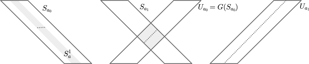
 $$ \begin{align} S_{a}^1= S_{a_0} \cap G^{-1}(S_{a_1}) = G^{-1}(G(S_{a_0}) \cap S_{a_1}) = G^{-1}(U_{a_0} \cap S_{a_1}). \end{align} $$
As
 $U_{a_0}$
is a strip bounded by two unstable curves in
 $G(\partial M_{\mathrm{inn}})$
and
 $S_{a_{1}}$
is a strip bounded by two stable curves in
 $G^{-1}(\partial M_{\mathrm{inn}})$
,
 $U_{a_0} \cap S_{a_{1}}$
is essentially a parallelogram bounded by two curves in
 $\partial U_{a_0}\cap G(\partial M_{\mathrm{inn}})$
and two curves in
 $\partial S_{a_1} \cap G^{-1}(\partial M_{\mathrm{inn}})$
. Its image under
 $G^{-1}$
is also essentially a parallelogram, bounded by two curves in distinct components of
 $\partial M_{\mathrm{inn}}$
and two stable curves in
 $G^{-2}(\partial M_{\mathrm{inn}})$
. Hence,
 $S_{a}^1$
is a stable strip in
 $S^0_{a} = S_{a_0}$
bounded by two opposite curves in
 $G^{-2}(\partial M_{\mathrm{inn}})$
. A similar argument shows that
 $U_{a}^1$
is an unstable strip in
 $U^0_{a} = U_{a_{\text {-1}}}$
bounded by two opposite curves in
 $G^{2}(\partial M_{\mathrm{inn}})$
(see Figure 6).
Construction of the sets
 $S_n$
.

The same construction can be applied to
 $S^n_a$
for
 $n>1$
, and also for
 $U^n_a$
. For instance,
 $$ \begin{align*}S^2_a= S_{a_0} \cap G^{-1}(S_{a_1}) \cap G^{-2}( S_{a_2}) = S^1_a \cap G^{-2} (S_{a_2}) = G^{-2}(G^2( S^1_a) \cap S_{a_2}). \end{align*} $$
By equation (5.6), we have
 $G^2(S_a^1)=G (U_{a_0} \cap S_{a_{1}}) $
. As
 $S_a^1$
has two boundaries in
 $G^{-2}(\partial M_{\mathrm{inn}})$
,
 $G^2(S_a^1)$
is a strip and, as the two other boundaries of
 $S_a^1$
are in
 $\partial M_{\mathrm{inn}}$
, their image under
 $G^{2}$
are unstable curves. So,
 $G^2(S_a^1)$
is an unstable strip in
 $G(S_{a_1}) =U_{a_1}$
and it must cross
 $S_{a_2}$
implying that the intersection
 $G^2(S_a^1) \cap S_{a_2}$
is also essentially a parallelogram with two boundaries in
 $G^2(\partial M_{\mathrm{inn}})$
and two in
 $G^{-1}(\partial M_{\mathrm{inn}})$
. It follows that
 $S_{a}^2 \subset S_{a}^1$
is a strip bounded by two stable curves in
 $G^{-3}(\partial M_{\mathrm{inn}})$
.
By induction, we assume that
 $S_{a}^{n-1}$
is a (stable) strip bounded by stable curves in
 $G^{-n}(\partial M_{\mathrm{inn}})$
. The definition in equation (5.5) can be written as
 $$ \begin{align*} S^{n}_a &= S_{a_0} \cap G^{-1}(S_{a_1}) \ldots \cap G^{-(n-2)}(S_{a_{n-2}}) \cap G^{-(n-1)}(S_{a_{n\text{-1}}}) \cap G^{-n}(S_{a_n}) \\ &= S^{n-1}_a \cap G^{-n}(S_{a_n} ) = G^{-n} (G^{n}(S^{n-1}_a) \cap S_{a_n} ). \end{align*} $$
The induction hypothesis implies that
 ${G^n}(S^{n-1}_a)$
is a strip bounded by two unstable curves in
 $G^n(\partial M_{\mathrm{inn}})$
connecting
 $\partial M_\alpha $
. As by definition,
 $S^{n-1}_a \subset G^{n-1}(S_{a_{n\text {-1}}})$
, we have that
 $G^n(S^{n-1}_a) \subset G(S_{a_{n\text {-1}}}) = U_{a_{n\text {-1}}}$
. It follows that
 $G^{n}(S^{n-1}_a) \cap S_{a_n} $
is essentially a parallelogram with two boundaries in
 $G^{n}(\partial M_{\mathrm{inn}})$
and two in
 $G^{-1}(\partial M_{\mathrm{inn}})$
, and so taking its image under
 $G^{-n}$
, we obtain that
 $S^{n-1}_a \cap G^{-n}(S_{a_n}) = S^{n}_a$
is a stable strip with boundaries in
 $G^{-(n+1)} \partial M_{\mathrm{inn}}$
.
Let us consider
 $S^n_a$
and a horizontal segment
 $\ell _{\beta }$
connecting the two opposite stable curves of
 $\partial S^n_a \subset G^{-(n+1)}(\partial M_{\mathrm{inn}})$
. Using an argument similar to the one at the end of the proof of Lemma 5.3, we have that the horizontal width of the strip
 $S^n_a$
is bounded by
 $|\ell _{\beta }| \lesssim {\sqrt {2}}/{\rho ^n} \to 0 $
as
 $n \to \infty $
. This convergence together with the properties of stable curves already stated imply that for any
 $a \in \tilde \Sigma $
,
 $S^{\infty }_a = {\bigcap _{n=0}^{\infty }} S^n_a$
is a decreasing
 $1/c_1$
-Lipschitz curve connecting
 $\partial M_{\mathrm{inn}}$
. From reversibility,
 $U_{a}^\infty $
is an increasing
 $1/c_1$
-Lipschitz curve connecting
 $\partial M_{\mathrm{inn}}$
. Hence, each
 $a \in \widetilde {\Sigma }$
corresponds to a unique point
 $S_a^\infty \cap U_a^\infty $
in
 $M_{\mathrm{inn}}$
and we can define a map
 $h: \widetilde {\Sigma } \rightarrow M_{\mathrm{inn}}$
given by
 $h(a)= S_{a}^\infty \cap U_{a}^\infty $
. Standard arguments [Reference Wiggins26] show that h is a homeomorphism onto its image.
To obtain the hyperbolic set, we define
 $\Lambda _{\delta ,r}=h(\tilde \Sigma )$
, which is a compact G-invariant set in
 $H_{\delta ,r}^-$
. The preservation of cones in
 $H_{\delta ,r}^-$
(Corollary 3.2) implies that
 $\Lambda _{\delta ,r}$
is a hyperbolic set for G. Moreover, the definition of h implies that G restricted to
 $\Lambda _{\delta ,r}$
is conjugated to the shift map
 $\sigma : \tilde \Sigma \rightarrow \tilde \Sigma $
.
For small r, the sets
 $S_i$
and
 $U_i$
are respectively close to the lines
 $J^-_i$
and
 $J^+_i$
. The points
 $J^-_i \pitchfork J^+_i = (\omega _i,0) \in X_{\delta }$
are
 $d_{\delta }$
-dense in
 $L^0$
and so we have a square lattice of lines
 $J^-_i$
and
 $J^+_k$
with
 $i, \,k=1\ldots n_{\delta }$
, whose nodes
 $J^-_i \pitchfork J^+_k$
are
 ${d_{\delta }}/{\sqrt {2}}$
-dense in
 $M_{\mathrm{inn}}$
. By definition, the points in
 $\Lambda _{\delta ,r}$
are close to the nodes in the interior of
 $M_{\mathrm{inn}}$
and therefore we can set
 $r_{\delta }$
such that the hyperbolic set itself is
 $d_{\delta }$
-dense in
 $M_{\mathrm{inn}}$
. It is clear from the construction that for each fixed
 $\delta $
and each
 $r \in (0,r_{\delta }] $
,
 $\Lambda _{\delta ,r}$
is a locally maximal transitive hyperbolic set. This implies that it has a continuation in r, which in turn is locally hyperbolic. More precisely, there is an open set
 $V \ni r$
such that for any
 $G_{\delta ,r'}$
with
 $r' \in V$
, the hyperbolic set
 $\Lambda _{\delta ,r'}$
is the continuation of
 $\Lambda _{\delta ,r}$
. As the argument holds for any r, we can take
 $ V = (0,r_{\delta }]$
. This proves item (3).
Lemma 5.5. For any
 $\delta \in [1/\sqrt {2},1)$
, there is a set of parameters
 $R_{\delta }=(\delta -\epsilon _{\delta },\delta + \epsilon _{\delta }) \times (0,r_{\delta }] \subset \Omega _*$
such that for any
 $(\delta ,r) \in R_{\delta }$
, the map
 $G_{\delta ,r}$
has a locally maximal transitive hyperbolic set
 $\Lambda _{\delta ,r}$
. Moreover, if
 $(\delta ',r')$
and
 $(\delta '', r'')$
are in
 $R_{\delta }$
, the set
 $\Lambda _{\delta '',r''}$
is the continuation of
 $\Lambda _{\delta ',r'}$
.
Proof. Given
 $\delta $
, the continuity and the transversality imply that if
 $\tilde \delta \approx \delta $
, for each
 $(\omega _i,0) \in X_{\delta }$
, we can find
 $\tilde \omega _i \approx \omega _i $
(called the continuation of
 $\omega _i$
) such that
 $(\tilde \omega _i, 0 )$
is also a transverse normal point of
 $G_{\tilde \delta , r}$
. In fact, there is
 $\epsilon _{\delta }$
and we can adjust
 $r_{\delta }$
such that if
 $|\widetilde {\delta }-\delta | {<} \epsilon _{\delta }$
, then the set
 $X_{\tilde \delta }$
obtained by continuation of
 $X_\delta $
contains also
 $n_{\delta }$
points which are normal transverse for any
 $0 < r\leq r_{\delta }$
. If necessary, we can take smaller
 $r_{\delta }$
and
 $\epsilon _{\delta }$
to ensure that
 $R_{\delta } = (\delta -\epsilon _{\delta },\delta + \epsilon _{\delta }) \times (0,r_{\delta }] \subset \Omega _*$
(as given by equation (3.9)).
Applying Lemma 5.4, we construct a locally maximal hyperbolic set
 $\Lambda _{\bar \delta ,r}$
for any
 $r \leq r_{\delta }$
. It is obvious that if
 $\delta '$
and
 $\delta ''$
are close, the square lattices obtained from
 $X_{\delta '}$
and
 $X_{\delta ''}$
, as in Lemma 5.4, are close for small values of r and so are the hyperbolic sets
 $\Lambda _{\delta ',r}$
and
 $\Lambda _{\delta '',r}$
. It follows from the continuity on
 $\delta $
and r and the uniqueness of the hyperbolic continuation that for any
 $(\delta ',r')$
and
 $(\delta '', r'')$
in
 $R_{\delta }$
, the set
 $\Lambda _{\delta '',r''}$
is the continuation of
 $\Lambda _{\delta ',r'}$
.
We now proceed to a proof.
Proof of Theorem 1
We can choose a countable covering of
 $( {1}/{\sqrt {2}},1)$
by intervals
 $(\delta _k-\epsilon _{\delta _k},\delta _k+ \epsilon _{\delta _k})$
and take
 $R_{\delta _k}$
, as defined in Lemma 5.5 and where
 $\{\delta _k \}_0^{\infty }$
is a strictly increasing sequence with
 $\delta _0> 1/\sqrt {2}$
and
 $\delta _k$
converging to 1 as
 $k \to \infty $
.
To any
 $\delta \in ({1}/{\sqrt {2}},1) $
, we assign
 $R_{\delta _k}$
by taking k as the smallest integer such that
 $|\delta -\delta _{k}| { <} \epsilon {_k}$
. By Lemma 5.5, for each
 $(\delta ,r) \in \Omega _0=\bigcup _{k \geq 0} R_{\delta _k} \subset \Omega _*$
, the map G has a hyperbolic set
 $\Lambda _{\delta ,r}$
. The set
 $ \Omega _0$
is a connected set with non-empty interior such that the point
 $(\delta =1,r=0)$
is in its boundary.
With the choice above, given any
 $(\delta ,r) \in R_{\delta _k} \subset \Omega _0$
, we have a piecewise continuous family of horseshoes
 $\Lambda _{\delta ,r}$
where the map G is conjugated to a shift of
 $n_{\delta _k}$
symbols, with
 $n_{\delta _k} \to \infty $
. Each horseshoe is
 $d_{\delta _{k}}$
-dense in
 $M_\alpha $
with
 $d_{\delta _{k}} \to 0$
, as
 $\delta _k \to 1$
.
At this point, it is important to notice that a different choice of the set
 $X_{\delta }$
yields, in principle, a different hyperbolic set and so we, in fact, could up with many of them.
We conclude this section with the description of the stable and unstable manifolds of the hyperbolic set. The existence of the singularities of the map
 $G_{\delta ,r}$
implies that the global invariant manifolds of points in
 $\Lambda _{\delta ,r} $
are disconnected. In what follows, we describe the properties of the connected local manifolds which will be essential in some of our geometric arguments.
Fixing
 $\delta _0 \in (1/\sqrt {2},1]$
, let us consider, as in Lemma 5.5, the two-parameter family of maps
 $G_{\delta ,r}$
,
 $(\delta ,r) \in R_{\delta _0}=(\delta _0-\epsilon _0,\delta _0 + \epsilon _0) \times (0,r_{\delta _0}]$
and a corresponding two-parameter family of hyperbolic sets
 $\Lambda _{\delta ,r}$
.
The local stable invariant manifold of a point
 $z \in \Lambda _{\delta ,r}$
, denoted by
 $W_{\mathrm {loc}}^s(z)$
, is defined as the connected component of the stable manifold of z containing this point. It is clear from the proof of Lemma 5.4 that it is a
 ${\mathcal C}^\infty $
stable curve connecting the two different components of the boundary
 $\partial M_{\mathrm{inn}}$
. Likewise, the local unstable manifold of
 $z \in \Lambda _{\delta ,r}$
, denoted by
 $W_{\mathrm {loc}}^u(z)$
, is a
 ${\mathcal C}^\infty $
unstable curve connecting the different components of the boundary
 $\partial M_{\mathrm{inn}}$
.
Now, still for
 $(\delta ,r) \in R_{\delta _0}$
, we can consider a two-parameter family of points
 $z_{\delta ,r} \in \Lambda _{\delta ,r}$
such that any two points in this family are the continuation of each other. We refer to such a family as a continuous family. The set of admissible sequences
 $\tilde \Sigma $
does not depend on the parameters
 $\delta $
and r as long as they stay in
 $R_{\delta _0}$
, and it is clear from the construction that the points of a continuous family share the same symbolic representation a in
 $\tilde \Sigma $
. So, given a sequence
 $a = (a_0, a_1, \ldots ) \in \tilde \Sigma $
, we consider the corresponding two-parameter family of local stable manifolds
 $W_{\mathrm {loc}}^s(z_{\delta ,r})$
related to the associated two-parameter family of points
 $z_{\delta ,r}$
. For each
 $(\delta ,r)$
,
 $W_{\mathrm {loc}}^s (z_{\delta ,r})$
belongs to the strip
 $S_{a_0}$
containing a normal point
 $(\omega ^{a_0}_{\delta },0)\in X_{\delta }$
. Then, for
 $\delta $
fixed, as
 $r \rightarrow 0$
, the stable boundary of
 $S_{a_0}$
, and so the local stable manifold
 $W_{\mathrm {loc}}^s(z_{\delta ,r})$
, converges in
 ${\mathcal C}^1$
topology to the straight line
 $\omega + \beta = \omega ^{a_0}_{\delta }$
.
Thus, for
 $(\delta ,r) \in R_{\delta _0}$
and any fixed
 $a \in \tilde \Sigma $
, we have a two-parameter family of local stable manifolds
 $W^s_{\mathrm {loc}}(z_{\delta ,r})$
converging as
 $(\delta ,r) \to (\delta _0,0)$
to the decreasing line
 $\omega + \beta = {\omega ^{a_0}_{\delta _0}}$
. Correspondingly, the two-parameter family
 $W^u_{\mathrm {loc}}(z_{\delta ,r})$
of local unstable manifolds converges to the increasing line
 $\omega -\beta = { \omega ^{a_0}_{\delta _0}}$
, as
 $(\delta ,r) \rightarrow (\delta _0, 0)$
.
6 Conservative Newhouse phenomenon
In this section, we prove Theorems 2 and 3 by exhibiting a set of parameters in
 $\Omega _0$
and accumulating
 $(\delta =1,r=0)$
such that the first return to the obstacle map presents quadratic homoclinic tangencies that unfold generically as the radius of the obstacle varies. Accumulating this parameter set with homoclinic tangencies, we find another set where the map has elliptical islands filling in the phase space as
 $(\delta ,r) \rightarrow (1,0)$
.
These phenomena originate from the bifurcation of tangent normal points, defined in §4. As pointed out there, for
 $ \delta = \sin ({p}/{q})\pi \equiv \delta _0$
, where
 $ 0<{p}/{q}<1$
is any rational number, the point
 $(\omega _0=-{\pi }/{2},\beta _0 = 0) \in M_{\mathrm{inn}}$
is a tangent normal point for G.
The local study of the (tangent) intersection between the horizontal line
 $L^0$
and its preimage
 $G^{-1}(L^0)$
reveals that this tangency is cubic (Figure 7) and unfolds generically as
 $\delta $
varies.
Tangent normal point (
 $L^0, G^{-1}(L^0) \subset M_{\mathrm{inn}}$
and
 $ L^+_{\delta _0}, F^{-m}(L^-_{\delta _0}) \subset M_{\mathrm{out}}$
).

For values of
 $\delta \approx \delta _0$
and small r, the curve
 $G^{-1}(L^0) $
is
 ${\mathcal C}^{ 1}$
close to a segment of the stable manifold in the hyperbolic set
 $\Lambda _{\delta ,r}$
in the neighborhood of the point
 $(-{\pi }/{2}, 0)$
. The local geometric properties of the stable manifold, inherited from the proximity of the tangent normal point, give rise to a quadratic homoclinic tangency, which unfolds generically as r varies. The bifurcation of the homoclinic tangency implies the appearance of elliptical islands for nearby parameter values [Reference Duarte18].
In the lemmas leading to the proof of the two theorems, we will focus on the neighborhood of the orbit of the tangent normal point and consider two parameter families of maps
 $G_{\delta ,r}$
with
 $(\delta ,r) \in R_{\delta _0}$
for different values of
 $\delta _0$
. The choice of the set
 $$ \begin{align*} R_{\delta_0} = (\delta_0- \epsilon_0,\delta_0 + \epsilon_0) \times (0,r_0] \subset \Omega_0, \end{align*} $$
as defined in Lemma 5.5, assures the existence of a continuous family of hyperbolic sets
 $\Lambda _{\delta ,r}$
. Eventually, we will need to take smaller values of the constants
 $\epsilon _0$
and
 $r_0$
.
We begin by investigating the bifurcation in
 $\delta $
of the tangent normal point of some
 $\delta _0$
.
Lemma 6.1. For
 $\delta =\delta _0=\sin ({p}/{q})\pi $
, the point
 $(\omega _0 = -{\pi }/{2},\beta _0 = 0) \in L^0 \cap G_{\delta _0,r}^{-1}(L^0)$
is a cubic tangency unfolding into three transverse intersections when
 $\delta>\delta _0$
and small fixed r.
Proof. Assuming that the tangent normal point has return time
 $\nu (-{\pi }/{2}, 0)=m+2$
, the first return to the obstacle map
 $G_{\delta _0,r}$
, in the connected component of
 $M_{\mathrm{inn}}\backslash {\mathcal S}^-_{\mathrm{inn}}$
containing it, decomposes as
 $G_{\delta _0,r}= T\circ F^{m} \circ T$
, where
 $T=T_{\delta _0,r}$
. If
 $\delta $
is close to
 $\delta _0$
we have the same return time and so the same decomposition for
 $G_{\delta ,r}$
. Moreover, in this neighborhood, the maps are
 $\mathcal {C}^\infty $
.
We will describe the bifurcation of
 $L^0 \cap G^{-1}(L^0) $
by looking at the bifurcation of its image
 $(s_0,\theta _0)$
in
 $L_{\delta }^+ \cap F^{-m}(L_{\delta }^-) \subset M_{\mathrm{out}}$
. From the definition of the curves
 $L_{\delta }^\pm $
and the map F, the points in
 $F^{-m}(L_{\delta }^-) \cap L_{\delta }^+$
correspond to the solutions
 $(s,\theta )$
of the system in equation (4.1) for each
 $\delta $
and any r sufficiently small. For simplicity, we describe the case of odd m (the even case is similar). Introducing the variable
 $\varphi = s+\theta = -\omega $
and including the dependence on the parameter
 $\delta $
, the system is written as
 $$ \begin{align} \hphantom{\hspace{-22pt}}L^+_{\delta}: A(\varphi,\theta;\delta) = \sin\theta +\delta \sin\varphi =0,\quad \end{align} $$
 $$ \begin{align} F^{-m}(L_{\delta}^-)&: B(\varphi,\theta;\delta) = \sin\theta +\delta \sin(\varphi-2(m+1)\theta)= 0. \end{align} $$
This system has at least a solution
 $(\varphi _0,{\theta _0};\delta _0)= ({\pi }/{2}, -{{p}/{q}}\pi; \sin (({p }/{q})\pi ))$
, which corresponds to the image of the tangent normal point
 $(\omega _0,\beta _0)=(-{\pi }/{2},0)$
since
 $$ \begin{align*} A(\varphi_0,\beta_0;\delta_0) &= \sin\bigg(-\frac{p}{q}\pi\bigg) +\sin\bigg(\frac{p }{q}\pi\bigg) \sin \frac{\pi}{2}=0, \\ B(\varphi_0,\beta_0;\delta_0) &= \sin\bigg(-\frac{p}{q}\pi\bigg) +\sin\bigg(\frac{p }{q}\pi\bigg) \sin \bigg(\frac{\pi}{2} +2(m+1)\frac{p}{q}\pi \bigg)= 0, \end{align*} $$
when
 $(m+1) p/q$
is an integer.
Using equation (6.1), we eliminate the variable
 $\theta $
to rewrite equation (6.2) as
 $$ \begin{align} \sin \varphi - \sin ( \varphi + 2 (m+1) \arcsin (\delta \sin \varphi) ) = 0. \end{align} $$
Defining
 $\varphi = \pi /2 + \Delta \varphi $
and
 $\delta = \delta _0 + \Delta \delta $
, we rewrite the above equation as
 $$ \begin{align} \cos (\Delta \varphi) - \cos ( \Delta \varphi + 2 (m+1) \arcsin ((\delta_0 + \Delta\delta) \cos \Delta \varphi) ) = 0. \end{align} $$
For small
 $0 \sim \Delta \varphi \gg \Delta \delta $
and keeping only lower order terms, we have
 $$ \begin{align*} \arcsin \bigg( \bigg(\sin \frac{p}{q} \pi + \Delta \delta\bigg) (\cos \Delta \varphi) \bigg ) \sim \frac{p}{q} \pi + \frac{1}{\cos ({p}/{q}) \pi} \Delta \delta - \frac{1}{2} \, \frac{\sin ({p}/{q}) \pi }{\cos ({p}/{q}) \pi} (\Delta \varphi)^2 +\cdots. \end{align*} $$
Using the above approximation and the fact that
 $2(m+1) {p}/{q}$
is an even integer, equation (6.4) can be written as
 $$ \begin{align*} \cos (\Delta \varphi) - \cos \bigg( \Delta \varphi + \frac{m+1}{\cos ({p}/{q}) \pi} \bigg( 2 \Delta \delta - {\sin \bigg( \frac{p}{q} \pi \bigg)} (\Delta \varphi)^2 +\cdots \bigg) \bigg ) = 0. \end{align*} $$
Now, as
 $ \displaystyle \cos (a) - \cos (a+b) = 2 \sin ( a+{b}/{2} ) \sin ( {b}/{2} ) $
, and keeping track of the higher order terms, we write equation (6.4) as
 $$ \begin{align} \frac{m+1}{\cos ({p}/{q}) \pi} \bigg( \Delta \varphi + \frac{m+1}{ \cos ({p}/{q}) \pi} \, \Delta \delta \bigg ) \, \bigg( 2 \Delta \delta - {\sin \bigg( \frac{p}{q} {\pi} \bigg) } {\Delta \varphi)^2} \bigg) +\cdots = 0. \end{align} $$
This expression explicitly shows the cubic bifurcation, as we have three solutions if
 $\Delta \delta> 0$
and only one if
 $\Delta \delta \le 0$
.
So, given
 $\delta $
close to
 $\delta _0$
, we have a normal point given by
 $\varphi \sim \varphi _0 - ({m+1})/ {\cos \beta _0} (\delta \,{-}\, \delta _0)$
and, for
 $\delta> \delta _0$
, we have two other normal points given by
 ${\varphi \sim \varphi _0 \pm {2}/{\delta _0} (\delta - \delta _0)}$
. More precisely, for each solution
 $\varphi $
, the normal point is given by
 $\theta = \arcsin (\delta \sin \varphi )$
and
 $s= \varphi -\theta $
. Moreover, if
 $\delta \ne \delta _0$
, these normal points are transverse. This shows that
 $(\omega _0,\beta _0) = (-{\pi }/{2},0) \in L^0 \cap G^{-1}(L^0) \subset M_{\mathrm{inn}}$
is a cubic tangent normal point for
 $\delta =\delta _0$
that unfolds generically in this parameter, as illustrated in Figure 8.
The unfolding of the cubic tangency in
 $M_{\mathrm{inn}}$
(top) and
 $M_{\mathrm{out}}$
(bottom).

We will look at the set
 $\widetilde {S}_{\delta _0,r}$
which is the closure of the connected component of
 $M_{\mathrm{inn}} \backslash \mathcal {S}_{\mathrm{inn}}^-$
containing the tangent normal point
 $(\omega _0,\beta _0) = (- {\pi }/{2}, 0)$
. We observe that the definition of
 $\widetilde {S}_{\delta _0,r}$
is the same as the sets
 $S_{\delta ,r}$
introduced in the previous section for transverse normal points in
 $X_{\delta }$
and therefore they share some properties.
From Lemma 6.1 above and its proof, it is clear that if
 $\delta $
is close to
 $\delta _0$
, the (transverse) normal points appearing in the bifurcation process (one for
 $\delta < \delta _0$
or three for
 $\delta> \delta _0$
) are close to
 $(- {\pi }/{2}, 0)$
, the tangent point for
 $\delta _0$
. Since the boundaries of the connected components of
 $M_{\mathrm{inn}} \backslash \mathcal {S}_{\mathrm{inn}}^-$
vary continuously with
 $\delta $
and r, we can adjust the set of parameters
 $R_{\delta _0}$
by choosing
 $\epsilon _0$
and
 $r_0$
small enough such that for any
 $(\delta ,r) \in R_{\delta _0}$
, these normal points are in the connected component of
 $ M_{\mathrm{inn}}\backslash \mathcal {S}_{\mathrm{inn}}^-$
containing the point
 $ (- {\pi }/{2}, 0)$
. However, due to constructions that will intervene later, we will eventually need to take smaller
 $\epsilon _0$
and
 $r_0$
. These components are denoted by
 $\widetilde {S}_{\delta ,r}$
and their images
 $\widetilde {U}_{\delta ,r} = G (\widetilde {S}_{\delta ,r}) \subset M_{\mathrm{inn}} \backslash \mathcal {S}_{\mathrm{inn}}^+$
. It is worthwhile to remember that all points in the same connected component have the same returning time characterized by m.
In what follows, we describe the set
 $\widetilde {S}_{\delta _0,r}$
for an arbitrary
 $r \le r_0$
(as usual, we will drop the subscripts in sets and maps when the identification is obvious). We stress that
 $r_0$
is to be chosen small enough that all the arguments and the description below apply even for different values of
 $\delta $
.
Since the initial observations in the proof of Lemma 5.3 do not rely on transversality of the normal point, they also apply here. For
 $\delta = \delta _0$
, the point
 $(\omega _0,\beta _0) = (-{\pi }/{2},0) \in \widetilde {S}_{\delta _0,r}$
is a tangent normal point with return to the obstacle time
 $m+2$
. As noticed in the proof of Lemma 5.3, for r small enough, the image
 $T(\widetilde {S}_{\delta _0,r}) \subset M_{\mathrm{out}}$
is the connected component of
 $M_{\mathrm{inn}}^+ \cap F^{-m}(M_{\mathrm{inn}}^-)$
containing the point
 $(\omega _0,\beta _0) = T(-{\pi }/{2}, 0) \in L_{\delta _0}^+ \cap F^{-m}(L_{\delta _0}^-)$
. Moreover, the curves in
 $\partial M_{\mathrm{inn}}^+$
are
 ${\mathcal C}^1$
close to
 $L_{\delta _0}^+$
, while the curves in
 $F^{-m}(\partial M_{\mathrm{inn}}^-)$
are
 ${\mathcal C}^1$
close to the curve
 $F^{-m}(L_{\delta _0}^-)$
. As
 $L_{\delta _0}^+$
and
 $F^{-m}(L_{\delta _0}^-)$
are in fact topologically transverse, for small r, the boundary of
 $T(\widetilde {S}_{\delta _0,r})$
contains two curves belonging to different components of
 $F^{-m}(\partial M_{\mathrm{inn}}^-)$
with endpoints in
 $\partial M_{\mathrm{inn}}^+$
. Hence,
 $\widetilde {S}_{\delta _0,r}$
is a strip bounded by two curves in the singular set
 $G^{-1}_{\delta _0,r} ( \partial M_{\mathrm{inn}})$
connecting the two components of
 $\partial M_{\mathrm{inn}}$
. This can be observed in Figure 9.
The sets
 $\widetilde S$
(top) and
 $T(\widetilde S)$
(bottom) for
 $r<\delta$
and
 $r \approx 0$
(also zoomed-in).

The description above implies that
 $T(\widetilde S_{\delta _0,r})$
converges to the point
 $T(-{\pi }/{2},0) \in M_{\mathrm{inn}}^{+}\backslash H_{\delta _0}$
as
 $r \to 0$
. So, for r small enough, the set
 $T(\widetilde {S}_{\delta _0,r})$
itself is contained in
 $M_{\mathrm{inn}}^{+}\backslash H_{\delta _0}$
, which implies that
 $\widetilde {S}_{\delta _0,r} \subset M_{\mathrm{inn}}\backslash H^{-}_{\delta _0,r}$
.
Even though
 $\widetilde {S}_{\delta _0,r}$
is a strip, it may not be essentially a parallelogram as its boundaries may not be stable curves. However, the connected component of
 $M_{\mathrm{inn}} \backslash H^-_{\delta _0,r}$
containing
 $\widetilde {S}_{\delta _0,r}$
is a stable strip when
 $r \sim 0$
, since the two curves of
 $\partial H^-_{\delta _0,r}$
connecting
 $\partial M_{\mathrm{inn}}$
are uniformly
 $C^1$
close to the lines
 $|\!\sin (\omega +\beta )|= \delta _0$
.
Analogous properties can be derived for the set
 $\widetilde {U}_{\delta _0,r} \ni ({\pi }/{2},0) = G(-{\pi }/{2},0)$
. For small r,
 $\widetilde {U}_{\delta _0,r} \subset M_{\mathrm{inn}} \backslash H^+_{\delta _0,r}$
is a strip bounded by two curves in different components of
 $G(\partial M_{\mathrm{inn}})$
connecting
 $\partial M_{\mathrm{inn}}$
. Although
 $\widetilde {U}_{\delta _0,r}$
is not an unstable strip, it is contained in the unstable strip
 $M_{\mathrm{inn}} \backslash H^+_{\delta _0,r}$
.
As we have a continuous dependence of maps and sets on
 $(\delta ,r) \in R_{\delta _0}$
, the properties described above for
 $\delta =\delta _0$
hold for all sets
 $\widetilde {S}_{\delta ,r}$
and
 $\widetilde {U}_{\delta ,r}$
for any
 $(\delta ,r) \in R_{\delta _0}$
as long as
 $\epsilon _0$
and
 $r_0$
are properly chosen.
The geometric conditions stated below will provide the technical tools to prove the existence of homoclinic tangencies, as they ultimately will relate the behavior of segments of the stable manifold to the curve
 $G^{-1}(L^0)$
in the neighborhood
 $\widetilde S$
of the tangent normal point.
Lemma 6.2. We can choose
 $\epsilon _0$
and
 $r_0$
such that for any
 $(\delta ,r) \in R_{\delta _0}$
, the local stable manifold of any point in the corresponding hyperbolic set
 $\Lambda _{\delta ,r}$
has a component connecting the two curves in
 $\partial \widetilde {U}_{\delta ,r} \cap G_{\delta ,r}( \partial M_{\mathrm{inn}})$
. Moreover, this component does not intersect the line
 $L^0$
.
Proof. From §5, if
 $(\delta ,r) \in R_{\delta _0}$
, the local stable manifold of any point in
 $\Lambda _{\delta ,r}$
is a stable curve inside
 $H_{\delta ,r}^-$
and connecting the two components of
 $\partial M_{\mathrm{inn}}$
. Moreover, for small r, the boundary
 $\partial H_{\delta ,r}^-$
is close to the straight decreasing lines
 $ \vert\!\sin (\omega +\beta ) \vert = \delta $
and so the local stable manifolds are inside the region
 $ \vert\!\sin (\omega +\beta ) \vert < \delta $
.
It is clear that for
 $\delta $
close to
 $\delta _0$
and small r, the boundary
 $\partial H_{\delta ,r}^-$
belongs to a small tubular neighborhood of the lines
 $\vert\!\sin (\omega +\beta ) \vert = \delta _0 $
. Thus, we can take smaller
 $\epsilon _0$
and
 $r_0$
so that for any
 $(\delta ,r) \in R_{\delta _0}$
, the set
 $\Lambda _{\delta ,r}$
and its local stable foliation are contained in the interior of the two strips defined by
 $|\!\sin (\omega + \beta )| < \delta _0$
.
However, the boundary
 $\partial H_{\delta ,r}^+$
is close to the lines
 $\vert\!\sin (\omega -\beta ) \vert = \delta _0 $
and again, we can adjust
 $\epsilon _0$
and
 $r_0$
such that the set
 $\tilde {U}_{\delta ,r} \subset M_{\mathrm{inn}}\backslash H^+_{\delta ,r}$
is in the interior of the narrow strip defined by
 $ \sin (\omega -\beta )> \delta _0$
containing
 $(\pi /2,0)$
for any
 $(\delta ,r) \in R_{\delta _0}$
. We note that this strip is crossed by the two decreasing strips
 $|\!\sin (\omega +\beta )| < \delta _0$
(see Figure 10).
Schematic representation of the geometric construction in the proof of Lemma 6.2 (
 $ |\!\sin (\omega + \beta )|=\delta $
(dotted line),
 $ |\!\sin (\omega - \beta )|=\delta $
(solid line),
 $|\!\sin (\omega - \beta )| \geq \delta $
(gray region)).

This implies that the local manifolds must cross the strip
 $\sin (\omega -\beta ) \geq \delta _0$
and the strip
 $\tilde {U}_{\delta ,r}$
which is inside it. In particular, any local stable manifold of
 $\Lambda _{\delta ,r}$
must have an arc connecting the two components of
 $\partial \tilde {U}_{\delta ,r} \cap G(\partial M_{\mathrm{inn}})$
.
Finally, we observe that the set
 $L^0 \cap \tilde {U}_{\delta ,r}$
belongs to the intersection between the strips
 $|\!\sin (\omega +\beta )|> \delta _0$
and
 $|\!\sin (\omega -\beta )|> \delta _0$
. As any local stable manifold belongs to the region
 $|\!\sin (\omega +\beta )| < \delta _0$
, we have that its intersection with
 $\tilde {U}_{\delta ,r}$
is disjoint from
 $ L^0$
.
The strategy of the following lemma is to obtain points of quadratic tangency between a stable manifold
 $W^s_{\delta ,r}$
and the horizontal line
 $L^0$
, for a set of parameters. The symmetry of the phase space implies that these points also correspond to tangencies between stable and unstable manifolds, since the image of the stable manifold of a point by the involution is the unstable manifold, it is symmetric. Thus, we actually have heteroclinic tangencies. Considering the stable manifold of symmetric periodic points produces homoclinic quadratic tangencies that unfold generically in r. By unfolding a quadratic tangency, we mean that if
 $W^s_{\delta ,r^*}$
is tangent to
 $L^0$
, for
 $r<r^*$
,
 $W^s_{\delta ,r}\cap L^{0}= \emptyset $
and for
 $r>r^*$
,
 $W^s_{\delta ,r}\cap L^{0}$
has two distinct points (or the other way around).
Lemma 6.3. Let
 $\delta _0 = \sin (({p}/{q}) \pi )$
, and
 $z_{\delta ,r} \in \Lambda _{\delta ,r}$
be a two-parameter continuous family of symmetric periodic points for
 $(\delta ,r) \in R_{\delta _0}$
. Then, there is a curve of parameters
 $\Gamma \subset R_{\delta _0}$
such that if
 $(\delta ,r) \in \Gamma $
, the stable and unstable manifolds of the point
 $z_{\delta ,r}$
have a quadratic tangency which unfolds generically by fixing
 $\delta $
and varying r.
Proof. For
 $(\delta ,r) \in R_{\delta _0}$
, let
 ${\mathcal W}_{\delta ,r} = W^s_{loc}(z_{\delta ,r})$
be the local stable manifold of the symmetric periodic point
 $z_{\delta ,r}$
. The curves
 ${\mathcal W}_{\delta ,r}$
connect the two components of
 $\partial M_{\mathrm{inn}}$
and converge in the
 ${\mathcal C}^1$
topology, as
 $(\delta ,r) \to (\delta _0,0)$
, to the line
 $ \omega +\beta = \omega _{\delta _0}$
where
 $(\omega _{\delta _0},0) \in L^0$
is a transverse normal point. By Lemma 6.2, we have that
 ${\mathcal W}_{\delta ,r} \cap \tilde {U}_{\delta ,r}$
is an arc connecting the two curves of
 $\partial \widetilde {U}_{\delta ,r} \cap G_{\delta ,r}(\partial M_{\mathrm{inn}})$
. Moreover, this arc does not intersect
 $L^0$
. Its inverse image
 $G^{-1}_{\delta ,r}({\mathcal W}_{\delta ,r}) $
is a curve in
 $\widetilde {S}_{\delta ,r}$
connecting
 $\partial M_{\mathrm{inn}}$
and so intersects
 $L^0$
. We will show that for a curve
 $\Gamma $
of parameters in
 $R_{\delta _0}$
, this intersection is a quadratic homoclinic tangency unfolding generically in the parameter r (as usual, we are dropping some subscripts).
The idea of the proof is to repeat the construction of Lemma 6.1 including the effect of varying r in the neighborhood of the cubic tangency. To obtain the unfolding of the tangency we observe, as in the proof of Lemma 6.1, that points in
 $G^{-1}({\mathcal W}_{\delta ,r}) \cap \widetilde {S}_{\delta ,r} \cap L^0$
correspond to the intersection
 $$ \begin{align} T (G^{-1}({\mathcal W}_{\delta,r}) \cap L^0) = F^{-m}\circ T^{-1} ({\mathcal W}_{\delta,r}) \cap T(L^0)= F^{-m}\circ T^{-1} ({\mathcal W}_{\delta,r}) \cap L_{\delta}^+. \end{align} $$
As for
 $(\delta ,r)$
close to
 $(\delta _0,0)$
,
 ${\mathcal W}_{\delta ,r}$
is close to the line
 $\omega +\beta = \omega _{\delta _0}$
, and there is a smooth function
 $\epsilon (\beta ;\delta ,r)$
such that
 ${\mathcal W}_{\delta ,r}$
can be written as
 $$ \begin{align*} \omega+\beta= \omega_{\delta_0} + \epsilon(\beta;\delta, r) \ \ \mbox{ where }\ \ \epsilon(\beta;\delta,r) \rightarrow 0 \mbox{ as } (\delta,r) \rightarrow (\delta_0,0). \end{align*} $$
The preimage
 $T^{-1}({\mathcal W}_{\delta ,r}) \subset M_{\mathrm{out}}$
is a curve connecting
 $\partial M_{\mathrm{inn}}^-$
defined by
 $$ \begin{align*} \sin\theta +\delta \sin(\theta - s)= - r\sin\beta, \\ 2\beta = \theta - s + \omega_{\delta_0}+ \epsilon(\beta;\delta,r),\ \kern0.5pt \end{align*} $$
and
 $F^{-m}\circ T^{-1}({\mathcal W}_{\delta ,r}) \subset M_{\mathrm{out}}$
is written as
 $$ \begin{align*} \sin\theta +\delta \sin(\varphi-2(m+1)\theta) = - r \,D(\varphi,\theta;\delta,r), \end{align*} $$
where
 $\varphi = s + \theta $
and
 $$ \begin{align*} D(\varphi,\theta;\delta,r) =\sin \bigg(\dfrac{\omega_{\delta_0}+ \epsilon(\beta;\delta,r) + \varphi -2(m +1)\theta + m\pi }{2} \bigg ). \end{align*} $$
So the intersection
 $L_{\delta }^+ \cap F^{-m}\circ T^{-1}({\mathcal W}_{\delta ,r})$
is a solution of the following system, whose left-hand side is the same as the one considered in Lemma 6.1 (equations (6.1) and (6.2)).
 $$ \begin{align} A(\varphi,\theta;\delta) = \sin\theta +\delta \sin\varphi &=0, \nonumber\\ B(\varphi,\theta;\delta) = \sin\theta +\delta \sin(\varphi-2(m+1)\theta) &= - r \, D(\varphi,\theta;\delta,r). \end{align} $$
At lower order, equation (6.7) is equivalent to the following cubic equation, which should be compared to equation (6.5):
 $$ \begin{align} \frac{m+1}{\cos ({p}/{q}) \pi} \bigg( \Delta \varphi + \frac{m+1}{ \cos ({p}/{q}) \pi} \, \Delta \delta \bigg ) \, \bigg( 2 \Delta \delta - {\sin \frac{p}{q} \pi } {\Delta \varphi^2} \bigg) +\cdots = - r D_0, \end{align} $$
where, using that
 $\epsilon (0;\delta _0,0)=0$
,
 $$ \begin{align*}D_0=D\bigg(\frac{\pi}{2}, -\frac{p}{q}\pi, \delta_0,0 \bigg) =\sin \bigg( \frac{\omega_{\delta_0}+ {\pi}/{2}}{2}- (m+1)\frac{p}{q}\pi + m\frac{\pi}{2}\bigg). \end{align*} $$
It is important to notice that, according to Lemma 6.2, the function D cannot be 0 in the neighborhood considered here, since
 $D=0$
would imply the existence of a point
 $L^0 \cap {\mathcal W_{\delta ,r}} $
in
 $\widetilde U_{\delta ,r}$
. In particular,
 $D_0 \ne 0$
.
We can conclude that for
 $\delta $
close to
 $\delta _0$
and r small, the curves
 $G^{-1}({\mathcal W}_{\delta ,r})$
, in the neighborhood of
 $(-{\pi }/{2},0)$
, are essentially translations of the curve
 $G^{-1}(L^0)$
.
For each
 $\delta $
, we can adjust this translation to produce the unfolding of a quadratic tangency between the stable manifold and the horizontal symmetry line, as in Figure 11.
Bifurcation of homoclinic tangency. (
 $L^0$
,
 $G^{-1}(L^0) $
, and
 $W^s$
for
 $\delta =\delta _0$
and
 $\delta> \delta _0$
with three different values of r.)

In fact, a quadratic tangency occurs if a solution of equation (6.8) also satisfies
 $$ \begin{align*} 2 \Delta \delta - \delta_0 {\Delta \varphi^2} - 2 \delta_0\, \varphi \, \bigg(\Delta \varphi + \frac{m+1}{\cos ({p}/{q}) \pi} \Delta \delta\bigg) = 0. \end{align*} $$
Solving this equation and equation (6.8) for
 $ \Delta \delta $
and r, we obtain, at lower order,
 $$ \begin{align} \delta &\approx \delta_0 + \frac{3}{2} \, {\delta_0 \, \bigg(\varphi - \frac{\pi}{2}\bigg)^2}, \\ r &\approx 2\, \frac{(m+1) \tan ({p}/{q})\pi}{- D_0} \, \bigg(\varphi-\frac{\pi}{2}\bigg)^3. \nonumber \end{align} $$
The two equations above define a curve
 $\Gamma $
in the parameter set, approaching the point
 $(\delta _{0},0)$
from
 $\delta> \delta _0$
, along which the curve
 $G^{-1}({\mathcal W}_{\delta ,r})$
and the line
 $L^0$
have a quadratic tangency unfolding generically with r. As
 ${\mathcal W}_{\delta ,r}$
is constructed from the stable manifold of symmetric periodic points, these tangencies are in fact homoclinic.
At this point, it is worthwhile to notice that families constructed from different symmetric periodic points will give rise to different homoclinic tangency curves also abutting
 $(\delta _0,0)$
.
Before proceeding to the proof of Theorems 2 and 3, we will show that symmetric periodic points indeed exist in the hyperbolic set. To this end, we refer to the construction of the set
 $\Lambda _{\delta ,r}$
with fixed parameters
 $(\delta ,r) \in \Omega _0$
. This construction is based on the strips
 $S_i$
and
 $U_i$
for
 $i=1,\ldots ,n_\delta $
associated to the transverse normal points in
 $X_{\delta }$
(Lemma 5.5), where a point in
 $\Lambda _{\delta ,r}$
is specified by its symbolic representation, which is a sequence
 $a \in \tilde \Sigma \subset \Sigma = \{ 1, \ldots , n_{\delta } \}^{\mathbf Z}$
. Let us consider a set of strips
 $S_{a_0},S_{a_2}, \ldots S_{a_k}$
with
 $a_i \in \{ 1, \ldots , n_{\delta } \}$
and such that
 $U_{a_i} = G( S_{a_i}) $
crosses
 $S_{a_{i+1}}$
. This is equivalent to saying that the word
 $[a_0\ldots a_{k}]$
appears in some sequence
 $a \in \tilde \Sigma $
.
The horizontal curve
 $ U_{a_{k}}\cap L^0$
connects the two components of
 $G(\partial M_{\mathrm{inn}}) \cap U_{a_{k}}$
. It follows from the properties of stable and unstable strips that the preimage
 $\unicode{x3bb} _{k}= G^{-1}(U_{a_{k}}\cap L^0) \subset S_{a_{k}}$
is a stable curve connecting the two components of
 $\partial M_{\mathrm{inn}} \cap S_{a_{k}}$
. Thus,
 $\unicode{x3bb} _{k} \cap U_{a_{k-1}}$
is a stable curve connecting the two components of
 $G(\partial M_{\mathrm{inn}}) \cap U_{a_{k-1}}$
and hence
 $\unicode{x3bb} _{k-1}= G^{-1}(\unicode{x3bb} _{k} \cap U_{a_{k-1}})$
is a stable curve in
 $S_{a_{k-1}}$
connecting
 $\partial M_{\mathrm{inn}}$
. Iterating this construction, we define, for
 $j=0,\ldots ,k$
, the stable curves
 $\unicode{x3bb} _{k-j} \subset S_{a_{k-j}} \cap G^{-j}(L^0)$
each of which connects
 $\partial M_{\mathrm{inn}}$
. Thus, the unstable curve
 $\unicode{x3bb} _0 \subset \bigcap _{j=0}^k G^{-j}(S_{a_{j}})$
intersects transversally the horizontal curve
 $L^0 \cap S_{a_{0}}$
. Since
 $\unicode{x3bb} _0 \in G^{-k-1}(L^0)$
, the intersection
 $z=\unicode{x3bb} _{0} \cap L^0 \subset S_{a_0}$
is a symmetric periodic point having
 $[a_0\ldots a_{k}]$
in its symbolic representation.
It is clear that this construction produces a continuous two-parameter family of symmetric periodic points
 $z_{\delta ,r} \in L^0 \cap G_{\delta ,r}^{-k-1}(L_0)$
for
 $(\delta ,r) \in R_{\delta ^*}$
for some
 $\delta ^*$
.
From Lemma 6.3, the following proof is obtained.
Proof of Theorem 2
To each
 $ \delta _{\kappa }=\sin \kappa \pi $
, with
 $\kappa $
a rational number in
 $(\tfrac 14,\tfrac 12)$
, there is a set
 $R_{\kappa } = (\delta _{\kappa }-\epsilon _{\kappa }, \delta _{\kappa } + \epsilon _{\kappa } ) \times (0, r_{\kappa }] \in \Omega _0$
where Lemmas 5.5, 6.2 and 6.3 hold.
For a fixed arbitrary
 $\delta _{\kappa }$
as above, we can pick a family of symmetric periodic points in the hyperbolic set
 $\Lambda _{\delta _{\kappa },r}$
to obtain, by Lemma 6.3, a curve
 $\Gamma \subset R_{\kappa }$
of homoclinic tangencies.
We define
 $R_{\kappa }' \subset R_{\kappa }$
as the the union of the curves such that
 $G_{\delta ,r}$
with
 $(\delta ,r) \in R_{\kappa }'$
unfolds generically a quadratic homoclinic tangency. It is worth mentioning that, from equation (6.9),
 $R_{\kappa }'$
is contained in
 $\delta> \delta _\kappa $
and abutts
 $(\delta _{\kappa },0)$
.
The set
 $ \{ \delta _{\kappa }=\sin (\kappa \pi ) \mbox { with } \kappa \in (\tfrac 14,\tfrac 12) \cap \mathbb {Q} \}$
is dense in
 $({1}/{\sqrt {2}} ,1)$
and the set
 $\Omega _0'= \bigcup _{\kappa } R_{\kappa }'$
accumulates the point
 $(1,0)$
. This concludes the proof of the theorem.
Remark 6.4. Each continuous two-parameter family of symmetric periodic points in
 $ \Lambda _{\delta ,r}$
corresponds to a tangency curve
 $\Gamma $
. The union of these curves in each
 $R_k$
is a set of tangency bifurcations with an intricate geometric structure that we do not intend to describe here.
We close this section with the proof of our third theorem.
Proof of Theorem 3
Consider a set of parameters
 $R_{\kappa }$
, as in the proof of Theorem 2. Let
 $E_{\kappa }$
be the subset of all pairs
 $(i,j) \in \{1,\ldots ,n_{\delta _{\kappa }}\}^2$
such that
 $U_{i}=G(S_{i})$
crosses
 $S_{j}$
. For
 $(\delta ,r) \in R_{\kappa }$
, as in §5, the strips
 $S_1,\ldots S_{ n_{\delta _{\kappa }}}$
are associated to the hyperbolic set. In particular,
 $\Lambda _{\delta ,r} \subset \bigcup _{(i,j) \in E_{\kappa }} U_{i} \cap S_{j} $
.
The existence of elliptic periodic points follows from a homoclinic bifurcation associated to a continuous family of specifically chosen symmetric periodic points
 $y_{\delta ,r} \in \Lambda _{\delta ,r}$
. The points
 $y_{\delta ,r}$
are constructed from a given admissible word
 $[a_0\ldots a_{m}] \in \{1,\ldots ,n_{\delta _{\kappa }}\}^k$
, as explained earlier.
We can choose a word
 $[a_0\ldots a_{m}]$
containing every admissible sequence of two symbols of the form
 $[a_{i}a_{j}]$
. The orbit of the resulting point
 $y_{\delta ,r}$
visits all the components
 $U_{i}\cap S_{j}$
with
 $(i,j) \in E_{\kappa }$
, spreading over the hyperbolic set. This also implies that as
 $(\delta ,r) \rightarrow (1,0)$
, the orbit of
 $y_{\delta ,r}$
tends to fill the entire phase space. More precisely, the maximum distance of points of phase space to the union point of the orbit of
 $y_{\delta ,r}$
goes to
 $0$
as
 $(\delta ,r) \rightarrow (1,0)$
.
Fixing
 $\delta ^* \in (\delta _\kappa ,\delta _\kappa + \epsilon _\kappa )$
, we consider the one-parameter family of maps
 $G_{\delta ^*,r}$
and the related family of symmetric periodic points
 $y_{\delta ^*,r}$
with
 $r \in (0, r_{\kappa }]$
. From Lemma 6.3, there is
 $r^*$
such that the invariant manifolds of
 $y_{\delta ^*,r^*}$
have a quadratic homoclinic tangency unfolding generically in the parameter r. From Duarte’s result [Reference Duarte18], there is a subset
 $ I \subset (0,r_{\kappa }]$
accumulating
 $r^*$
, such that for every
 $r \in I$
, the closure of the generic elliptic periodic points of
 $G_{\delta ^*,r}$
contains the orbit of
 $y_{\delta ^*,r}$
.
Thus, in each
 $R_{\kappa }$
, there is a subset of parameters
 $R^{\prime \prime }_{\kappa }$
for which the map
 $G_{\delta ,r}$
has a set
 $\mathcal {E}_{\delta ,r}$
of generic elliptic periodic points. Clearly,
 $R^{\prime \prime }_{\kappa }$
accumulates the set
 $R_{\kappa }'$
where homoclinic tangencies do exist.
Finally, the set of parameters
 $\Omega _0''= \bigcup _{\kappa } R_{\kappa }'' \subset \Omega _0$
accumulates
 $(1,0)$
. For each
 $(\delta ,r) \in \Omega _0''$
, the set of generic elliptic points
 $\mathcal {E}_{\delta ,r}$
accumulates the orbit of symmetric periodic points
 $y_{\delta ,r}$
. This fact, together with the properties of the orbit of
 $y_{\delta ,r}$
, implies that the maximum distance of points in the phase space to the set
 $\mathcal {E}_{\delta ,r}$
also goes to zero as
 $(\delta ,r) \kern1.2pt{\rightarrow}\kern1.2pt (1,0)$
.
Acknowledgements
We want to thank S. Pinto-de-Carvalho for her contributions. This work originated from the thesis of R.B.B. [Reference Batista4] with the funding of Coordenação de Aperfeiçoamento de Pessoal de Nível Superior (CAPES) and Conselho Nacional de Desenvolvimento Científico e Tecnológico (CNPq), Brasil.