


1. Introduction
The acoustic streaming phenomenon was reported over two centuries ago in the pioneer works by Faraday (Reference Faraday1837), Stokes (Reference Stokes1851a,Reference Stokesb) and Rayleigh (Reference Rayleigh1884), who were able to give a theoretical explanation about this phenomenon. Their works were followed by theoretical and experimental research (Schlichting Reference Schlichting1932; Eckart Reference Eckart1948; Westervelt Reference Westervelt1953; Nyborg Reference Nyborg and Mason1965; Stuart Reference Stuart1966; Lighthill Reference Lighthill1978; Riley Reference Riley2001) concerned with either incompressible or compressible viscous fluids, in which it was understood that inner vortices appear on the outer boundary layer (Stokes layer). Outside the Stokes layer ( $\delta _{\nu }=\sqrt {2\nu /\omega }$, where
 $\nu$ is the kinematic viscosity of the fluid and
 $\omega$ is the angular frequency Landau & Lifshitz (Reference Landau and Lifshitz1987)), the Rayleigh region appears, where the primary streaming cells contra-rotate to the inner vortices, creating pressure nodes.
New mathematical models have been developed for the study of acoustic streaming and trapping, using perturbation methods and numerical analysis (Sadhal Reference Sadhal2012). Hamilton, Ilinskii & Zabolotskaya (Reference Hamilton, Ilinskii and Zabolotskaya2003a) obtained an analytic solution in channels of arbitrary width and estimated the average mass-transport velocity generated by standing waves for a viscous fluid. Their solution shows that the Rayleigh streaming disappears when the channel is sufficiently narrow. Hamilton, Ilinskii & Zabolotskaya (Reference Hamilton, Ilinskii and Zabolotskaya2003b) extended their previous work in which heat conduction and dependence of the viscosity on temperature were taken into account. They show that in very narrow channels, the influence of the two thermal effects are small. Bruus (Reference Bruus2012b), based on the method of successive approximations in powers of the ratio between the oscillation speed of the walls and the speed of sound, followed by time averaging over the acoustic period, derived an expression for the acoustic radiation force for a small spherical particle in an inviscid fluid. They were remarking that the hydrodynamic interaction, where one particle feels the Stokes drag from the wake produced by another particle's motion, plays a significant role in the suspended particles’ concentration. In more recent years, Baltean-Carles et al. (Reference Baltean-Carles, Daru, Weisman, Tabakova and Bailliet2019) analysed acoustic streaming generated by a plane standing wave between two infinite plates. They show that in narrow channels, the effect of the third Reynolds stress source term, under some geometrical parameters, can create a vortex with reverse flow.
When a fluid is set in an oscillation state, as in the presence of an acoustic wave or an oscillating boundary displacement, the shear forces in the viscous boundary layer oppose the motion (Newton Reference Newton1687), and steady acoustic streaming is created. This mechanism has been of great interest for high-throughput screening of dynamic biological interactions due to a well-controlled trapping mechanism for the timing of cell–cell contact, together with preserving the vital cell functions and relatively high flow rates compared with other microfluidic methods (Christakou et al. Reference Christakou, Ohlin, Vanherberghen, Khorshidi, Kadri, Frisk, Wiklund and Onfelt2013). Thus, acoustic streaming technology has shown to be a viable tool for several microfluidic-chip applications ranging from cell–cell interactions (Lee & Hung Reference Lee and Hung2005; Skelley et al. Reference Skelley, Kirak, Suh, Jaenisch and Voldman2009; Vanherbeghen et al. Reference Vanherbeghen, Manneberg, Christakou, Frisk, Ohlin, Hertz, Onfelt and Wiklund2010; Oyama et al. Reference Oyama, Imashiro, Kuriyama, Usui, Ando, Azuma, Morikawa, Kodeki, Takahara and Takemura2021), mixing (Sritharan et al. Reference Sritharan, Strobl, Schneider, Wixforth and Guttenberg2006), particle sorting (Wang Reference Wang1968; Jakobsson et al. Reference Jakobsson, Grenvall, Nordin, Evander and Laurell2014), trapping (Hammarstrom, Laurell & Nilsson Reference Hammarstrom, Laurell and Nilsson2012; Ku et al. Reference Ku, Ravi, Yang, Evander, Laurell, Lilja and Ceder2019; Bach & Bruus Reference Bach and Bruus2020) and separation (Antfolk & Laurell Reference Antfolk and Laurell2017; Olm et al. Reference Olm, Urbansky, Dykes, Laurell and Scheding2019; Assche et al. Reference Assche, Reithuber, Qiu, Laurell, Henriques-Normark, Mellroth, Ohlsson and Augustsson2020).
All mentioned works studying acoustic streaming generated by standing waves consider Newtonian fluids. Nonetheless, most of the leading microfluidics applications use biofluids, whose behaviour can be non-Newtonian and may show viscoelastic properties not considered in previous mentioned works. Maxwell (Reference Maxwell1867) proposed a dynamical molecule model (using the works of Bernoulli (Reference Bernoulli1738), Joule (Reference Joule1848) and Clausius (Reference Clausius1862)) for this property, which states that if a displacement takes place inside the fluid, a distortion or strain will be produced, and therefore a state of stress or elastic force will arise. The stress is proportional to the strain times a coefficient of elasticity for that particular kind of strain. If there is a steady motion of the fluid, which continually increases the displacement, a time of relaxation of the elastic force must appear, showing that the stress gradually disappears.
To our knowledge, the study of acoustic streaming has been carried out considering Newtonian fluids, and to date no analytic solution regarding viscoelastic fluids has been proposed. In the current work we aim to elucidate the physical influence of elasticity, represented with the aid of Maxwell's model, on the acoustic streaming generated through standing waves, through a first-order semianalytic solution for the hydrodynamic field. With the aforementioned, in this work, we discuss the effects that the viscoelasticity has on the acoustic streaming generated by standing waves, giving rise to the appearance of a reverse flow, the growth of inner vortices, and the increment of the magnitude of the streaming velocity in contrast to the case of Newtonian fluids.
2. Standing wave field
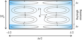
Let us consider a two-dimensional rectangular resonator having rigid walls, which occupies the area defined by  $-L/2 \leqslant \tilde {x} \leqslant L/2$ and
 $-H_0 \leqslant \tilde {y} \leqslant H_0$, as shown in figure 1. The fluid is assumed to be non-Newtonian, whose rheological behaviour obeys Maxwell's model. Excitation of the sound field inside of the microchannel is presumed to be accomplished by a harmonic excitation of a resonator along the
 $\tilde {x}$ axis with velocity
 $v(\tilde {t})$. The microchannel's half-height is
 $H_{0}$, and its length is represented by
 $L$, with
 $L> H_{0}$.
Schematic diagram of the studied physical model. Transversal view of the microchannel.

The basic equations that will form the starting point for studying the oscillatory state of the acoustic flow are the continuity equation,
 \begin{equation} \frac{\partial \tilde{\rho}}{\partial \tilde{t}} + \boldsymbol{\nabla} \boldsymbol{\cdot}\left(\tilde{\rho} \tilde{\boldsymbol{u}}\right)=0, \end{equation}
and the modified Cauchy equation (Hamilton et al. Reference Hamilton, Ilinskii and Zabolotskaya2003a),
 \begin{equation} \tilde{\rho}\left[\frac{\partial \tilde{\boldsymbol{u}}}{\partial \tilde{t}} + \left( \tilde{\boldsymbol{u}} \boldsymbol{\cdot} \boldsymbol{\nabla} \right) \tilde{\boldsymbol{u}} \right] ={-}\boldsymbol{\nabla} \tilde{P} + \boldsymbol{\nabla} \boldsymbol{\cdot} \tilde{\boldsymbol{\tau}}+\boldsymbol{f}. \end{equation}
In (2.2), and following the work by Hamilton, Ilinskii & Zabolotskaya (Reference Hamilton, Ilinskii and Zabolotskaya2002),  $\boldsymbol {f}$ represents an inertial body force. If the resonator vibrates with acceleration
 $\dot {v}(\tilde{t})$ along the
 $\tilde {x}$ axis, the required components of the body force, in
 $\tilde {x}$ and
 $\tilde {y}$ directions, per unit volume on the viscoelastic fluid are
 \begin{equation} f_x ={-}\tilde{\rho} \dot{v}(\tilde{t}), \quad f_y=0, \end{equation}
respectively. It is important to mention that in this work we have adopted the methodology used by Hamilton et al. (Reference Hamilton, Ilinskii and Zabolotskaya2003a) to analyse the acoustic streaming. However, they carried out their study considering a Newtonian fluid.
The equation of state  $\tilde {\rho }=\tilde {\rho }(\tilde {P})$ can be written as (Rednikov & Sadhal Reference Rednikov and Sadhal2011)
 \begin{equation} \frac{\partial \tilde{\rho}}{\partial \tilde{t}}=\frac{1}{c_{0}^{2}} \frac{\partial \tilde{P}}{\partial \tilde{t}}. \end{equation}
The constitutive equation for the stress tensor  $\tilde {\boldsymbol {\tau }}$ in the Cauchy equation, (2.2), corresponds to the Maxwell upper convected model (Tanner Reference Tanner1985), and is given by
 \begin{equation} \tilde{\boldsymbol{\tau}} = 2 \mu \boldsymbol{\mathsf{D}}- \lambda_{1} \left[\frac{\partial \tilde{\boldsymbol{\tau}}}{\partial \tilde{t}} + \left(\tilde{\boldsymbol{u}}\boldsymbol{\cdot} \boldsymbol{\nabla}\right) \tilde{\boldsymbol{\tau}} - \tilde{\boldsymbol{\tau}}\boldsymbol{\cdot}\boldsymbol{\nabla}\tilde{\boldsymbol{u}}- \boldsymbol{\nabla}\tilde{\boldsymbol{u}}^{\rm{T}}\boldsymbol{\cdot} \tilde{\boldsymbol{\tau}} \right]. \end{equation}
In the above (2.1)–(2.5),  $\tilde {\rho }$ is the fluid density,
 $\tilde {\boldsymbol {u}}=(\tilde {u},\tilde {v})$ is the velocity vector,
 $\tilde {P}$ is the acoustic pressure,
 $\tilde {t}$ is the time,
 $\mu$ is the dynamic viscosity of the fluid,
 $\lambda _{1}$ is the fluid relaxation time,
 $\boldsymbol{\mathsf{D}}=(\boldsymbol {\nabla }\tilde {\boldsymbol {u}}+\boldsymbol {\nabla }\tilde {\boldsymbol {u}}^{\rm {T}})/2$ is the rate of deformation tensor,
 $\boldsymbol {\nabla }$ is the nabla operator defined as
 $\boldsymbol {\nabla }\equiv (\partial /\partial \tilde {x}, \partial /\partial \tilde {y})$,
 $\dot {v}(\tilde{t})$ is the derivative with respect of time of the resonator velocity and
 $c_{0}$ is the sound speed inside the fluid.
We assume that the excitation of the resonator is of the form
 \begin{equation} v\left(\tilde{t}\right)=A\omega \exp\left({\rm i}\omega \tilde{t} \right), \end{equation}
where  $A$ is the oscillation amplitude of the resonator,
 $\omega$ is the angular frequency of the resonator and i is the imaginary number,
 ${\rm i}=\sqrt {-1}$.
Equations (2.1)–(2.2) are subject to the following boundary conditions at the microchannel walls:
 \begin{equation} \tilde{\boldsymbol{u}} \boldsymbol{\cdot} \boldsymbol{n}=0 \end{equation}
and
 \begin{equation} \tilde{\boldsymbol{u}} - (\tilde{\boldsymbol{u}} \boldsymbol{\cdot} \boldsymbol{n}) \boldsymbol{n}=0. \end{equation}
Here,  $\boldsymbol {n}$ is the unit vector normal to the surface directed into the fluid. In addition, from symmetry considerations, the velocity component
 $\tilde {u}$ in the
 $\tilde {x}$ direction must be an even function of
 $\tilde {y}$, such that
 $\partial \tilde {u}/\partial \tilde {y}=0$ at
 $\tilde {y}=0$. The velocity component
 $\tilde {v}$ in
 $\tilde {y}$ direction must be an odd function of
 $\tilde {y}$, such that it vanishes at
 $\tilde {y}=0$ (Hamilton et al. Reference Hamilton, Ilinskii and Zabolotskaya2003a).
2.1. Dimensionless mathematical model
Now, we introduce the following dimensionless variables:  $x= 2\tilde {x}/\lambda _{a}$,
 $y= \tilde {y}/H_{0}$,
 $t=\tilde {t}\omega$,
 $\rho =\tilde {\rho }/\rho _{f}$,
 $u=\tilde {u}/A\omega$,
 $v=\tilde {v}/\epsilon A\omega$,
 $P= \tilde {P}/\rho _{f}c_{0}A\omega$ and
 $\boldsymbol {\tau }=\tilde {\boldsymbol {\tau }}H_{0}/\mu A \omega$. Here,
 $\rho _{f}$ is the unperturbed fluid density. The dimensionless form of the governing equations (2.1)–(2.4) are the following:
 \begin{gather} \frac{\partial \rho}{\partial t}={\rm \pi}\eta \frac{\partial P}{\partial t}, \end{gather}
 \begin{gather}\frac{\partial \rho}{\partial t} + \eta \left(\rho\frac{\partial u}{\partial x} + \rho\frac{\partial v}{\partial y} +u\frac{\partial \rho}{\partial x} + v\frac{\partial \rho}{\partial y} \right)=0, \end{gather}
 \begin{gather}\rho\left[\frac{\partial u}{\partial t}+\eta\left(u\frac{\partial u}{\partial x} + v\frac{\partial u}{\partial y} \right)\right]={-}\frac{1}{\rm \pi}\frac{\partial P}{\partial x} + \frac{1}{2\alpha^{2}}\left( \epsilon \frac{\partial \tau_{xx}}{\partial x} + \frac{\partial \tau_{xy}}{\partial y} \right) -{\rm i} \rho \exp({\rm i}t) \end{gather}
and
 \begin{equation} \epsilon^{2}\rho\left[\frac{\partial v}{\partial t}+\eta\left(u\frac{\partial v}{\partial x} + v\frac{\partial v}{\partial y} \right)\right]={-}\frac{1}{\rm \pi}\frac{\partial P}{\partial y} + \frac{\epsilon}{2\alpha^{2}}\left( \epsilon \frac{\partial \tau_{xy}}{\partial x} + \frac{\partial \tau_{yy}}{\partial y} \right). \end{equation}
In the above (2.9)–(2.12),  $\epsilon = 2 H_{0}/\lambda _{a}$ is the ratio between the microchannel height and the wavelength
 $\lambda _{a}$ (
 $\lambda _{a}=2{\rm \pi} c_{0}/\omega$);
 $\alpha =Ho /\delta _{\nu }$, with
 $\delta _{\nu }$ denoting the thickness of the viscous boundary layer (
 $\delta _{\nu }=\sqrt {2\nu /\omega }$),
 $\nu = \mu /\rho _{f}$ and
 $\eta =2A/\lambda _{a}$. The length of the microchannel is chosen as half of the ultrasonic wavelength (
 $L=\lambda _{a}/2$), thereby creating a resonator between both sidewalls of the channel, where a standing wave can be formed (Laurell, Petersson & Nilsson Reference Laurell, Petersson and Nilsson2007).
The dimensionless boundary conditions of (2.9)–(2.12) are as follows:
 \begin{equation} u,v=0 \quad \mathrm{at} \ x={\pm} \tfrac{1}{2} \quad \mathrm{or} \ y={\pm} 1 \end{equation}
and
 \begin{equation} v=0 \quad \mathrm{at} \ y=0. \end{equation}
In addition, the dimensionless components of the constitutive equation (2.5) are
 \begin{gather} \tau_{xx}=2\epsilon\frac{\partial u}{\partial x} - De\left\lbrace\frac{\partial \tau_{xx}}{\partial t} +\eta\left[u\frac{\partial \tau_{xx}}{\partial x} + v\frac{\partial \tau_{xx}}{\partial y} -2\left( \tau_{xx} \frac{\partial u}{\partial x} + \frac{1}{\epsilon}\tau_{xy}\frac{\partial u}{\partial y} \right) \right] \right\rbrace, \end{gather}
 \begin{gather}\tau_{yy}=2\epsilon\frac{\partial v}{\partial y} - De\left\lbrace\frac{\partial \tau_{yy}}{\partial t} +\eta\left[u\frac{\partial \tau_{yy}}{\partial x} + v\frac{\partial \tau_{yy}}{\partial y} -2\epsilon\left( \tau_{xy} \frac{\partial v}{\partial x} + \frac{1}{\epsilon}\tau_{yy}\frac{\partial v}{\partial y} \right) \right] \right\rbrace \end{gather}
and
 \begin{align} \tau_{xy}&=\frac{\partial u}{\partial y} + \epsilon^{2}\frac{\partial v}{\partial x} - De\left \lbrace\frac{\partial \tau_{xy}}{\partial t} +\eta\left[u\frac{\partial \tau_{xy}}{\partial x} + v\frac{\partial \tau_{xy}}{\partial y} - \tau_{xy}\left(\frac{\partial u}{\partial x} + \frac{\partial v}{\partial y}\right) \right. \right. \nonumber\\ &\quad \left. \left. -\frac{1}{\epsilon}\tau_{yy}\frac{\partial u}{\partial y} -\epsilon\tau_{xx}\frac{\partial v}{\partial x} \right] \right\rbrace, \end{align}
where the Deborah number is defined as  $De=\lambda _{1}\omega$. Equations (2.9) to (2.12) are difficult to solve analytically. However, according to typical values of some physical parameters involved in the acoustic field in microfluidics, we can assume that
 $\eta \ll 1$ for
 $A=600\ {\rm nm}$,
 $\lambda =1.578\ {\rm mm}$ and
 $\eta =7.6 \times 10^{-4}$ (Oyama et al. Reference Oyama, Imashiro, Kuriyama, Usui, Ando, Azuma, Morikawa, Kodeki, Takahara and Takemura2021). Therefore, a regular perturbation technique can be used (Bender & Orszag Reference Bender and Orszag2013) to solve the set of mentioned equations, for small values of the number
 $\eta$. Thus, we propose a regular expansion for each dependent variable (say,
 $X$) in the form
 \begin{equation} X=X_0 + \eta X_1+ O(\eta^{2}), \end{equation}
where  $X=u,v,\rho,P,\tau _{ij}$, and we consider that the other dimensionless parameters take values of the order of unity. Substituting the expansion (2.18) into the dimensionless equations (2.9)–(2.17), as well as into the boundary conditions (2.13)–(2.14), and collecting terms of the same order, we obtain the following problems.
At  $O(1)$ we have
 \begin{gather} \frac{\partial \rho_{0}}{\partial t}=0, \end{gather}
 \begin{gather}\rho_{0}\frac{\partial u_{0}}{\partial t}={-}\frac{1}{\rm \pi}\frac{\partial P_{0}}{\partial x} + \frac{1}{2\alpha^{2}}\left( \epsilon \frac{\partial \tau_{xx0}}{\partial x} + \frac{\partial \tau_{xy0}}{\partial y} \right) -{\rm i} \rho_{0} \exp({\rm i}t), \end{gather}
 \begin{gather}\epsilon^{2}\rho_{0}\frac{\partial v_{0}}{\partial t}={-}\frac{1}{\rm \pi}\frac{\partial P_{0}}{\partial y} + \frac{\epsilon}{2\alpha^{2}}\left( \epsilon \frac{\partial \tau_{xy0}}{\partial x} + \frac{\partial \tau_{yy0}}{\partial y} \right). \end{gather}
At the leading order, the state and continuity equations take the same form of (2.19), and it shows that the zero-order solution of the dimensionless density is independent of time, given by
 \begin{equation} \rho_{0}=\rho^{{\ast}}, \end{equation}
where  $\rho ^{\ast }$ is a constant, and corresponds to the condition of the unperturbed system
 $\rho ^{\ast }=1$. Since the zero-order solution of the dimensionless density does not fully describe the mass transport in the microchannel, we substitute (2.9) into (2.10), to obtain a modified zero-order continuity equation as follows:
 \begin{equation} {\rm \pi}\frac{\partial P_{0}}{\partial t} + \frac{\partial u_{0}}{\partial x} + \frac{\partial v_{0}}{\partial y}=0, \end{equation}
as well as modifying (2.20) and (2.21) using (2.22), to give
 \begin{gather} \frac{\partial u_{0}}{\partial t}={-}\frac{1}{\rm \pi}\frac{\partial P_{0}}{\partial x} + \frac{1}{2\alpha^{2}}\left( \epsilon \frac{\partial \tau_{xx0}}{\partial x} + \frac{\partial \tau_{xy0}}{\partial y} \right)-{\rm i} \exp({\rm i}t), \end{gather}
 \begin{gather}\epsilon^{2}\frac{\partial v_{0}}{\partial t}={-}\frac{1}{\rm \pi}\frac{\partial P_{0}}{\partial y} + \frac{ \epsilon}{2\alpha^{2}}\left( \epsilon \frac{\partial \tau_{xy0}}{\partial x} + \frac{\partial \tau_{yy0}}{\partial y} \right). \end{gather}
Concerning the required boundary conditions of the acoustic pressure  $P$, the design configuration of half-wavelength resonator yields an acoustic pressure node in the centre of the microchannel, i.e.
 $P=0$ at
 $x=0$. Therefore, the above will be used as a boundary condition for the pressure field. Furthermore, the boundary conditions of the set of (2.24)–(2.25) are
 \begin{equation} u_{0},v_{0}=0 \quad \mathrm{at} \ x={\pm} \tfrac{1}{2} \quad \mathrm{or} \ y={\pm} 1 \end{equation}
and
 \begin{equation} v_{0}=0 \quad \mathrm{at} \ y=0. \end{equation}
The zero-order components of the constitutive equations (2.15)–(2.17) are given by
 \begin{gather} \tau_{xx0}=2\epsilon\frac{\partial u_{0}}{\partial x} - De\frac{\partial \tau_{xx0}}{\partial t}, \end{gather}
 \begin{gather}\tau_{yy0}=2\epsilon\frac{\partial v_{0}}{\partial y} - De\frac{\partial \tau_{yy0}}{\partial t} \end{gather}
and
 \begin{equation} \tau_{xy0}=\frac{\partial u_{0}}{\partial y} + \epsilon^{2}\frac{\partial v_{0}}{\partial x} - De\frac{\partial \tau_{xy0}}{\partial t}. \end{equation}
To solve the previous equations at  $O(1)$, we propose a periodic solution that ignores the transient stage, stipulating that the dependence on the time is carried out through an oscillating behaviour. We assume a solution for each dependent variable of the form
 \begin{equation} (u_{0},v_{0},P_{0},\boldsymbol{\tau}_{0})=\mathrm{Im}\left[\left ( U(x,y),V(x,y),\hat{P}(x,y),\varXi(x,y) \right) \exp({\rm i}t) \right]. \end{equation}
Substituting (2.31) into (2.28)–(2.30) yields
 \begin{gather} \varXi_{xx}=\frac{2\epsilon}{\sigma} \frac{\partial U}{\partial x}, \end{gather}
 \begin{gather}\varXi_{yy}=\frac{2\epsilon}{\sigma} \frac{\partial V}{\partial y}, \end{gather}
 \begin{gather}\varXi_{xy}=\frac{1}{\sigma}\left(\frac{\partial U}{\partial y} +\epsilon^{2}\frac{\partial V}{\partial x} \right), \end{gather}
respectively, where
 \begin{equation} \sigma=1+{\rm i} De. \end{equation}
In the same manner, substituting (2.31) into the governing equations (2.23)–(2.25), we obtain the leading order for those equations as follows:
 \begin{gather} {\rm i}{\rm \pi}\hat{P} + \frac{\partial U}{\partial x} + \frac{\partial V}{\partial y}=0, \end{gather}
 \begin{gather}{\rm i} U={-}\frac{1}{\rm \pi}\frac{\partial \hat{P}}{\partial x} + \frac{1}{2\alpha^{2}}\left( \epsilon \frac{\partial \varXi_{xx}}{\partial x} + \frac{\partial \varXi_{xy}}{\partial y} \right)-{i}, \end{gather}
 \begin{gather}{\rm i}\epsilon^{2}V={-}\frac{1}{\rm \pi}\frac{\partial \hat{P}}{\partial y} + \frac{1}{2\alpha^{2}}\left( \epsilon^{2} \frac{\partial \varXi_{xy}}{\partial x} + \epsilon\frac{\partial \varXi_{yy}}{\partial y} \right). \end{gather}
The associated boundary conditions of (2.36)–(2.38) are
 \begin{gather} U,V=0 \quad \mathrm{at} \ x={\pm} \tfrac{1}{2} \quad \mathrm{or} y={\pm} 1, \end{gather}
 \begin{gather}V=0 \quad \mathrm{at} \ y=0 \end{gather}
and
 \begin{equation} \hat{P}=0 \quad \mathrm{at} \ x=0. \end{equation}
2.2. Simplified governing equations
Combining (2.32)–(2.34) with (2.37)–(2.38) the following set of equations is obtained:
 \begin{gather} {\rm i} U={-}\frac{1}{\rm \pi}\frac{\partial \hat{P}}{\partial x} + \frac{1}{2\alpha^{2}}\left[ \frac{2\epsilon^{2}}{\sigma} \frac{\partial^{2} U}{\partial x^{2}} +\frac{1}{\sigma}\left( \frac{\partial^{2} U}{\partial y^{2}} +\epsilon^{2}\frac{\partial^{2} V}{\partial x \partial y} \right)\right]-{i}, \end{gather}
 \begin{gather}{\rm i}\epsilon^{2}V={-}\frac{1}{\rm \pi}\frac{\partial \hat{P}}{\partial y} + \frac{1}{2\alpha^{2}}\left[ \frac{\epsilon^{2}}{\sigma}\left(\frac{\partial^{2} U}{\partial x \partial y} +\epsilon^{2}\frac{\partial^{2} V}{\partial x^{2}} \right) + \frac{2\epsilon^{2}}{\sigma}\frac{\partial^{2} V}{\partial y^{2}} \right]. \end{gather}
By considering the values of the physical parameters  $H_{0}=20\delta _{\nu }=21\ \mathrm {\mu }{\rm m}$ and
 $\lambda _{a}=1.578$ mm, we get that
 $\epsilon \sim O(10^{-2})$ (Hamilton et al. Reference Hamilton, Ilinskii and Zabolotskaya2003a; Oyama et al. Reference Oyama, Imashiro, Kuriyama, Usui, Ando, Azuma, Morikawa, Kodeki, Takahara and Takemura2021). Therefore, in (2.42)–(2.43) we can neglect terms that are proportional to
 $\epsilon ^2$, and thus, that equations can be simplified as follows:
 \begin{gather} \frac{\rm \pi}{2\alpha^{2}\sigma}\frac{\partial^{2} U}{\partial y^{2}}-{\rm i}{\rm \pi} U= \frac{\partial \hat{P}}{\partial x} +{\rm i}{\rm \pi}, \end{gather}
 \begin{gather}\frac{\partial \hat{P}}{\partial y}=0. \end{gather}
From the above equation,  $\hat {P}=\hat {P}(x)$. To solve (2.36) and (2.44)–(2.45) we follow the procedure proposed by Hamilton et al. (Reference Hamilton, Ilinskii and Zabolotskaya2003a). Therefore, we introduce the following function:
 \begin{equation} U_{x}(x)=\frac{{\rm d} \hat{P}}{{\rm d} x}+{\rm i} {\rm \pi}, \end{equation}
into (2.44). The general solution of (2.44), taking into account the no-slip boundary condition ( $U=0 \ \mathrm {at} \ y=\pm 1$), is
 \begin{equation} U(x,y)=\frac{U_{x}(x)}{{\rm i}{\rm \pi}}\left[\frac{\cosh(\zeta y)}{\cosh({\zeta})}-1 \right], \end{equation}
where
 \begin{equation} \zeta =\alpha \sqrt{2 \left({\rm i}- De \right)}. \end{equation}
Equation (2.47) is similar to that obtained by Hamilton et al. (Reference Hamilton, Ilinskii and Zabolotskaya2003a). However, in our case, that equation involves the parameter  $\zeta$, defined in (2.48), which shows the viscoelastic effect represented in the Deborah number
 $De$. Evidently, when
 $De=0$, the solution obtained by Hamilton et al. (Reference Hamilton, Ilinskii and Zabolotskaya2003a) is recovered. In (2.47) we still need to determine the
 $x$ dependence. To this end we introduce the average axial velocity defined by (Hamilton et al. Reference Hamilton, Ilinskii and Zabolotskaya2003a)
 \begin{equation} \bar{U}(x)=\tfrac{1}{2}\int_{{-}1}^{1} U(x,y)\,{{\rm d} y}. \end{equation}
Accordingly, substituting (2.47) into (2.49), we obtain
 \begin{equation} \bar{U}(x)=\frac{U_{x}(x)}{{\rm i}{\rm \pi}}\left(f_{\nu} -1 \right), \end{equation}
where
 \begin{equation} f_{\nu}=\frac{\tanh(\zeta )}{\zeta }. \end{equation}
From (2.50) we have an equation that relates the average axial velocity with  $U_{x}(x)$. Combining (2.47) and (2.50), we obtain
 \begin{equation} U(x,y)=\frac{\bar{U}(x)}{1-f_{\nu}}\left[1-\frac{\cosh(\zeta y)}{\cosh({\zeta})} \right]. \end{equation}
Similarly, averaging (2.36) and (2.44) in the  $y$ direction yields
 \begin{equation} -\frac{1}{{\rm i}{\rm \pi}}\frac{{\rm d} \bar{U}(x)}{{\rm d} x}= \hat{P} \end{equation}
and
 \begin{equation} {\rm i} \sigma {\rm \pi}\bar{U}(x)+\sigma \frac{{\rm d} \hat{P}}{{\rm d} x}={-}{\rm i} \sigma {\rm \pi}\left.+\frac{\rm \pi}{4\alpha^{2}} \frac{\partial U(x,y)}{\partial y} \right\vert_{{-}1}^{1}, \end{equation}
respectively. We differentiate (2.52) with respect to  $y$, evaluating at
 $y = -1$ and
 $y=1$, to obtain the last term from the right side of (2.54) as follows:
 \begin{equation} \left.\frac{\rm \pi}{4\alpha^{2}} \frac{\partial U(x,y)}{\partial y} \right\vert_{{-}1}^{1}= {\rm i} \sigma {\rm \pi}\frac{f_{\nu} \bar{U}(x)}{f_{\nu}-1}, \end{equation}
and (2.54) becomes
 \begin{equation} \frac{ \bar{U}(x)}{f_{\nu}-1}=\frac{1}{{\rm i}{\rm \pi}}\frac{{\rm d} \hat{P}}{{\rm d} x}+1. \end{equation}
Combining (2.53) and (2.56) yields
 \begin{equation} \frac{{\rm d}^{2} \bar{U}(x)}{{{\rm d} x}^{2}}-\xi^{2}\bar{U}(x)={-}\xi^{2}\left(f_{\nu}-1 \right), \end{equation}
where
 \begin{equation} \xi=\frac{\rm \pi}{(f_{\nu}-1)^{1/2}}. \end{equation}
The solution of (2.57), considering the boundary condition  $U=0$ at
 $x=\pm 1/2$, is given by
 \begin{equation} \bar{U}(x)=(f_{\nu}-1)\left[ 1 - \frac{\cosh(\xi x)}{\cosh(\xi/2)} \right], \end{equation}
and, therefore, introducing (2.59) into (2.52), the axial component of the particle velocity becomes
 \begin{equation} U(x,y)= \left[ 1 - \frac{\cosh(\xi x)}{\cosh(\xi/2)} \right]\left[\frac{\cosh(\zeta y)}{\cosh({\zeta})}-1 \right]. \end{equation}
From (2.53) and (2.59) we obtain the acoustic pressure, that satisfies (2.41), as follows:
 \begin{equation} \hat{P}(x)={-}\frac{{\rm i} {\rm \pi}}{\xi}\frac{\sinh(\xi x)}{\cosh(\xi/2)}. \end{equation}
Finally, to determine the transverse velocity component, we integrate (2.36) with respect to  $y$, from
 $0$ to
 $y$, noting that
 $V=0$ at
 $y=0$, as follows:
 \begin{equation} V(x,y)={-}{\rm i}{\rm \pi} \hat{P} y - \int_{0}^{y}\frac{\partial U}{\partial x}{{\rm d} y}. \end{equation}
Substitution of (2.60) and (2.61) into (2.62), yields
 \begin{equation} V=\xi f_{\nu}\frac{\sinh(\xi x)}{\cosh(\xi/2)}\left[\frac{\sinh(\zeta y)}{\sinh({\zeta })}-y\right] . \end{equation}
At this order in the asymptotic analysis, it should be noted that  $V$ cannot satisfy the boundary conditions at
 $x=\pm 1/2$. The above is a consequence of neglecting viscous terms in the momentum equations (2.42) and (2.43), which are affected by terms of
 $O(\varepsilon ^2)$. From these equations, it is evident the existence of boundary-layers near to
 $x= \pm 1/2$. While it has been shown that the thickness of these boundary layers increase with
 $De$ (Bird, Armstrong & Hassager Reference Bird, Armstrong and Hassager1987; Ortín Reference Ortín2019), the influence of these layers in both ends represent a small correction to the system's response with the parameters used in this work.
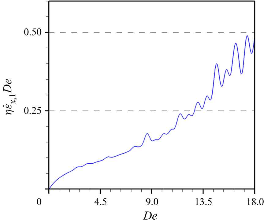
In addition to the aforementioned, it is known that the upper convected Maxwell model has a limitation that makes the product of extensional rate  $\dot {\tilde {\varepsilon }}=(\dot {\tilde {\varepsilon }}_{x},\dot {\tilde {\varepsilon }}_{y} )$ times the relaxation time
 $\lambda _{1}$ be less than one half, i.e.
 $\dot {\tilde {\varepsilon }}_{x,y} \lambda _{1}\ll 1/2$ (Macosko Reference Macosko1994). The following dimensionless equations are the components of the extensional rate in the
 $x$ and
 $y$ directions at
 $O(\eta )$:
 \begin{equation} \dot{\varepsilon}_{x}= \frac{\partial U}{\partial x} \end{equation}
and
 \begin{equation} \dot{\varepsilon}_{y}= \frac{\partial V}{\partial y}, \end{equation}
with  $\dot {\varepsilon }_{x,y}=\dot {\tilde {\varepsilon }}_{x,y}/\omega$. In terms of the dimensionless parameters used in this work,
 $\dot {\tilde {\varepsilon }}_{x,y} \lambda _{1}=\dot {\varepsilon }_{x,y}De\ll 1/2$. To calculate the maximum value that
 $\dot {\varepsilon }_{x,y}De$ can attain, we use the velocity field, given by (2.60) and (2.63), together with (2.64) and (2.65). After the calculations, we found that the maximum extensional rate, at
 $O(\eta )$, is only controlled by the values of
 $\dot {\varepsilon }_x$. Such a maximum value is estimated for
 $De \approx 18$, from which the condition
 $\dot {\varepsilon } De <0.5$ is satisfied, as can be seen in figure 2. In terms of the perturbation expansions, the condition that must be satisfied is given by
 $(\dot {\varepsilon }_{x,0} +\eta \dot {\varepsilon }_{x,1} + O(\eta ^2)) De <0.5$, where
 $\dot {\varepsilon }_{x,0} =0$. In this work, we have used
 $De=10$ as the intermediate limit for the calculation shown in § 4.
Real values of  $\eta \dot {\varepsilon }_{x,1} De$ for different values of
 $De$. Here,
 $\alpha =20$.

At this point, we have obtained the zero-order solution for the velocity components  $u_0=\mathrm {Im}[ U(x,y) \exp ({\rm i} t )]$ and
 $v_0=\mathrm {Im}[ V(x,y) \exp ({\rm i} t ) ]$, as well as for the pressure field
 $P_0=\mathrm {Im}[ \hat {P}( x) \exp ({\rm i} t ) ]$. The next step is to evaluate the solutions at
 $O(\eta )$ for
 $u_1$ and
 $v_1$. However, if we apply the conventional scheme that was used to obtain the order-zero solution, we find that such a task is difficult because the first-order continuity equation will disappear when the time average of (2.10) is carried out; another option is to introduce (2.9) into (2.10) and then take its time average, but the resulting equation takes the form of a first-order partial differential equation that cannot satisfy all the boundary conditions. Either way, what is left behind is only the
 $x$ component momentum equation to determine the principal unknowns (
 $u_{1},v_{1}$). Therefore, we proceed to obtain the solution at
 $O(\eta )$ by using the vorticity (
 $\varOmega _1$) stream function (
 $\psi _1$) formulation as shown in § 3. Here, the subscript
 $1$ indicates the solution at
 $O(\eta )$ for the vorticity and stream function, and the results obtained in the present section will be useful in § 3.
3. Secondary steady flow
Before we carry out the time average of the governing equations to obtain the solution of the first order for the unknown variables  $u_{1}$ and
 $v_{1}$, we start this section by introducing the dimensionless version of the unsteady compressible stream function
 $\tilde {\psi }$ and vorticity,
 $\tilde {\varOmega }$, defined as follows (Yalamanchili & Benzkofer Reference Yalamanchili and Benzkofer1973; White Reference White2006):
 \begin{equation} \rho u=\frac{\partial \psi}{\partial y}, \quad \rho v={-}\left(\frac{\partial \psi}{\partial x}+ \frac{\partial \bar{y}}{\partial t} \right), \end{equation}
where
 \begin{equation} \bar{y}={\rm \pi}\int_{0}^{y}P(x,y,t)\,{{\rm d} y} \end{equation}
and
 \begin{equation} \varOmega =\epsilon^{2} \frac{\partial v}{\partial x} -\frac{\partial u}{\partial y}, \end{equation}
with  $\psi = \tilde {\psi }/A\omega H_{0}$ and
 $\varOmega =\tilde {\varOmega } H_{0}/A\omega$. Here,
 $\tilde {\psi }$ and
 $\tilde {\varOmega }$ represent the stream function and vorticity in physical units. The next step is to take the curl of the momentum equations with the aim of replacing the components of the dimensionless particle velocity
 $\boldsymbol {u}=(u,v)$ with the vorticity
 $\varOmega$. This process can be achieved if we differentiate the
 $x$ component of the momentum equations with respect to
 $y$ coordinate, and the
 $y$ component of the momentum equations is differentiated with respect to
 $x$ coordinate, where the latter resulting equation is subtracted from the former. Therefore, we differentiate (2.24) with respect to
 $y$, and (2.25) is differentiated with respect to
 $x$, obtaining
 \begin{align} &\rho\frac{\partial^{2} u}{\partial y\partial t}+ \frac{\partial \rho}{\partial y}\frac{\partial u}{\partial t}+\eta\left[\left(\rho \frac{\partial u}{\partial y}+u\frac{\partial \rho}{\partial y}\right)\frac{\partial u}{\partial x} + \rho u \frac{\partial^{2} u}{\partial x \partial y} +\left(\rho \frac{\partial v}{\partial y}+ v \frac{\partial \rho}{\partial y}\right)\frac{\partial u}{\partial y} +\rho v\frac{\partial^{2} u}{\partial y^{2}}\right] \nonumber\\ &\quad ={-}\frac{1}{\rm \pi}\frac{\partial^{2} P}{\partial x \partial y} + \frac{1}{2\alpha^{2}}\left( \epsilon \frac{\partial^{2} \tau_{xx}}{\partial x\partial y} + \frac{\partial^{2} \tau_{xy}}{\partial y^{2}} \right)-\frac{\partial \rho}{\partial y}\dot{v}(t) \end{align}
and
 \begin{align} &\epsilon^{2}\left(\rho\frac{\partial^{2} v}{\partial x \partial t}+\frac{\partial \rho}{\partial x}\frac{\partial v}{ \partial t}\right)+\epsilon^{2}\eta\left[\left(\rho \frac{\partial u}{\partial x}+u\frac{\partial \rho}{\partial x}\right)\frac{\partial v}{\partial x} +\rho u \frac{\partial^{2} v}{\partial x^{2}} +\left(\rho \frac{\partial v}{\partial x}+v\frac{\partial \rho}{\partial x}\right)\frac{\partial v}{\partial y} \right. \nonumber\\ &\left.\quad+\,\rho v \frac{\partial^{2} v}{\partial x \partial y}\right] ={-}\frac{1}{\rm \pi}\frac{\partial^{2} P}{\partial x\partial y} + \frac{1}{2\alpha^{2}}\left( \epsilon^{2} \frac{\partial^{2} \tau_{xy}}{\partial x^{2}} + \epsilon\frac{\partial^{2} \tau_{yy}}{\partial x \partial y} \right), \end{align}
respectively. Subtracting (3.5) from (3.4), and using (3.3), yields the following equation:
 \begin{align} &\varOmega \frac{\partial \rho}{\partial t} - \rho \frac{\partial \varOmega}{\partial t} + \frac{\partial \rho}{\partial y}\frac{\partial u}{\partial t}-\epsilon^{2} \frac{\partial \rho}{\partial x}\frac{\partial v}{\partial t}\nonumber\\ &\qquad -\eta\left[\rho u \frac{\partial \varOmega}{\partial x} \!+\! \rho v \frac{\partial \varOmega}{\partial y} -\frac{\partial \rho}{\partial x}\left( u \varOmega -\epsilon^{2} u \frac{\partial v}{\partial x}-\epsilon^{2} v \frac{\partial v}{\partial y}\right) -\frac{\partial \rho}{\partial y}\left(u \frac{\partial u}{\partial x} \!+\!v\frac{\partial u}{\partial y} +\!v \varOmega\right) \right] \nonumber\\ &\quad ={-}\frac{\partial \rho}{\partial y}\dot{v}(t)+\frac{1}{2 \alpha^{2}}\left[\epsilon\left(\frac{\partial^{2} \tau_{xx}}{\partial x \partial y} - \frac{\partial \tau_{yy}}{\partial x \partial y}\right) -\epsilon^{2} \frac{\partial ^{2} \tau_{xy}}{\partial x^{2}}+\frac{\partial^{2} \tau_{xy}}{\partial y^{2}} \right] . \end{align}
The next step is to expand the stress tensor components in (3.6) using (2.15)–(2.17), obtaining the following equation:
 \begin{align} &\frac{\partial^{2}
\varOmega}{\partial y^{2}}+\epsilon^{2}\frac{\partial^{2}
\varOmega}{\partial x^{2}} +2\alpha^{2}
\left(\varOmega\frac{\partial \rho}{\partial t} - \rho
\frac{\partial \varOmega}{\partial
t}\right)+2\alpha^{2}\left[\frac{\partial \rho}{\partial
y}\left(\frac{\partial u}{\partial
t}+\dot{v}(t)\right)-\epsilon^{2}\frac{\partial
\rho}{\partial x}\frac{\partial v}{\partial t}\right]
\nonumber\\ &\quad =2\alpha^{2}\eta\left[\rho u
\frac{\partial \varOmega}{\partial x} +\rho v
\frac{\partial \varOmega}{\partial y} -\frac{\partial
\rho}{\partial x}\left( u \varOmega -\epsilon^{2} u
\frac{\partial v}{\partial x}-\epsilon^{2} v \frac{\partial
v}{\partial y}\right)\right.\nonumber\\ &\qquad
\left.-\frac{\partial \rho}{\partial y}\left(u
\frac{\partial u}{\partial x} +v\frac{\partial u}{\partial
y} +v \varOmega\right)\right] -De\frac{\partial}{\partial
t}\left[\epsilon\left(\frac{\partial^{2}
\tau_{xx}}{\partial x \partial y} - \frac{\partial
\tau_{yy}}{\partial x \partial y}\right)-\epsilon^{2}
\frac{\partial ^{2} \tau_{xy}}{\partial
x^{2}}+\frac{\partial^{2} \tau_{xy}}{\partial y^{2}}\right]
\nonumber\\ &\qquad -\eta De\left[ \epsilon
u\left(\frac{\partial ^{3} \tau_{xx}}{\partial x^{2}
\partial y}-\frac{\partial^{3} \tau_{yy}}{\partial x^{2}
\partial y} -\epsilon \frac{\partial^{3}
\tau_{xy}}{\partial x^{3}}+\frac{1}{\epsilon}\frac{\partial
^{3} \tau_{xy}}{\partial x \partial y^{2}}\right) \right.
\nonumber\\ &\left. \qquad +\, \epsilon
v\left(\frac{\partial^{3} \tau_{xx}}{\partial x \partial
y^{2}} - \frac{\partial^{3} \tau_{yy}}{\partial x \partial
y^{2}} -\epsilon \frac{\partial ^{3} \tau_{xy}}{\partial
x^{2} \partial y} +\frac{1}{\epsilon} \frac{\partial^{3}
\tau_{xy}}{\partial y^{3}}\right) \right.\nonumber\\
&\qquad - \epsilon \frac{\partial u}{\partial
x}\left(\frac{\partial^{2} \tau_{xx}}{\partial x \partial
y} + \frac{\partial^{2} \tau_{yy}}{\partial x \partial y} +
\epsilon \frac{\partial^{2} \tau_{xy}}{\partial
x^{2}}+\frac{1}{\epsilon}\frac{\partial^{2}
\tau_{xy}}{\partial y^{2}} \right) \nonumber\\ &\qquad
+\epsilon \frac{\partial u}{\partial
y}\left(\frac{\partial^{2} \tau_{xx}}{\partial x^{2}}
-\frac{1}{\epsilon^{2}}\frac{\partial^{2}
\tau_{yy}}{\partial y^{2}} \right) +\epsilon
\frac{\partial^{2} u}{\partial x \partial
y}\left(-\frac{\partial \tau_{xx}}{\partial x} -
\frac{4}{\epsilon}\frac{\partial \tau_{xy}}{\partial y}
+\frac{\partial \tau_{yy}}{\partial x} \right) \nonumber\\
&\qquad +\epsilon \frac{\partial^{2} u}{\partial
x^{2}}\left({-}2 \frac{\partial \tau_{xx}}{\partial y}
+\epsilon \frac{\partial \tau_{xy}}{\partial x}\right)
-\frac{\partial^{2} u}{\partial y^{2}}\left(\frac{\partial
\tau_{xy}}{\partial x} +\frac{2}{\epsilon}\frac{\partial
\tau_{yy}}{\partial y}\right) + \epsilon
\frac{\partial^{3} u}{\partial x^{2} \partial
y}\left(\tau_{yy}-2\tau_{xx}\right) \nonumber\\ &\qquad
-3\frac{\partial^{3} u}{\partial x \partial y^{2}}
\tau_{xy}-\epsilon \frac{\partial v}{\partial
x}\left(\frac{\partial^{2} \tau_{yy}}{\partial
y^{2}}-\epsilon^{2} \frac{\partial^{2} \tau_{xx}}{\partial
x^{2}} \right) +\epsilon\frac{\partial v}{\partial
y}\left(\frac{\partial^{2} \tau_{xx}}{\partial x \partial
y}+ \frac{\partial^{2} \tau_{yy}}{\partial x \partial
y}\right.\nonumber\\ &\qquad +\epsilon \frac{\partial^{2}
\tau_{xy}}{\partial x^{2}} -\epsilon \tau_{xy}
\left.+\frac{1}{\epsilon} \frac{\partial ^{2}
\tau_{xy}}{\partial y^{2}}
\right)+\epsilon\frac{\partial^{2} v}{\partial x \partial
y}\left(\frac{\partial \tau_{yy}}{\partial y}+4\epsilon
\frac{\partial \tau_{xy}}{\partial x}-\frac{\partial
\tau_{xx}}{\partial y}\right) \nonumber\\ &\qquad
+\epsilon^{2} \frac{\partial^{2} v}{\partial
x^{2}}\left(\frac{\partial \tau_{xy}}{\partial y}
+2\epsilon \frac{\partial \tau_{xx}}{\partial x} \right)
+2\epsilon\frac{\partial^{2} v}{\partial
y^{2}}\left(\frac{\partial \tau_{yy}}{\partial x}
-\frac{1}{2\epsilon }\frac{\partial \tau_{xy}}{\partial y}
\right) \nonumber\\ &\qquad
+3\epsilon^{2}\frac{\partial^{3} v}{\partial x^{2} \partial
y}\tau_{xy}+2\epsilon\frac{\partial ^{3} v}{\partial x
\partial y^{2}} \tau_{yy} +\epsilon^{2} \left(
\frac{\partial ^{3} u}{\partial x^{3}} \tau_{xy}
+\frac{\partial ^{3} v}{\partial x^{3}}\tau_{xx}
\right)\nonumber\\ &\qquad
\left.-\left(\frac{1}{\epsilon}\frac{\partial^{3}
u}{\partial y^{3}}\tau_{yy} + \frac{\partial^{3}
v}{\partial y^{3}} \tau_{xy} \right) \right].
\end{align}
As previously discussed  $\epsilon \sim O(10^{-2})$, thus we neglected terms in (3.7) that are proportional to
 $\epsilon$, simplifying it as follows:
 \begin{align} &\frac{\partial^{2} \varOmega}{\partial y^{2}}+2\alpha^{2}\left[ \left(\varOmega\frac{\partial \rho}{\partial t} - \rho \frac{\partial \varOmega}{\partial t}\right)+\frac{\partial \rho}{\partial y}\left(\frac{\partial u}{\partial t}+\dot{v}(t)\right) \right]\nonumber\\ &\quad = 2\alpha^{2}\eta\left[\rho u \frac{\partial \varOmega}{\partial x} +\rho v \frac{\partial \varOmega}{\partial y} -\frac{\partial \rho}{\partial x} u \varOmega -\frac{\partial \rho}{\partial y}\left(u \frac{\partial u}{\partial x} +v\frac{\partial u}{\partial y} +v \varOmega\right)\right] \nonumber\\ &\qquad -De\frac{\partial^{3} \tau_{xy}}{\partial y^{2}\partial t}-\eta De\left( u\frac{\partial ^{3} \tau_{xy}}{\partial x \partial y^{2}} +v \frac{\partial^{3} \tau_{xy}}{\partial y^{3}} -\frac{\partial u}{\partial x}\frac{\partial^{2} \tau_{xy}}{\partial y^{2}} \right. \nonumber\\ &\qquad \left.-\frac{1}{\epsilon}\frac{\partial u}{\partial y}\frac{\partial^{2} \tau_{yy}}{\partial y^{2}} - 4\frac{\partial^{2} u}{\partial x \partial y}\frac{\partial \tau_{xy}}{\partial y} -\frac{\partial^{2} u}{\partial y^{2}}\frac{\partial \tau_{xy}}{\partial x} -\frac{2}{\epsilon}\frac{\partial^{2} u}{\partial y^{2}}\frac{\partial \tau_{yy}}{\partial y} -3\frac{\partial^{3} u}{\partial x \partial y^{2}} \tau_{xy} +\frac{\partial v}{\partial y} \frac{\partial ^{2} \tau_{xy}}{\partial y^{2}} \right. \nonumber\\ &\qquad \left. -\frac{\partial^{2} v}{\partial y^{2}}\frac{\partial \tau_{xy}}{\partial y}-\frac{1}{\epsilon}\frac{\partial^{3} u}{\partial y^{3}}\tau_{yy} - \frac{\partial^{3} v}{\partial y^{3}} \tau_{xy} \right) +O(\epsilon). \end{align}
As mentioned at the end of § 2, to determine the acoustic streaming we need the first-order solution of (3.1a,b), (3.3) and (3.8). Therefore, we present its first-order solutions as follows.
At  $O(\eta )$ we have
 \begin{gather} u_{1} + \rho_{1} u_{0}=\frac{\partial \psi_{1}}{\partial y}, \end{gather}
 \begin{gather}\varOmega_{1} ={-}\frac{\partial u_{1}}{\partial y}+O(\epsilon^{2}) \end{gather}
and
 \begin{align} &\frac{\partial^{2} \varOmega_{1}}{\partial y^{2}}+2\alpha^{2}\left[\varOmega_{0}\frac{\partial \rho_{1}}{\partial t} - \rho_{1} \frac{\partial \varOmega_{0}}{\partial t}- \frac{\partial \varOmega_{1}}{\partial t}+\frac{\partial \rho_{1}}{\partial y}\left(\frac{\partial u_{0}}{\partial t}+\dot{v}(t)\right) \right]\nonumber\\ &\quad = 2\alpha^{2}\left( u_{0} \frac{\partial \varOmega_{0}}{\partial x} + v_{0} \frac{\partial \varOmega_{0}}{\partial y} \right)- De\left(\frac{\partial^{3} \tau_{xy1}}{\partial y^{2}\partial t}+ u_{0}\frac{\partial ^{3} \tau_{xy0}}{\partial x \partial y^{2}} +v_{0} \frac{\partial^{3} \tau_{xy0}}{\partial y^{3}} \right.\nonumber\\ &\qquad -\frac{\partial u_{0}}{\partial x}\frac{\partial^{2} \tau_{xy0}}{\partial y^{2}} -\frac{1}{\epsilon}\frac{\partial u_{0}}{\partial y}\frac{\partial^{2} \tau_{yy0}}{\partial y^{2}} - 4\frac{\partial^{2} u_{0}}{\partial x \partial y}\frac{\partial \tau_{xy0}}{\partial y} -\frac{\partial^{2} u_{0}}{\partial y^{2}} \frac{\partial \tau_{xy0}}{\partial x} -\frac{2}{\epsilon }\frac{\partial^{2} u_{0}}{\partial y^{2}} \frac{\partial \tau_{yy0}}{\partial y}\nonumber\\ &\qquad -3\frac{\partial^{3} u_{0}}{\partial x \partial y^{2}} \tau_{xy0} \left.+\frac{\partial v_{0}}{\partial y} \frac{\partial ^{2} \tau_{xy0}}{\partial y^{2}} -\frac{\partial^{2} v_{0}}{\partial y^{2}}\frac{\partial \tau_{xy0}}{\partial y}-\frac{1}{\epsilon}\frac{\partial^{3} u_{0}}{\partial y^{3}}\tau_{yy0} - \frac{\partial^{3} v_{0}}{\partial y^{3}} \tau_{xy0} \right) +O(\epsilon). \end{align}
Finally, we introduce (3.9) into (3.10), and substitute the zero-order stress tensor terms in (3.11) using (2.32)–(2.34), obtaining
 \begin{align} &\varOmega_{1} ={-}\frac{\partial^{2} \psi_{1}}{\partial y^{2}}+\rho_{1}\frac{\partial u_{0}}{\partial y}+u_{0}\frac{\partial \rho_{1}}{\partial y}+O(\epsilon^{2}), \end{align}
 \begin{align} &\frac{\partial^{2} \varOmega_{1}}{\partial y^{2}}+2\alpha^{2}\left[\varOmega_{0}\frac{\partial \rho_{1}}{\partial t} - \rho_{1} \frac{\partial \varOmega_{0}}{\partial t}- \frac{\partial \varOmega_{1}}{\partial t}+\frac{\partial \rho_{1}}{\partial y}\left(\frac{\partial u_{0}}{\partial t}+\dot{v}(t)\right) \right] \nonumber\\ &\quad =2\alpha^{2}\left( u_{0} \frac{\partial \varOmega_{0}}{\partial x} + v_{0} \frac{\partial \varOmega_{0}}{\partial y} \right)-De\frac{\partial^{3} \tau_{xy1}}{\partial y^{2}\partial t}- \frac{De}{\sigma}\left[u_{0}\frac{\partial^{4} u_{0}}{\partial x \partial y^{3}} +v_{0}\frac{\partial^{4} u_{0}}{\partial y^{4}} -\frac{\partial u_{0}}{\partial x}\frac{\partial^{3} u_{0}}{\partial y^{3}} \right. \nonumber\\ &\qquad \left.-\left(5\frac{\partial^{2} u_{0}}{\partial y^{2}}+3\frac{\partial u_{0}}{\partial y}\frac{\partial }{\partial y}\right)\left(\frac{\partial^{2} v_{0}}{\partial y^{2}} + \frac{\partial ^{2} u_{0}}{\partial x \partial y} \right) \right] +O(\epsilon). \end{align}
Equation (3.13) can be simplified since the second and third left-hand terms are equal in magnitude but opposite ( ${\rm i} \rho _{1}\varOmega _{0}\exp (2 {\rm i} t)$). In a similar manner, the seventh right-hand term is equal to zero since the zero-order continuity equation (2.36) holds true. Additionally,
 $\rho _{1}$ is obtained by introducing (2.61) into the first-order equation (2.9) giving the following solution:
 \begin{equation} \rho_{1}={-}\frac{{\rm i} {\rm \pi}^{2}}{\xi} \frac{\sinh\left(\xi x\right)}{\cosh \left(\xi/2\right)}\exp \left({\rm i} t\right), \end{equation}
showing that  $\rho _{1}=\rho _{1}(x,t)$, therefore
 $\partial \rho _{1}/\partial y =0$. With the aforementioned (3.12) and (3.13) are simplified as follows:
 \begin{equation} \varOmega_{1} ={-}\frac{\partial^{2} \psi_{1}}{\partial y^{2}}+\rho_{1}\frac{\partial u_{0}}{\partial y}+O(\epsilon^{2}) \end{equation}
and
 \begin{align} \frac{\partial^{2} \varOmega_{1}}{\partial y^{2}}-2\alpha^{2}\frac{\partial \varOmega_{1}}{\partial t}&=2\alpha^{2}\left( u_{0} \frac{\partial \varOmega_{0}}{\partial x} + v_{0} \frac{\partial \varOmega_{0}}{\partial y} \right) -De\frac{\partial^{3} \tau_{xy1}}{\partial y^{2}\partial t} \nonumber\\ &\quad - \frac{De}{\sigma}\left(u_{0}\frac{\partial^{4} u_{0}}{\partial x \partial y^{3}} +v_{0}\frac{\partial^{4} u_{0}}{\partial y^{4}} -\frac{\partial u_{0}}{\partial x}\frac{\partial^{3} u_{0}}{\partial y^{3}} \right) +O(\epsilon). \end{align}
As mentioned by Bruus (Reference Bruus2012a), the harmonic time dependence nature of the zero- and first-order fields are a slowly evolving process in comparison with the fast time scale of the acoustic oscillation period. As result of this, the oscillating fluid velocity  $\boldsymbol {u}$ and, accordingly, the stream function
 $\psi$ and vorticity
 $\varOmega$, are usually not observed directly in experiments but, rather, indirectly through time-averaged effects (Bach & Bruus Reference Bach and Bruus2020). If we evaluate the time average of the first-order equation of motion, which manifests nonlinear inertial terms from products of the zero-order solutions, a steady acoustic streaming will appear (Chang & Schowalter Reference Chang and Schowalter1979). Therefore, the next step is to evaluate the time average of (3.15) and (3.16) over a full period, where the angular brackets
 $\langle \cdot \rangle$ will indicate the time average of the quantity inside. The expression for the time average of the products in complex notation, which we remind the reader, is given by (2.31) and can be written as
 \begin{equation} x_{0}= | X | \exp({\rm i}\phi), \end{equation}
where  $x_{0}$ is any oscillatory solution obtained at
 $O(1)$,
 $| \cdot |$ is the modulus of a complex number, and
 $\phi$ is the angle phase of each dependent variable. The time average of the product of two functions
 $K_{1}$ and
 $K_{2}$ is defined as
 \begin{align} \left\langle K_{1}(t) K_{2}(t) \right\rangle &\equiv \frac{|K_{1}| |K_{2} |}{2 {\rm \pi}} \int_{0}^{2{\rm \pi}} \mathrm{Im}\left\lbrace \exp\left[{\rm i}\left(\phi_{k1}+t \right) \right]\right \rbrace \mathrm{Im}\left\lbrace \exp\left[ {\rm i}\left(\phi_{k2}+t \right) \right] \right\rbrace {\rm d}t \nonumber\\ &=\frac{|K_{1}| |K_{2} |}{2} \cos\left(\phi_{k1} - \phi_{k2} \right), \end{align}
where  $K_{1}$ and
 $K_{2}$ can be any aforementioned dependent variable,
 $\phi _{k1}$ and
 $\phi _{k2}$ their respective angle phases, and
 $\mathrm {Im}$ denotes the imaginary part of the terms in parentheses. Therefore, we proceed to obtain the time average of (3.15) and (3.16), using the procedure shown in (3.18), in this manner, we obtain the following equations:
 \begin{equation} \frac{\partial^{2} \left\langle \psi_{1} \right\rangle}{\partial y^{2}}={-}\left\langle\varOmega_{1}\right\rangle+\left\langle \rho_{1}\frac{\partial u_{0}}{\partial y}\right\rangle+O(\epsilon^{2}) \end{equation}
and
 \begin{align} \frac{\partial^{2} \left\langle \varOmega_{1} \right\rangle}{\partial y^{2}}& =2\alpha^{2}\left(\left\langle u_{0}\frac{\partial \varOmega_{0}}{\partial x}\right\rangle +\left\langle v_{0}\frac{\partial \varOmega_{0}}{\partial y}\right\rangle \right) \nonumber\\ &\quad -\frac{De}{\sigma}\left(\left\langle u_{0} \frac{\partial^{4} u_{0}}{\partial x\partial y^{3}} \right\rangle +\left\langle v_{0}\frac{\partial^{4} u_{0}}{\partial y^{4}} \right\rangle - \left\langle \frac{\partial u_{0}}{\partial x}\frac{\partial ^{3} u_{0}}{\partial y^{3}} \right\rangle \right)+O(\epsilon). \end{align}
The boundary condition for the stream function, (3.19), is obtained from evaluating (3.9) at the wall as follows:
 \begin{equation} \left.\frac{\partial \psi_{1}}{\partial y}\right\vert_{wall}=\left.\left( u_{1} + \rho_{1} u_{0}\right)\right\vert_{wall}=0, \end{equation}
meaning that  $\psi _{1}$ is a constant at the wall; for simplicity we have selected that such a constant is equal to zero, i.e.
 $\langle \psi _{1}\rangle =0$. For the vorticity boundary condition we use (3.15) as follows:
 \begin{equation} \left.\varOmega_{1}\right\vert_{wall} =\left.-\frac{\partial^{2} \psi_{1}}{\partial y^{2}}\right\vert_{wall}+\rho_{1}\left.\frac{\partial u_{0}}{\partial y}\right\vert_{wall}+O(\epsilon^{2}). \end{equation}
Expanding the first right-hand term of (3.22), using a finite difference method, we obtain
 \begin{equation} \psi_{i,j-\Delta y}=\psi_{i,j}-\frac{\partial \psi_{i,j}}{\partial y}\Delta y+\frac{\partial^{2} \psi_{i,j}}{\partial y^{2}}\frac{\Delta y^2}{2}+O(\Delta y^{3}), \end{equation}
where  $\Delta y$ are small increments along the coordinate
 $y$. Evaluating (3.23) at the wall, where the second right-hand term vanishes due to (3.21), we obtain the boundary condition for the vorticity
 \begin{equation} \left.\varOmega_{1}\right\vert_{wall} =\left.\frac{2\left(\psi_{i,j}-\psi_{i,j-\Delta y}\right)}{\Delta y^2}\right\vert_{wall}+\rho_{1}\left.\frac{\partial u_{0}}{\partial y}\right\vert_{wall}+O(\epsilon^{2}). \end{equation}
We obtain our results by evaluating the real part of (3.19) and (3.20) expressed as a second-order central second difference algorithm (Anderson, Tannehill & Pletcher Reference Anderson, Tannehill and Pletcher1984). If the imaginary part is selected, then the first two terms on the right-hand side of (3.20) would be neglected, making it impossible to recover the Newtonian solution. This occurs because the coefficient  $De/\sigma =(De-{\rm i}De^{2})/(1+De^{2})$ is present in this equation. The computations are carried out using Mathematica (version 11.2.0.0), where a uniform Cartesian grid, with a total of
 $1000\times 1000$ nodes in the
 $x$ and
 $y$ directions, respectively, is employed.
4. Discussion
In §§ 2 and 3, we have obtained the velocity field as well as the time-average stream function driven by a body force as was proposed by Hamilton et al. (Reference Hamilton, Ilinskii and Zabolotskaya2003a). The rheological Maxwell upper convective model for the fluid was assumed, which shows the viscoelastic effect through the Deborah number (Bird et al. Reference Bird, Armstrong and Hassager1987). To estimate the values of the dimensionless parameters involved in the analysis, we have considered the following resonator parameters values that have been reported in the specialized literature (Hamilton et al. Reference Hamilton, Ilinskii and Zabolotskaya2003a; Oyama et al. Reference Oyama, Imashiro, Kuriyama, Usui, Ando, Azuma, Morikawa, Kodeki, Takahara and Takemura2021):  $H_0=20\delta _{\nu }=21\ \mathrm {\mu }{\rm m}$,
 $L=789\ \mathrm {\mu }{\rm m}$,
 $f=1$ MHz,
 $A=600$ nm and
 $\lambda _{a}=1.578$ mm. As a particular case, we consider values of the physical properties of blood (Hasgall et al. Reference Hasgall, Gennaro, Baumgartner, Neufeld, Lloyd, Gosselin, Payne, Klingenbock and Kuster2018), hence
 $\rho _{f}=1060\ {\rm kg}\ {\rm m}^{-3}$,
 $c_{0}=1578\ {\rm m}\ {\rm s}^{-1}$,
 $\mu =3.5\times 10^{-3}\ {\rm kg}\ {\rm m}^{-1}\ {\rm s}^{-1}$,
 $\delta _{\nu }=1.05\ \mathrm {\mu }{\rm m}$. With the above, the dimensionless parameters for the calculations assume the following values (unless otherwise specified for each figure):
 $\eta =7.6\times 10^{-4}$,
 $\epsilon =2.7\times 10^{-2}$ and
 $\alpha =20$.
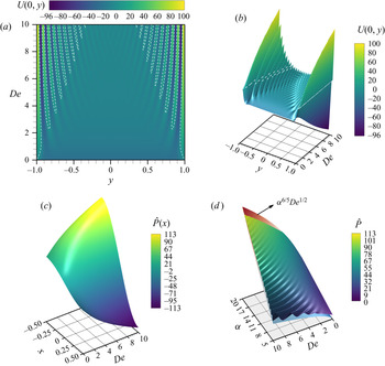
In figure 3(a) we show the level curves of velocity  $U(x=0,y)$, the real part of (2.60), projected onto the
 $y\text {--}De$ plane for
 $\alpha =20$. Here, the velocity is evaluated at the coordinate
 $x=0$, as suggested in the classical acoustic theory (Eckart Reference Eckart1948), since this is the only pressure node (
 $\hat {P}=0$), as indicated in (2.61). Figure 3 where computed at discrete values of
 $De$ from
 $y=-1$ to
 $y=1$. A fascinating outcome is shown in figures 3(a) and 3(b), where at certain values of
 $y$ and
 $De$ the velocity
 $U(x=0,y)$ acquires particularly large amplitudes. These points are known as resonance modes, useful for establishing acoustic handling of cells and particles in microfluidic systems (Bruus Reference Bruus2008). The resonant values of
 $De$ must satisfy
 $\partial U / \partial De =0$, corresponding with local maxima and/or minima of
 $U(x,y)$. From the figures mentioned above, the value of
 $\alpha =20$ makes the resonance modes located near the walls (
 $y=\pm 1$). For increasing values of
 $De$, they increase in quantity with the tendency to be located near
 $y=0$. We also observe that these resonance points arise near the zeros of the oscillatory horizontal velocity (marked with dashed white lines), where a change in sign of
 $U(0,y)$ can be seen. Therefore, to identify these zeros (
 $U(0,y)=0$) where resonance modes are in the vicinity, we note that (2.60) can be represented as a product of two complex functions
 $z_1$ and
 $z_2$, where
 $z_{j}=z(a_{j},b_{j})$,
 $a_{j}=\mathrm {Re}(z_{j})$,
 $b_{j}=\mathrm {Im}(z_{j})$ and
 $j=1,2$. We can rewrite (2.60) as
 $U(x,y)=z_{1}\boldsymbol {\cdot } z_{2}$, where
 \begin{equation} z_{1}= 1 - \frac{\cosh\left( \xi x\right) }{\cosh\left( \xi/2\right) } \end{equation}
and
 \begin{equation} z_{2}=\frac{\cosh(\zeta y)}{\cosh({\zeta })}-1. \end{equation}
It is of interest to rewrite  $z_{1}$ and
 $z_{2}$ in the form
 $z_{j}=a_{j}+{\rm i}b_{j}$. Evaluating
 $z_{1}$ at
 $x=0$, yields
 \begin{equation} z_{1}= 1 - \frac{2\cosh\left( a_{\xi}/2\right) \cos\left( b_{\xi}/2\right)}{\cosh\left( a_{\xi}\right) +\cos\left( b_{\xi}\right) }+{\rm i}\frac{2\sinh\left( a_{\xi}/2\right) \sin\left( b_{\xi}/2\right)}{\cosh\left( a_{\xi}\right)+ \cos\left( b_{\xi}\right) } \end{equation}
and  $z_{2}$ is given by
 \begin{align}
z_{2}&=\frac{\cosh[\alpha\kappa^{{1}/{2}}(y+1)]\cos[\alpha\kappa^{-{1}/{2}}(y-1)]+\cosh[\alpha\kappa^{{1}/{2}}(y-1)]
\cos[\alpha\kappa^{-{1}/{2}}(y+1)]}{\cosh[2\alpha\kappa^{{1}/{2}}]+\cos[2\alpha\kappa^{-{1}/{2}}]}
\nonumber\\ &\quad \frac{-1\sinh[\alpha\kappa^{{1}/{2}}(y\!+\!1)]\sin[\alpha\kappa^{-{1}/{2}}(y-1)]\!+\!
\sinh[\alpha\kappa^{{1}/{2}}(y-1)]\sin[\alpha\kappa^{-{1}/{2}}(y-1)]}{+ {\rm i}\,\cosh[2\alpha\kappa^{{1}/{2}}]+
\cos[2\alpha\kappa^{-{1}/{2}}]},
\end{align}
where
 \begin{equation} \kappa={-}De \pm \sqrt{De^{2} +1} \end{equation}
and
 \begin{equation} \xi=a_{\xi}+{\rm i}b_{\xi}. \end{equation}
In (4.4),  $\alpha \kappa ^{1/2}$ is the attenuation of the velocity wave, and
 $\alpha \kappa ^{-1/2}$ is the phase shift. Since the trigonometric functions in (4.4) had periods of
 $\alpha \kappa ^{-1/2}$, then the angular frequency (through increments of
 $De=\lambda _{1}\omega$) can periodically attain these values of the phase shift, creating resonance. In the following lines, what interests us is the real part of the product of
 $z_{1}\cdot z_{2}$ of (2.60), which can be expressed as
 $a_{1}a_{2}-b_{1}b_{2}$, where
 $a_{1}$ and
 $b_{1}$ are the real and imaginary parts of (4.3), respectively. The selection of the real part comes from choosing the time sine function solution of (2.31). As mentioned, the resonance points arise near the zeros of
 $U(x,y)$ with the tendency to be located near
 $y=0$, where only
 $z_{2}$ depends on the
 $y$ coordinate. Thus, from (4.4) we evaluate
 $a_{2}$ and
 $b_{2}$ at
 $y=0$ to estimate these zeros, where we found the following approximation for
 $De_{n}$ values corresponding to the number of cycles of the
 $n{\rm th}$ harmonic in the analysis interval of
 $b_{2}=0$:
 \begin{equation} De_{n}=\frac{{\rm \pi}^{4}n^4-\alpha^4}{2\alpha^2{\rm \pi}^{2}n^2}. \end{equation}
Here,  $n \in \mathbb {N^{+}}$,
 $De_{n}\geqslant 0$. Since
 $b_{2}=0$ at
 $De_{n}$, we evaluate
 $a_{1}$ at
 $De_{n}$ to figure out why
 $a_{1} a_{2}=0$. First, we numerically calculate the complex values of
 $\xi$ from (2.58). This computation shows that
 $\xi$ at
 $De_{n}$ has a small real part (
 $\gamma \ll 1$) while its imaginary part approximates
 ${\rm \pi}$
 $( \xi \rvert _{De_{n}}=\gamma +{\rm i}{\rm \pi} )$. If we rewrite (4.3) with the results of
 $\xi$, and expand using power series of
 $\gamma$, we get the following equation:
 \begin{equation} \left.z_{1}\right\vert_{De_{n}}= 1 +{\rm i} \frac{2}{\gamma}+O(\gamma). \end{equation}
From (4.8) we get  $a_{1}\neq 0$, but the product
 $z_{1}\cdot z_{2}$ still makes
 $Re[U(0,y)]=0$. This suggests that
 $z_{1}$ rotates
 $z_{2}$ by
 ${\rm \pi} /2$ in the complex plane. Therefore, we express the leading order in (4.8) in its polar form in such a manner that we can observe this rotation:
 \begin{equation} z_{1}= \frac{\sqrt{\gamma^{2}+4}}{\gamma} \exp\left[{\rm i}\phi(\gamma)\right], \end{equation}
where
 \begin{equation} \phi(\gamma) =\arctan\left(\frac{2}{\gamma}\right). \end{equation}
In the limit as  $\gamma \rightarrow 0$, (4.10) reduces to the form
 \begin{equation} \lim_{\gamma \to 0} \phi(\gamma) =\frac{\rm \pi}{2}. \end{equation}
From (4.9) and (4.11) we conclude that  $z_{1}\rvert _{De_{n}}=i$. Therefore,
 $U(0,y)$ can be expressed as
 $U(0,y)\rvert _{De_{n}}=-b_{2}+{\rm i} a_{2}$, where
 $b_{2}\rvert _{De_{n}}=0$, showing that its real part is zero.
(a) Level curves of the real part of  $U(0,y)$ at
 $x=0$ as a function of
 $y$ and
 $De$ number at
 $\alpha =20$. (b) Three-dimensional plot of the real part of
 $U(0,y)=0$ at
 $x=0$ as a function of
 $y$ and
 $De$ number at
 $\alpha =20$. (c) Three-dimensional plot of the real part of
 $\hat {P}(x)$ (from (2.61)) as a function of
 $x$ and
 $De$ number at
 $\alpha =20$. (d) Three-dimensional plot of the maximum value of the real part of
 $\hat {P}(x)$ as a function of
 $\alpha$ and
 $De$ number at
 $x=-0.5$.

With this expression for  $De_{n}$, we find that resonance modes are in the vicinity of the values obtained from (4.7). Furthermore, the number
 $n$ defines the number of resonance modes near
 $De_{n}$, e.g.
 $De_{28}=9.6$ at
 $\alpha =20$ corresponds to 28 resonance modes (see figure 3a). From this statement we observe that for increasing values of
 $De$, the resonance modes of
 $U(x,y)$ increase in quantity along the coordinate
 $y$, where
 $De_n$ depends notably on
 $\alpha$, as can be observed from (4.7). Another feature that is worth noting corresponds to the real part of the pressure
 $\hat {P}(x)$, which has local maxima and minima at these values of
 $De_{n}$ along the coordinate
 $x$; unfortunately, at
 $\alpha =20$, the
 $De_{n}$ are so close to each other that
 $\hat {P}(x)$ looks like a smooth surface, as seen in figure 3(c). This smoothness can be observed in figure 3(d), showing that with increasing values of
 $\alpha$ the acoustic pressure becomes flatter. We have found that the maximum acoustic pressure varies according to
 $\alpha ^{6/5}De^{1/2}$, as shown in figure 3(d). Equation (4.7) can be rewritten as follows:
 \begin{equation} De\left(q\right)=\frac{1}{2}\left(q^{2}-\frac{1}{q^{2}}\right), \end{equation}
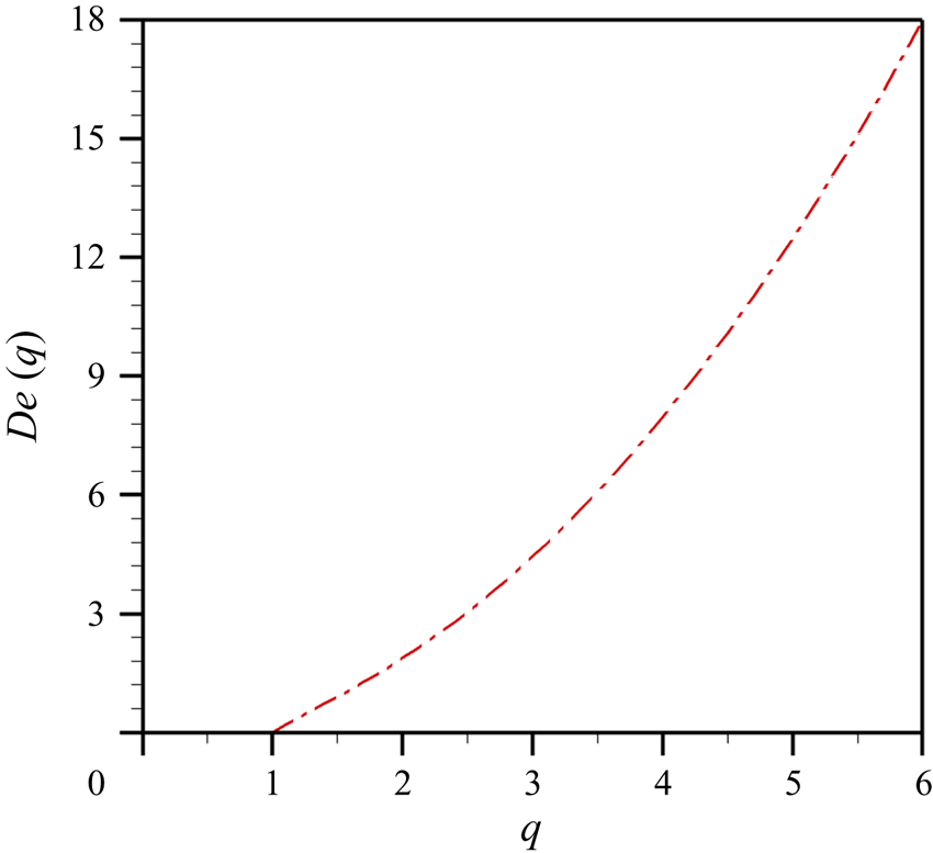
where  $q=n {\rm \pi}/\alpha$. In figure 4, we plot
 $De(q)$ versus
 $q$, which can be used in either of two forms: for a given
 $q$, the corresponding
 $De_n$ is obtained; or for a given
 $De_n$,
 $q$ is determined. For this latter case, from (4.12), we obtain
 \begin{equation} q=\sqrt{De+\sqrt{De^{2}+1}}. \end{equation}
For a fluid with a given  $De$ number, we can obtain the corresponding value of
 $q$ from (4.13), implying that we can estimate the parameter
 $\alpha$, fixing
 $n$, or vice versa; in this case, care must be taken in considering that the resonances modes
 $n$ must be a natural number. From figure 4, as a particular case, in the limit of
 $De \rightarrow 0$,
 $q=1$, meaning that
 $\alpha = n {\rm \pi}$.
 $De(q)$ evaluated at different values of
 $q$, where
 $q=n{\rm \pi} /\alpha$.

To understand the time-average stream function, (3.19), we first need to analyse the time-average vorticity function,  $\langle \varOmega _{1} \rangle$. The time-average vorticity function is shown in (3.20), where the left-hand side term is of
 $O(1)$, while the right-hand terms are of
 $O(\alpha ^{3}De^{1/2})$, neglecting terms of
 $O(\epsilon )$. From (3.20) the previous order of magnitude for the right-hand side terms is not easily observed, that is why we present how the order of magnitude for the first term appearing on the right-hand side,
 $2\alpha ^2 \langle u_0 ({\partial \varOmega _0}/{\partial x}\rangle )$, is obtained. From (2.60) we know that
 $u_0$ is
 $O(1)$. Taking the derivative with respect to
 $x$ of (3.3), and considering the leading order, we have
 ${\partial \varOmega _{0}}/{\partial x}=-{\partial ^2 u_0 }/{\partial x \partial y} + O(\epsilon ^2)$. Doing the cross derivative of (2.60) we obtain
 ${\partial ^2 u_0}/{\partial x \partial y} = \zeta \xi ({\sinh (\xi x)}/{\cosh ({\xi }/{2})}) {\sinh (\zeta y)}/{\cosh (\zeta )}$. The prefactors of this latter equation,
 $\zeta$ and
 $\xi$, are of
 $O(\alpha De^{1/2})$ and
 $O(1)$, respectively. Multiplying all factors we obtain that
 $2\alpha ^2 \langle u_0 ({\partial \varOmega _0}/{\partial x}\rangle )$ is approximately of
 $O(\alpha ^3 De ^{1/2})$. Conceptually, the first two right-hand terms are the convective derivative of Cauchy equation. The third, fourth and fifth right-hand terms come from the shear stresses of the Maxwell's model, where the third and fourth are convective terms while the fifth is related to the deformation of the material. Due to these orders of magnitudes, (
 $\alpha ^{3} De^{{1}/{2}}<\eta ^{-1}$), so that the perturbation method is valid.
In (3.19) the time-average stream function depends on two terms, the time-average vorticity and  $\langle \rho _{1} \partial u_{0}/\partial y\rangle$. Nyborg (Reference Nyborg and Mason1965) proposed using the time-average mass-transport velocity, which takes the form
 $\boldsymbol {u}^{M}=\langle \boldsymbol {u}_{1}\rangle +\langle \rho _{1}\boldsymbol {u}_{0}\rangle$, to simplify the latter term. The average mass-transport velocity relies upon the following points: (1)
 $\langle \rho _{1}\boldsymbol {u}_{0}\rangle =0$ which occur if
 $\rho _{1}$ and
 $\boldsymbol {u}_{0}$ differ in phase by
 $90^{\circ }$ (Hamilton et al. Reference Hamilton, Ilinskii and Zabolotskaya2003a), or if
 $\rho$ is aligned with the acoustic pressure
 $P$ (
 $\rho =\rho (P)$) then its nodes appear at the same time as
 $\boldsymbol {u}$ antinodes and both get cancelled; (2)
 $\langle \rho _{1} \partial u_{0}/\partial y\rangle =0$, following the same logic as point (1). Further calculations show that, due to the nature of the complex standing waves in two dimensions,
 $\langle \rho _{1} \partial u_{0}/\partial y\rangle$ do not differ in phase. Nevertheless, taking into account this term only modifies the magnitude of the streaming cells, while their size and direction stay the same even at different values of
 $\alpha$ or
 $De$. Therefore, we neglected it in the following discussion.
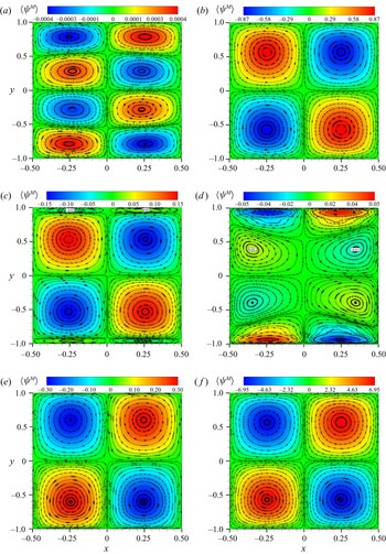
We begin this analysis with the known phenomenon that occurs in Newtonian fluids for the parameters presented in this work. Then, we observe how its behaviour is modified for the case of using a Maxwell fluid. In figures 5(a) and 5(b), the Newtonian fluid case ( $De=0$) of the time-average mass-transport is shown for different values of
 $\alpha$. Figure 5(a) shows both Stokes’ and Rayleigh's streaming cells at
 $\alpha =4.22$, while in figure 5(b), with an increase of the microchannel height (
 $\alpha =20$), the outer vortices overcome the inner streaming cells. This transition where the Rayleigh's vortices start overlapping the Stokes streaming cells in narrow channels has already been reported (Rayleigh Reference Rayleigh1884; Hamilton et al. Reference Hamilton, Ilinskii and Zabolotskaya2003a). Furthermore, four rotating streaming cells appear in the domain, which correspond to the physical lengths selected (half the wavelength along the
 $x$ axis, and
 $2H_{0}$ on the
 $y$ axis).
Acoustic streaming streamlines for the real part of the dimensionless time-average mass-transport field for (a)  $\alpha =4.22$ with
 $De=0$, and
 $\alpha =20$ with (b)
 $De=0$, (c)
 $De=1.4$, (d)
 $De=1.5$, (e)
 $De=1.7$ and (f)
 $De=5$.

For a Maxwell fluid, its behaviour is shown in figures 5(c), 5(d), 5(e) and 5(f). In figure 5(c) the resurgence of the Stokes streaming cells is visible, while the Rayleigh vortices decrease in size (in comparison with its Newtonian counterpart shown in figure 5b). With a small increment of  $De$, as shown in figure 5(d), the inner vortices dominate over the outer streaming cells, where the latter decrease in size and are pushed to the lateral walls. In figure 5(e) the reverse flow appears, where the inner streaming cells occupy the whole channel. This second transition between inner and outer vortices due to viscoelastic effects occurs in the interval
 $1< De<2$, and is induced by the fourth term on the right-hand side of (3.20) since the third and fifth terms cancel each other. That fourth term (convective term) is responsible for the growth of inner vortices and the reverse flow arises. The above assertion is based on the numeric experiments that we carried out. In figure 5(f) we observe that the magnitude of the time-average mass-transport streamlines is larger than the Newtonian case (see figure 5b), showing that elasticity can raise notably the velocity magnitude in acoustic streaming.
With this analysis we can stipulate the following. What is observed in the average mass-transport streamlines is the growth in size of the Stokes vortices and the diminishing of outer vortices due to increments of  $De$. This phenomenon is related to the attenuation of the velocity wave, as
 $De$ increases. The above can be inferred from (2.48), which can be rewritten in the following form:
 \begin{equation} \zeta =\frac{\alpha}{\sqrt{-De + \sqrt{De^{2} +1}}} \left({-}De + \sqrt{De^{2} +1}+{i}\right). \end{equation}
The above equation, (4.14), suggests that the Stokes vortices expand to the entire channel. The above can be explained from the growth of the thickness of the boundary layer ( $\delta _{\nu }$), which increases with increments of
 $De$ (Bird et al. Reference Bird, Armstrong and Hassager1987). When
 $De>1$, a second transition period, where the inner vortex dominates over the outer streaming cells, due to the convective terms of the constitutive Maxwell equation, appears. Then, the reverse flow arises when the Stokes vortices cover the whole microchannel (overlapping the Rayleigh vortices). Our hypothesis for the above sentence is that the maximum magnitude of the horizontal velocity, obtained for the Newtonian case, must be recovered for the viscoelastic fluid case at a distance from the wall equal to
 $6\delta _{\nu }/5$. In addition, while there are resonance modes for
 $De$ of
 $O(1)$ at
 $\alpha \gg 1$, they do not modify the time-average mass-transport streamlines because they are located close to the walls (see figures 3a and 3b as a reference).
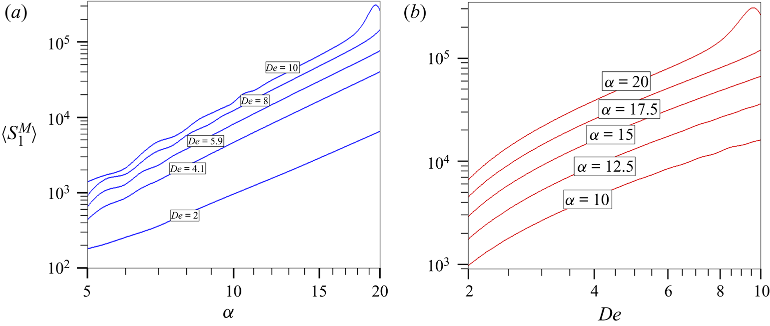
Finally, it is of interest to know the maximum value of the time-average mass-transport speed  $\langle s^{M}_{1} \rangle$ in terms of
 $\alpha$ and
 $De$. To calculate
 $\langle s^{M}_{1} \rangle$, it is necessary to evaluate the time average of the first order of (3.1a,b) as follows:
 \begin{equation} \langle s^{M}_{1} \rangle =\sqrt{\frac{\partial \langle \psi^{M}_{1}\rangle}{\partial x}^{2}+ \frac{\partial \langle \psi^{M}_{1}\rangle}{\partial y}^{2}}. \end{equation}
Through multiple numerical iterations of (4.15) the maximum value of  $\langle s_1^{M}\rangle$ is obtained, finding that
 $\langle s^{M}_{1} \rangle \sim \alpha ^{2.65}De^{1.9}$. In figures 6(a) and 6(b) the time-average mass-transport speed is shown for different values of
 $\alpha$ and
 $De$. One can observe that at high Deborah numbers the effects of the resonance modes modify
 $\langle s_1^{M}\rangle$, and when
 $\alpha \gg 1$ and
 $De>8$ the maximum magnitude of the mass-transport speed will show higher affinity for the resonance modes. In this latter case,
 $\alpha ^{2.65}De^{1.9}$ is no longer valid.
Maximum value of the time-average mass-transport speed  $\langle s^{M}_{1} \rangle$ as a function of (a)
 $\alpha$ for representative values of
 $De$ (
 $2\leqslant De \leqslant 10$), and as a function of (b)
 $De$ for representative values of
 $\alpha$ (
 $5\leqslant \alpha \leqslant 20$).

From a biological standpoint of view, blood is mainly composed of red blood cells (RBCs) and platelets, where its viscoelastic properties come from the RBCs (Qi & Shaqfeh Reference Qi and Shaqfeh2018). If blood is under a shear flow, the platelets are redistributed uniformly near the walls due to enhanced RBC mixing in the central region of the channel, where the latter migrate towards the centre due to their own deformation (Wohl & Rubinow Reference Wohl and Rubinow1974; Crowl & Fogelson Reference Crowl and Fogelson2011). As described by Antfolk & Laurell (Reference Antfolk and Laurell2019), sometimes RBCs are mixed with bacteria. In the case of medium switching, the higher acoustic impedance ( $Z_{j}\equiv \rho _{j}c_{j}$, for a material
 $j$) can induce that the bacteria end up together with the RBCs rather than staying at the side, ensuring that they would transit to the central stream. While this occurs in a Newtonian fluid, for a viscoelastic fluid, RBCs will migrate to an intermediate equilibrium position between the centreline and the wall, where the deformation and viscoelastic effects cancel each other (Chan & Leal Reference Chan and Leal1979). With the aforementioned we can compare our solutions in figure 5. If it follows increments of
 $De$, the acoustic streaming will show a transition between inner and outer vortices, where a reverse flow will appear at
 $De>1$ and the RBCs will remain at the centre. This behaviour doesn't correspond to the one obtained by Chan & Leal (Reference Chan and Leal1979), which suggests that an analysis where we consider
 $De\gg 1$ (fluid as an elastic solid) could show this behaviour.
5. Concluding remarks
Acoustic streaming in a viscoelastic fluid, which follows the Maxwell model, within a parallel flat plates microchannel has been carried out by solving the nonlinear first-order equations over a full time period. The effect of the Deborah number was analysed and several features that were not previously reported are now exhibited: we found velocity and pressure resonance points at different Deborah numbers; in acoustic streaming, the resurgence of the Stokes’ vortices and the decrease of outer streaming cells as a consequence of the convective terms of the constitutive Maxwell equation; and an increase of the velocity magnitude in acoustic streaming due to the elasticity. Finally, we show that the Deborah number has the same importance as the  $\alpha$, where the latter has created the acoustic streaming foundations, from Faraday (Reference Faraday1837) to Bruus (Reference Bruus2008).
Acknowledgements
C. Vargas thanks the Consejo Nacional de Ciencia y Tecnología (CONACYT) program for a doctoral fellowship.
Funding
The author further acknowledges financial support from the research grant no. 20210909 from Secretaría de Investigación y Posgrado del Instituto Politécnico Nacional (SIP-IPN).
Declaration of interests
The author reports no conflict of interest.
Author contributions
C. Vargas formulated the mathematical problem and obtained the corresponding semianalytical solution. All authors contributed equally to analysing data and reaching conclusions, and in writing the paper.