



1. Introduction
A sweeping jet (SWJ), a specific form of jet flow, possesses both axial momentum and lateral momentum (or angular momentum). The jet outlet demonstrates a periodic sweeping motion, which can effectively facilitate the momentum exchange between the jet and the controlled fluid. Consequently, the SWJ-based active flow control approach has drawn substantial attention in fluid mechanics (Ostermann et al. Reference Ostermann, Woszidlo, Nayeri and Paschereit2019; Wen et al. Reference Wen, Liu, Li, Peng, Zhou, Kim and Liu2020).
Currently, the active flow control approach relying on a SWJ has been successfully implemented in a wide range of scenarios. As far back as 2004, Raman & Raghu (Reference Raman and Raghu2004) initiated investigations into the applications of a SWJ in active flow control. A miniature fluidic oscillator was utilised to generate a SWJ, which effectively suppressed cavity noise by 10 dB and had a mass merely 0.12 % that of the mainstream. Subsequently, Gregory et al. (Reference Gregory, Sullivan, Raman and Raghu2007) conducted a thorough study on the characteristics of micro-fluidic oscillators in noise control. This flow control method has emerged as a prominent approach in aeroacoustic control and active flow control fields. Guyot et al. (Reference Guyot, Bobusch, Paschereit and Raghu2008) utilised a fluidic oscillator for the active control of combustion flow. Consequently, it exhibits a longer service life and greater reliability. This makes it highly appropriate for applications in industrial gas turbines, as it does not contain any moving components or complex structures. Seele et al. (Reference Seele, Tewes, Woszidlo, McVeigh, Lucas and Wygnanski2009) incorporated a fluidic oscillator onto the V-22 aerofoil to manage flow separation. The findings demonstrated that under suitable control conditions, the lift-to-drag ratio of the wing could be notably enhanced. Subsequently, experiments were carried out on the V-22 wing/nacelle combination. The results revealed that upon implementing active flow control, the lift-to-drag ratio increased by approximately 60 %. Woszidlo et al. (Reference Woszidlo, Nawroth, Raghu and Wygnanski2010) further validated, via experimental research, the efficacy of the SWJ array in suppressing the flow separation of multiple flaps. National Aeronautics and Space Administration (NASA) (Seele et al. Reference Seele, Graff, Gharib, Taubert, Lin and Wygnanski2012; Whalen et al. Reference Whalen, Shmilovich, Spoor, Tran, Vijgen, Lin and Andino2018; Andino et al. Reference Andino, Lin, Roman, Graff, Gharib, Whalen and Wygnanski2019; Lin et al. Reference Lin, Whalen, Andino, Graff, Lacy, Washburn, Gharib and Wygnanski2019) carried out in-depth research on the application of fluidic oscillators in the vertical tail wings of a Boeing-757 commercial transports aircraft. The findings from wind tunnel experiments and flight tests indicated that the SWJ effectively suppressed the flow separation of the rudder and significantly enhanced the control capacity of the rudder. The implementation of this technology has the potential to reduce the area of the vertical tail by 17 %, leading to a 0.5 % reduction in the total drag of the entire aircraft.
The application of SWJs on the vertical tail of the Boeing-757 demonstrated their potential for active flow control and triggered extensive research on their use in engineering flows. Park et al. (Reference Park, Kara and Kim2018) applied a SWJ to impact cooling of a flat plate. The results showed that the SWJ could cover a wide area and had a stronger average heat transfer performance compared with the steady jet. Chen & Li (Reference Chen and Li2022) used a SWJ to control the tip leakage flow of the turbine cascade in an aircraft engine, reducing the total pressure loss by 20.1 %. Lee et al. (Reference Lee, Roh and Lee2023) employed an SWJ to inject hydrogen into the supersonic flow, achieving the mixing of fuel and air within a hypersonic scramjet engine. Fan et al. (Reference Fan, Zhang, Xiang and Feng2024) implemented the SWJ active flow control method for hypersonic reactive flow within the combustion chamber of the oblique detonation engine. The findings indicated that the SWJ not only had the ability to regulate the wave structure but also could enhance the turbulence intensity of the main flow. Consequently, this improvement led to the enhancement of the initiation and combustion stability of the oblique detonation wave. Wang et al. (Reference Wang, Shi, Li, He, Zhou, Wen and Liu2025) used a SWJ to create an air film for the cooling of high-pressure guide vanes, which led to a 42 % enhancement in cooling efficiency.
In the field of numerical simulation of a SWJ, research has progressed from early two-dimensional simulations to three-dimensional approaches (Gokoglu et al. Reference Gokoglu, Kuczmarski, Culley and Raghu2011; Aram et al. Reference Aram, Lee, Shan and Vargas2018), with computational methods advancing from unsteady Reynolds-averaged Navier–Stokes (URANS) to hybrid RANS–large eddy simulation (LES) and even to LES (Aram & DeJong Reference Aram and DeJong2018; Hossain et al. Reference Hossain, Prenter, Lundgreen, Ameri, Gregory and Bons2018). The lattice Boltzmann method (LBM) offers advantages such as robust numerical stability, low dissipation, high computational efficiency and the ability to effortlessly handle complex flow channels (Feng et al. Reference Feng, Guo, Jacob and Sagaut2019b ). By integrating the LBM with LES, this approach achieves high computational efficiency while maintaining excellent accuracy in turbulence solving, thereby offering a suitable method for simulating the complex flow dynamics of the SWJ. Duda et al. (Reference Duda, Fares, Wessels and Vatsa2016) employed the LBM–VLES (very large eddy simulation) method to simulate the internal and external flows in a fluidic oscillator. Their results showed that the simulated transient pressure and frequency spectrum were in quantitative agreement with experimental data; however, the numerical predictions for both the mean and fluctuating quantities at the outlet were overestimated. In a numerical study of the fluidic oscillator using the multiple-relaxation-time LBM method, Mohammed (Reference Mohammed2020) found that within the jet Reynolds number range from 180 to 300, the oscillation amplitude and frequency increased linearly with Reynolds number. Fan et al. (Reference Fan, Wang and Feng2025) applied the regularised LBM–LES approach with subgrid-scale (SGS) models including Smagorinsky, Vreman and wall-adapting local eddy-viscosity (WALE) to simulate both a free SWJ and a SWJ with wall interference. Their results indicated that all three models provided quantitatively good agreement with experimental measurements in predicting both time-resolved and time-averaged characteristics. Furthermore, the LBM method has also been applied to simulations of plasma jets (Zhang et al. Reference Zhang, Hu, Wang and Zhu2007), isothermal and non-isothermal jet flow fields and acoustic fields (Noah et al. Reference Noah, Lien and Yee2021), as well as thermal impinging jet flows (Nguyen et al. Reference Nguyen, Boussuge, Sagaut and Larroya-Huguet2022), among other areas.
To apply the active flow control approach based on a SWJ more effectively to certain special scenarios, investigating the interaction between the SWJ and the main flow holds significant practical value. Consequently, from the perspective of practical applications, researchers have conducted investigations on the interaction characteristics between the SWJ and the controlled main flow. Oshima et al. (Reference Oshima, Wygnanski and Gharib2022) conducted a study on the interaction between the wing leading-edge vortex and the SWJ. The findings indicated that the lift-enhancing capabilities of the SWJ are closely associated with the intensity of the vortex lift. Recently, Chen et al. (Reference Chen, Zhong, Liu, Ozer and Gao2024) carried out an experimental investigation into the interaction between a SWJ and the afterbody vortices of high-speed trains. Their findings revealed that when the velocity ratio of the main flow to the SWJ was 6.4, the kinetic energy of the SWJ was injected into the core of the tail vortex. Consequently, this led to a reduction of 17.7 % in the total velocity and 15.9 % in the horizontal slip flow.
Research aimed at practical applications of SWJs has long been limited by the difficulty of extracting general physical principles that govern the interaction between a SWJ and an external crossflow. Motivated by this challenge, several studies have explored the canonical configuration of a SWJ issuing into a plate crossflow. Using time-resolved stereoscopic particle image velocimetry under incompressible conditions, Ostermann et al. (Reference Ostermann, Woszidlo, Nayeri and Paschereit2016) demonstrated that the counter-rotating vortex pair (CVP), largely governed by the SWJ dynamics, dominates the streamwise flow structure. Later work identified the jet-to-crossflow velocity ratio (or its equivalent Strouhal number) as the sole governing parameter characterising the resulting flow field (Ostermann et al. Reference Ostermann, Woszidlo, Nayeri and Paschereit2019). Moreover, once this ratio exceeds approximately five, the SWJ-induced perturbation approaches a quasi-steady regime (Ostermann et al. Reference Ostermann, Woszidlo, Nayeri and Paschereit2017). Experimental observations and complementary numerical simulations by Aram & DeJong (Reference Aram and DeJong2018) and Aram & Shan (Reference Aram and Shan2019) further indicate that the rapid decay of the SWJ outlet velocity leads to a significantly shallower penetration compared with that of a steady jet. At the same time, SWJs inject substantially higher turbulent kinetic energy into the downstream flow, endowing them with superior mixing performance relative to steady jets. The skew angle of the jet exit has also been shown to strongly influence jet–crossflow interaction. In particular, Ostermann et al. (Reference Ostermann, Woszidlo, Nayeri and Paschereit2020) reported that decreasing the skew angle enhances wall-normal penetration, which, at a skew angle of 0
 $^\circ$
, becomes comparable to that of a steady jet.
Despite these advances, the SWJs used in the above studies were invariably generated using fixed fluidic oscillator geometries, which couple the outlet velocity and oscillation frequency through a strong device-specific relationship. For instance, in double-feedback fluidic oscillators under incompressible conditions, these two quantities vary approximately linearly. Consequently, the independent influence of oscillation frequency on the flow cannot be isolated, as identical outlet velocities cannot be achieved across different frequencies using a single fluidic oscillator design. This limitation hinders the systematic exploration of how temporal and spatial characteristics of SWJs affect the controlled crossflow.
Motivated by these challenges, we employ the LBM-based LES (LBM–LES), which is highly attractive for its simplicity, computational efficiency and ability to accurately resolve the fine, unsteady features inherent to both SWJs and crossflows. In this work, the SWJ is generated numerically through an unsteady phenomenological model, allowing the jet characteristics to be prescribed arbitrarily and independently of fluidic oscillator geometry. With the LBM–LES solver carefully calibrated and validated, we apply it to systematically examine how spatial variations (including the SWJ opening angle and skew angle) and temporal variations (controlled through the oscillation frequency) influence the SWJ–crossflow interaction. This framework provides a controlled setting in which the isolated effects of fundamental SWJ parameters can be rigorously assessed, addressing key limitations of previous experimental and numerical studies.
The paper is structured as follows. Section 2 presents the numerical methodology, including the LBM-LES, and the phenomenological model used to generate the SWJ. Section 3 describes the computational set-up, detailing the domain configuration, grid resolution, boundary conditions and the validation procedure. Section 4 provides the results and discussion, where the effects of the SWJ characteristics on the jet–crossflow interaction are systematically examined. Finally, § 5 summarises the key findings and offers concluding remarks.
2. Numerical methodology
In this study, an LES method within the LBM framework is employed to efficiently and accurately simulate the rich and intricate vortex structures generated by the interaction between the SWJ and the crossflow.
2.1. Large eddy simulation
Existing research has shown that the transient vortex structures generated at the outlet of the SWJ are not adequately captured within the URANS framework (Aram et al. Reference Aram, Lee, Shan and Vargas2018). Thus, the use of the more accurate LES approach is considered necessary. In LES, it is first necessary to distinguish between the large-scale and small-scale components of the flow field. This study primarily focuses on low-speed flows (Mach numbers less than 0.3), and the adopted filter scale is consistent with the grid scale. The filtered incompressible Navier–Stokes equations are (Sagaut Reference Sagaut2005)
 \begin{equation} {\frac {{\partial {{\bar u}_{\kern-0.5pt i}}}}{{\partial {x_i}}} = 0} ,\end{equation}
 \begin{equation} {\frac {{\partial {{\bar u}_{\kern-0.5pt i}}}}{{\partial t}}+ \frac {{\partial {{\bar u}_{\kern-0.5pt i}}{{\bar u}_{\!j}}}}{{\partial {x_{\!j}}}}= - \frac {1}{ \rho }\frac {{\partial \bar p}}{{\partial {x_i}}} + \nu \frac {{{\partial ^2}{{\bar u}_{\kern-0.5pt i}}}}{{\partial {x_{\!j}}^2}} - \frac {{\partial \tau _{\textit{ij}}^{\textit{SGS}}}}{{\partial {x_{\!j}}}}}, \end{equation}
where
 ${\bar u}_i$
are filtered flow velocities (
 $i$
= 1, 2, 3 correspond to the three spatial directions, respectively),
 $x_i$
is spatial locations,
 $t$
is time,
 $ \rho$
is the fluid density,
 $\bar p$
is the filtered pressure,
 $\nu$
is the kinematic viscosity.
The SGS stress
 $\tau _{\textit{ij}}^{\textit{SGS}}$
, in (2.2), characterises the influence of small-scale eddies on large-scale motion. The expression is given as, based on the eddy viscosity hypothesis (Sagaut Reference Sagaut2005),
 \begin{equation} \tau _{\textit{ij}}^{\textit{SGS}} = -2 \nu _{\textit{SGS}} \bar S_{\textit{ij}} + \frac {1}{3} \tau _{\textit{kk}}^{\textit{SGS}} \delta _{\textit{ij}} ,\end{equation}
where
 $ \nu _{\textit{SGS}}$
represents the eddy viscosity and
 $ \bar S_{\textit{ij}}$
is the filtered strain rate tensor:
 \begin{equation} {\bar S_{\textit{ij}}} = \frac {1}{2}\left ( {\frac {{\partial {{\bar u}_{\kern-0.5pt i}}}}{{\partial {x_{\!j}}}} + \frac {{\partial {{\bar u}_{\!j}}}}{{\partial {x_i}}}} \right ) .\end{equation}
The SGS effects are modelled in this study using the Smagorinsky model (Smagorinsky Reference Smagorinsky1963). In the current LBM–LES approach, the effective viscosity is calculated as (Sagaut Reference Sagaut2010; Malaspinas & Sagaut Reference Malaspinas and Sagaut2012)
 \begin{equation} \nu _{\textit{eff}} = \nu + \nu _{\textit{SGS}} = \nu + {\left ( {{C_s}\Delta } \right )^2}\left | {\bar S} \right | ,\end{equation}
where the Smagorinsky constant
 $ C_s$
, typically in the range of 0.1–0.2, is adopted as 0.15 in this study and
 $ \Delta$
represents the filter width, which is related to the grid scale, the modulus of the strain rate tensor is calculated as
 \begin{equation} \left | {\bar S} \right | = \sqrt {2{{\bar S}_{\textit{ij}}}{{\bar S}_{\textit{ij}}}} .\end{equation}
2.2. Lattice Boltzmann framework
The above governing equations of LES are solved by recursive regularised LBM in this work. The LBM simulations employ the D3Q19 lattice configuration. The evolution of the distribution function
 $f_\alpha$
follows (Qian et al. Reference Qian, d’Humières and Lallemand1992; Succi Reference Succi2001)
 \begin{equation} {f_\alpha }\left ( {{x_i} + {c_{\alpha ,}}_i\Delta t,t + \Delta t} \right ) = f_\alpha ^{eq}\left ( {{x_i},t} \right ) + \left ( {1 - \frac {1}{\tau }} \right )f_\alpha ^{neq}\left ( {{x_i},t} \right ) ,\end{equation}
where
 $f_\alpha ^{eq}$
and
 $f_\alpha ^{neq}$
represent the equilibrium and non-equilibrium distribution functions, respectively. The relationship between the two functions is defined by the equation
 $f_\alpha ^{neq}$
=
 $f_\alpha$
–
 $f_\alpha ^{eq}$
. The left-hand side of (2.7) indicates that at time
 $t$
, the fluid particles located at position
 $x_i$
undergo a migration on the lattice in the discrete velocity direction
 $c_{\alpha ,i}$
after a lattice time step
 $\Delta t$
. The right-hand side characterises the collision effect during the process in which particles approach equilibrium from a non-equilibrium state. Among them, the relaxation time
 $\tau$
is used to control the kinematic viscosity
 $\nu$
on the lattice (Succi Reference Succi2001), i.e.
 \begin{equation} \nu = c_s^2\left ( {\tau - \frac {\Delta t}{2}} \right ), \end{equation}
where
 $c_s$
is the speed of sound. The macroscopic density and momentum can be updated through the calculation of the moments of the particle distribution function. The macroscopic quantity of D3Q19 is calculated in the following manner:
 \begin{equation} \begin{array}{l} \rho = \sum \limits _{\alpha = 0}^{18} {{f_\alpha }} ,\\ \rho {u_{\kern-0.5pt i}} = \sum \limits _{\alpha = 0}^{18} {{c_{\alpha ,i}}{f_\alpha }} .\end{array} \end{equation}
To address the numerical instability of traditional LBM in high-Reynolds-number flows, Latt & Chopard (Reference Latt and Chopard2006) introduced the regularised LBM. By reconstructing the non-equilibrium distribution function, it is possible retaining the lower-order moments related to macroscopic conservation laws while filtering out higher-order moment information. As a result, the method effectively suppresses numerical noise, thereby enhancing numerical stability. Building upon this framework, Jacob et al. (Reference Jacob, Malaspinas and Sagaut2018) subsequently proposed the hybrid recursive regularisation (HRR) model, which further improves the regularisation process through a more sophisticated treatment of moment evolution. The present study will employ this HRR model.
The local equilibrium distribution function can be expressed as (Dellar Reference Dellar2014; Jacob et al. Reference Jacob, Malaspinas and Sagaut2018; Feng et al. Reference Feng, Guo, Jacob and Sagaut2021b )
 \begin{equation} \begin{array}{l} f_\alpha ^{eq} = {w_\alpha }\left \{ {\rho + \frac {{{c_{a,i}}\rho {u_{\kern-0.5pt i}}}}{{c_s^2}} + \frac {{{{\mathcal H}_{\alpha ,\textit{ij}}}{\mathcal A}_{\textit{ij}}^{\left ( 0 \right )}}}{{2c_s^4}} + \frac {1}{{6c_s^6}}} \right .\\[4pt] \quad\left [ {3\left ( {{{\mathcal H}_{\alpha ,xxy}} + {{\mathcal H}_{\alpha ,yzz}}} \right )\left ( {{\mathcal A}_{xxy}^{\left ( 0 \right )} + {\mathcal A}_{yzz}^{\left ( 0 \right )}} \right ) + \left ( {{{\mathcal H}_{\alpha ,xxy}} - {{\mathcal H}_{\alpha ,yzz}}} \right )\left ( {{\mathcal A}_{xxy}^{\left ( 0 \right )} - {\mathcal A}_{yzz}^{\left ( 0 \right )}} \right )} \right .\\[4pt] \quad+\, 3\left ( {{{\mathcal H}_{\alpha ,xzz}} + {{\mathcal H}_{\alpha ,xyy}}} \right )\left ( {{\mathcal A}_{xzz}^{\left ( 0 \right )} + {\mathcal A}_{xyy}^{\left ( 0 \right )}} \right ) + \left ( {{{\mathcal H}_{\alpha ,xzz}} - {{\mathcal H}_{\alpha ,xyy}}} \right )\left ( {{\mathcal A}_{xzz}^{\left ( 0 \right )} - {\mathcal A}_{xyy}^{\left ( 0 \right )}} \right )\\[4pt] \quad\left . {\left . { +\, 3\left ( {{{\mathcal H}_{\alpha ,yyz}} + {{\mathcal H}_{\alpha ,xxz}}} \right )\left ( {{\mathcal A}_{yyz}^{\left ( 0 \right )} + {\mathcal A}_{xxz}^{\left ( 0 \right )}} \right ) + \left ( {{{\mathcal H}_{\alpha ,yyz}} - {{\mathcal H}_{\alpha ,xxz}}} \right )\left ( {{\mathcal A}_{yyz}^{\left ( 0 \right )} - {\mathcal A}_{xxz}^{\left ( 0 \right )}} \right )} \right ]} \right \}\!,\end{array} \end{equation}
where
 $w_\alpha$
is the weight of discrete equilibrium distribution function. Here
 ${{\mathcal H}_{\alpha ,\textit{ij}}} = {c_{\alpha ,i}}{c_{\alpha ,j}} - c_s^2{\delta _{\textit{ij}}}$
,
 $ {{\mathcal H}_{\alpha ,\textit{ij}k}} = {c_{\alpha ,i}}{c_{\alpha ,j}}{c_{\alpha ,k}} - c_s^2{ [ {{c_\alpha }\delta } ]_{\textit{ijk}}}$
are second-order and third-order Hermite polynomials with
 $\delta _{\textit{ij}}$
and
 $ [ {{c_\alpha }\delta } ]_{\textit{ijk}}$
being classic Kronecker matrices. The discrete velocities and the corresponding weights on the D3Q19 lattice are presented as follows:
 \begin{equation} \left [ {{c_{\alpha ,i}},{w_\alpha }} \right ] = \left \{ {\begin{array}{*{20}{c}} {\left [ {\left ( {0,0,0} \right ),1/3} \right ]},\\ {\left [ {\left ( { \pm 1,0,0} \right ),\left ( {0, \pm 1,0} \right ),\left ( {0,0, \pm 1} \right ),1/18} \right ]},\\ {\left [ {\left ( { \pm 1, \pm 1,0} \right ),\left ( { \pm 1,0, \pm 1} \right ),\left ( {0, \pm 1, \pm 1} \right ),1/36} \right ],{\textrm { }}} \end{array}\begin{array}{*{20}{c}} {\alpha {\textrm {=}}0},\\ {\alpha {\textrm {=}}1\sim 6},\\ {\alpha {\textrm {=}}7\sim 18}. \end{array}} \right . \end{equation}
The non-equilibrium distribution function can also be expanded in the Hermite polynomial basis as
 \begin{equation} \begin{array}{l} f_\alpha ^{neq} = {w_\alpha }\left \{ { \frac {{{{\mathcal H}_{\alpha ,\textit{ij}}}{\mathcal A}_{\textit{ij}}^{\left ( 1 \right )}}}{{2c_s^4}} + \frac {1}{{6c_s^6}}} \right .\\ \quad\left [ {3\left ( {{{\mathcal H}_{\alpha ,xxy}} + {{\mathcal H}_{\alpha ,yzz}}} \right )\left ( {{\mathcal A}_{xxy}^{\left ( 1 \right )} + {\mathcal A}_{yzz}^{\left ( 1 \right )}} \right ) + \left ( {{{\mathcal H}_{\alpha ,xxy}} - {{\mathcal H}_{\alpha ,yzz}}} \right )\left ( {{\mathcal A}_{xxy}^{\left ( 1 \right )} - {\mathcal A}_{yzz}^{\left ( 1 \right )}} \right )} \right .\\[4pt] \quad+\, 3\left ( {{{\mathcal H}_{\alpha ,xzz}} + {{\mathcal H}_{\alpha ,xyy}}} \right )\left ( {{\mathcal A}_{xzz}^{\left ( 1 \right )} + {\mathcal A}_{xyy}^{\left ( 1 \right )}} \right ) + \left ( {{{\mathcal H}_{\alpha ,xzz}} - {{\mathcal H}_{\alpha ,xyy}}} \right )\left ( {{\mathcal A}_{xzz}^{\left ( 1 \right )} - {\mathcal A}_{xyy}^{\left ( 1 \right )}} \right )\\[4pt] \quad\left . {\left . { +\, 3\left ( {{{\mathcal H}_{\alpha ,yyz}} + {{\mathcal H}_{\alpha ,xxz}}} \right )\left ( {{\mathcal A}_{yyz}^{\left ( 1 \right )} + {\mathcal A}_{xxz}^{\left ( 1 \right )}} \right ) + \left ( {{{\mathcal H}_{\alpha ,yyz}} - {{\mathcal H}_{\alpha ,xxz}}} \right )\left ( {{\mathcal A}_{yyz}^{\left ( 1 \right )} - {\mathcal A}_{xxz}^{\left ( 1 \right )}} \right )} \right ]} \right \}\!,\end{array} \end{equation}
where
 ${\mathcal A}_{\textit{ij}}^{ ( 1 )}$
is the second-order non-equilibrium moment and
 ${\mathcal A}_{\textit{ijk}}^{ ( 1 )}$
is the third-order non-equilibrium moment.
Owing to the Chapman–Enskog technique, the projection of the non-equilibrium distribution function onto the Hermite polynomial basis and its finite difference (FD) approximation can be expressed as follows (Feng et al. Reference Feng, Boivin, Jacob and Sagaut2019a ):
 \begin{align} {\mathcal A}_{\textit{ij}}^{\left ( {1} \right )} &= \sum \limits _i {{c_{\alpha ,i}}} {c_{\alpha ,j}}f_\alpha ^{neq},\nonumber\\ {\mathcal A}_{\textit{ij}}^{\left ( {1,FD} \right )} &\approx - \Delta t\overline \tau \rho c_s^2\left ( {\frac {{\partial {u_j}}}{{\partial {x_i}}} + \frac {{\partial {u_i}}}{{\partial {x_{\!j}}}} - \frac {2}{3}\frac {{\partial {u_k}}}{{\partial {x_k}}}{\delta _{\textit{ij}}}} \right )\!.\end{align}
Then the hybrid regularised second-order non-equilibrium moment can be alternatively reconstructed relying on the linear combination of the
 ${\mathcal A}_{\textit{ij}}^{ ( {1} )}$
and
 ${\mathcal A}_{\textit{ij}}^{ ( {1,FD} )}$
. Furthermore, the third-order term is recursively updated. In the HRR collision model the following non-equilibrium moments are used in (2.12):
 \begin{align} {\mathcal A}_{\textit{ij}}^{\left ( {1,HRR} \right )} & = \sigma {\mathcal A}_{\textit{ij}}^{\left ( {1} \right )} + \left ( {1 - \sigma } \right ){\mathcal A}_{\textit{ij}}^{\left ( {1,FD} \right )}, \end{align}
 \begin{align} {\mathcal A}_{\textit{ijk}}^{\left ( {1,HRR} \right )} &= {u_i}{\mathcal A}_{jk}^{\left ( {1,HRR} \right )} + {u_j}{\mathcal A}_{ik}^{\left ( {1,HRR} \right )} + {u_k}{\mathcal A}_{\textit{ij}}^{\left ( {1,HRR} \right )}. \end{align}
Here
 $\sigma \in [ {0,1} ]$
represents the mixed weight coefficient. In the present work, for the sake of simplicity and efficiency, we adopt a constant value of 0.99, which is a commonly used and well-validated choice in Feng et al. (Reference Feng, Boivin, Jacob and Sagaut2021a
) and Jacob & Sagaut (Reference Jacob and Sagaut2018). The discretisation error introduced by the FD component effectively acts as a form of high-order artificial viscosity, which contributes to the robustness of the LBM, as well as an implicit LES.
2.3. The SWJ phenomenological model
Numerical simulations of fluidic oscillators are often hampered by high computational expense and prolonged simulation times. First, the intricate internal geometry and complex flow physics necessitate a large computational mesh. Second, a significant duration is required for the fluid medium to establish a stable SWJ at the outlet; computations during this phase contribute minimally to flow control studies and largely constitute a waste of computational resources. Third, the design of flow control applications often necessitates repeated simulations of internal flows within fluidic oscillators, substantially increasing both the development time and cost associated with control strategy design.
Therefore, this study utilises an unsteady phenomenological mathematical model to describe a SWJ. By implementing this model as an unsteady boundary condition at the jet outlet, a SWJ suitable for flow control applications is produced. Furthermore, the characteristic parameters of the jet within the model can be flexibly adjusted according to specific requirements. Notably, the SWJ employed in this work is not limited to those generated by any particular class of fluidic oscillator (e.g. feedback-free fluidic oscillator, single-feedback loop fluidic oscillator, double-feedback channel fluidic oscillator, etc.).
The fundamental concept underlying the model is to provide both the instantaneous magnitude and the direction of the SWJ velocity at the boundary. The outlet velocity magnitude
 $U_{\textit{bulk}}$
does not change with time, and the jet direction is determined by establishing the variation of the jet deflection angle
 $\theta$
with time. The specific functional relationship is as follows:
 \begin{equation} \theta \left ( \bar {t} \right ) = \theta _{max} \boldsymbol{\cdot }{\textrm {sign}}\left ( {\sin \bar {t}} \right ) \boldsymbol{\cdot }{\left ( {{\textrm {abs}}\left ( {\sin \bar {t}} \right )} \right )^k} .\end{equation}
Here
 $\theta _{max}$
represents the maximum jet deflection angle and
 $k$
is the adjustment factor, with a range of (0, 1]. Following meticulous calculation and calibration, adopting a constant value of 0.7 can effectively mimic the SWJ produced by the double-feedback fluidic oscillator.
In (2.16) the sign and abs symbols denote a symbolic function and an absolute value function, respectively. Here
 $\bar {t}$
is the normalised time and its expression is
 \begin{equation} \bar {t} = 2\pi \boldsymbol{\cdot }\left ( {t - [ {t/T} ] \boldsymbol{\cdot }T} \right )/T ,\end{equation}
where
 $t$
represents physical time and
 $T$
is the oscillation period. The square brackets indicate rounding down to the nearest integer that is not greater than the number within the brackets.
The angle between the oscillation plane and the positive
 $x$
axis is
 $\beta$
(see figure 1
b). The velocities in three directions with respect to time are
 \begin{equation} \begin{array}{l} {u_1} = {U_{\textit{bulk}}} \boldsymbol{\cdot }\sin \theta \cos \beta, \\ {u_2} = {U_{\textit{bulk}}} \boldsymbol{\cdot }\cos \theta ,\\ {u_3} = {U_{\textit{bulk}}} \boldsymbol{\cdot }\sin \theta \sin \beta ,\end{array} \end{equation}
where
 $\beta$
is the skew angle. The subscripts 1, 2 and 3 correspond to the
 $x$
,
 $y$
and
 $z$
directions, respectively, as labelled in figure 1(b). When
 $\beta$
= 90
 $^\circ$
, the oscillation plane is perpendicular to the direction of the crossflow.
3. Computational set-up
3.1. Physical model and domain
The fundamental flow scenario of a SWJ injection into a uniform crossflow is taken into account. The working medium for both the jet and the crossflow is air. According to Aram & Shan (Reference Aram and Shan2019), the fluidic oscillator is embedded and installed beneath the desktop. A Cartesian coordinate system is established with the centre point of the outlet throat as the origin, as depicted in figure 1(a). The hydraulic diameter
 $d_h$
of the square throat at the outlet of the SWJ is 10 mm. The range of the computational domain in the
 $x$
direction is from −50
 $d_h$
to 150
 $d_h$
, in the
 $y$
direction from 0
 $d_h$
to 37
 $d_h$
and in the
 $z$
direction from −50
 $d_h$
to 50
 $d_h$
.
Schematic of (a) the interaction between the SWJ and the crossflow, (b) the geometric relationship of the SWJ opening angle and skew angle, (c) the computational domain dispersed by a Cartesian grid and the boundary conditions.

Figure 1. Long description
Panel A: A three-dimensional diagram showing the interaction between a sweeping jet and crossflow. The fluidic oscillator generates a sweeping jet that interacts with the crossflow near a wall. The axes are labeled as x, y, and z. Panel B: A diagram depicting the geometric relationship of the sweeping jet opening angle (β) and skew angle (ψ). The angles are shown in relation to the x, y, and z axes. Panel C: A three-dimensional diagram of the computational domain dispersed by a Cartesian grid. The domain is divided into different regions labeled as slide wall, SWJ model, wall model, velocity inlet, and far field. The dimensions of these regions are provided in terms of d_h units.
Figure 1(b) illustrates the geometric relationship of the opening angle
 $\psi$
and the skew angle
 $\beta$
of the SWJ. The maximum jet deflection angle of the SWJ is
 $\pm$
45
 $^\circ$
. The Strouhal number, representing the frequency characteristic, is defined as
 \begin{equation} St = \frac {{{f_{\textit{OSC}}} \boldsymbol{\cdot }{d_h}}}{{{U_{\textit{bulk}}}}} ,\end{equation}
where
 $f_{\textit{OSC}}$
is the oscillation frequency and
 $U_{\textit{bulk}}$
is the average velocity magnitude of the SWJ at the outlet. Based on the experimental conditions,
 $U_{\textit{bulk}}$
is 45 m s−1 and the oscillation frequency is 67 Hz. Thus, the value of
 $St$
is 0.015 in this scenario.
The velocity ratio of the SWJ to crossflow is defined as
 \begin{equation} R = \frac {{{U_{\textit{bulk}}}}}{{{U_{\textit{in}} }}} ,\end{equation}
where
 $U_{\textit{in}}$
is the velocity of the crossflow. Based on previous research, the velocity ratio stands as the only parameter influencing the trajectory of the jet. The greater its value, the deeper the penetration depth of the SWJ within the crossflow and the more intricate the interference characteristics between the jet and the crossflow become (Ostermann et al. Reference Ostermann, Woszidlo, Nayeri and Paschereit2019). This complex flow field structure can effectively test the capacity of numerical simulation methods in capturing fine vortex structures. Hence, in this study the case with a velocity ratio of 3 is chosen for numerical simulation, namely,
 $U_{\textit{in}}$
= 15 m s−1.
3.2. Boundary condition and grid
As shown in figure 1(c), the crossflow and SWJ are set to velocity inlet boundaries. This study adopts the non-equilibrium reconstruction method (Feng et al. Reference Feng, Boivin, Jacob and Sagaut2021a
). The
 $\rho$
and
 $u_i$
are set as Dirichlet boundary conditions at the boundary grid points. The distribution function on the non-boundary grid points of the first layer is constructed using the following relationship:
 \begin{equation} {f_\alpha } = f_\alpha ^{eq}\left ( {\rho ,{u_i}} \right ) + f_\alpha ^{neq}\left ( {{\mathcal A}_{\textit{ij}}^{\left ( 1 \right )},{\mathcal A}_{\textit{ijk}}^{\left ( 1 \right )}} \right ). \end{equation}
The density of non-boundary grid points in the first layer is computed based on adjacent grid points.
The bottom surface of the computational domain is defined as a wall boundary. The wall boundary layer effect represents a crucial characteristic of the crossflow over a flat plate. Precisely calculating the thickness of the boundary layer serves as a prerequisite for accurately capturing the interaction between the wall-impinging SWJ and the crossflow. It is essential to account for the turbulent effect near the wall by employing a wall model. This study employs the classical logarithmic law model,
 \begin{equation} {u^ + } = \frac {u}{{{u_\tau }}} = \frac {1}{\kappa }\ln {y^ + } + B ,\end{equation}
where
 $\kappa$
is the von Kármán constant, with a value of 0.41,
 $B$
is a constant under a smooth wall surface, with a value of 5.0, and
 $u_\tau$
is the wall friction velocity.
The top surface is configured as a slip wall. The SWJ outlet is positioned at the origin and the boundary conditions of the SWJ phenomenological model are imposed. The model input parameters are summarised in table 1. All remaining surfaces are designated as far fields. At the far-field boundary, the density is prescribed as the environment density using a Dirichlet boundary condition.
The input parameters of the SWJ phenomenological model under all conditions.

Table 1. Long description
Panel A: Table. The table has two columns labeled ‘Parameters’ and ‘Values’. The ‘Parameters’ column lists Ubulk, Theta max, k, Beta, and Fosc. The ‘Values’ column lists 45 m s^-1, 45 degrees, 0.7, 0 degrees, 45 degrees, 90 degrees, and 34 Hz, 67 Hz, 134 Hz respectively.
The four-layer locally refined Cartesian grid is adopted for the calculation, as depicted in figure 1(c). The total number of grid cells is approximately 20 million. The minimum spatial step size of this grid is set at 0.000625 m. Consequently, the square outlet of the SWJ comprises a
 $16\times 16$
grid array. The time-step size
 $\delta t$
is computed in accordance with the spatial step size to satisfy the stability criterion of the LBM. Specifically, the minimum time step is
 $1.23\times 10^{-6}$
s. It should be noted that all results – including the validation examples and the research conditions described subsequently – are obtained using the same grid and time step.
This paper primarily investigates the interaction flow field using time-averaged flow data. Once the flow field has reached a statistically steady state, starting from the specified initial time step, the transient physical quantities (e.g. velocity, density) at each grid node are accumulated over successive time steps throughout the simulation. Upon completion of the prescribed statistical duration, the time-averaged values of these quantities are computed by dividing the accumulated sums by the total number of time steps included in the averaging window. In this study, a time interval corresponding to 20 oscillation cycles is adopted for time averaging. This duration has been validated to be sufficiently long to capture the fully developed time-averaged flow characteristics.
Some of the results presented herein pertain to the phase-averaged flow field; therefore, details of the phase-averaging procedure are provided. One oscillation cycle of the SWJ is discretised into 360 equally spaced phase intervals, each corresponding to a 1
 $^\circ$
increment in phase angle. The reference phase
 $\phi$
= 0
 $^\circ$
is defined as the instant at which the SWJ achieves its maximum jet deflection angle. Given the known oscillation period of the SWJ and the numerical time step, the instantaneous phase angle associated with each time step is computed precisely. After the flow field has reached a statistically stationary state, physical quantities are accumulated on all grid nodes whenever the prescribed phase angle for averaging is encountered. Once the total number of accumulation instances reaches the pre-specified value, the accumulated sums are divided by this number to yield the final phase-averaged fields.
4. Results and discussion
Under various skew angles, the characteristics of the SWJ in both temporal and spatial dimensions can significantly influence the interaction between the SWJ and the crossflow. Therefore, this will affect the control effect of the SWJ even further. Consequently, with the skew angle
 $\beta$
set at 0
 $^\circ$
, 45
 $^\circ$
and 90
 $^\circ$
, an investigation is conducted into the impact of the characteristics of the SWJ on the flow field from two aspects: the opening angle and the oscillation frequency. The velocity ratio is maintained at 3, with the SWJ outlet velocity being 45 m s−1 and the crossflow velocity being 15 m s−1. The computational domain and boundary conditions are set in the same manner as described in § 3.
4.1. Effect of SWJ opening angle
The opening angle
 $\psi$
(or diffusion angle) of the SWJ serves as a crucial parameter for characterising the extent to which the jet exerts an influence on the surrounding fluid in the spatial domain. Our previous research has shown that the opening angle can directly affect the momentum transfer, the evolution of the vortex structure and the mixing efficiency at the jet outlet, etc. (Fan et al. Reference Fan, Wang and Feng2025). Consistent with this literature, the central angle of the sector-shaped area formed by the jet width on the oscillating plane is defined as the opening angle in this paper. This definition takes into consideration the impact of the SWJ shear layer on the ambient fluid. It should be noted that the adjustment of the opening angle can be accomplished by setting the value of the maximum jet deflection angle. In the present study the opening angles were set at 56
 $^\circ$
, 100
 $^\circ$
and 148
 $^\circ$
.
Figure 2 depicts the transient vortex structures at phase angle
 $\phi$
= 0
 $^\circ$
. The vortex structures in the flow field are identified by means of the Q criterion and the isosurface with
 $Q$
= 10 000 is presented. As is clearly observable from figure 2, several typical vortex structures are induced by the SWJ. These encompass the horseshoe vortex (HSV), jet shear-layer vortices (JSLV), CVP, wake vortices (WV), etc. The HSV is generated as a result of the SWJ obstructing the wall boundary layer. It is induced by the inverse pressure gradient (Kelso et al. Reference Kelso, Lim and Perry1996). Nevertheless, owing to the existence of the sweeping behaviour, the HSV remains extremely small at various phases. The JSLV is generated through the interaction between the jet and the crossflow at the interface (Brandner et al. Reference Brandner, Pearce and De Graaf2015). It is clear that the JSLV consistently stays attached to the main body of the jet at
 $\beta$
= 90
 $^\circ$
. Consequently, it is also denoted as a bound vortex (Andreopoulos Reference Andreopoulos1985). However, as the skew angle diminishes, the JSLV can only be detected when the opening angle is relatively small. At large opening angles, the interaction between the SWJ and the crossflow is not conducive to the persistence of the JSLV. When the SWJ is fully deflected, a streamwise vortex will be induced on the corresponding side (Ostermann et al. Reference Ostermann, Woszidlo, Nayeri and Paschereit2019). As the SWJ sweeps through space, the streamwise vortices alternate on both sides. From a mean-field viewpoint, the CVP is generated within the flow field. This coherent structure embodies the dominant characteristic when the SWJ interacts with the crossflow. It should be noted that the CVP presented herein are distinct from the CVP formed by the interaction between a steady jet and the crossflow. The WV emerge in the leeward region produced by the SWJ. This phenomenon is attributed to the separation of the wall boundary layer (Fric & Roshko Reference Fric and Roshko1994). The presence of the WV serve to link the wall boundary layer and the SWJ fluid, establishing a connection between them.
The transient flow structures with
 $Q$
= 10 000 coloured by
 $U/U_{\textit{in}}$
under different opening angles at
 $\phi$
= 0
 $^\circ$
.

When
 $\beta$
= 90
 $^\circ$
and the opening angle is 56
 $^\circ$
, the sweep range of the SWJ is relatively small, resulting in a more concentrated jet flow. In this case, a continuous snake-like wake is formed downstream of the jet outlet. As the opening angle increases, the sweep range of the SWJ expands. Under the influence of the crossflow, the continuous wake is interrupted and the CVP structure becomes more distinct. When the skew angle decreases, this continuous wake is also disrupted. In particular, when the skew angle is reduced to 0
 $^\circ$
, the SWJ alternately flows against and along the crossflow, forming a hump-shaped wake. Furthermore, as depicted in figure 2, with the increase in the opening angle, the CVP is formed more rapidly downstream of the SWJ outlet, and the distance between the two flow vortices increases. The coverage area of the SWJ gradually enlarges in the spanwise direction. Nevertheless, the alternation in the transient vortex structure diagram is not especially pronounced and will be elaborated in detail during the subsequent time-averaged field analysis.
The time-averaged streamwise velocity distribution in the
 $yz$
-plane at
 $x/d_h$
= 1 under various opening angles at skew angles of 0
 $^\circ$
, 45
 $^\circ$
and 90
 $^\circ$
.

Figure 3. Long description
Panel A: A heat map showing the time-averaged streamwise velocity distribution in the yz-plane at x/dh = 1 with an opening angle of 56 degrees and a skew angle of 0 degrees. The x-axis represents z/dh ranging from -5 to 5, and the y-axis represents y/dh ranging from 0 to 10. The color scale indicates velocity magnitude, with red representing higher values and blue representing lower values. The heat map shows a symmetric distribution with higher velocities concentrated in the center. Panel B: A heat map showing the time-averaged streamwise velocity distribution in the yz-plane at x/dh = 1 with an opening angle of 56 degrees and a skew angle of 45 degrees. The x-axis represents z/dh ranging from -5 to 5, and the y-axis represents y/dh ranging from 0 to 10. The color scale indicates velocity magnitude, with red representing higher values and blue representing lower values. The heat map shows an asymmetric distribution with higher velocities shifted to one side. Panel C: A heat map showing the time-averaged streamwise velocity distribution in the yz-plane at x/dh = 1 with an opening angle of 56 degrees and a skew angle of 90 degrees. The x-axis represents z/dh ranging from -5 to 5, and the y-axis represents y/dh ranging from 0 to 10. The color scale indicates velocity magnitude, with red representing higher values and blue representing lower values. The heat map shows a symmetric distribution with higher velocities concentrated in the center. Panel D: A heat map showing the time-averaged streamwise velocity distribution in the yz-plane at x/dh = 1 with an opening angle of 100 degrees and a skew angle of 0 degrees. The x-axis represents z/dh ranging from -5 to 5, and the y-axis represents y/dh ranging from 0 to 10. The color scale indicates velocity magnitude, with red representing higher values and blue representing lower values. The heat map shows a symmetric distribution with higher velocities concentrated in the center. Panel E: A heat map showing the time-averaged streamwise velocity distribution in the yz-plane at x/dh = 1 with an opening angle of 100 degrees and a skew angle of 45 degrees. The x-axis represents z/dh ranging from -5 to 5, and the y-axis represents y/dh ranging from 0 to 10. The color scale indicates velocity magnitude, with red representing higher values and blue representing lower values. The heat map shows an asymmetric distribution with higher velocities shifted to one side. Panel F: A heat map showing the time-averaged streamwise velocity distribution in the yz-plane at x/dh = 1 with an opening angle of 100 degrees and a skew angle of 90 degrees. The x-axis represents z/dh ranging from -5 to 5, and the y-axis represents y/dh ranging from 0 to 10. The color scale indicates velocity magnitude, with red representing higher values and blue representing lower values. The heat map shows a symmetric distribution with higher velocities concentrated in the center. Panel G: A heat map showing the time-averaged streamwise velocity distribution in the yz-plane at x/dh = 1 with an opening angle of 148 degrees and a skew angle of 0 degrees. The x-axis represents z/dh ranging from -5 to 5, and the y-axis represents y/dh ranging from 0 to 10. The color scale indicates velocity magnitude, with red representing higher values and blue representing lower values. The heat map shows a symmetric distribution with higher velocities concentrated in the center. Panel H: A heat map showing the time-averaged streamwise velocity distribution in the yz-plane at x/dh = 1 with an opening angle of 148 degrees and a skew angle of 45 degrees. The x-axis represents z/dh ranging from -5 to 5, and the y-axis represents y/dh ranging from 0 to 10. The color scale indicates velocity magnitude, with red representing higher values and blue representing lower values. The heat map shows an asymmetric distribution with higher velocities shifted to one side. Panel I: A heat map showing the time-averaged streamwise velocity distribution in the yz-plane at x/dh = 1 with an opening angle of 148 degrees and a skew angle of 90 degrees. The x-axis represents z/dh ranging from -5 to 5, and the y-axis represents y/dh ranging from 0 to 10. The color scale indicates velocity magnitude, with red representing higher values and blue representing lower values. The heat map shows a symmetric distribution with higher velocities concentrated in the center.
The time-averaged streamwise velocity and streamline distribution in the
 $yz$
-plane at
 $x/d_h$
= 1 under various opening angles and different skew angles is presented in figure 3. Overall, the skew angle has a significant impact on the interaction mode between the SWJ and crossflow. For
 $\beta$
= 0
 $^\circ$
and 90
 $^\circ$
, due to the SWJ being symmetric about the
 $z/d_h$
= 0 plane, the flow field exhibits symmetry. Nevertheless, when
 $\beta$
= 45
 $^\circ$
, the situation is distinct. In the negative
 $z$
direction, the SWJ counter to the crossflow, while in the positive
 $z$
direction, aligns with the crossflow. Consequently, there exists a region of relatively lower velocity (depicted in green) on the left-hand side at
 $z/d_h$
= 0, and a region of relatively higher velocity (depicted in red) on the right-hand side. The flow field is asymmetric with respect to the
 $z/d_h$
= 0 plane. When the SWJ is against the crossflow, a vortex with a smaller area is generated; when it flows with the crossflow, a vortex with a larger area is formed. This observation is in agreement with the findings reported in Ostermann et al. (Reference Ostermann, Woszidlo, Nayeri and Paschereit2019). When
 $\beta$
= 0
 $^\circ$
, the oscillation plane of the SWJ aligns perfectly parallel to the crossflow. Within a single oscillation cycle, the jet spends exactly half of the time opposing the crossflow and the other half moving in the same direction as the crossflow. Furthermore, as the opening angle increases, the influence depth of the SWJ in the normal direction decreases, while in the spanwise direction it increases, and the distance between the two flow vortices becomes larger.
From a meticulous perspective, the presence of a low-speed region in the vicinity of the boundary layer adjacent to the wall, indicated by the blue colour, demonstrates that flow separation is induced behind the SWJ. When
 $\beta$
= 45
 $^\circ$
and 90
 $^\circ$
, the low-speed region expands with the increase in the SWJ opening angle. An increase in the opening angle implies that the sweeping scope of the SWJ broadens, and the obstructive area of the jet to the crossflow enlarges. Consequently, this leads to an augmentation in the area of the low-speed region. Another notable observation is the presence of two elongated structures extending from the low-speed leeward region into the high-speed zone (represented by red) in figure 3. When
 $\beta$
= 90
 $^\circ$
, this area exhibits relatively thin characteristics; when
 $\beta$
= 45
 $^\circ$
, it demonstrates a thicker state. This phenomenon can be attributed to the inherent oscillation pattern of the SWJ. Specifically, the SWJ remains on either side for a longer duration after full deflection, while the transition between sides occurs more rapidly. Consequently, distinct leeward regions form on both sides, whereas no such region is observed in the central region. As the opening angle increases, the distance between the two low-speed regions gradually widens. Additionally, the SWJ momentum at the maximum deflection angle for an opening angle of 148
 $^\circ$
is significantly lower than that for 56
 $^\circ$
, resulting in a reduction in the length of the leeward region in the normal direction. Examination of the streamline reveals that the SWJ becomes increasingly diffused with increasing opening angle, accompanied by a gradual decrease in velocity magnitude. This further supports the conclusion that the momentum becomes more dispersed as the opening angle increases. When
 $\beta$
= 0
 $^\circ$
, the oscillation plane of the SWJ aligns parallel to the crossflow, and the variation in the low-speed region on the
 $yz$
-plane remains inconspicuous.
To more comprehensively and clearly examine the impact of the opening angle on the flow field within the oscillation plane, the time-averaged velocity distribution on the
 $xy$
-plane at the position
 $z/d_h$
= 0 is extracted, as depicted in figure 4. Through comparative analysis, it can be discerned that as the opening angle increases, on one hand, the interaction between the SWJ and the crossflow intensifies, leading to an expansion of the area of the low-speed region formed upstream of the jet outlet. On the other hand, the SWJ approaches closer to the boundary layer, causing the low-speed fluid in the leeward area downstream of the jet outlet to vanish. By extracting the velocity profile at the position
 $x/d_h$
= 0, it is also evident that as the opening angle rises, the low-speed region above the jet outlet shifts downward, and the velocity magnitude gradually decreases.
The time-averaged streamwise velocity distribution in the
 $xy$
-plane at
 $z/d_h$
= 0 at
 $\beta$
= 0
 $^\circ$
under different opening angles.

The time-averaged penetration depth of the SWJ in the (a) normal direction (or
 $y$
direction) and (b) spanwise direction (or
 $z$
direction) under various opening angles at skew angles of 0
 $^\circ$
, 45
 $^\circ$
and 90
 $^\circ$
.

To visually compare the impact of the change in the opening angle on the penetration depth of the SWJ under different skew angles, the curve representing the maximum penetration depth is extracted from the time-averaged velocity distribution diagram. Figures 5(a) and 5(b) depict the penetration depths in the normal (or
 $y$
direction) and spanwise (or
 $z$
direction) directions, respectively. Figure 5(a) is derived by extracting the average streamlines generated by the jet on the
 $z/d_h$
= 0 plane. The definition of the average streamlines adheres to that reported in Yuan et al. (Reference Yuan, Street and Ferziger1999). Figure 5(b) is obtained by extracting the outer boundary of the trajectory envelope of the SWJ in the time-averaged field. By comparison, it can be observed that at different skew angles, the opening angle exerts a highly significant influence on the penetration depth in the
 $y$
direction, while having a negligible impact on the
 $z$
direction. For the purpose of comparison, the green-shaded region in figure 5(a) indicates the penetration depth range of a steady jet, as reported by Mahesh (Reference Mahesh2013). When the opening angle reaches 100
 $^\circ$
at
 $\beta$
= 90
 $^\circ$
, the penetration depth aligns precisely with the lower boundary of the steady jet penetration depth range, which is consistent with previous findings (Ostermann et al. Reference Ostermann, Woszidlo, Nayeri and Paschereit2019). For angles smaller than 100
 $^\circ$
, the reduced sweeping amplitude of the SWJ results in a more concentrated momentum distribution, thereby enabling the normal penetration depth to approach that of the steady jet. Conversely, when the opening angle is enlarged, the SWJ energy becomes relatively dispersed and the normal penetration depth diminishes. Specifically, the normal penetration depth at the position of
 $x/d_h$
= 10 is presented in table 2. The percentage values in parentheses denote the rate of increase (+) or decrease (−) of the penetration depth at the current opening angle relative to that at the fundamental opening angle (
 $\psi$
= 100
 $^\circ$
). Evidently, decreasing the opening angle can enhance the normal penetration depth by 10.7 %–51.0 %, whereas increasing the opening angle can decrease the normal penetration depth by 4.1 %–38.7 %. Moreover, as the skew angle decreases, the normal penetration depth of the SWJ increases significantly, while the spanwise penetration depth decreases remarkably.
The time-averaged penetration depth of the SWJ in the normal direction at
 $x/d_h$
= 10 under various opening angles at skew angles of 0
 $^\circ$
, 45
 $^\circ$
and 90
 $^\circ$
.

Table 2. Long description
The table presents the time-averaged penetration depth of the SWJ in the normal direction at = 10 under various opening angles at skew angles of 0, 45, and 90 degrees. It consists of three columns and four rows, including the header row. The columns are labeled with the skew angles (0, 45, and 90 degrees), and the rows are labeled with the opening angles (56, 100, and 148 degrees). Each cell contains a value representing the penetration depth in centimeters, followed by the percentage change in parentheses. Row 1: = 56, 11.2 (+12.0%), 8.3 (+10.7%), 7.4 (+51.0%). Row 2: = 100, 10.0, 7.5, 4.9. Row 3: = 148, 6.6 (-34.0%), 4.6 (-38.7%), 4.7 (-4.1%). The table shows how the penetration depth varies with different opening and skew angles, highlighting the impact of these angles on the penetration depth.
By scaling the curve of the maximum jet penetration depth, the influence of the skew angle and opening angle on the penetration depth of a SWJ in crossflow can be examined more intuitively. An empirical power law formulation is commonly employed to scale the trajectory of both steady and synthetic jets injected into a crossflow (Mahesh Reference Mahesh2013; Berk et al. Reference Berk, Hutchins, Marusic and Ganapathisubramani2018; Jankee & Ganapathisubramani Reference Jankee and Ganapathisubramani2021):
 \begin{equation} \frac {y}{{gD}} = A{\left ( {\frac {x}{{gD}}} \right )^n} .\end{equation}
Here
 $g$
is a set of dimensionless parameters that affect the trajectory distribution;
 $D$
is a length parameter, usually taken as the throat diameter of the jet outlet;
 $A$
and
 $n$
are the constants to be calibrated.
For synthetic or steady jets, the momentum is purely axial, as illustrated in figure 6(a). Consequently, its disturbance to the crossflow is only present in the direction along the jet axis. In contrast, the SWJ represents a distinct jet configuration that simultaneously imparts axial and lateral momentum, and its exit velocity vector exists in both the jet direction and the spanwise direction, as shown in figure 6(b). This dual-momentum characteristic enhances the jet’s influence on the crossflow by introducing an additional spatial dimension – effectively extending the interaction from one- to two-dimensional. Indeed, a SWJ can be conceptually decomposed into two mutually perpendicular synthetic jets, as depicted in figure 6(c). The axial-component synthetic jet (aligned with the
 $y$
direction) operates solely in the blowing phase, whereas the lateral-component synthetic jet (aligned with the
 $z$
direction) alternates between positive- and negative-direction blowing. The minimum
 $y$
-direction velocity during the blowing phase of one synthetic jet and the maximum negative
 $z$
-direction velocity during the blowing phase of another synthetic jet are combined to generate a SWJ that is fully deflected to the left (left-hand side of figure 6
c). Two synthetic jets blow at the minimum
 $y$
-direction velocity and the maximum positive
 $z$
-direction velocity, respectively, resulting in a fully deflected SWJ on the right-hand side (right-hand side of figure 6
c). As the synthetic jet velocity varies along the
 $z$
direction, the resultant velocity switches between these two sides, creating a sweeping effect. Owing to this two-dimensional, time-varying momentum injection, the conventional single power law model fails to adequately capture the flow physics, resulting in substantial fitting errors. Specifically, when the skew angle is not equal to 90
 $^\circ$
, there will be an interaction mode where the SWJ velocity is opposite to the crossflow, causing the penetration depth curve to intrude upstream of the jet outlet. The traditional single power law model is unable to capture this important detail.
The exit velocity direction of the free SWJ exists in both the jet direction and the spanwise direction, while the jet velocity direction of a steady jet or a synthetic jet only exists along the axis of the jet. Consequently, a SWJ can be effectively decomposed into two synthetic jets that intersect at a finite angle. After the influence of the SWJ increases by one dimension, the conventional single power law is no longer applicable.
Consequently, this study employs a double power law (DPL) for scaling analysis. As discussed previously, the skew angle exerts a pronounced influence on the jet penetration depth, and the underlying flow interaction mechanisms differ substantially across skew angles. Accordingly, the scaling procedure is conducted separately for each skew angle. Furthermore, when
 $\beta$
= 0
 $^\circ$
, the function
 $y/d_h(x/d_h)$
is not single valued; thus, the
 $x$
and
 $y$
coordinates of the penetration curve are interchanged in the analysis. We have:
 \begin{equation} \frac {{{x \mathord {\left / {\vphantom {x {{d_h}}}} \right . } {{d_h}}}}}{g} = {A_1}{\left ( {\frac {{{y \mathord {\left / {\vphantom {y {{d_h}}}} \right . } {{d_h}}}}}{g}} \right )^{{n_1}}} + {A_2}{\left ( {\frac {{{y \mathord {\left / {\vphantom {y {{d_h}}}} \right . } {{d_h}}}}}{g}} \right )^{{n_2}}} ,\end{equation}
where
 $A_1$
,
 $n_1$
,
 $A_2$
and
 $n_2$
are constants;
 $A_1$
and
 $n_1$
mainly affect the penetration depth near the SWJ outlet in the negative
 $x$
direction (opposite to the crossflow direction);
 $A_2$
and
 $n_2$
mainly affect the penetration depth of the SWJ after it leaves the jet outlet in the positive
 $y$
direction;
 $g$
quantifies the overall influence of the investigated parameters on the time-averaged penetration depth. For the calibration under different opening angles,
 $g=(\psi /\psi _{base})^\alpha$
, where the value of
 $\psi _{base}$
is 100
 $^\circ$
. Here
 $\alpha$
is also a constant to be calibrated, quantifying the extent to which the dimensionless parameters influence the time-averaged penetration depth. Specifically, a value of
 $\alpha$
closer to zero indicates a weaker effect of the studied parameters. Based on the minimisation of the root-mean-square error of the residuals, a nonlinear fitting procedure is employed to scale the maximum penetration depth of the SWJ, as presented in figure 5. Prior to the nonlinear regression, the jet outlet coordinates are adjusted from
 $x/d_h$
= 0–5 to ensure all coordinate values along the curve are positive. The resulting constant values from the scaling are provided in table 3, and figure 7 illustrates the comparison between the time-averaged maximum jet penetration depth points and the fitted DPL curve.
The constant values of DPL obtained from the nonlinear fitting under the influence of opening angles at skew angles of 0
 $^\circ$
, 45
 $^\circ$
and 90
 $^\circ$
.

Table 3. Long description
A table comparing constant values of DPL at different skew angles and opening angles. The table has three rows and six columns. The columns are labeled as follows: beta, A1, n1, A2, n2, and alpha. The row labels are beta = 0 degrees, beta = 45 degrees, and beta = 90 degrees. Row 1: beta = 0 degrees, A1 = 3.4, n1 = -0.06, A2 = 0.002, n2 = 4.0, alpha = -0.65. Row 2: beta = 45 degrees, A1 = 4.5, n1 = -0.03, A2 = 0.02, n2 = 3.4, alpha = -0.96. Row 3: beta = 90 degrees, A1 = 4.3, n1 = 0.01, A2 = 0.04, n2 = 3.4, alpha = -0.74.
Schematic of (a) the blowing phase of the synthetic jet, (b) the SWJ velocity vector switches along the spanwise, (c) an equivalent SWJ to two mutually perpendicular synthetic jets.

Comparison of the maximum jet penetration depth points and the fitted DPL curve under the influence of opening angles at skew angles of 0
 $^\circ$
, 45
 $^\circ$
and 90
 $^\circ$
.

Figure 7. Long description
Panel A: A scatter plot shows the relationship between x/(gd_h) and y/(gd_h) for maximum jet penetration depth points at skew angles of 0, 45, and 90 degrees. The data points are represented by blue squares, gray triangles, and red diamonds for skew angles of 0, 45, and 90 degrees, respectively. The fitted DPL curves for these angles are shown as blue, black, and red lines. The plot indicates that as the skew angle increases, the penetration depth points and the fitted curves shift upwards and to the right. Panel B: Another scatter plot on a logarithmic scale compares the same data points and fitted DPL curves. The axes are labeled similarly, with x/(gd_h) on the vertical axis and y/(gd_h) on the horizontal axis. The logarithmic scale highlights the exponential nature of the relationships. The data points and fitted curves show similar trends as in Panel A, with the penetration depth points and curves shifting upwards and to the right as the skew angle increases.
At
 $\beta$
= 0
 $^\circ$
and 45
 $^\circ$
, the SWJ exhibits a duration of half an oscillation cycle in the direction opposite to the crossflow velocity, leading to an upstream penetration relative to the jet outlet; consequently,
 $n_1$
assumes negative values under these conditions. The upstream penetration is more pronounced at
 $\beta$
= 0
 $^\circ$
, resulting in a comparatively larger absolute value of
 $n_1$
. In contrast, at
 $\beta$
= 90
 $^\circ$
, the SWJ no longer contains a velocity component opposing to the crossflow, the value of
 $n_1$
is positive. It should be noted that
 $A_1$
and
 $n_1$
also have an impact on the overall trend of the penetration depth curve. Consequently, even in the absence of upstream penetration, the values of these two parameters remain non-zero. Furthermore, the parameter
 $A_2$
increases progressively with increasing
 $\beta$
, whereas
 $n_2$
exhibits a gradual decline correspondingly, reflecting a trend correlated with the diminishing normal penetration depth of the SWJ.
To perform a comparative investigation into the impact of the opening angle on the development process of the CVP and the coherent structures from the near field to the far field under different skew angles, the time-averaged streamwise vorticity distribution in the
 $yz$
-plane at various streamwise locations along the
 $x$
direction are extracted, as depicted in figure 8. Macroscopically, the vortex structures induced by the SWJ within the near-field region (
 $x/d_h \leq$
5) exhibit considerable complexity, which intensifies with increasing opening angle. As these coherent structures propagate downstream into the far field, smaller-scale vortices dissipate rapidly. In the far-field regions (e.g. at
 $x/d_h$
= 30), a symmetric pair of positive and negative streamwise vorticity about the
 $z$
= 0 plane predominantly remain. The behaviour of the CVP exhibits substantial variations contingent upon the skew angle. Specifically, when
 $\beta$
= 90
 $^\circ$
, with the increase in the opening angle, the vorticity of the CVP in the far field gradually escalates. Conversely, when
 $\beta$
= 0
 $^\circ$
, as the opening angle rises, the vorticity of the CVP in the far field gradually diminishes. At
 $\beta$
= 45
 $^\circ$
, the flow field configuration induced by the SWJ along the spanwise direction on both sides of the outlet is asymmetric. This situation appears to inhibit the formation of the interaction characteristic associated with the CVP. A weak CVP structure is only discernible at
 $\psi$
= 56
 $^\circ$
, yet it diminishes with increasing opening angle. Consequently, the streamwise vorticity generated by the jet dissipates rapidly during downstream advection. When the oscillation plane is perpendicular to the crossflow direction (
 $\beta$
= 90
 $^\circ$
), an increase in the opening angle not only expands the contact area between the SWJ and the crossflow, enabling sufficient momentum exchange between them, but also enhances the entrainment capacity of the SWJ on the surrounding fluid (Fan et al. Reference Fan, Wang and Feng2025). Consequently, the streamwise vorticity generated by the large opening angle SWJ can persist over a greater distance downstream and exerts a more profound influence on the crossflow.
From a detailed perspective, when the opening angle is 56
 $^\circ$
, a stronger streamwise vorticity is induced at a deeper location in the normal direction within the near-field region under various skew angles. The more concentrated SWJ momentum pushes the CVP to a position farther away from the wall. As a side note, this observation further supports the notion that a smaller opening angle corresponds to a greater penetration depth, from the perspective of vortex structure evolution. As the opening angle increases, the CVP gradually moves closer to the wall, and the distance between the two vortices becomes significantly larger. Nevertheless, the extent of this distance increase varies under different skew angles. Furthermore, at a larger opening angle, the vortex structure generated by the SWJ in both the near and far fields becomes more intricate.
The time-averaged streamwise vorticity distribution in the
 $yz$
-plane at different streamwise locations under various opening angles at skew angles of 0
 $^\circ$
, 45
 $^\circ$
and 90
 $^\circ$
.

For a quantitative comparison, the strength of streamwise vorticity is characterised by computing the streamwise enstrophy:
 \begin{equation} {\varepsilon _x} = \frac {1}{2}\iint {\omega _x^2{\text{d}}y{\text{d}}z} \end{equation}
The magnitude of the far-field streamwise enstrophy, which serves as a measure of the CVP intensity, can be attributed to two primary factors: the generation intensity of streamwise enstrophy near the SWJ outlet and its subsequent dissipation during propagation from the near field to the far field. In this study, the value of
 $\varepsilon _x$
on the
 $x/d_h$
= 0 plane, coincident with the jet outlet, is taken as the generation intensity. The dissipation incurred during downstream propagation is characterised by a dissipation coefficient,
 $\eta$
, defined as the ratio of
 $\varepsilon _x$
at any given downstream position to the initial generation intensity.
Figure 9(a) illustrates the variation of
 $\varepsilon _x$
generation intensity with skew angle under different opening angles, where
 $\varepsilon _x$
is normalised by the square of the crossflow velocity. As the opening angle increases, the
 $\varepsilon _x$
generation intensity exhibits an approximately linear decrease. Figure 9(b) presents the distribution of the dissipation coefficient along the streamwise direction. Comparison reveals that at
 $\beta$
= 90
 $^\circ$
, the skew angle has a pronounced effect on the
 $\varepsilon _x$
-dissipation coefficient, whereas at other
 $\beta$
values, the far-field dissipation coefficients for different skew angles are nearly identical (approximately
 $\eta$
= 0.4 %). Notably, for
 $\beta$
= 90
 $^\circ$
, the dissipation coefficients at
 $x/d_h$
= 35 for opening angles of 100
 $^\circ$
and 148
 $^\circ$
are 1.14 % and 2.37 %, respectively – values substantially higher than those under other conditions. This correlates with the presence of a high-intensity CVP within the flow field. This phenomenon indicates that the dissipation of enstrophy, rather than its generation intensity, plays a more decisive role in governing the far-field magnitude. Consequently, the intensity of the CVP in the far field is primarily governed by the enstrophy dissipation throughout its propagation process.
The influence of skew angle on the time-averaged streamwise enstrophy generation intensity for various opening angles (a), and its corresponding dissipation coefficient along the streamwise direction (b).

Figure 9. Long description
The image contains two line graphs labeled as Panel A and Panel B. Panel A shows the time-averaged streamwise enstrophy generation intensity for various opening angles. The x-axis represents the opening angle (ψ) in degrees, ranging from 50 to 150 degrees. The y-axis represents the normalized enstrophy generation intensity (εx/Uin²), ranging from 0 to 80. Three data series are plotted: one for β = 0° (blue squares), one for β = 45° (black triangles), and one for β = 90° (red diamonds). All three series show a decreasing trend as the opening angle increases. Panel B shows the corresponding dissipation coefficient along the streamwise direction. The x-axis represents the streamwise distance (x/dh), ranging from 5 to 35. The y-axis represents the dissipation coefficient (η) in percent, ranging from 0 to 7 percent. Multiple data series are plotted for different combinations of skew angle (β) and opening angle (ψ), each represented by different line styles and colors. The trends in Panel B vary, with some series showing a decrease in dissipation coefficient with increasing streamwise distance, while others show more complex patterns.
The propagation of vorticity downstream is influenced by specific flow characteristics, as described by the streamwise vorticity transport equation under the incompressibility condition (Tennekes & Lumley Reference Tennekes and Lumley1972)
 \begin{align} \frac {{\partial {\omega _x}}}{{\partial t}} &+ {u_x}\frac {{\partial {\omega _x}}}{{\partial x}} + {u_y}\frac {{\partial {\omega _x}}}{{\partial y}} + {u_z}\frac {{\partial {\omega _x}}}{{\partial z}} = {\omega _x}\frac {{\partial {u_x}}}{{\partial x}} + {\omega _y}\frac {{\partial {u_x}}}{{\partial y}} + {\omega _z}\frac {{\partial {u_x}}}{{\partial z}} \nonumber\\ & + \upsilon \left ( {\frac {{{\partial ^2}{\omega _x}}}{{\partial {x^2}}} + \frac {{{\partial ^2}{\omega _x}}}{{\partial {y^2}}} + \frac {{{\partial ^2}{\omega _x}}}{{\partial {z^2}}}} \right ) \end{align}
or
 \begin{equation} \frac {{\partial {\omega _i}}}{{\partial t}} + \frac {{\partial ( {{u_j}{\omega _i}} )}}{{\partial {x_{\!j}}}} = \frac {{\partial ( {{u_i}{\omega _j}})}}{{\partial {x_{\!j}}}} + \upsilon {\boldsymbol{\nabla} ^2}{\omega _i} .\end{equation}
In this study, the velocity field is decomposed into the sum of time-averaged
 $\bar u$
, coherent
 $\tilde {u}$
and fluctuating
 $u'$
components for analysis. Applying the triple decomposition and the time averaging to the streamwise vorticity transport equation yields (Tricouros et al. Reference Tricouros, Amitay and Van Buren2022)
 \begin{equation} \overline {\frac {{\partial \left ( {{{\bar u}_{\!j}}{{\bar \omega }_i}} \right )}}{{\partial {x_{\!j}}}}} + \overline {\frac {{\partial \left ( {{{\tilde u}_j}{{\tilde \omega }_i}} \right )}}{{\partial {x_{\!j}}}}} + \overline {\frac {{\partial \left ( {{{u'}_j}{{\omega '}_i}} \right )}}{{\partial {x_{\!j}}}}} = \overline {\frac {{\partial \left ( {{{\bar u}_{\kern-0.5pt i}}{{\bar \omega }_j}} \right )}}{{\partial {x_{\!j}}}}} + \overline {\frac {{\partial \left ( {{{\tilde u}_i}{{\tilde \omega }_j}} \right )}}{{\partial {x_{\!j}}}}} + \overline {\frac {{\partial \left ( {{{u'}_i}{{\omega '}_j}} \right )}}{{\partial {x_{\!j}}}}} + \overline {\upsilon \frac {{{\partial ^2}{{\bar \omega }_i}}}{{\partial x_{\!j}^2}}} .\end{equation}
The first term on the left-hand side of (4.5) represents the local temporal rate of change of vorticity and is thus referred to as the unsteady term. The second term on the left-hand side is the convective term, which represents the transport effect of streamwise vorticity with the fluid. On the right-hand side, the first term captures the vortex stretching and twisting term, representing the stretching, bending or twisting of vorticity induced by the velocity gradient. The second term on the right-hand side corresponds to molecular viscous diffusion, which accounts for the dissipation and spatial redistribution of vorticity due to fluid viscosity. Among these terms, those associated with fluctuation velocity exhibit negligible contributions and are therefore omitted (Tricouros et al. Reference Tricouros, Amitay and Van Buren2022). The remaining terms are area averaged at each streamwise position. To prevent cancellation between positive and negative values, the absolute value of each term is taken prior to spatial averaging.
Figure 10 presents the distribution of the magnitude of the left-hand term along the
 $x$
direction under varying skew angles and opening angles, together with the proportional contribution of each term at the position
 $x/d_h$
= 35. Overall, the magnitudes of all terms are concentrated near the SWJ outlet and generally display a gradually decaying trend during downstream propagation. Across all operating conditions, time-averaged flow in the
 $y$
and
 $z$
directions makes the smallest contribution to the time-averaged vorticity transport. The time-averaged flow in these two directions can be traced back to the SWJ. Near the jet outlet, the time-averaged velocities in the
 $y$
and
 $z$
directions are relatively large due to the high jet velocity. However, during the downstream propagation process, the SWJ is deflected towards the
 $x$
direction under the influence of the crossflow. As a result, the time-averaged velocities in these two directions decrease rapidly, thereby reducing their impact on the transport of vorticity. In comparison, the time-averaged flow in the
 $x$
direction is stronger and, therefore, contributes more significantly to the transport of time-averaged vorticity than do the flows in the other two directions. Additionally, compared with the time-averaged flow, the magnitude of the coherent term is larger, indicating that the transport of streamwise vorticity is dominated by the coherent motion brought by the SWJ. Under the condition of a constant opening angle, as the skew angle increases, the magnitudes of the four terms that dominate the contribution to the transport of vorticity increase significantly. This actually results from the change in the interaction mode between the SWJ and the crossflow. Under the condition of a constant skew angle, as the opening angle increases, the sum of the magnitudes of the three coherent terms increases (the sum of the areas in green, grey and purple in the pie chart of figure 10).
The magnitude distribution of the left-hand term in the time-averaged streamwise vorticity transport equation along the
 $x$
direction under various opening angles at skew angles of 0
 $^\circ$
, 45
 $^\circ$
and 90
 $^\circ$
. The pie chart represents the proportion of each term at position
 $x/d_h$
= 35.

Figure 11 presents the streamwise distribution of the magnitudes of each term on the right-hand side of the streamwise vorticity transport equation, evaluated at various opening and skew angles. The pie chart quantifies the relative contribution of each term to the total magnitude at the axial location
 $x/d_h$
= 35. In general, the magnitudes of the time-averaged normal vorticity
 $\bar \omega _y$
and the time-averaged spanwise vorticity
 $\bar \omega _z$
are the largest. This indicates that the time-averaged gradients of the streamwise velocity in the
 $y$
and
 $z$
directions cause the vorticity in these two directions to tilt towards the
 $x$
direction and increase the streamwise vorticity. However, changing the opening angle and skew angle hardly affects the magnitudes of the related terms of the time-averaged normal vorticity and time-averaged spanwise vorticity. In addition, the diffusion term accounts for less than 0.15 % of the total magnitude at the position where
 $x/d_h$
equals 35. Therefore, it is difficult to directly observe it in the pie chart. As the skew angle increases, except for the time-averaged normal vorticity term, the time-averaged spanwise vorticity term and the diffusion term, the magnitude and proportion of the time-averaged flow vorticity term almost remain unchanged, while the magnitudes of the three related terms of coherent motion increase significantly. This renders the dominant role of the coherent terms more pronounced. As the opening angle increases, the magnitudes of these three terms also show an increasing trend. For
 $\beta$
= 0
 $^\circ$
, the time-averaged contribution becomes so dominant that the influence of coherent motion on the far-field streamwise vorticity intensity is substantially diminished. At the
 $\beta$
= 90
 $^\circ$
condition, as the opening angle increases, the magnitudes of the three directionally coherent motion related terms caused by the SWJ significantly increase, which may be the reason for the strong far-field flow vorticity at 100
 $^\circ$
and 148
 $^\circ$
opening angles. It also indicates that the coherent motion brought about by the SWJ plays a dominant role in the far-field streamwise vorticity.
The magnitude distribution of the right-hand term in the time-averaged streamwise vorticity transport equation along the
 $x$
direction under various opening angles at skew angles of 0
 $^\circ$
, 45
 $^\circ$
and 90
 $^\circ$
. The pie chart represents the proportion of each term at position
 $x/d_h$
= 35.

Figure 11. Long description
The image contains nine line graphs and three pie charts. The line graphs are arranged in a 3x3 grid, each representing the magnitude distribution of terms in the time-averaged streamwise vorticity transport equation along the direction under various opening angles at skew angles of 0, 45, and 90 degrees. Each row corresponds to a different skew angle (0, 45, and 90 degrees), and each column corresponds to a different opening angle (56, 100, and 148 degrees). The x-axis of each line graph represents the normalized distance (x/d), and the y-axis represents the term magnitude on a logarithmic scale. Each line graph contains multiple lines, each representing a different term in the equation, color-coded according to the legend at the bottom of the image. The pie charts, located in the top right corner of each line graph, represent the proportion of each term at the position x/d = 35. The pie charts are color-coded to match the lines in the line graphs.
In summary, the opening angle primarily governs the sweeping range of the SWJ. Reducing the opening angle concentrates the jet energy, thereby increasing the normal penetration depth. Conversely, although increasing the opening angle theoretically enhances spanwise penetration, its actual effect on overall penetration remains relatively limited. Under the identical skew angle, decreasing the SWJ opening angle from 100
 $^\circ$
to 56
 $^\circ$
augments the normal penetration depth at the downstream location
 $x/d_h$
= 10 by 10.7 %–51.0 %, while increasing it to 148
 $^\circ$
reduces the normal penetration depth by 4.1 %–38.7 %. The skew angle dictates the interaction mode between the SWJ and the crossflow. When the oscillation plane is aligned parallel to the crossflow (
 $\beta$
= 0
 $^\circ$
), the SWJ alternately flows against and along the crossflow; under this configuration, the normal influence depth reaches its maximum, whereas the spanwise influence depth is minimised. Conversely, when the oscillation plane is perpendicular to the crossflow direction (
 $\beta$
= 90
 $^\circ$
), the SWJ velocity vector remains consistently orthogonal to the crossflow – yielding minimal normal penetration but maximal spanwise penetration. At
 $\beta$
= 45
 $^\circ$
, the interaction flow field exhibits asymmetry, and the penetration depths in both normal and spanwise directions fall between those observed at
 $\beta$
= 0
 $^\circ$
and
 $\beta$
= 90
 $^\circ$
. From the results of the penetration depth curve scaling, it can be seen that as the skew angle increases, the intrusion degree of the SWJ into the upstream decreases and, furthermore, the influence of the opening angle on the penetration depth shows an increasing trend. Moreover, the influence of increasing the opening angle on the CVP varies with skew angle in the interacting flow field. Analysis of the time-averaged streamwise vorticity transport equation reveals that the amplitude of streamwise vorticity is predominantly governed by coherent motion induced by the SWJ. This dominance intensifies with increasing skew angle. Furthermore, enlarging the opening angle systematically amplifies the magnitude of the coherent term. At
 $\beta$
= 90
 $^\circ$
, where the coherent motion exerts its dominant influence most strongly, enlarging the opening angle markedly enhances the CVP intensity in the far field.
4.2. Effect of oscillation frequency
The oscillation frequency serves as a crucial parameter that quantifies the impact of the jet on the crossflow in the temporal domain. In prior investigations regarding the influence of the skew angle on the mutual interference between the SWJ and the crossflow, the effect of the oscillation frequency was overlooked. Ostermann et al. (Reference Ostermann, Woszidlo, Nayeri and Paschereit2020) noted that, when maintaining a constant velocity ratio (R = 5), for the fluidic oscillator at different skew angles, altering the oscillation frequency scarcely influences the flow field. Nevertheless, owing to the linear correlation between the SWJ outlet velocity and the frequency under incompressible conditions, modifying the oscillation frequency indeed also varies the velocity of the crossflow (as in (4.7)):
 \begin{equation} {f_{\textit{OSC}}} = \frac {{St}}{{{d_h}}}{U_{\textit{bulk}}} = \frac {{St \boldsymbol{\cdot }R}}{{{d_h}}}{U_{\textit{in}}}. \end{equation}
We can define the frequency of the crossflow as
 \begin{equation} {f_{\textit{in}}} = \frac {{{U_{\textit{in}}}}}{{{d_h}}}. \end{equation}
Then the relationship between the SWJ frequency and the crossflow frequency is as follows:
 \begin{equation} {f_{\textit{OSC}}} = St \boldsymbol{\cdot }R \boldsymbol{\cdot }{f_{\textit{in}}}. \end{equation}
It can be observed that, for a specific fluidic oscillator (with a constant Strouhal number), maintaining a consistent velocity ratio ensures that the ratio of the SWJ frequency to crossflow frequency remains invariant. Consequently, the flow field generated by the interaction between the SWJ and the crossflow exhibits quantitative consistency. To precisely evaluate the impact of the SWJ frequency on the interaction flow field, the assessment must be carried out under conditions where the velocity magnitudes of both the SWJ and the crossflow are meticulously kept constant.
Consequently, in this study the outlet velocity of the SWJ is maintained at 45 m s−1, while the crossflow velocity is 15 m s−1. The adjustment of frequency is accomplished by altering the period within the boundary function of the SWJ. Taking 67 Hz as the fundamental frequency, both higher and lower frequencies are incorporated, and the effects of these three frequencies on the flow field are explored. Specifically, the high frequency is twice the fundamental frequency (134 Hz), while the low frequency is half of the fundamental frequency (34 Hz).
The velocity and streamline distributions in the
 $yz$
-plane at the position
 $x/d_h$
= 1 under different skew angles and various oscillation frequencies are presented in figure 12. From the distribution of the streamlines, it reveals that as the frequency rises, the number of vortices induced by the SWJ appears to decrease. Actually, the total number of vortices have increased as well. This apparent discrepancy can be attributed to two factors. First, the vortex structures induced by the high-frequency SWJ are finer in scale, which makes them less distinguishable in the streamline visualisation. A more detailed representation using streamwise vorticity distribution will be presented in the following section to provide a clearer depiction. Second, these smaller-scale vortices are more susceptible to viscous dissipation. At different skew angles, the SWJ gives rise to a CVP in the
 $yz$
-plane. This phenomenon suggests that altering the orientation of the oscillating plane has no impact on the macroscopic structure of the flow field during the interaction between the SWJ and the crossflow. As the skew angle increases, the area of the CVP gradually shrinks, and the position of the vortex core approaches the wall boundary layer. When the skew angle is small, the SWJ penetrates more deeply into the crossflow. Consequently, the shear layer formed with the crossflow has a larger scale in the normal direction, and thus, the resulting streamwise vortex is of a larger scale.
The time-averaged streamwise velocity distribution in the
 $yz$
-plane at
 $x/d_h$
= 1 under various oscillation frequencies at skew angles of 0
 $^\circ$
, 45
 $^\circ$
and 90
 $^\circ$
.

Based on the velocity distribution in figure 12, it can be observed that the low-speed region (depicted in blue) expands as both the skew angle and frequency are increased. An increase in frequency is analogous to the formation of a SWJ downstream of a fan-shaped quasi-steady jet, thereby giving rise to a larger leeward area. Significantly, augmenting the skew angle substantially enhances the blocking area of the SWJ with respect to the crossflow, and concurrently leads to an expansion of the leeward zone area. It is important to note that when the skew angle is 0
 $^\circ$
, the oscillation plane of the SWJ is parallel to the crossflow. Consequently, changes in frequency scarcely influence the area of the low-speed zone. Nevertheless, this low-speed zone gradually migrates upward along the normal direction.
To conduct a visual analysis of the impact of frequency on the velocity distribution under the condition of
 $\beta$
= 0
 $^\circ$
, the time-averaged velocity distribution within the oscillation plane (at the position
 $z/d_h$
= 0) is extracted and is presented in figure 13. Through comparison, it can be discerned that following the interaction between the low-frequency SWJ and the crossflow, the regions of higher velocity are distributed on both sides at the maximum deflection angle. Conversely, in the vicinity of the switching process (near
 $x/d_h$
= 0), the velocity is relatively lower. By extracting the velocity profile along the
 $y$
direction at the position of
 $x/d_h$
= 0, it becomes evident that as the frequency increases, the low-speed regions near the SWJ switching process are filled. The velocity distribution at the outlet of the SWJ becomes more homogeneous, and its impact on the crossflow resembles that of a fan-shaped quasi-steady jet. This phenomenon elucidates that when the skew angle is 0
 $^\circ$
, the low-speed area migrates in the
 $y$
direction as the frequency rises.
The time-averaged streamwise velocity distribution in the
 $xy$
-plane at
 $z/d_h$
= 0 at
 $\beta$
= 0
 $^\circ$
under different oscillation frequencies.

Figure 13. Long description
Panel A: A heat map showing streamwise velocity distribution at an oscillation frequency of 34 Hz. The x-axis is labeled x/dh ranging from -10 to 20, and the y-axis is labeled y/dh ranging from 0 to 25. The color scale at the top indicates velocity ratios from 0 to 1.2, with blue representing lower values and red representing higher values. The heat map shows a concentration of higher velocity ratios near the origin, with a gradient spreading outward. Panel B: A heat map showing streamwise velocity distribution at an oscillation frequency of 67 Hz. The x-axis is labeled x/dh ranging from -10 to 20, and the y-axis is labeled y/dh ranging from 0 to 25. The color scale at the top indicates velocity ratios from 0 to 1.2, with blue representing lower values and red representing higher values. The heat map shows a concentration of higher velocity ratios near the origin, with a gradient spreading outward. Panel C: A heat map showing streamwise velocity distribution at an oscillation frequency of 134 Hz. The x-axis is labeled x/dh ranging from -10 to 20, and the y-axis is labeled y/dh ranging from 0 to 25. The color scale at the top indicates velocity ratios from 0 to 1.2, with blue representing lower values and red representing higher values. The heat map shows a concentration of higher velocity ratios near the origin, with a gradient spreading outward.
Figure 14 shows the penetration depths of the SWJ in the normal direction and the spanwise direction under different skew angles of 0
 $^\circ$
, 45
 $^\circ$
and 90
 $^\circ$
at various frequencies. Through comparison, it is evident that the oscillation frequency exerts a notable influence on the penetration depth in the normal direction (as presented in figure 14
a), while having a negligible impact on the spanwise direction (as shown in figure 14
b). Specifically, the normal penetration depth at the location
 $x/d_h$
= 10 is presented in table 4. The percentage values in parentheses denote the rate of increase (+) or decrease (−) of the penetration depth at the current frequency relative to that at the fundamental frequency. Evidently, decreasing the oscillation frequency can increase the normal penetration depth by 24.0 %–33.0 %, whereas increasing the frequency can reduce it by 12.2 %–23.0 %. This phenomenon can be attributed to the fact that the duration for which the high-frequency SWJ persists in each sweeping direction is relatively shortened. Consequently, the momentum injected into the crossflow diminishes, leading to an inherent weakening of the penetration. In the spanwise direction, the maximum penetration depth is nearer to the boundary layer and is less influenced by the crossflow. Consequently, the penetration depths under different frequencies are nearly identical, as depicted in figure 14(b). Additionally, when the skew angle is set at 0
 $^\circ$
, the jet direction opposes the crossflow for half of the sweeping cycle. In this scenario, the interaction between the two is more pronounced, leading to a greater penetration depth in the normal direction. As the skew angle increases, the velocity component of the SWJ in the spanwise direction gradually rises, thereby causing an increase in the penetration depth in the spanwise direction as well.
The time-averaged penetration depth of the SWJ in the normal direction at
 $x/d_h$
= 10 under various oscillation frequencies at skew angles of 0
 $^\circ$
, 45
 $^\circ$
and 90
 $^\circ$
.

Table 4. Long description
A table comparing the time-averaged penetration depth of the SWJ in the normal direction at = 10 under various oscillation frequencies at skew angles of 0, 45, and 90 degrees. The table has three columns for skew angles and three rows for oscillation frequencies. Column headers are beta = 0, beta = 45, and beta = 90. Row labels are f_osc = 34 Hz, f_osc = 67 Hz, and f_osc = 134 Hz. Row 1: f_osc = 34 Hz, beta = 0, 13.3 (+33.0%); beta = 45, 9.3 (+24.0%); beta = 90, 6.2 (+26.5%). Row 2: f_osc = 67 Hz, beta = 0, 10.0; beta = 45, 7.5; beta = 90, 4.9. Row 3: f_osc = 134 Hz, beta = 0, 7.7 (-23.0%); beta = 45, 6.5 (-13.3%); beta = 90, 4.3 (-12.2%). The percentage values in parentheses denote the rate of increase or decrease of the penetration depth at the current frequency relative to that at the fundamental frequency.
The time-averaged penetration depth of the SWJ in the (a) normal direction and (b) spanwise direction under various oscillation frequencies at skew angles of 0
 $^\circ$
, 45
 $^\circ$
and 90
 $^\circ$
.

Figure 14. Long description
Panel A: A line graph shows the time-averaged penetration depth of the SWJ in the normal direction. The x-axis is labeled ‘x/d_h’ and the y-axis is labeled ‘y/d_h’. The graph includes multiple lines representing different skew angles (0, 45, and 90 degrees) and oscillation frequencies (34 Hz, 67 Hz, and 134 Hz). The lines are color-coded and styled differently to distinguish between these conditions. Panel B: Another line graph shows the time-averaged penetration depth of the SWJ in the spanwise direction. The x-axis is labeled ‘x/d_h’ and the y-axis is labeled ‘z/d_h’. Similar to Panel A, this graph also includes multiple lines representing different skew angles and oscillation frequencies, with distinct color-coding and line styles.
For the calibration under different oscillation frequencies,
 $g=(f_{\textit{OSC}}/f_{OSC,base})^\alpha$
, where
 $f_{OSC,base}$
denotes the fundamental frequency of 67 Hz. Table 5 shows the constant values obtained after scaling the DPL using nonlinear regression. Figure 15 presents the comparison between the maximum penetration depth points and the model under different skew angles. At
 $\beta$
= 0
 $^\circ$
and 45
 $^\circ$
,
 $n_1$
is negative; this phenomenon is also linked to the presence of reverse crossflow in the SWJ, as explained earlier. Additionally, as
 $\beta$
increases,
 $A_2$
gradually increases, which is consistent with the trend under the influence of opening angles. All of these correspond to the physical phenomenon that the normal penetration depth gradually decreases with the skew angle. However, at different frequencies,
 $n_2$
gradually increases with the skew angle, which is opposite to the effect of the opening angle. This indicates that in the area far from the jet outlet, under the influence of frequency, as the skew angle increases, the increase in the normal penetration depth of the SWJ gradually decreases. While under the influence of the opening angle, this increment gradually increases. Furthermore, under the influence of frequency, the absolute value of
 $\alpha$
gradually approaches zero as
 $\beta$
increases, indicating that the effect of frequency on penetration depth is gradually weakening.
The constant values of DPL obtained from the nonlinear fitting under the influence of oscillation frequencies at skew angles of 0
 $^\circ$
, 45
 $^\circ$
and 90
 $^\circ$
.

Table 5. Long description
A table with three rows and six columns comparing constant values of DPL obtained from nonlinear fitting under different oscillation frequencies and skew angles. The columns are labeled as follows: beta, A 1, n 1, A 2, n 2, and alpha. The row labels are beta equals 0 degrees, beta equals 45 degrees, and beta equals 90 degrees. Row 1: beta equals 0 degrees, A 1, 3.2; n 1, negative 0.1; A 2, 0.005; n 2, 3.4; alpha, negative 0.45. Row 2: beta equals 45 degrees, A 1, 4.5; n 1, negative 0.01; A 2, 0.01; n 2, 3.5; alpha, negative 0.32. Row 3: beta equals 90 degrees, A 1, 5.2; n 1, 0.04; A 2, 0.03; n 2, 3.6; alpha, negative 0.25.
Comparison of the maximum jet penetration depth points and the fitted DPL curve under the influence of oscillation frequencies at skew angles of 0
 $^\circ$
, 45
 $^\circ$
and 90
 $^\circ$
.

To systematically investigate the influence of oscillation frequency on the evolution of coherent structures from the near field to the far field under varying skew angles, time-averaged streamwise vorticity distributions in the
 $yz$
-plane at different
 $x$
locations are extracted, as illustrated in figure 16. Overall, the effect of frequency is found to be dependent on the skew angle. At a skew angle of 0
 $^\circ$
, the SWJ generates a dominant CVP extending along the normal direction. Under low-frequency conditions, a distinct velocity collapse region arises during the jet switching process, leading to the formation of a secondary vortex pair near
 $y/d_h$
= 4 at the jet exit. This secondary vortex structure disrupts the primary CVP during their convection toward the far field, significantly reducing their normal-scale development. As the oscillation frequency increases, the low-speed region associated with the switching process diminishes, resulting in the gradual disappearance of the secondary vortex pair and a corresponding reduction in the spacing between the two reversed streamwise vortices (as visually evident from figure 12). Consequently, the dominant CVP preserves its normal-scale characteristics more effectively during downstream propagation. At a skew angle of 45
 $^\circ$
, a relatively faint CVP structure is discernible only at 34 Hz, which diminishes with increasing frequency. Consequently, in the absence of a primary CVP, the vortical structures arising from the interaction flow field undergo rapid dissipation as they propagate downstream. A comparison between skew angles of 45
 $^\circ$
and 90
 $^\circ$
reveals that under low-frequency excitation, vortex structures maintain coherence over longer distances into the far field, whereas the CVP dissipates more rapidly under high-frequency conditions.
From a meticulous perspective, with the increase in frequency, the vortex structures induced by the SWJ in the near-field region become increasingly intricate. Nevertheless, during their propagation to the far field, these structures are more susceptible to dissipation. With the increase in the skew angle, the coherent structure generated by the SWJ at the outlet position remarkably reduces the normal intrusion distance into the crossflow. Conversely, it exhibits a deeper penetration in the spanwise direction.
The time-averaged streamwise vorticity distribution in the
 $yz$
-plane at different streamwise locations under various oscillation frequencies at skew angles of 0
 $^\circ$
, 45
 $^\circ$
and 90
 $^\circ$
.

Figure 16. Long description
Panel A: Three heat maps showing streamwise vorticity distributions at a skew angle of 0 degrees. Each heat map represents different oscillation frequencies: 34 Hz, 67 Hz, and 134 Hz. The x-axis is labeled x/d_h and ranges from 0 to 40. The y-axis is labeled z/d_h and ranges from -10 to 10. The color scale ranges from -300 to 300 inverse seconds, with blue indicating negative vorticity and red indicating positive vorticity. Panel B: Three heat maps showing streamwise vorticity distributions at a skew angle of 45 degrees. Each heat map represents different oscillation frequencies: 34 Hz, 67 Hz, and 134 Hz. The x-axis is labeled x/d_h and ranges from 0 to 40. The y-axis is labeled z/d_h and ranges from -10 to 10. The color scale ranges from -300 to 300 inverse seconds, with blue indicating negative vorticity and red indicating positive vorticity. Panel C: Three heat maps showing streamwise vorticity distributions at a skew angle of 90 degrees. Each heat map represents different oscillation frequencies: 34 Hz, 67 Hz, and 134 Hz. The x-axis is labeled x/d_h and ranges from 0 to 40. The y-axis is labeled z/d_h and ranges from -10 to 10. The color scale ranges from -300 to 300 inverse seconds, with blue indicating negative vorticity and red indicating positive vorticity.
Figures 17(a) and 17(b) illustrate the influence of frequency on the generation and the dissipation during propagation of
 $\varepsilon _x$
under varying skew angles. In comparison to frequency, the skew angle exerts a more pronounced effect on the intensity of
 $\varepsilon _x$
generation. A reduction in skew angle markedly enhances the generation of high
 $\varepsilon _x$
, suggesting a more intense interaction between the SWJ and the crossflow under these conditions. This phenomenon is attributed to the interaction mode between the SWJ and the crossflow impingement that occurs under small skew angles. The intensity of
 $\varepsilon _x$
generation exhibits an approximately linear decrease with increasing frequency. Regarding propagation dissipation, the far-field dissipation coefficient remains around 0.5 % for most cases. An exception occurs under the condition of
 $\beta$
= 90
 $^\circ$
and
 $f_{\textit{OSC}}$
= 67 Hz, where the dissipation coefficient is substantially larger (1.14 %); this condition corresponds to a far-field CVP of relatively high intensity.
The influence of skew angle on the time-averaged streamwise enstrophy generation intensity for various oscillation frequencies (a), and its corresponding dissipation coefficient along the streamwise direction (b).

Figure 18 presents the distribution of the magnitude of the left-hand term along the
 $x$
direction under varying skew angles and frequencies, together with the proportional contribution of each term at the position
 $x/d_h$
= 35. Similar to the trend observed with varying opening angle, under the investigated operating conditions, the time-averaged flow components in the
 $y$
and
 $z$
directions make a negligible contribution to streamwise vorticity transport, whereas the remaining four terms dominate. Furthermore, the magnitude of the dominant terms increases as the skew angle increases. Among these four terms, three are associated with coherent motion. Consequently, the interaction flow field remains predominantly governed by the coherent motion induced by the SWJ. As the frequency increases, the magnitude proportions of the time-averaged correlation terms in each skew angle gradually increase. On the contrary, the coherent motion induced by the SWJ weakens. This indicates that with the increase in frequency, the influence of the SWJ on the interacting flow field becomes increasingly pronounced in the time-averaged flow field. It is therefore reasonable to infer that the control effect of a high-frequency SWJ approaches quasi-steady behaviour.
The magnitude distribution of the left-hand term in the time-averaged streamwise vorticity transport equation along the
 $x$
direction under various oscillation frequencies at skew angles of 0
 $^\circ$
, 45
 $^\circ$
and 90
 $^\circ$
. The pie chart represents the proportion of each term at position
 $x/d_h$
= 35.

Figure 18. Long description
The image contains nine line graphs arranged in a 3x3 grid, each representing the magnitude distribution of terms in the time-averaged streamwise vorticity transport equation along the x/d direction. The graphs are grouped by skew angles (β = 0°, β = 45°, β = 90°) and oscillation frequencies (f_OSC = 34 Hz, f_OSC = 67 Hz, f_OSC = 134 Hz). Each graph has a logarithmic scale on the y-axis labeled ‘Term magnitude’ and a linear scale on the x-axis labeled ‘x/d’. The legend at the bottom identifies the different terms in the equation, each represented by a distinct color: red for ∂u_xω_z/∂x, green for ∂u_zω_x/∂x, blue for ∂u_yω_x/∂y, black for ∂u_zω_x/∂z, orange for ∂u_xω_z/∂z, and magenta for ∂u_zω_x/∂z. Each graph shows multiple lines representing these terms, with their magnitudes decreasing as x/d increases. Pie charts in the top right corner of each graph represent the proportion of each term at position x/d = 35, with different colors corresponding to the terms in the legend. The graphs illustrate how the magnitude distribution of these terms varies with different skew angles and oscillation frequencies.
Figure 19 shows the distribution of the magnitudes of each term on the right-hand of the streamwise vorticity transport equation along the
 $x$
direction for different frequencies and skew angles. A pie chart is used to illustrate the proportion of each magnitude at the position
 $x/d_h$
= 35. Similarly, the magnitudes of the time-averaged normal vorticity
 $\bar \omega _y$
and the time-averaged spanwise vorticity
 $\bar \omega _z$
are the largest and remain nearly unchanged across the frequency range. This indicates that the magnitude of the time-averaged streamwise vorticity in the far field is mainly determined by the coherent term. The amplitude of the coherent component increases with the skew angle; consequently, its dominant influence on the interaction flow field peaks at
 $\beta$
= 90
 $^\circ$
. Moreover, the magnitude of the diffusion term is very small and can be almost ignored. As the frequency increases, except for the time-averaged normal vorticity term, the time-averaged spanwise vorticity term and the diffusion term, the magnitude and proportion of the time-averaged streamwise vorticity almost remain unchanged, while the magnitudes and proportions of the three terms related to coherent motion have significantly decreased. This indicates that in high-frequency conditions, the coherent motion induced by the SWJ in the interacting flow field is weakened. For example, under the condition of
 $\beta$
= 90
 $^\circ$
, the coherent motion under a high-frequency SWJ is weak, so the time-averaged flow vorticity in the far field is less than that in the base frequency and low-frequency cases.
The magnitude distribution of the right-hand term in the time-averaged streamwise vorticity transport equation along the
 $x$
direction under various oscillation frequencies at skew angles of 0
 $^\circ$
, 45
 $^\circ$
and 90
 $^\circ$
. The pie chart represents the proportion of each term at position
 $x/d_h$
= 35.

In summary, the oscillation frequency primarily governs the dwell time of the SWJ at each sweeping direction. As the frequency increases, the duration is relatively shortened, the momentum injected into the crossflow decreases and the penetration ability weakens. At the same skew angle, relative to the fundamental frequency (67 Hz), reducing the frequency to 34 Hz increases the normal penetration depth at
 $x/d_h = 10$
by 24.0 %–33.0 %, whereas increasing the frequency to 134 Hz decreases it by 12.2 %–23.0 %. The oscillation frequency exerts a relatively minor influence on the spanwise penetration depth. From the scaling results of the DPL, it can be seen that the influence of frequency on penetration depth gradually decreases with the increase of skew angle. Furthermore, upon considering the influence of frequency, the structures of the interaction flow field under different skew angles exhibit distinct characteristics. For skew angles of 45
 $^\circ$
and 90
 $^\circ$
, the vortex structure under the low-frequency SWJ retains coherence in the far field. In contrast, in the high-frequency scenario, the CVP dissipate rapidly. Conversely, for a skew angle of 0
 $^\circ$
, an increase in frequency causes the filling of the low-speed region near the SWJ switching process. The secondary vortex structures generated within this region, which have the potential to disrupt the normal directional expansion of the dominant CVP, gradually dissipate. Consequently, during the propagation process to the far field, the normal scale of the dominant CVP is relatively longer. From the perspective of streamwise vorticity transport, as the frequency increases, the magnitudes and proportions of the coherent terms significantly decrease. This indicates that in the high-frequency case, the intensity of the coherent motion induced by the SWJ in the interacting flow field weakens, and its influence is more reflected in the time-averaged field. It can be reasonably inferred that the influence of a high-frequency SWJ is close to quasi-steady.
5. Conclusion
This study numerically investigated the interference characteristics between a SWJ and crossflow using the recursive regularised LBM based LES. The present LBM–LES framework, combining with the unsteady phenomenological model, accurately captures the evolution of the SWJ within the flow field and resolves its interaction with the crossflow. Under the experimental condition with a velocity ratio
 $R$
= 3, the calculated transient velocity distribution, time-averaged flow velocity profile, among other parameters, exhibit qualitative or quantitative agreement with the wind tunnel experimental results. The studies on SWJ crossflow interaction under varying skew angles reveal the following.
-
(i) The skew angle governs the interaction mode between the SWJ and the crossflow. At
 $\beta$
= 0
$^\circ$
, the oscillation plane is parallel to the crossflow, leading to co- and counter-flow phases, which produces maximum upstream and normal penetration as well as the highest streamwise enstrophy. At
$\beta$
= 90
$^\circ$
, the oscillation plane is perpendicular to the crossflow, and the interaction area between the SWJ and the crossflow is the largest, resulting in the maximum spanwise penetration depth, but the smallest time-averaged streamwise enstrophy generation intensity. For
$\beta$
= 45
$^\circ$
, the interaction flow field exhibits an asymmetric structure, which impedes the formation of the primary CVP in the flow field, yielding an intermediate penetration depth and the streamwise vorticity intensity.
-
(ii) Under identical skew angles, the opening angle and oscillation frequency exert a distinct influence on the normal penetration depth, yet have a relatively less pronounced impact on the spanwise penetration depth. Specifically, when the opening angle diminishes from 100
$^\circ$
to 56
$^\circ$
, the resulting concentration of jet energy leads to a 10.7 %–51.0 % enhancement in normal penetration depth at
$x/d_h$
= 10. Conversely, when it escalates to 148
$^\circ$
, the normal penetration depth decreases by 4.1 %–38.7 %. Relative to the fundamental frequency (67 Hz), reducing the frequency to 34 Hz increases the normalised penetration depth at
$x/d_h = 10$
by 24.0 %–33.0 %, whereas increasing the frequency to 134 Hz decreases it by 12.2 %–23.0 %, owing to reduced transient SWJ momentum injection. -
(iii) The SWJ trajectory cannot be described by a single power law scaling due to the coexistence of axial and lateral momentum components. The DPL is introduced, which allows simultaneous consideration of both the upstream penetration depth and the normal penetration depth of the SWJ and exhibits effective trajectory scaling of the maximum penetration depth curve. Analysis of the calibrated parameters reveals that, as the skew angle increases, the influence of the opening angle on penetration depth intensifies, whereas the influence of oscillation frequency diminishes progressively.
-
(iv) The magnitude of the streamwise vorticity is predominantly governed by the coherent motion induced by the SWJ. As the skew angle increases, this dominant effect becomes more pronounced. Furthermore, as the opening angle increases, the magnitude of the coherent term gradually increases. Therefore, increasing the opening angle can significantly increase the CVP intensity in the far-field region at
$\beta$
= 90
$^\circ$
. As the frequency increases, the magnitude of the terms related to coherent motion decreases significantly, resulting in a reduced instantaneous vorticity field and a progressively stronger quasi-steady behaviour in the time-averaged flow.


Comparison of the local transient jet deflection angle
 $\theta$
distribution within one cycle calculated by the present method with the experimental results (Ostermann et al. Reference Ostermann, Woszidlo, Nayeri and Paschereit2019).

Comparison of the isosurfaces of the transient velocity
 $U/U_{\textit{in}}$
= 1.2 at five phase angles within a half-cycle calculated by the present method with the numerical and experimental results (Aram & Shan Reference Aram and Shan2019).

Funding
This work was supported by the National Natural Science Foundation of China Basic Science Center Program (No. 12388101) and the National Natural Science Foundation of China (No. 92371103).
Declaration of interests
The authors report no conflict of interest.
Data availability statement
Data available on request from the authors.
Appendix A. Detailed validation of the LBM–LES method
To verify the correctness of the LBM–LES method in simulating the interaction characteristic between the SWJ and the crossflow, the experimental results conducted by Aram & Shan (Reference Aram and Shan2019) and Ostermann et al. (Reference Ostermann, Woszidlo, Nayeri and Paschereit2019) are utilised. Their experiments included condition of
 $U_{\textit{bulk}}$
= 45 m s−1,
 $U_{\textit{in}}$
= 15 m s−1 and
 $R$
= 3.
Within the interaction flow field of the SWJ with the crossflow, the transient jet deflection angle at a position of
 $y/d_h$
= 0.2 over one cycle is extracted. A comparison with experimental data is presented in figure 20. The close agreement between the numerical and experimental results demonstrates that the phenomenological mathematical model accurately captures the transient deflection angle characteristics of the SWJ in the interaction flow field.
Comparison of the phase-averaged velocity distribution in the
 $yz$
-plane at a location
 $x/d_h$
= 5.5 within a half-cycle calculated by the present method with the experimental results (Ostermann et al. Reference Ostermann, Woszidlo, Nayeri and Paschereit2019).

Figure 22. Long description
The figure consists of multiple panels comparing phase-averaged velocity distributions in the yz-plane at a location z/dh = 5.5 within a half-cycle. Each panel is a vector field plot showing velocity vectors and their magnitudes. The x-axis represents the z/dh ratio, ranging from -15 to 5, and the y-axis represents the y/dh ratio, ranging from 0 to 15. The color scale on the right indicates the normalized velocity ux/Uin, ranging from -1 to 2. Panel A (top row, left) shows the present method’s results for Φ = 0 degrees. Panel B (top row, right) shows the experimental results for Φ = 0 degrees. Panel C (second row, left) shows the present method’s results for Φ = 60 degrees. Panel D (second row, right) shows the experimental results for Φ = 60 degrees. Panel E (third row, left) shows the present method’s results for Φ = 120 degrees. Panel F (third row, right) shows the experimental results for Φ = 120 degrees. Panel G (bottom row, left) shows the present method’s results for Φ = 180 degrees. Panel H (bottom row, right) shows the experimental results for Φ = 180 degrees. Each panel displays the velocity vector field with color contours indicating the magnitude of the normalized velocity.
Figure 21 depicts the isosurfaces of the transient velocity
 $U/U_{\textit{in}}$
= 1.2 at five phase angles within a half-cycle. Additionally, the dimensionless vorticity
 $|\omega |d_h/U_{\textit{in}}$
is presented in rainbow colours on these isosurfaces. When
 $\phi$
= 0
 $^\circ$
, the SWJ is exactly at the position corresponding to the maximum jet deflection angle. Through comparison, it can be observed that the behaviour of the SWJ calculated in this study is in excellent agreement with the simulation results obtained by Aram & Shan (Reference Aram and Shan2019) using the improved delayed detached-eddy simulation (IDDES) method and the experimental measurement findings.
Figure 22 presents the phase-averaged velocity distribution in the
 $yz$
-plane at a location
 $x/d_h$
= 5.5 downstream of the jet outlet. A comparison with experimental data reveals general agreement between the present computational results and the experimental measurements. However, owing to the absence of detailed flow field information near the wall (
 $y/d_h$
= 0) in the experimental dataset, the computed results exhibit a more extensive low-velocity region in this area. Furthermore, certain discrepancies in detailed flow features may be attributed to phase angle extraction errors associated with the SWJ.
The time-averaged velocity magnitude distribution at the location where
 $z/d_h$
= 0, normalised by the crossflow velocity magnitude
 $U_{\textit{in}}$
, is presented in figure 23. The black line denotes the boundary layer. In the experiment, the boundary layer thickness at the fluidic oscillator position was measured to be 15 mm. At the same position, calculated in this study, is 16.3 mm, which is in close proximity to the experimental result. Through comparison, it can be observed that the numerical results in this paper are in good qualitative agreement with the experimental measurements. Furthermore, the influence depth of the SWJ in the normal direction (
 $y$
direction) is notably greater than the boundary layer thickness.
Comparison of time-averaged velocity magnitude distribution at
 $z/d_h$
= 0 between the present method and the experiment (Aram & Shan Reference Aram and Shan2019).

Comparison of the isosurface of velocity magnitude
 $U/U_{\textit{in}}$
= 0.933 between the present method and the experiment (Aram & Shan Reference Aram and Shan2019).

Figure 24. Long description
The image shows a comparison of velocity magnitude isosurfaces between a present method and an experiment. Panel A: The top section labeled ‘Present’ displays a 3D visualization of velocity magnitude isosurfaces using a color gradient ranging from blue to red. The color bar on the right indicates the normalized vorticity values, with blue representing -0.2 and red representing 0.2. Panel B: The bottom section labeled ‘Exp.’ shows a similar 3D visualization of velocity magnitude isosurfaces from an experimental study. The color gradient and labeling are consistent with the top panel, allowing for direct visual comparison between the two methods.
Comparison of time-averaged velocity vector distribution on the
 $yz$
-plane at
 $x/d_h$
= 10 between the present method and the experiment (Aram & Shan Reference Aram and Shan2019).

Comparison of time-averaged streamwise velocity profiles at four positions between the present method and the experiment (Aram & Shan Reference Aram and Shan2019).

Figure 26. Long description
Panel A: A line graph shows the time-averaged streamwise velocity profiles at position x/dh = 2 and z/dh = 0. The x-axis represents the normalized streamwise velocity (Ux/Uin) ranging from 0 to 1.5, and the y-axis represents the normalized height (y/dh) ranging from 0 to 10. The red line represents the present method, and the black squares represent experimental data. The graph shows a distinct trend where the velocity increases sharply around y/dh = 2 and then levels off. Panel B: A line graph shows the time-averaged streamwise velocity profiles at position x/dh = 2 and z/dh = 1. The axes and symbols are the same as in Panel A. The graph shows a similar trend with a sharp increase in velocity around y/dh = 2. Panel C: A line graph shows the time-averaged streamwise velocity profiles at position x/dh = 8 and z/dh = 3. The axes and symbols are the same as in the previous panels. The graph shows a sharp increase in velocity around y/dh = 2 and then levels off. Panel D: A line graph shows the time-averaged streamwise velocity profiles at position x/dh = 8 and z/dh = 5. The axes and symbols are the same as in the previous panels. The graph shows a similar trend with a sharp increase in velocity around y/dh = 2.
The isosurface corresponding to the dimensionless velocity magnitude
 $U/U_{\textit{in}}$
= 0.933 within the time-averaged velocity field is extracted. Subsequently, the dimensionless streamwise vorticity
 $\omega _xd_h/U_{\textit{in}}$
cloud map is presented on this isosurface, as depicted in figure 24. Evidently, the numerical results exhibit a high degree of consistency with the experimental findings in capturing the principal flow characteristics. It should be noted that in the experiment, a distance of
 $d_h$
existed between the throat of the fluidic oscillator and the wall. In contrast, in this paper, the throat of the SWJ outlet is in coincidence with the wall. Consequently, in the experimental results, the spacing of the velocity isosurfaces of the two protrusions downstream of the SWJ is wider, whereas in the numerical simulation results, it is narrower.
Figure 25 depicts the time-averaged velocity vector distribution on the
 $yz$
-plane at the location where
 $x/d_h$
= 10. The local velocity magnitude is presented in rainbow colours. Evidently, the SWJ gives rise to a CVP downstream of the crossflow. Under the influence of the CVP, the fluid on the symmetry plane (
 $z/d_h$
= 0 plane) migrates towards the wall, whereas the fluids on either side are drawn away from the wall. The simulation results are in excellent agreement with the experimental findings.
Figure 26 depicts the comparison between the calculated time-averaged streamwise flow velocity profiles at four positions and the experimental measurement results. Through this comparison, it is evident that in the near field and far field of the jet outlet, as well as on the symmetric plane and the plane away from the symmetric plane, the calculated velocity profiles are quantitatively consistent with the experimental values.
Collectively, the verification confirms that the SWJ phenomenological model employed in this paper is adequate to substitute the fluidic oscillator. It can effectively represent the behaviour of the SWJ within the flow field where the SWJ and the crossflow interact with each other, thereby saving the time cost associated with solving the internal flow of the fluidic oscillator. Moreover, the LBM–LES method utilised in this study can precisely capture the flow characteristics of the SWJ injected into the crossflow.


 Q
 U/Uin
 ϕ
 ∘

 yz
 x/dh
 ∘
 ∘
 ∘

 xy
 z/dh
 β
 ∘

 y
 z
 ∘
 ∘
 ∘
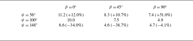
 x/dh
 ∘
 ∘
 ∘
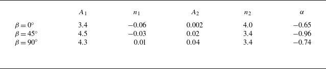
 ∘
 ∘
 ∘


 ∘
 ∘
 ∘

 yz
 ∘
 ∘
 ∘


 x
 ∘
 ∘
 ∘
 x/dh

 x
 ∘
 ∘
 ∘
 x/dh

 yz
 x/dh
 ∘
 ∘
 ∘

 xy
 z/dh
 β
 ∘
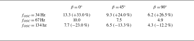
 x/dh
 ∘
 ∘
 ∘

 ∘
 ∘
 ∘
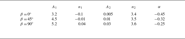
 ∘
 ∘
 ∘

 ∘
 ∘
 ∘

 yz
 ∘
 ∘
 ∘


 x
 ∘
 ∘
 ∘
 x/dh

 x
 ∘
 ∘
 ∘
 x/dh

 θ

 U/Uin

 yz
 x/dh

 z/dh

 U/Uin

 yz
 x/dh



