

INTRODUCTION
The use of parasites as biological ‘tags’ for fish population/stock discrimination has gained recognition as an efficient, cost-effective approach and is being increasingly used worldwide with a noticeable trend towards the use of multivariate statistical techniques considering entire parasite communities (reviewed by MacKenzie, Reference MacKenzie2002; MacKenzie and Abaunza, Reference MacKenzie, Abaunza, Cadrin, Friedland and Waldman2005; Timi, Reference Timi2007). Fish population discrimination using parasites as biological markers is a supervised classification problem. Supervised learning involves building empirical models that relate dependent variable data with known values with independent variables which are then validated by applying to new subsets of data. In spite of its apparent advantages supervised classification has rarely been applied to discrimination of fish populations using parasite data, linear discriminant function analysis (LDA) being the traditional algorithm of choice. However, surprisingly few studies have applied cross-validation of the models (see Ferrer-Castelló et al. Reference Ferrer-Castelló, Raga and Aznar2007 for a discussion).
The size of the datasets and noise are the main obstacles in supervised learning. Thus, a large sample of dependent variable data is required in LDA (e.g. number of cases at least 3× the number of independent variables; see Fabrizio (Reference Fabrizio, Cadrin, Friedland and Waldman2005) for source stock sample size guidelines in LDA for stock identification data analysis). Sample size limitations have led to the adoption of a leave-one-out cross-validation procedure in studies using parasites (e.g. Power et al. Reference Power, Balbuena and Raga2005; Ferrer-Castelló et al. Reference Ferrer-Castelló, Raga and Aznar2007). On the other hand, an inherent characteristic of fish host–parasite data that can increase noise confounding predictive models is the temporal (seasonal, annual) variability in parasite transmission which can result in differential variation in parasite prevalence and/or abundance within individual fish populations. This, translated into signal-to-noise concept in predictive modelling, means that inadequate sampling of the baseline (e.g. communities in fish populations sampled in different seasons) may lead to spurious divergence due to sampling error (noise) being large relative to the actual population divergence (signal). However, replicate sampling that would account for temporal change in parasite communities in fish populations in the development of predictive models is extremely rare (e.g. Ferrer-Castelló et al. Reference Ferrer-Castelló, Raga and Aznar2007; Perdiguero-Alonso et al. Reference Perdiguero-Alonso, Montero, Kostadinova, Raga and Barrett2008) as is the estimation of model performance on independent data (Perdiguero-Alonso et al. Reference Perdiguero-Alonso, Montero, Kostadinova, Raga and Barrett2008).
The weakness of designs lacking independent replicates in fish population discrimination tasks using parasites as sentinels is that models built on a baseline dataset comprising a single sample per population/locality may achieve high predictive accuracy (i.e. assigning fish to their respective samples) but suffer poor generalization capacity (i.e. assigning fish to their populations/geographical areas of origin should the model be applied to subsequent replicate samples). Ferrer-Castelló et al. (Reference Ferrer-Castelló, Raga and Aznar2007) illustrated the problem of the lack of replication, which they considered a type of pseudoreplication, by contrasting results derived from models developed from unreplicated and replicated samples using a carefully designed sampling of a demersal sedentary fish (Mullus surmuletus L.) in the Mediterranean. They found that high inter-sample variability, missed in the unreplicated variant of building the LDA model, clearly confounds differences among localities and concluded that ‘traceability’ (i.e. predicting the harvest location of individual fish) of M. surmuletus based on parasitological data is unreliable at the geographical scale studied.
Random Forests (RF) is an ensemble learning algorithm developed by Breiman (Reference Breiman2001) which builds predictive classification and regression models (forests) by combining multiple classifiers (trees). Each tree assigns a class (vote) to each case in the dataset; the decisions of individual trees in classification are integrated by majority voting i.e. each case is assigned a predicted class which receives the majority of votes. RF generate diversity among the individual classification trees by both randomly changing predictive variable sets and altering the dataset using bagging, an improved method of bootstrap aggregating; this results in building highly competitive models with increased predictive performance (see Breiman, Reference Breiman2001; Svetnik et al. Reference Svetnik, Liaw, Tong, Culberson, Sheridan and Feuston2003; Peters et al. Reference Peters, De Baets, Verhoest, Samson, Degroeve, De Becker and Huybrechts2007; Perdiguero-Alonso et al. Reference Perdiguero-Alonso, Montero, Kostadinova, Raga and Barrett2008 for details and applications). RF offer a number of advantages such as non-linearity of the data, the presence of many zero values, and sample size limitations; the latter can be effectively tackled since RF provide efficient means for model validation. RF are easy to implement, provide insight into the discriminating ability of individual predictor variables and are not prone to overtraining, thus outperforming other machine learning algorithms and traditional statistical modelling approaches (Breiman, Reference Breiman2001; Meyer et al. Reference Meyer, Leisch and Hornik2003; Svetnik et al. Reference Svetnik, Liaw, Tong, Culberson, Sheridan and Feuston2003; Peters et al. Reference Peters, Samson and Verhoest2005; Perdiguero-Alonso et al. Reference Perdiguero-Alonso, Montero, Kostadinova, Raga and Barrett2008). Due to its impressive performance the RF algorithm is increasingly being used in many areas of data mining and modelling (e.g. Lunetta et al. Reference Lunetta, Hayward, Segal and Eerdewegh2004; Koprinska et al. Reference Koprinska, Poon, Clark and Chan2007; Okun and Priisalu, Reference Okun, Priisalu, Martí, Benedí, Mendonça and Serrat2007; Peters et al. Reference Peters, De Baets, Verhoest, Samson, Degroeve, De Becker and Huybrechts2007; Siroky, Reference Siroky2009 and references therein).
Perdiguero-Alonso et al. (Reference Perdiguero-Alonso, Montero, Kostadinova, Raga and Barrett2008) first introduced RF for population assignment of fish using parasite community data. The good discrimination results demonstrated by these authors for Gadus morhua L., which exhibited largely overlapping parasite communities showing annual/seasonal variation, reflect the high potential of RF for developing predictive models using data that are both complex and noisy, thus making the algorithm a promising tool for parasite tag studies. However, the performance of RF was tested on a baseline resulting from a large-scale sampling of a migratory fish and thus the predictive models may have reflected large-scale regional patterns of parasite distribution and community organization (see Timi, Reference Timi2007 for a discussion). It is possible that parasite communities in non-migratory fish change at much lower spatial scales as shown by Ferrer-Castelló et al. (Reference Ferrer-Castelló, Raga and Aznar2007). Interestingly, the studies on both G. morhua and M. surmuletus share a common feature, i.e. reduced accuracy of prediction when models were tested on independent validation sets. Although the differences in the generalization capacity may reflect specific features of these host–parasite systems, the 2 studies provide an important warning on the importance of spatial/temporal replication in inferring population/stock structure from parasite data.
Here, using RF on a large dataset comprising parasite communities in the sparid fish Boops boops (L.) sampled at 5 localities along the northern North-East Atlantic and the Mediterranean coasts of Spain we tested, at different scales, whether patterns of natural spatial and temporal variation can affect the ability to predict multiclass assignment (i.e. allocating individual fish to multiple source populations) of fish population samples. The selection of the model host-parasite system as ‘predictable’ reflects the results of a recent application of supervised learning techniques by Power et al. (Reference Power, Balbuena and Raga2005) addressing the ‘traceability’ of this host in Spanish waters using parasites. These authors obtained excellent classification rates and demonstrated near-perfect classification of samples of B. boops from 2 distant Atlantic (Ondarroa and Malpica) and 1 Mediterranean locality (Burriana) (i.e. 92–96% accuracy depending on the algorithm used). Their study was, however, based on fish sampled in different seasons of the same year (in spring off ondarroa and in winter off Malpica, in both seasons off Burriana); fish sampled off Ondarroa were also considerably larger. Power et al. (Reference Power, Balbuena and Raga2005) admitted that the unbalanced sampling design of their study prevents the assessment of the influence of seasonal or size variation between samples on the allocation of individual fish to its harvest location.
Using much larger and diverse baselines for parasite communities of B. boops sampled within a narrow fish size range, we (i) assessed the spatial and temporal structure of the data by nested subset analysis using binary compositional data at the component and infracomunity levels; and (ii) addressed the effects of scale and temporal change on model generality and spatial resolution by assessment of predictive models in designs with independent replicates using abundance compositional data at the infracommunity level. Our study reveals unexpected variability in the studied host-parasite system with respect to both spatial and temporal scales and illustrates the utility of the RF algorithm for non-migratory fish population assignment using parasites.
MATERIALS AND METHODS
Model host-parasite system
Boops boops (Sparidae) is a demersal to semipelagic non-migratory species common in the North-East (NE) Atlantic and the Mediterranean. The site fidelity of this fish indicates that its parasite communities may reflect food web structure and predator–prey interactions as well as local abiotic conditions which regulate the survival and transmission success of infective stages (Pietrock and Marcogliese, Reference Pietrock and Marcogliese2003) at a finer geographical scale. B. boops hosts a large number of metazoan parasites (67 species, Pérez-del-Olmo et al. Reference Pérez-del-Olmo, Fernández, Gibson, Raga and Kostadinova2007); its parasite communities are diverse and dominated by generalist parasites transmitted from other sympatric fish species.
Parasite community data
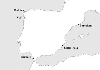
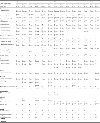
All RF analyses were carried out on parasite abundance data from individual fish which represent replicate habitats for parasite communities (i.e. infracommunities, see Bush et al. Reference Bush, Lafferty, Lotz and Shostak1997). For illustrative purposes one RF model was developed on the total dataset with prevalence data (coding presence and absence of a parasite in individual fish as 1 and 0, respectively). The total dataset comprised infracommunities of 541 fish in 16 distinct fish samples collected in 2005–2006 at 5 localities in the northern NE Atlantic [off Malpica (43°21′N, 8°52′W), Vigo (42°12′N, 8°56′W) and Barbate (36°08′N, 5°55′W)] and Mediterranean [off Santa Pola (37°59′N, 0°36′E) and Barcelona (41°24′N, 2°16′E)] coast of Spain (Fig. 1). Sampling was carried out in late spring (7 samples) and late autumn–winter (9 samples; 2 of these comprise subsamples each taken within a 3-week interval off Vigo and Santa Pola). Seasons are further referred to as spring and winter for brevity; sample sizes are given in Table 1. Only adult fish (standard length range 17–25 cm) were used based on a previous study showing no significant variations with respect to parasite community composition, richness and abundance between host size/age cohorts within this range (Pérez-del-Olmo et al. Reference Pérez-del-Olmo, Fernández, Raga, Kostadinova and Poulin2008). No significant differences in fish size between localities were detected (Kruskal-Wallis ANOVA, H(4, 541)=5·62, P=0·2293). All metazoan parasites were identified and counted. Altogether 30 parasite species from the 5 major higher metazoan taxa were found (prevalence and mean abundance in each fish sample are provided in Table 1); their abundance in individual fish served as independent variables and the locality of sampling was used as the dependent variable in the model development.
Map of the localities where populations of Boops boops were sampled.

Prevalence (%, number above) and mean abundance (±s.d., number below) of parasites and community parameters (bold) in the samples of Boops boops from the 5 localities studied

a Species used in analysis A2 (reduced number of species); b species used in analyses A3-A4 and A8 (species used by Power et al. Reference Power, Balbuena and Raga2005); * species showing significant differences in abundance between localities.
Nested subset analyses were carried out on presence/absence data prior to modelling experiments in order to assess whether significant spatial and seasonal community turnover exists in the model host-parasite system under study. These analyses were carried out at 2 hierarchical scales of community organization: (i) on component community data considering the 14 population samples as independent observations; and (ii) at the infracommunity level based on subsets of 10 randomly selected fish per sample. The Nestedness Temperature Calculator Program was used following Atmar and Patterson (Reference Atmar and Patterson1995). Nonparametric correlation analysis (Spearman's rho, rs) was applied to evaluate the influence of region (Mediterranean-Atlantic) and season of collection (spring-winter) on the rank distribution of parasite communities within the nested matrices.
Classification algorithm
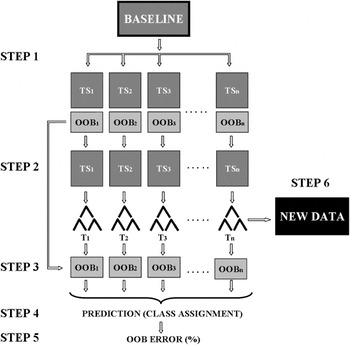
We selected the RF algorithm (summarized in Fig. 2) because it: (i) outperforms other classifiers (e.g. LDA and ANN, Perdiguero-Alonso et al. Reference Perdiguero-Alonso, Montero, Kostadinova, Raga and Barrett2008); (ii) handles data with many zeros; (iii) does not require normality or independence of the predictor variables; and (iv) allows the simultaneous estimation of the error rates using both internal and external validation sets of data. The latter advantage is due to the fact that in RF each tree is ‘trained’ on a bootstrap sample of the training dataset (consisting of ca.2/3 of the dataset) and used to classify the remaining 1/3 cases called out-of-bag elements (OOB) which are not used in the tree construction. The RF algorithm estimates the importance of the predictive variables by measuring the decrease of accuracy, i.e. the increase in the OOB error when OOB data for a given variable are permuted while all other variables are kept unchanged. RF also generate additional useful information about the data, such as a measure assessing the proximity of the data points to one another by counting in how many trees any 2 data points end up in the same terminal node and dividing by the number of trees. This internal measure of similarity between cases in the dataset (forming an N×N proximity matrix with N the number of data points) can be used for graphical analysis of the models using multi-dimensional scaling (MDS) and to detect outliers.
Flow diagram of RF algorithm. Step 1: Generate multiple training subsets (TS) containing ca. 2/3 of cases in the baseline by sampling with replacement (bagging) from the baseline. Leave out of the TS ca. 1/3 of cases (OOB elements) during tree construction to be used for model evaluation/selection. Step 2: Build multiple classifiers (forest of decision trees, T) using TS. ‘Grow’ trees to full length. At each internal node, randomly select a subset from all predictive variables and use the best predictor of this subset to split node. Step 3: Apply each case ‘down’ each tree (from root to leaves) for which it was left OOB to get a classification. Each tree casts a ‘vote’ (i.e. assigns the case to the class corresponding to the leaf). Step 4: Combine the decisions of the individual trees by assigning each case to the class having most of the ‘votes’ (majority voting). Step 5: Compare assigned with actual class labels to obtain estimate of the generalization error of the ensemble of individual trees (=OOB error,% of misclassifications over all OOB elements). Step 6: Predict new data according to the majority vote of the ensemble of trees (forest).

Analytical design
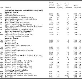
We considered 2 basic classification problems in evaluating the importance of variations in parasite community composition and structure for discrimination of individual fish with respect to the population/locality of sampling: (i) multiclass task (2–5 locality models), using 2 seasonal replicate samples (collected in spring and winter of 2005) from each of the localities; and (ii) 2-class task, using 4 seasonal replicate samples (collected in spring and winter 2005 and 2006) from 1 Atlantic (off Vigo) and 1 Mediterranean (off Santa Pola) locality. Within these tasks a series of analyses were designed addressing the importance of scale (i.e. geographical extent) and temporal variation (‘noise’) on RF model development and the resolution of fish assignment. We developed predictive models using only the data in the training sets and assessed their performance on the internal OOB datasets and in the majority of runs on independent validation sets which were not used in any way in model construction. Details of the datasets and analyses are provided in Table 2.
Details of the analyses and datasets used

a Validation set only; b OOB set only; c two validation sets; OOB, internal validation dataset; VS, external validation set.
(i) First, we assessed the accuracy of RF using both OOB and validation set in 2 analyses (labelled A1 and A10 in Table 2). Each analysis comprises 20 models built using a different random seed each time so that different models are produced. Each time the dataset was randomly and uniformly (i.e. maintaining the same proportion of classes as in the total dataset) split into a training (80% of total) and an independent validation set (20%). This subdivision reflected an attempt to comply with a minimum sample size that would be representative in future application of the models. Each model was then evaluated on the OOB set and the validation set. The results were averaged over these 20 independent models.
(ii) We then examined the effect of reducing the number of predictor variables in 2 analyses (A2 and A3) comprising 20 models each using random OOB and validation sets as described above. In A2 only species with a prevalence in the total dataset >5% were included (marked with an ‘a’ in Table 1) and A3 was carried out with the 6 variables (i.e. abundance of the 6 species marked with ‘b’ in Table 1) used by Power et al. (Reference Power, Balbuena and Raga2005) thus providing comparative data to their study. In the latter case a ‘control’ LDA model (A4, with a random validation set as in A3) was built with the dataset used for the RF model to ensure the lack of bias due to the new learning algorithm applied here.
(iii) We also built a series of models (A5-A9) using simplified 2, 3 and 4-class tasks to both address the question of scale/spatial extent and examine the performance of RF in relation to increased complexity of the classification problem. Within the 4-class task 2 spatial configurations were examined each including samples from one of the 2 closest NE Atlantic localities, Vigo (A5) and Malpica (A6). One of these analyses (A8) in the 3-class task (including samples from Malpica, Barbate and Barcelona) was carried out with the variables used by Power et al. (Reference Power, Balbuena and Raga2005).
(iv) We addressed issues of temporal seasonal variation in a set of experiments (labelled A11-A20 in Table 2) designed within the 2–5 class tasks with training and validation sets comprising fish sampled in different seasons in 2005. Data for a few species absent in either the spring or winter set were excluded from the analyses; in each case control runs with all species confirmed that this omission had no effect on the predictive power of the models. Finally, within the 2-class task (samples from 2005 and 2006) the temporal (both seasonal and annual) variation in parasite communities was assessed in 6 individual runs with different configurations of training and validation sets (labelled A21-A26 in Table 2). Of these, 2 analyses were aimed at a comparison of the results using pooled data (A24) and 2 replicate fish samples taken within a 3-week interval in winter 2006 as independent validation sets (A25).
Prior to experiments, the learning performance of RF was studied in a series of runs in order to optimize the 2 user-defined parameters: the number of trees (ntree) and the number of randomly selected variables to split the nodes (mtry). The following configuration was selected for building RF models: ntree=2000; mtry=√No. of variables (default); using tuneRF option did not show departures from the default value of mtry. RF models were developed with randomForest package (version 4.5–28) and LDA models were obtained using the lda progam (MASS package) in R.2.8.1 statistical software (Liaw and Wiener, Reference Liaw and Wiener2002; Reference Liaw and Weiner2007; Venables and Ripley, Reference Venables and Ripley2002; R Development Core Team, 2009 (http://www.R-project.org)).
Parametric statistical analyses (univariate and multivariate analysis of variance (ANOVA, MANOVA)) were performed on arcsin√p transformed prediction accuracy data (expressed as proportions) and log10 (x+1) transformed abundance, respectively (Sokal and Rohlf, Reference Sokal and Rohlf1995) using Statistica 6.0 (StatSoft, Inc., Tulsa, OK, USA).
RESULTS
Data complexity
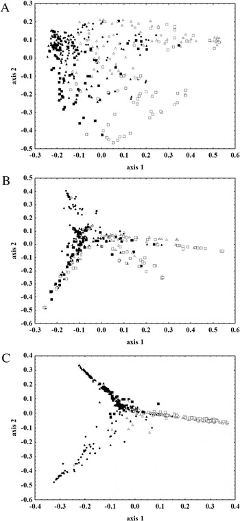
Fig. 3 shows one unsupervised (i.e. the population of origin unspecified, Fig. 3A, which reveals the structure of the unlabelled data) and 2 supervised multidimensional scaling plots (1 based on parasite presence/absence and 1 on abundance; Fig. 3B–C) of the entire dataset using proximity matrices produced in RF as measures for similarity between parasite communities in individual fish. The plots illustrate the complex structure of the dataset, as reflected in both high dispersion and overlap between infracommunities in the 5 fish population samples. The RF algorithm appears to handle presence/absence data well although the model showed lower overall accuracy (68%; Fig. 3B) than that built on abundance data (78%; Fig. 3C). The difficult structure of the entire dataset was confirmed by a MANOVA which revealed differences in parasite abundance distributions with respect to both locality (F(120, 1314)=15·88, P<0·0001) and season (F(30, 330)=29·87, P<0·0001) and a significant interaction (F(120, 1314)=6·71, P<0·0001). Univariate comparisons of abundances of individual parasite species identified 21 species (marked with a ‘*’ in Table 1) potentially useful for discrimination between fish populations; however, the abundance distribution of most taxa was affected by a significant interaction between locality and season (12 species, typically > 80% of the species in each pairwise comparison).
Multidimensional scaling plots (MDS) of the entire dataset. (A) Unsupervised MDS plot based on proximities between cases (parasite infracommunities) in RF developed without specification of the locality. (B) Supervised MDS plot (based on proximities computed from parasite presence/absence data). (C) Supervised MDS plot (based on proximities computed from parasite abundance data). Symbols for communities in individual fish: filled squares, fish sampled off Malpica; filled triangles, fish sampled off Vigo; filled diamonds, fish sampled off Barbate; open triangles, fish sampled off Santa Pola; open squares, fish sampled off Barcelona.

A nested subsets analysis provided support for the existence of significant nested patterns in parasite communities in the 5 host populations over the 2 seasons of sampling (component communities: T=29·1°, P<0·0001; infracommunities: T=11·5°, P<0·0001). Both analyses showed 2 common features. First, the overall order of communities (poorest to richest) in the packed matrix appears to reflect a Mediterranean-Atlantic contrast with those from the Mediterranean being poorer (correlations between the rank position of communities and the region coded as 0 and 1, respectively: rs=0·677; P=0·008 and rs=0·457; P=0·0001 for component and infracommunities, respectively). Secondly, the order of the communities indicates a temporal effect on parasite species composition since there was a highly significant correlation between the rank position in the packed matrix and season (rs =0·384; P=0·0001) for the random infracommunity dataset, winter communities being overall poorer subsets of those sampled in spring; the former were also characterized by a lower mean abundance (see Table 1).
Spatial resolution: scale and configuration
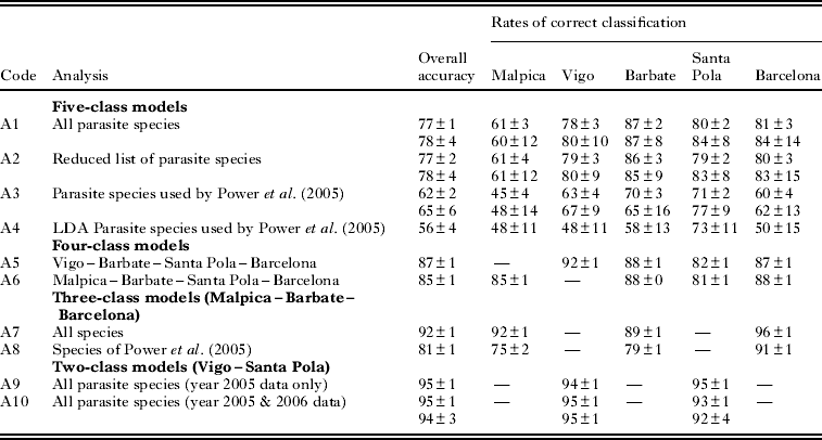
A summary of the analyses by means of accuracy and rates of correct classification of fish per locality is provided in Table 3. Our results revealed 4 important points with respect to the complexity of the datasets and the scale of the classification problem under consideration. First, the OOB estimation of accuracy in RF appears as reliable as that obtained using an independent validation set as evidenced by the extremely close values for analyses in both 5-class (A1-A3) and 2-class (A10) tasks; we, therefore, used no external validation sets in analyses A5-A9. A number of good models were developed with RF within both tasks with accuracy higher than the means given in Table 3. Thus 30% of the 5-class models (A1) had an overall accuracy >80% (87% for the best model) and 35% of the 2-class models (A10) had an accuracy >96% (99% for the best model).
Summary of the analyses addressing the effect of data and problem complexity
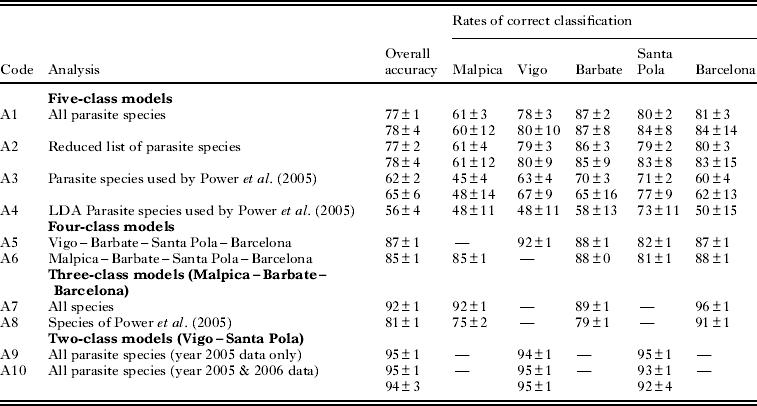
Secondly, although a reduction in the number of variables from 30 to 19 did not affect the accuracy (A1 vs A2 in Table 3), a drop to 6 variables resulted in a substantial decrease (on average 15% and 13% for the OOB and validation set, respectively; A1 vs A3). The lack of difference in the first case is probably due to the fact that the species not used in the analysis had the lowest occurrence in the dataset and subsequently the lowest importance in building RF models. However, the reduction in the second case was actually a selection of the variables used in a previous study by Power et al. (Reference Power, Balbuena and Raga2005). We, therefore, developed a ‘control’ LDA model (A4) which showed a similar degree of error (on average 20% decrease in accuracy as compared to the mean of 20 LDA models using all variables; data not shown). Thus, it appears that the increase in the error rates using 6 variables is not an artefact due to the different algorithm used by us. This is supported by the fact that using the same variables in the simplified 3-class task (A8) also resulted in a decrease in accuracy albeit lower (11% on average). Notably the overall accuracy of the 3-class model developed with all variables was, on average, 15% higher than in the 5-class task (A7 vs A1, see Table 3) and similar to that observed in the 3-class task but with a different set of localities in the study of Power et al. Reference Power, Balbuena and Raga(2005).
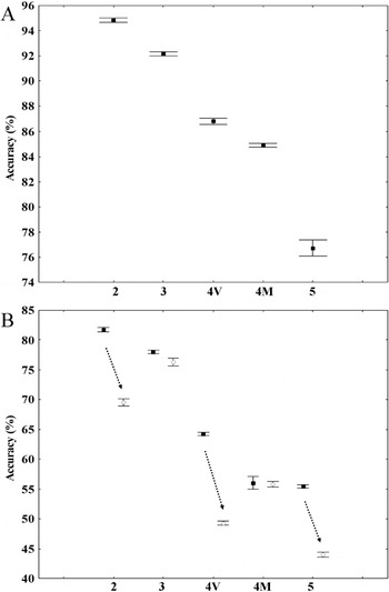
Thirdly, a comparative examination of model efficiency along the gradient of populations examined here (i.e. 2–5 class tasks) showed that the performance of RF is strongly dependent on the spatial extent and configuration of the problem in the host-parasite system under study. Fig. 4A illustrates a gradual decrease in overall accuracy (estimated from OOB error rates in 20 models each in A9-A7-A5/A6-A1, see Table 3) along this gradient at a constant maximum number of variables. The models of the two 4-class tasks although with different configuration (each including one of the close Atlantic localities in the 5-class task, Malpica and Vigo) exhibited a similar decrease in accuracy as compared to the 3-class task models (Table 3); their accuracy was also, on average, 8–10% higher in comparison with the 5-class models. A summary of the most important variables used in the 2–5-class models revealed that 5 species were most frequently used in model development: Hemiurus communis Odhner, 1905, Aphanurus stossichii (Monticelli, 1891), Lecithocladium excisum (Rudolphi, 1819), Prosorhynchus crucibulum Rudolphi, 1819 and Tormopsolus sp.; the first 2 being the most important. All 5 species also exhibited significant differences in abundance the first 3 generally contrasting Atlantic vs Mediterranean samples and the last 2 discriminating samples from Barbate from the rest.
Boxplots of accuracy of classification (means±95% confidence limits) along the gradient of complexity (i.e. from 2 to 5 populations modelled as indicated by numbers on X axis). (A) Accuracy estimated from OOB error rates in 20 models for each configuration (from left to right: experiments A9–A7–A5/A6–A1). (B) Accuracy estimated from error rates for the independent validation sets in 20 models for each configuration (from left to right: experiments A20/A19–A18/A17–A14/A13–A16/A15–A12/A11). The two different configurations of the 4-class task are denoted as: 4 V (Vigo – Barbate – Santa Pola – Barcelona) and 4M (Malpica – Barbate – Santa Pola – Barcelona). Filled squares indicate accuracy in models built with a training set of Winter samples and validated on Spring samples. Open circles indicate accuracy in models built with a training set of Spring samples and validated on Winter samples. Arrows point to the significant drop in accuracy in the Spring vs Winter models built on datasets which included samples from off Vigo. All models were developed for the 2005 dataset.

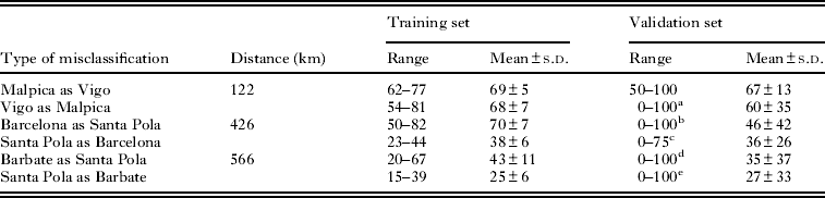
Generally, the rates of correct classification per locality were close to the mean overall accuracy values with exception of those for Malpica in the 5-class task (Table 3); fish from this locality being most heavily misclassified. An examination of the misclassification rates in the models within this most complex task (A1) revealed that they are highest between the samples from the 2 closest localities (Malpica and Vigo) in the Atlantic (on average 2/3 of all misclassified fish per locality; Table 4). There was a significant negative correlation between the mean misclassification rates in the validation sets and the geographical distance between localities (rs=−0·96, P=0·003). In fact, the models based on configurations lacking one of the pair of the closest locations in each region (i.e. Malpica-Vigo in the Atlantic and Barcelona-Santa Pola in the Mediterranean; A5, A6, A7, A9) showed a considerable improvement of the classification of fish from the other location in the pair (8–31% increase, Table 3).
Misclassification rates (expressed as % of all misclassified fish per locality) for samples collected from geographically closest localities
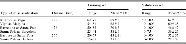
a 0 in 2 models; b 0 in 6 models; c 0 in 7 models; d 0 in 10 models; e 0 in 9 models.
Temporal variation
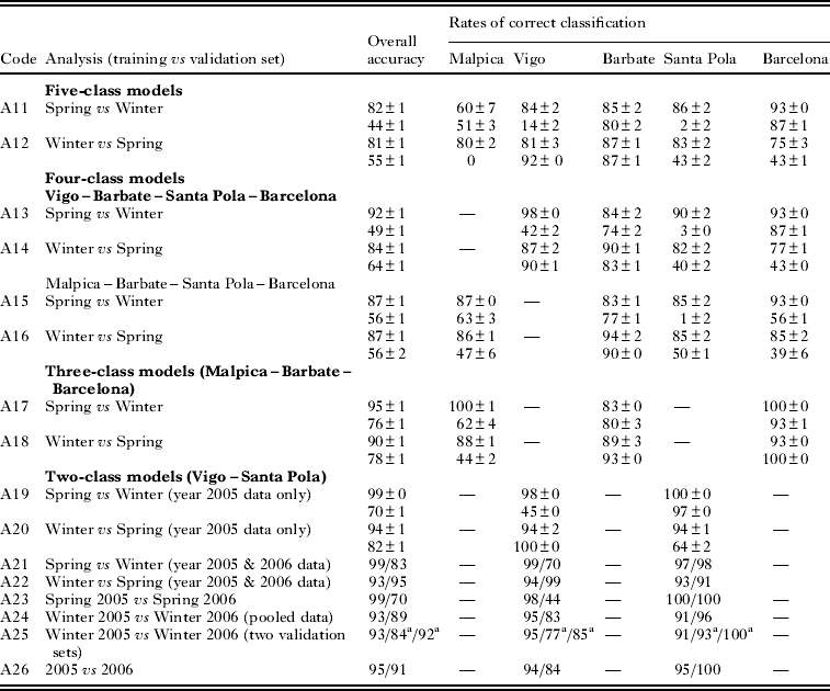
Using samples from 1 season only for model development resulted in a slight increase in the accuracy of the classification of the training set (by 4–5% in the 5-class task; by 2–5% in the 4-class task; by 2–3% in the 3-class task; and by 1–4% in the 2-class task, compare Table 3 and Table 5). However, using a validation set comprised of samples collected from the other season invariably led to a substantial drop in accuracy in 3–5-class models. Using spring samples for training resulted in a higher decrease in accuracy in all tasks in contrast to the models developed using winter samples for training: (i) on average by 38% (A11) vs 26% (A12) in the 5-class task; (ii) on average by 31–43% (A13-A15) vs 20–31% (A14-A16) for the 2 configurations in the 4-class task; (iii) on average by 19% (A17) vs 12% (A18) in the 3-class task. There was, on average, a 29% (A19) vs 12% (A20) decrease in the 2-class task using data from 2005 only and a 16% decrease (A21) vs 2% (A22) increase for the 2-class task using the pooled data from both years.
Summary of the analyses addressing the effect of the temporal variation
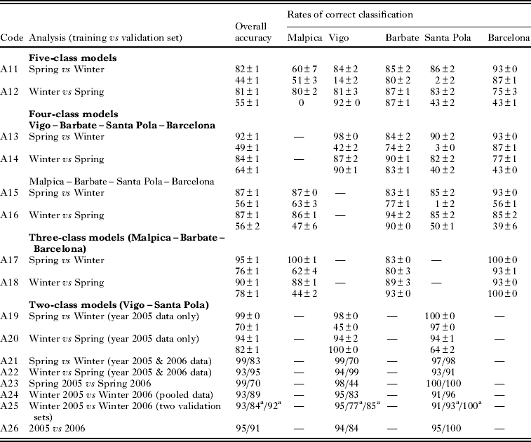
a Two validation sets.
A plot of the mean accuracy of prediction based on the 2 different validation sets of the above tasks (Fig. 4B) shows a trend of decreasing predictive power as the complexity of the problem (i.e. number of populations) increases, similar to that observed in Fig. 4A. ANOVA on these data (R2=0·979; overall F=28·61, P=0·0012) revealed a highly significant effect of the complexity of the problem modelled (F=35·39, P=0·0009) and a significant effect of the season of collection of training samples (F=8·27, P=0·035). These results clearly indicate that the viability of the predictive models developed on a single season baseline is affected by substantial seasonal differences in infracommunities in B. boops from the 5 populations studied. Moreover, a pattern of large disparity between the overall predictive power of models built on datasets including samples from off Vigo (Fig. 4B) was observed, with a much higher accuracy of assignment in the models using winter samples for training; in the latter models the rates of correct classification of fish from off Vigo were also higher in the validation sets; this indicates the influence of the spatial configuration of the populations being modelled.
An examination of the variable importance in the models developed from seasonal datasets in the 3–5-class tasks revealed a clear spring-winter segregation of the species lists representing the 5 most important variables. H. communis, A. stossichii and P. crucibulum were most frequently used in the models built on the spring training datasets, whereas L. excisum, Hysterothycium aduncum (Rudolphi, 1802) and Tormopsolus sp. had higher importance in those developed on the winter datasets. A somewhat ‘diluted’ pattern was observed in the 2-class task (A19-A22) with A. stossichii constantly having the highest rank with respect to importance followed by H. communis and juvenile lepocreadiids in the models developed on spring datasets.
The effect of the annual variation in parasite communities on model development was addressed for the 2-class task (Vigo-Santa Pola) for which we possessed 2 seasonal samples for both 2005 and 2006. The model developed with training data from spring samples of 2005 resulted in a 29% decrease in accuracy when tested on samples collected in spring 2006, which was in sharp contrast to the model obtained using winter samples (4% decrease, pooled data; A23 vs A24 in Table 5) due to poorer prediction of fish sampled off Vigo in both cases. Using 2 validation sets for the latter ‘winter configuration’ (A25) revealed some small differences in the accuracy (3–5% as compared to the model developed with the pooled data) but generally good classification with a similar pattern of higher variability in assignment of fish sampled off Vigo. Finally, the model built on the data from 2005 and validated on the samples of 2006 provided an excellent classification with a similar resolution to those obtained using pooled seasonal samples from either the first or both years of sampling (i.e. A26 vs A9-A10 in Tables 5 and 3, respectively).
DISCUSSION
The main results of this study are the following: (i) RF algorithm is well suited for multiclass fish population assignment using parasite communities as biological markers and can be recommended for discovery of classification rules for populations of non-migratory fish; (ii) RF provides an efficient means for model cross-validation on the training data and this allows sample size limitations in parasite tag studies to be tackled effectively; (iii) The performance of RF (and perhaps of other classifiers) is dependent on the complexity and spatial extent/configuration of the problem; (iv) The development of predictive models is strongly influenced by seasonal change in host–parasite systems and this stresses the importance of both temporal replication and model validation in parasite tagging studies; and (v) These potential problems can best be solved by using the RF algorithm as it builds models with high generalization power on diverse baselines that incorporate seasonal samples.
Using fish of comparable narrow size-range we have considered 2 mechanisms for assessing the ‘predictability’ of the host-parasite system studied. We used the advantages of the RF algorithm to develop predictive models for assignment of individual fish in designs with both internal and external validation and multiple replicate samples. Our study uncovered previously unsuspected levels of variation among infracommunities in B. boops which affect the accuracy of the allocation of individual fish to their harvest location and this was in contrast with our initial expectations. Nevertheless, the first set of models confirmed that RF provide very good prediction results when applied to parasite abundance data despite the problems with these markers, such as the aggregated abundance distributions of parasites resulting in the presence of many zero values. Our study thus extends the applicability of RF to non-migratory fish host-parasite systems. The fact that the algorithm does not overfit (Breiman, Reference Breiman2001; Svetnik et al. Reference Svetnik, Liaw, Tong, Culberson, Sheridan and Feuston2003; Prinzie and Van den Poel, Reference Prinzie and Van den Poel2008) confirmed here by the lack of difference in the accuracy estimates based on internal and external validation may be very useful for predictive modelling of parasite datasets. Since RF produce an unbiased internal estimate of the test set error, there is no need for an external validation set during model development (providing that enough trees have been grown, see Breiman, Reference Breiman2001; Liaw and Wiener, Reference Liaw and Wiener2002). This, in fact, allows a reduction of baseline sample size thus making the parasite community approach to fish population discrimination more cost-effective. For example, this reduction of the present baselines would have been 20% (on average communities in 15 fish per locality which we used for model validation on independent datasets); still a reliable baseline would require a minimum of 2 seasonal samples of parasite communities (on average 25 fish per locality each).
One important aspect of our study is that whereas the implementation of predictive modelling is straightforward when only 2 fish populations are included, it becomes more complicated when the classification problem involves a larger number of populations. Our results indicate that (i) RF generalize better with a large number of variables; (ii) the species used by Power et al. (Reference Power, Balbuena and Raga2005) for a different set of localities do not provide the same resolution; and (iii) the performance of RF is dependent on the number of populations and scale (i.e. spatial extent) of the contrasts. Although parasite dynamics in individual fish populations typically vary over space, the amount of parasite community disparity among populations can affect assignment. Parasite community distinctness was more apparent as the distance between source populations increased. Its effect on prediction was especially pronounced in the models contrasting Atlantic and Mediterranean locations (2-class tasks but also in the 3-class task, Barbate being located in the area of transition between the two regions (see e.g. Rueda and Salas, Reference Rueda and Salas2003; Pérez-del-Olmo et al. Reference Pérez-del-Olmo, Fernández, Raga, Kostadinova and Morand2009) due to higher spatial species turnover rates. The significantly non-random community structure observed in our study although reflecting high compositional overlap also indicates the effect on predictive models of differential distributional and/or colonization patterns in parasites of B. boops on a broad spatial scale. This resulted in high prediction accuracy of classification of B. boops populations in the Mediterranean-Atlantic contrast (i.e. 2–3 class tasks) which corresponds to the levels reported by Power et al. (Reference Power, Balbuena and Raga2005). Similarly, the existence of a large-scale latitudinal gradient influencing the distribution of parasites has resulted in their successful use as tags for the delineation of different populations/stocks of their fish hosts in the South-West Atlantic (reviewed by Timi, Reference Timi2007). On the other hand, fish assignment from geographically close populations was less accurate and this affected the predictions in the most complex task. This fact can be associated with the significant spatial synchrony of the assemblages of the most prevalent and abundant (‘core’) parasites of B. boops indicating a close-echoing environmental autocorrelation that declines with distance (Pérez-del-Olmo et al. Reference Pérez-del-Olmo, Fernández, Raga, Kostadinova and Morand2009). Our results, therefore, clearly show that the host-parasite system studied is not as predictable as suggested by Power et al. (Reference Power, Balbuena and Raga2005). The degradation of the classification accuracy suggests that the minimum spatial resolution for population delimitation in this system scale down to ca.150 km, and this highlights the importance of both scale and spatial configuration in tagging studies on non-migratory fish populations using parasites.
To the best of our knowledge our study is the first to address, in detail, the effects of temporal change on fish population assignment using parasites by scrutinizing the predictive models in designs with independent replicates and external validation. Although the accuracy of assignment using the total baseline in the 3-class task was similar to the data by Power et al. (Reference Power, Balbuena and Raga2005), the models with external validation developed on the seasonal datasets indicate that substantial seasonal differences in infracommunities in B. boops from the 5 localities exist which jeopardize the development of viable predictive models. The poorer predictive power of the models built on the spring samples can be linked to the distinctly higher frequency of occurrence (in addition to abundance) of the variables in the training than in the validation set. Seasonal changes in species richness, abundance and structure of benthic macroinvertebrate communities (e.g. Arias and Drake, Reference Arias and Drake1994), and mollusc assemblages in particular (Rueda and Salas, Reference Rueda and Salas2003 and references therein), in the shallow vegetated habitats of B. boops have been reported along both Mediterranean and Atlantic coasts of Spain. Repetitive seasonal trends with higher richness and abundance in molluscan assemblages in the warm (spring and summer) vs cold (autumn and winter) season (e.g. Rueda and Salas, Reference Rueda and Salas2003) can affect transmission rates of the main bulk of parasites of B. boops (17 digenean species) since these require a mollusc host to complete their life cycles. This is supported by the non-random nested patterns observed in our study which reflect seasonal community turnover at the infracommunity level. Notably, the models in the 2-class task revealed a repetitive pattern with a more pronounced effect of annual variation on prediction of spring communities. In a study on the decay of similarity with distance on a larger spatial/sampling scale Pérez-del-Olmo et al. (Reference Pérez-del-Olmo, Fernández, Raga, Kostadinova and Morand2009) detected inconsistent spatial patterns of parasite communities in B. boops across seasons with a significant spatial autocorrelation in spring as opposed to the lack of spatial synchrony during the cold season; this can explain the better performance of the models developed on winter baselines. However, although winter baseline datasets alone appear to be better suited for the development of good models, approaches using complex baselines incorporating seasonal samples have clearly shown that RF achieve better generalization (i.e. the models could take into account the variability of parasite infracommunity data effectively) for the non-migratory fish host-parasite system studied; in this case the baseline data need not to be re-established annually. Finally, our results based on independent replicate samples provide empirical evidence that temporal confounding may cause serious problems to formal interpretation of parasite tagging studies which use only 1 replicate sample per population/locality.
In conclusion, our results suggest that, from a technical point of view the RF algorithm is well suited to multiclass fish population assignment using parasites as biological markers thus extending its applicability to non-migratory fish. We believe that, in addition to parasite tag studies, RF have an important potential for multisource evidence approaches incorporating e.g. genetic and phenotypic (morphometry, otolith shape/elemental composition) markers in applications for population allocation of individual fish which will continue to develop in fisheries.
FINANCIAL SUPPORT
The study was supported by a Alexander von Humboldt Foundation Fellowship (A.P.O.); Institute of Parasitology (Academy of Sciences of the Czech Republic) (A.K., grant numbers Z60220518, LC522); and CTM2006-07106/MAR-FEDER grant and I3 Contract from the Ministry of Science and Innovation of Spain (M.F.).