

Introduction
The creation and use of a crop descriptor list, an assembly of varying plant characters, has been promoted by Bioversity International to characterize and evaluate plant genetic resources. Each descriptor, a trait, has corresponding ‘descriptor states’ which are distinguishable states of expression of the specified trait that potentially represent all the observed trait variations of the entire species (Bioversity International, 2007). The clear and definite representation provided by the descriptor list facilitates ease in universally describing plant germplasm collections for their subsequent utilization. As of 2018, there are 102 descriptor lists of various crops published by Bioversity International; however, many crop species have no established crop descriptors, limiting their formal characterization. Limitations include the use of subjective assessment in establishing these lists, as highlighted by Gentallan et al. (Reference Gentallan, Altoveros, Borromeo, Endonela, Hay, Lalusin, Reaño and Yoshioka2019) in proposing a systematic protocol of colour descriptor state formulation. Particularly for traits with irregular shapes, there is difficulty in accurately identifying clear and definable states due to ambiguity in the process of representation. To address this, several image-based phenotyping techniques have been used to characterize the shapes or plant organs such as fruits (Wycislo et al., Reference Wycislo, Clark and Karcher2008), flowers (Neto et al., Reference Neto, Grossi and Pinto2009) and seeds (Cervantes et al., Reference Cervantes, Martín and Saadaoui2016). These include the use of elliptic Fourier analysis (EFA) that analyses closed contours immaterial of the size and configuration (Kuhl and Giardina, Reference Kuhl and Giardina1982). This method describes mathematically the overall shape of an object by transforming outline information into Fourier coefficients. Plant characterization using this method was first attempted by White et al. (Reference White, Rentice and Verwist1988) who analysed the leaf shape of Betula. Since then, several studies of plant shape characterization using EFA have been published, for example, such as in the case of petal shape in Japanese primrose (Yoshioka et al., Reference Yoshioka, Iwata, Ohsawa and Ninomiya2004), grain shape in rice (Iwata et al., Reference Iwata, Ebana, Uga and Hayashi2015) and fruit shape in persimmon (Maeda et al., Reference Maeda, Akagi and Tao2018). Moreover, in defining qualitative descriptors, such as shape and colour where subjectivity often occurs, the ‘use of image analysis eventually to convert qualitative data to quantitative data’ has been encouraged (Bioversity International, 2007). In spite of this, there are no reports on the application of image-based techniques, particularly EFA, to systematically establish shape descriptor states.
Pili (Canarium ovatum Engl.), a native tree nut of the Philippines with great economic potential (Coronel, Reference Coronel2011), shows kernel shape variation but has no established descriptor list. Thus, this study aimed to objectively identify the shape descriptor states by elliptic Fourier descriptors using pili (C. ovatum Engl.) kernels as a model.
Materials and methods
Plant materials
The plant materials consisted of 53 pili accessions from the Institute of Crop Science, and the National Plant Genetic Resources Laboratory of the Institute of Plant Breeding, College of Agriculture and Food Science, University of the Philippines Los Baňos. Each accession was represented by 10 samples. To avoid shape and size variation due to varying seed moisture contents (mc), samples were air dried to approximately 5% mc prior to image acquisition.
Image acquisition
Kernel images were captured using the Videometerlab3 set up (Videometer A/S Hørsholm, Denmark). To ensure standardized and comparable images, the set up was calibrated for colour, geometry and self-illumination using standard uniform bright, uniform dark and geometric discs. Samples were then placed on a blue background disc, and images with a size of 2056 × 2056 pixels and a resolution of ~45 µm/pixel were captured using the set up.
Computation of elliptic Fourier coefficients
A modified method developed by Yoshioka et al. (Reference Yoshioka, Iwata, Ohsawa and Ninomiya2004) to analyse shape variation through EFA was used. Prior to analysis, the images were formatted into 24-bit bitmap (*.bmp) using SigmaScan®Pro 5.0 software. The converted images were chain-coded and normalized using Shape version 1.3 software (Iwata and Ukai, Reference Iwata and Ukai2002). Initially, using the ChainCoder of Shape ver. 1.3, closed contours of the kernel and seed were obtained from the binary images. The contours were then chain-coded using the method proposed by Freeman (Reference Freeman1974). The pixel contour of the digital images served as the discrete approximation of a continuous curve and was recorded as chain codes to describe the geometrical information on outlines ranging from 0 to 7. From the chain codes, the elliptic Fourier coefficients of the n th harmonic (a n, b n, c n, d n) were computed to describe the shape variations in the pili accessions. Twenty (20) harmonics were used as they were considered to be sufficient in describing shape variations for morphological analysis (Yoshioka et al., Reference Yoshioka, Iwata, Ohsawa and Ninomiya2004; Sayinci et al., Reference Sayinci, Kara, Ercişli, Duyar and Ertürk2014). Then, the computed Fourier coefficients were standardized for size, orientation and starting point variations using the method of Kuhl and Giardina (Reference Kuhl and Giardina1982).
Image-based characterization of pili kernel physical properties
To validate the descriptor formulated states, the projected area (A, mm2), length (L, mm), width (W, mm) and perimeter (P, mm) of each kernel and seed were determined using VideometerLab 3 software. Subsequently, from the image-based measurements, roundness (R), pointness (Po), elongation (El), eccentricity (Ec) and compactness (C) were calculated using the equations in online Supplementary Table S1.
Principal component analysis, cluster analysis and visualization
From the elliptic Fourier coefficients of the sample outlines, principal component analysis was performed using the variance–covariance matrix to obtain fewer, uncorrelated variables that would effectively summarize the variation observed in the coefficients (Rohlf and Archie, Reference Rohlf and Archie1984). The data were analysed in R Version 3.4.3. Using Perl Strawberry version 5.26.1.1, normalized elliptic Fourier descriptors were converted to dat format, for R software readability. The scores of the components were computed using the package SHAPE on R (Iwata and Ukai, Reference Iwata and Ukai2002) and used as shape characteristics for succeeding analyses. The dendrogram was created using unweighted pair group method with arithmetic means (UPGMA) and sequential, agglomerative, hierarchical and nested clustering parameters (SAHN) program of Numerical Taxonomy and Multivariate Analysis System (NTSYS)-pc version 2.1 (Rohlf, Reference Rohlf2002). The dendrogram was cut into clusters based on the variance within and between clusters. As a general rule, the dendrogram was statically cut at the point where the minimum number of clusters satisfies the following conditions: variance within clusters is ⩽11% and any additional cluster will entail <2% decrease in the variance within clusters. This will minimize variance within clusters and maximize any additional benefit of added variance between clusters by adding an additional cluster. The variances were computed using XLSTAT 2016 (Addinsoft, Inc., Brooklyn, NY, USA). From the generated clusters, shape Fourier coefficients were averaged within clusters. The averaged values per cluster were used to represent a descriptor state. The averaged cluster values for the principal component values were visualized using the draw functions of the package SHAPE on R (Iwata and Ukai, Reference Iwata and Ukai2002).
Analysis of variance (ANOVA), multivariate ANOVA (MANOVA) and pair-wise mean comparisons
To examine the differences in physical properties among accessions, ANOVA at 5% level of significance was performed for each physical property. If at least one treatment was considered to be different, an LSD test was conducted to distinguish the differences between treatments. For the kernel outline differences between clusters, MANOVA at 5% level of significance was performed. Upon observing a significant difference between clusters, pairwise comparisons from Fisher distance and P values were calculated at the same level of significance.
Linear discriminant analysis (LDA)
To validate further the descriptor states, a separate set of 20 kernel outlines per cluster was evaluated using LDA. Per cent correct classification rates between clusters were used to gauge the accuracy of discriminating individual outline shapes based on the clusters. LDA was implemented using XLSTAT 2016 (Addinsoft, Inc.).
Results
The first principal component accounted for 92.94% of the total variation; 98.62% of the total variance could be explained by the first three components (Figs. 1 and 2). It was determined that the first principal component accounts for the variation in length to width ratio; whereas, the second and third principal components explain the variation in the location of the widest portion and the truncation of the apex and base of the kernel, respectively (Fig. 1).
Shape variations explained by the first three principal components; SD indicates standard deviation.

Plot of component loadings obtained from PC1 and PC2 for the 53 pili accessions; clusters are enclosed by concentration ellipses.

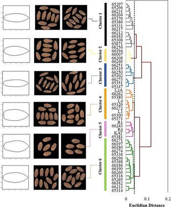
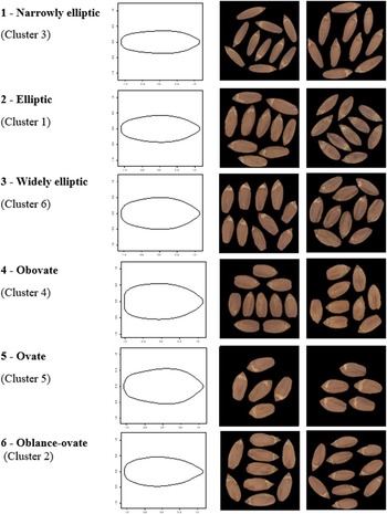
From the variance within and between clusters with an increasing number of classes, it was determined that five clusters will impose 9.40% variance within clusters; furthermore, an additional class will result only to an additional decrease of 1.37%. Hence, the dendrogram was truncated to produce six clusters corresponding to six descriptor states for kernel shape – narrowly elliptic, elliptic, widely elliptic, ovate, obovate and lance-ovate (Figs. 3 and 4).
Dendrogram of 53 pili accessions from average elliptical Fourier coefficients of shape outlines.

Pili kernel shape descriptor states.

With a low Wilk's Lambda of 0.033, significant differences among the six clusters were observed based on the kernel outlines (Table 1). The pair-wise comparisons between the six clusters displayed significant levels of difference indicating an effective classification based on kernel outlines. From the pre-classified kernel outlines, the discriminant analysis showed 95.00% correct classification (Table 1). The highest classification was observed for cluster 3 with 100% and the lowest was observed at cluster 6 with 90.00%. Furthermore, highly diverse accessions were observed for all the physical shape parameters with an H' of >0.67 (online Supplementary Table S2).
Differences between clusters based on kernel outlines and their per cent correct classification from discrimination analysis of individual kernel outlines

Values displayed in bold are significant at the level alpha = 0.003.
Discussion
Clusters 3, 1 and 6 represent the elliptical series of shapes – narrowly elliptic, elliptic and widely elliptic, respectively (Figs. 3 and 4). Showing non-overlapping points across PC1, these three clusters are highly influenced by the first principal component and are easily discriminated through the principal coordinate analysis of the first two components (Fig. 2). The states match with the described shape classification of the elliptic series of shapes by Simpson (Reference Simpson and Simpson2010). The three states are considered elliptic as the widest part is located at the midpoint of the kernel and the margins are curved; however, variation in length to width ratio is observed. From narrowly to widely elliptic, the length to width ratio decreases. The three states were well represented in the germplasm collection with 15, 13 and seven accessions having widely elliptic, elliptic and narrowly elliptic kernel shapes, respectively (Fig. 4).
Cluster 2 is characterized to have an oblance-ovate shape, also known as inverted lachryform or tear-shaped. This shape has curved margins that are widest near the base and the length to width ratio is between 3:1 and 2:1 (Simpson, Reference Simpson and Simpson2010), indicating a high length to width ratio. This cluster is highly influenced by the second principal component with the movement of the widest point from the centre to near the apex (Fig. 1). Thus, accessions from this state were completely separated at PC2 in the principal coordinate analysis (Fig. 2). Inverted lachryform shapes, however, are only represented by four accessions in the germplasm collection (Fig. 3).
Clusters 4 and 5 represent ovate and obovate shapes, respectively. Having longer widths, they are differentiated in the first principal component by their relatively lower length to width ratio ranging from 2:1 to 3:2 (Simpson, Reference Simpson and Simpson2010). These shapes are differentiated from each other in the second principal component. Obovate-shaped accessions have the widest point near the apex, whereas the ovate-shaped accessions have widest points near the base as shown in the second principal component (Fig. 2).
Using the validation set, a relatively high correct classification rate was observed compared to the 34.9% correctness in classifying hazelnut outlines based on cultivars by Sayinci et al. (Reference Sayinci, Kara, Ercişli, Duyar and Ertürk2014). Low classification rates on a per accession basis may be due to similarities in outline characteristics between accessions. Hence, the method provides an effective means of summarizing shape similarities and variations for subsequent representation.
Given the high diversity, roundness values ranged from 2.1 to 3.4. A roundness of 1.0 denotes a perfect circle while larger values indicate oblong and non-circular objects. This indicates that the germplasm accessions observed were oblong to non-circular as verified by the descriptor formulated states. Narrowly elliptic descriptor states and those with higher length to width ratio have higher roundness values compared with descriptor states with lower length to width ratio. This is exemplified by accession 66183 having narrowly elliptic kernels with the lowest score for roundness. On the other hand, L4, with the highest roundness value was classified to be obovate. For eccentricity, similar trends can be observed, as a circle will have a value of zero, whereas a straight line will have a value of 1 (Birchfield, Reference Birchfield2016). Pointedness, on the other hand, defines how subulate is the basal part of the kernel. Highly pointed accessions will have higher pointness values. This parameter is related to the third principal component. Accessions with lower eigenvalues at PC3, such as 65351 and 65347, had lower pointness values.
For roundness, the values ranged from 2.1 to 3.4. A roundness of 1.0 denotes a perfect circle, while larger values indicate oblong and non-circular objects. This indicates that the germplasm accessions observed were oblong to non-circular as verified by the descriptor states formulated. Narrowly elliptic descriptor states and those with higher length to width ratio have higher roundness values compared with descriptor states with lower length to width ratio. This is exemplified by accession 66183 having narrowly elliptic kernels with the lowest score for roundness. On the other hand, L4, with the highest roundness value was classified to be obovate. For eccentricity, similar trends can be observed, as a circle will have a value of zero, whereas a straight line will have a value of 1 (Birchfield, Reference Birchfield2016). Pointedness, on the other hand, defines how subulate is the basal part of the kernel. Highly pointed accessions will have higher pointness values which are related to the third principal component. Accessions with lower eigenvalues at PC3, such as 65351 and 65347, had lower pointness values. This indicates that the Fourier coefficients can account for the shape variations measured from the calculated kernel shape properties.
Supplementary material
To view supplementary material for this article, please visit https://doi.org/10.1017/S1479262119000285.
Acknowledgements
The authors would like to thank the Department of Science and Technology-Philippine Council for Agriculture, Aquatic and Natural Resources Research and Development (DOST-PCAARRD), Department of Science and Technology-Philippine Council for Health Research and Development (DOST-PCHRD), the T.T. Chang Genetic Resources Center-International Rice Research Institute (IRRI), University of Tsukuba, and the National Plant Genetic Resources Laboratory (NPGRL), College of Agriculture Food Science, University of the Philippines Los Baños for their support.