2 Formal preliminaries and terminology

We consider words composed over a finite alphabet Σ called the text alphabet. Σ⁺ contains all nonempty words over Σ, Σ* additionally contains the empty word ε. The length of a word w ∈ Σ* is written |w|. Concatenation of words v, w ∈ Σ* is written v ⋅ w or vw. For sets of words V, W ⊆ Σ* let V ⋅ W = {vw | v ∈ V, w ∈ W}. Finite state automata (FSA) and deterministic FSA over the text alphabet Σ are defined as usual (see, e.g. Roche and Schabes Reference Roche and Schabes1997). Deterministic FSA are formally presented as quintuples A = (Σ, Q, δ, s, F) where Q (F) denotes the set of (final) states, s is the initial state and δ: Q × Σ → Q is the partial transition function. By δ*: Q × Σ* → Q we denote the generalized transition function. For convenience we repeat the notion of a path, which is needed later.

Definition 2.1

Let A = (Σ, Q, δ, s, F) be a deterministic FSA. A path of A of length l from q ₀ ∈ Q to q_l ∈ Q is a sequence

where q_i ∈ Q (0 ≤ i ≤ l), Σ_i ∈ Σ and δ(q_i, Σ_i) = q _i+1 (0 ≤ i ≤ l − 1). The path π has the label label(π) := Σ₀ ⋅ Σ_l−1. Two paths π₁ and π₂ of A can be concatenated (in the obvious way) if the target state of π₁ is equal to the initial state of π₂. We write π₁ ⋅ π₂. Obviously label(π₁ ⋅ π₂) = label(π₁) ⋅ label(π₂).

In what follows we assume that a finite set D ⊆ Σ* is given. In our application scenarios, D represents the set of words in a lexicon for a given modern language.

Definition 2.2

A pattern is a simple rewrite rule composed of two strings α, β ∈ Σ⁺ written in the form α ↦ β.

Using a pattern α ↦ β a string w of the form xαy can be rewritten to v = xβy.

Definition 2.3

Let P denote a set of patterns, let u ∈ D, let v ∈ Σ*. If for some n ≥ 0 the word u can be written in the form u ₀α₁u ₁α₂ . . . α_n u _n (u_i ∈ Σ*) for patterns (α_i ↦ β_i) ∈ P, then v = u ₀β₁u ₁β₂ . . . β_nu_n is called a spelling variant of u. The hypothetical lexicon determined by D and P is the set of all spelling variants of words in D.

Note that for the derivation of spelling variants patterns are applied in parallel and left-hand sides of patterns in words u must not overlap.

We are often interested in keeping track of the positions where patterns are applied when rewriting a modern word u = u ₀α₁u ₁α₂ . . . α_nu_n to a spelling variant v.

Definition 2.4

Let u, v as above, let j_i = |u ₀α₁ . . . u _i−1|. Assuming that j_i is the position where pattern α_i ↦ β_i is applied, we call τ_P = 〈α₁ ↦ β₁, j ₁〉, . . ., 〈α_n ↦ β_n, j _n〉 the pattern trace of the derivation of v from u.

We write to indicate that the spelling variant v is derived from u using pattern trace τ_P.

The standard Levenshtein distance between two words v, w ∈ Σ* is the minimal number of single-letter deletions, insertions or substitution that are needed to transform v into w. Single-letter deletions, insertions and substitutions are called edit operations. We write d_L(v,w) for the Levenshtein distance of the strings v,w ∈ Σ*. In the literature, a number of other word similarity measures besides the standard Levenshtein distance have been used for approximate search in dictionaries (cf. Section 7). As will be explained in detail, the algorithm presented here depends on a special method to determine word similarity based on the standard Levenshtein distance, though other related distance measures would be feasible as well.

By a Levenshtein trace we mean a description τ_L, which states which kind of edit operations are applied at which positions of v to produce w. We only consider Levenshtein traces that use a minimal number of edit operations.

3 Background scenario and algorithmic problem

Let D denote a lexicon of modern words, let P denote a set of patterns. We consider a scenario where words u ∈ D are garbled following a two-channel model. The first channel (‘spelling variation’) transforms u to a spelling variant v of u using patterns in P. The exact transformation is described in terms of a pattern trace τ_P. The second channel (‘error channel’) introduces errors by applying edit operations, which results in a possibly erroneous version w of v. The latter process is described in terms of a Levenshtein trace τ_L. We write

to capture the complete process. An important practical instance of this scenario is the situation where we analyse the result of applying OCR to historical documents. The first channel describes the distinction between modern and historical spelling. The second channel takes recognition errors into account.

In what follows, a quintuple of the form

is called an interpretation of w. In practice we are just given w as input. In this paper we study the following:

Algorithmic problem: Assume we are given a lexicon of modern words, D, a set of patterns P and a small bound k for the Levenshtein distance. For an input word w ∈ Σ*, compute all interpretations where u ∈ D and d _L(v,w) ≤ k. The trace τ_Lmust be minimal in terms of the number of edit operations used.

As a simplification we consider the situation where we are not interested in u, τ_P and τ_L and just want to compute, given w ∈ Σ*, the set of spelling variants v where d _L(v,w) ≤ k (simplified algorithmic problem).

A solution for the simplified algorithmic problem helps to compute a set of correction suggestions for garbled tokens w. A solution for the full algorithmic problem in addition helps to rank correction suggestions (e.g. when using weighted patterns and/or edit operations) and to collect statistical evidence for properties of the two channels.

4 Representing and traversing hypothetical lexica

Assuming that the lexicon of modern words D and the set of patterns P are given we first look at the simplified algorithmic problem. This section presents a preparatory step, the focus is on the first channel (spelling variation). We introduce a method for enumerating all entries of a hypothetical lexicon. The main advantage of the method is its flexibility. The lexicon of modern words D and the set of patterns P are inputs to the method and can be changed in a simple manner at low computational costs. We avoid an explicit representation of the full hypothetical lexicon, which might lead to storage problems, see Remark 4.5. The three subsections introduce a product construction which leads to a ‘virtual representation’ of the hypothetical lexicon that can be used for enumerating all spelling variants. In the following section (Section 5) we will then combine the virtual representation of the hypothetical lexicon with techniques described by Mihov and Schulz (Reference Mihov and Schulz2004) to solve the simplified algorithmic problem defined in Section 3. We will then see that only a small part of the hypothetical lexicon is visited in the complete procedure.

4.1 Virtual paths of the lexicon automaton

In the following we assume that the base lexicon D is given in the form of a deterministic FSA A_D = (Σ,Q_D,δ_D,s_D,F_D). Figure 1 illustrates how A_D can be extended to a nondeterministic FSA A_H that represents the hypothetical lexicon. The set of states of A_H is equal to the set of states of A_D. All transitions of A_D are also transitions of A_H. The needed additional transitions are captured by the relation

It is trivial to see that for each word w in D with one or several occurrences of left-hand sides of patterns in P the new automaton A_H recognizes the variant obtained from a parallel application of the rewrite patterns. Conversely, each word v accepted by A_H can be rewritten into a word accepted by A_D by a reverse parallel application of patterns, hence v is in fact a spelling variant.

Fig. 1.

Additional transitions to represent hypothetical lexica. Here three patterns are considered: ei ↦ ey, i ↦ j, i ↦ ie.

As we mentioned before, we want to avoid the explicit computation of A_H. In our approach the transitions in Δ_𝒣, which are called virtual transitions, are not explicitly added to A_D. In a way to be explained later, virtual transitions are simulated by a special mechanism that is used for traversing A_D.

A virtual path is obtained from a path π in A_D by replacing (zero or some) subpaths π′ = (p, . . ., q) of π where the label of π′ represents the left-hand side α of a pattern α → β ∈ P by a a single virtual transition (p, β, q). Replaced subpaths must not overlap. The new path derived from π is called a variant of path π. The label of is called a variant of the label of π.

It is important to draw the analogy between these definitions and those in Section 2. When looking at the corresponding labels, the substitution of subpaths of a path π of A_D by virtual transitions is equivalent to applying patterns to the label of π. Hence the labels of all variants of a path π exactly describe the set of all spelling variants of the label of π.

4.3 A finite-state data structure to represent the pattern set

In the above description of the Basic Procedure, the efficient recognition of situations where a suffix of the current path can be replaced by a virtual transition was left as an open issue. The solution presented in this section treats this problem as a special variant of multiple string search. In our case, the set of search strings is the set of all left pattern sides L(P) = {α | (α ↦ β) ∈ P}, and we want to find these search strings on the fly as suffixes of u, the label of the current path reached in the lexicon automaton A_D. This means that, unlike in a traditional string search application, the search string u is not a static sequence of symbols that can be processed from left to right, but a string dynamically changing with the backtracking procedure.

One classical method for multiple string search that suits to this special application in a natural way is the Aho–Corasick Algorithm (Aho and Corasick Reference Aho and Corasick1975). In this algorithm, the set S of search strings is compiled into a trie T_S which is enriched in a specific way. When searching strings of S in an input text, the current status of the search is encoded in a single active state of T_S. The following description of the search method, where we use the set L(P) as our set of search strings and replace the input text by the lexicon automaton A_D, will make clear how this active state can be stored and updated in parallel with each single step of the traversal of A_D.Footnote ¹

Data structure. In a pre-processing step a structure

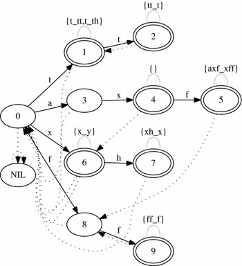
is computed. Σ, Q_AC, δ_AC and s_AC represent the usual components of a trie automaton which recognizes exactly the strings in L(P) (see Figure 2 for an illustration). The set of final states F _AC is defined later.

Fig. 2.

Aho-Corasick trie for P = {t ↦ tt, t ↦ th, tt ↦ t, ff ↦ f, axf ↦ xff, x ↦ y, xh ↦ x}. The failure function is indicated by dotted arrows.

Apart from the classic components of a deterministic FSA, the so-called failure function f_AC and the output function o_AC are defined. The failure function is used as an ingredient to define the set of final states.

Following Aho and Corasick (Reference Aho and Corasick1975) we say that a string u represents state q (u q) if the path from s_AC to q has label u. Recall that the correlation between an arbitrary state q and the path leading from the start state to q is always nonambiguous in a trie structure.

The failure function f_AC : Q_AC ↦ Q_AC maps each state q ∈ Q_AC (s q) to the unique state q′ (s′ q′) where s′ is the longest proper suffix of s that is also a prefix of some search string in L(P).

The set of final states F_AC contains all states represented by a search string in L(P) and is closed under iterative applications of the following rule: a state q is final if f_AC(q) is final.

The output function o_AC : F_AC ↦ 2^P maps each final state q ∈ F_AC to the subset of patterns (α ↦ β) where α q. Here α is unique, but P can contain several patterns with left-hand side α.

Using AC in the Basic Procedure. Consider a traversal of A_D, let (q,u,V) denote the top entry of the stack Γ, let s denote the longest suffix of u that is also a prefix of some search string in L(P). The suffix s can be seen as the most promising beginning of a match. With the element (q,u,V) on the stack Γ we associate the state q_AC ^u ∈ Q_AC represented by s as the current active state of AC.

The actual computation of the active state proceeds as follows. For initialisation we define q_AC ^ε := s_AC. Assume we have found q_AC^u which is represented by s. If the traversal procedure then pushes (δ_D(q,Σ),uΣ,V′) as new top element of the stack, then q_AC ^uΣ is computed in the following way:

• • If δ_AC(q _AC^u, Σ) is defined, then we have q_AC^uΣ = δ_AC(q _AC^u, Σ). In this situation sΣ is a prefix of a search string in L(P).

• • If, on the other hand, δ_AC(q _AC^u, Σ) is undefined (the current longest prefix s can not be extended with σ), then we apply f_AC starting from q_AC^u in an iterated manner until we

  1. (1) either reach a state p with an outgoing σ-transition (possibly p = s_AC), or

  2. (2) arrive at the initial state s_AC, which in this subcase does not have a σ-transition.

  In Case 1 we define q_AC ^uΣ := δ_AC(p, Σ), in Case 2 we define q_AC ^uΣ := s_AC.

Readers familiar with the Aho–Corasick algorithm will note that this is the classical procedure for updating the active state in AC.

Example 4.4

As an illustration consider the AC trie depicted in Figure 2. Here we have q_AC^ta = 3, because ‘a’ (which represents State 3) is the longest prefix of all search strings that is also a suffix of ta. When adding character ‘x’ to ‘ta’, it is easy to extend the longest prefix and the updated position in AC, simply by following the ‘x’-transition to state q_AC ^tax = 4. On the other hand, when moving to ‘taf’ we have to follow the failure transition from State 3. Since State 0 has the f-successor 8 we have q_AC ^taf = 8.

Recognizing left pattern sides. If q_AC^u ∈ F_AC, this indicates that some search string was found as a suffix of u. Recall that not only all states q which are represented by some k are final, but also those states q where f_AC(q) ∈ F_AC. For example, State 4 in Figure 2 is final although ‘ax’ is not a search string – but the failure function points to ‘x’ which is the matching search string. Also, ‘tt’ representing the final State 2 is a search string, but following the failure transition to State 1 reveals another, shorter search string ‘t’ that matches at the same position. At any position q = q_AC^u ∈ F_AC, the set P _match of patterns α → β where α is a suffix of u can be computed using this algorithm:

1. (1) Add all elements of o_AC(q) to P _match.

2. (2) Apply f_AC to q: q := f_AC(q).

3. (3) Repeat Steps 1 and 2 as long as q is a final state of AC.

The details of how the trie structure and the failure and output function are computed can be read in Aho and Corasick (Reference Aho and Corasick1975), see also Navarro and Raffinot (Reference Navarro and Raffinot2001). The slight differences between those descriptions and the method as described here (e.g. the output function returning patterns instead of matched strings) are all obvious, so the construction algorithm is not repeated here.

Remark 4.5

At the end of this section let us add a comment. Instead of using the above virtual representation of the hypothetical lexicon in terms of the lexicon automaton and the Aho–Corasick trie, the reader might suggest to compute the full hypothetical lexicon in an offline step and to compile it into a minimal deterministic FSA. However, there are two problems with this idea, memory space and flexibility. We briefly comment on these points.

(1) Memory space. In practice, hypothetical lexica grow very large, and so do their representations as deterministic FSA. Table 1 shows the sizes of hypothetical lexica as they are used in various applications for the handling of historical German language. The base lexicon of modern words contains 2,336,165 inflected forms, the rule set consists of 140 patterns. We ignored the need to store the traces with each variant and built minimized deterministic FSAs, restricting ourselves to spelling variants involving not more than 1 (2, 3, respectively) pattern applications. Even with only one pattern application, more than 114 million spelling variants had to be stored, using 124MB of disk space. For up to three pattern applications, almost 50 billion variants were produced, requiring more than 1,000 MB of memory. The storage of the respective trace with each spelling variant (in order to solve the full algorithmic problem) will be even more problematic.

Table 1.

Sizes of explicitly built minimal deterministic FSAs of hypothetical lexica on the basis of a lexicon containing 2,336,165 German full forms and a rule set of 140 patterns describing historical spelling variation

Note: The application of patterns to each word was restricted to 1,2,3 patterns respectively.

(2) Flexibility. Regardless of the question if such memory requirements are acceptable, or if a nondeterministic variant of such an automaton could be represented in a more compact way, a second good argument not to preprocess hypothetical lexica is flexibility. If we assume that such data structures can usually not be created at runtime, then the parameters for their construction – base lexicon, set of patterns and an upper bound for pattern applications – have to be determined beforehand. Distinct automata will have to be created for each required combination of these parameters.

5 Approximate matching in the hypothetical lexicon

In this section we add to the Basic Procedure described in Section 4 the last missing component that is needed to solve the algorithmic problem introduced in Section 3. We first show how to solve the simplified algorithmic problem and then comment on the modifications that are necessary to solve the full problem.

Given the lexicon of modern words D, the set of patterns P, a bound k, and an input string w we want to find all spelling variants v of entries u in D such that d _L(v,w) ≤ k.

Mihov and Schulz (Reference Mihov and Schulz2004) consider the simpler problem of how to find all entries u of the lexicon D such that d _L(u,w) ≤ k. We briefly recall this procedure, which can be adapted for our purposes. The approach of Mihov and Schulz (Reference Mihov and Schulz2004) is based on the concept of a universal Levenshtein automaton. A universal Levenshtein automaton ∀_k of degree k can be used to decide for any pair of words u,w if d _L(u,w) ≤ k. The letters σ of u are translated into bitvectors χ_Σ of restricted length (depending on k) which encode the distribution of occurrences of σ in subwords of w. For the exact encoding we refer to the original paper (Mihov and Schulz Reference Mihov and Schulz2004). In what follows we write χ_{Σ1 . . . Σn} for a sequence χ_Σ1 . . . χ_Σn. The sequence of bitvectors χ_u obtained from the letters of u is used as the input of ∀_k. It is accepted iff d _L(u,w) ≤ k. In our context, one important aspect is that in the negative case, when the Levenshtein distance between u and w is too large, the traversal in ∀_k often fails already after consuming some (translated) letters of u. In fact, the automaton ∀_k represents a device that – when reading χ_u – at the earliest possible point detects that d _L(u,w) > k.

In Mihov and Schulz (Reference Mihov and Schulz2004), the lexicon D is encoded as a deterministic FSA A_D. To find all entries u of D such that d _L(u,w) ≤ k, a complete traversal of A_D is started. Each transition label σ represents a letter of a candidate word u to be found in D. Transition labels σ are translated into bitvectors representing occurrences of σ in subwords of w as above. In this way the traversal of A_D is controlled using a parallel traversal of ∀_k with translated labels as input. When we reach a final state both in A_D and in ∀_k on a path with label u we know that d _L(u,w) ≤ k. The property mentioned earlier guarantees that in most paths we soon reach a point where the traversal in ∀_k can not be continued. Hence only a small part of A_D is visited in practice.

This idea can be generalized to control the generation of spelling variants in the Basic Procedure. In this procedure, all spelling variants of modern words in D are produced; triples (q,u,V) store with each prefix u of a word in A_D the set V of variants of u. For each variant v ∈ V we now maintain a parallel run of ∀_k using χ_v as input. At each step of the traversal we store for each v ∈ V the state of ∀_k reached with input χ_v. If for a variant v the parallel traversal of ∀_k leads to failure we delete it. In what follows, all other variants are called ‘promising’. In the new procedure, instead of storing all variants of u the triples (q,u,V) now only store ‘promising’ variants. In practice, small bounds k are used and the set of promising variants remains small (cf. Remark 4.1). When we reach a final state in A_D we check for each v ∈ V if the parallel run in ∀_k has also lead to a final state. In the positive case we output v.

It should be noted that we cannot immediately start backtracking as soon as the set of promising variants V of the top triple of the stack is empty. Recall that in the basic procedure, when we add (δ_D(q,Σ),uΣ,V′) on top of (q,u,V), the new set of variants V′ contains not only V ⋅ {Σ} but in addition all new variants of the form v ₁β where uΣ can be represented in the form u ₁α for α → β ∈ P where v ₁ is a variant of u ₁. This step may introduce new promising variants. In order to find the optimal time when backtracking can be started, let us look at the depth of q_AC ^uΣ in the Aho-Corasick trie AC, that is, the length of the string representing q_AC ^uΣ. This depth denotes the length of the longest suffix of uΣ that matches a prefix in AC. If the top x elements of the stack have an empty third component V, and a new pattern application is supposed to bridge this gap, then the length of the longest suffix of uΣ that matches a prefix in AC must not be smaller than x. So, a sufficient condition for backtracking to be started is that the depth of the current active state q_AC ^uΣ in AC is smaller than x.

Main procedure: At the beginning, (s_D, ε, {ε}) is pushed on the stack Γ (Initialization). As long as Γ is not empty, we treat the top element (q,u,V) of Γ. If the condition for backtracking as formulated in the previous paragraph is fulfilled, we immediately pop (q,u,V) from stack Γ. Otherwise we apply three steps:

1. (1) If q is final, then we output all elements v of V where we have reached a final state in the parallel traversal of ∀_k.

2. (2) For all letters Σ ∈ Σ where δ_D(q,Σ) is defined we recursively call the procedure after pushing (δ_D(q,Σ),uΣ,V′) on top of Γ. Here V′ contains all promising strings of the form vΣ for v ∈ V and in addition all promising strings of the form v ₁ ⋅ β where for some pattern (α→ β) ∈ P the string uΣ can be represented in the form u ₁ ⋅ α such that v ₁ is a promising variant of u ₁.

3. (3) We pop (q,u,V) from Γ.

In Clause 2 we assume that the states reached in ∀_k with input χ_{v 1} are storedFootnote ², we only have to continue the run of ∀_k with new input χ_β.

Remark 5.1

It is straightforward but technically tedious to extend the Main Procedure in a way that it solves the full algorithmic problem, that is, to provide with each matching variant v also the respective modern word u as well as the pattern trace τ_P and Levenshtein trace τ_L. The modern word u is provided by the Main Procedure directly. As to τ_P, we mentioned in Remark 4.2 that it is simple to store with each generated variant v its pattern trace. For all matches v of the input token w, the Levenshtein trace τ_L can be computed using the well-known algorithm based on dynamic programming. An extended output procedure then yields the desired result.

In practical applications it is often useful to specify an upper bound of spelling variant patterns applied to one word. If the respective pattern traces are stored with each v ∈ V, it is again straightforward to limit the set of promising variants in that sense, using either a uniform penalty for all patterns or providing pattern-specific weights.

6 Evaluation

Experiments were made using a realistic setup for the processing of historical German language. We solved the full algorithmic problem. The lexicon D _GER contains 2,336,165 modern German full forms. P _GER is a set of 140 patterns modelling orthographical spelling variation in historical German texts. The rules were selected manually by linguists. The algorithm was implemented in C++ and tested on a linux machine with a Intel(R) Core(TM)2 Duo CPU, 1.80 GHz (using only one CPU).

From a large corpus of German texts from the seventeenth to the nineteenth century we extracted the list of all words (more than 200,000). From this list we randomly chose words of distinct lengths l (6 ≤ l ≤ 14) and introduced, again randomly, k (0 ≤ k ≤ 2) symbol substitutions, deletions or insertions. The result are sets T_k,l of test queries, each containing 1,000 tokens with the specified length and number of errors.

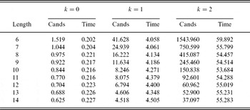
Table 2 shows the average time needed to compute all correction suggestions (in milliseconds) and the average number of correction suggestions obtained for all test sets T_k,l. The bound for the maximal Levenshtein distance between input token and correction suggestion was set to k for each test set. The results show that for k = 0 little more than 0.2 ms are needed to compute one query, quite independent of the lengths of the queries. Only for short words (lengths 6, 7) does the average number of candidates exceed 1. For k = 1,2 the size of the result sets depends heavily on the length of the query, as expected. In contrast to that, it is noteworthy that the average processing time remains quite stable in the region of 4–5 ms for k = 1 and, if the number for length 6 is considered an outlier, 53–55 ms for k = 2.

Table 2.

Average number of correction suggestions and time needed to compute all correction suggestions (in ms) for different bounds k = 0,1,2 of the maximal Levenshtein distance between input w and correction suggestion v

Note: Queries have length 6–14 and contain k errors.

In a second series of tests we restricted the number of patterns that are applied when deriving a historical spelling variant v from a modern word u. The maximal number of applications, denoted maxPat, was set to 0,1,2,3 and ∞. We prepared new test sets T _{k,_} (0 ≤ k ≤ 2), each containing 1,000 tokens of varying length. Again we garbled the tokens of the sets, randomly introducing k errors (k = 0,1,2).

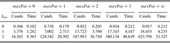
Table 3 describes the average number of correction suggestions and the average processing time obtained for these test sets and bounds. It shows clearly that the restriction to a small number of variant patterns results in considerably smaller candidate sets and faster processing. For k = 2 the restriction to at most 2 variant patterns cuts reduces the average size of the candidate set from 625.8 to 348.0 and reduces the processing time from 53.3 to 36.7 ms.

Table 3.

Average number of correction suggestions and time needed to compute all correction suggestions (in ms) for different bounds k = 0,1,2 of the maximal Levenshtein distance between input w and correction suggestion v

Note: Correction suggestions are derived from modern words applying maxPat patterns at most.

6.1 Using backwards dictionaries for filtering

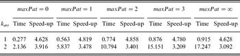
For conventional approximate search in dictionaries, Mihov and Schulz (Reference Mihov and Schulz2004) achieve considerable improvements by adapting a filter method known from approximate text search (Wu and Manber Reference Wu and Manber1992). The central idea of the adaptation is to avoid approximate search with high distance bounds in the front part of the lexicon automaton where it is usually densely branched. To this end, the search string is divided into two halves of approximately equal length: w = w ₁ ⋅ w ₂. Then, approximate search with distance bound k can be split up into several cases considering all possible distributions of up to k errors among the two halves.

For example, for k = 2, the following disjoint cases have to be considered:

1. (1) No error in w ₁, up to 2 errors in w ₂.

2. (2) 1 error in w ₁, 0 or 1 error in w ₂.

3. (3) 2 errors in w ₁, no errors in w ₂.

Mihov and Schulz (Reference Mihov and Schulz2004) explain in detail how the search first for w ₁ and subsequently for w ₂ can be organized using different distance bounds. For Case 1, as an example, the traversal is started accepting only exact matches for w ₁. The much more expensive error-tolerant search only starts at points where w ₁ was already found and the search space is narrowed down considerably. To produce the same effect for Case 3, where both errors are to be found in the initial half of the search string, reversed strings w ₁⁻¹ and w ₂⁻¹ are used as search strings and a backwards lexicon A_D ⁻¹ containing all reversed strings of D: the search in A_D ⁻¹ can now begin with w ₂⁻¹, not allowing any errors, and continue with distance bound 2.

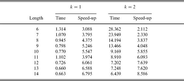
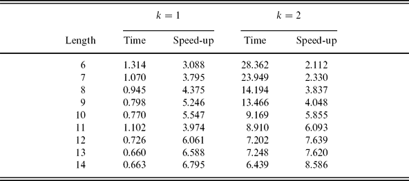
This same filtering technique can be applied directly to the algorithm presented in this paper, taking some extra care where a pattern application affects both w ₁ and w ₂. Tables 4 and 5 show that the efficiency of our method is improved significantly using the filter: the method is about two times faster for very short words, and up two 8.5 times faster for very long words. Table 5 shows that for words of different lengths, distributed according to realistic text material, speed-up factors range from 3 to 4.8. Here, the processing time for one query with distance bound k = 1 does not exceed 1 ms.

Table 4.

Repetition of experiments from Table 2 using the filtering method with backwards dictionaries

Note: Times in milliseconds and speed-up factors (ratio of times) w.r.t. Table 2.

Table 5.

Repetition of experiments from Table 3 using the filtering method with backwards dictionaries

Note: Times in milliseconds and speed-up factors (ratio of times) w.r.t. Table 3.

7 Related work

Rule-based models for historical spelling variation have been proposed by several groups to enhance information retrieval on historical text collections (Pilz et al. Reference Pilz, Luther, Ammon and Fuhr2005; Archer et al. Reference Archer, Ernst-Gerlach, Kempen, Pilz and Rayson2006; Ernst-Gerlach and Fuhr Reference Ernst-Gerlach and Fuhr2006; Hauser et al. Reference Hauser, Heller, Leiss, Schulz and Wanzeck2006; Ernst-Gerlach and Fuhr Reference Ernst-Gerlach and Fuhr2007). The references also describe different approaches on how to obtain good rule sets for historical spelling variation. Brill and Moore (Reference Brill and Moore2000) presents a method to learn good rewrite rules for noisy channels from example material.

Gotscharek et al. (Reference Gotscharek, Neumann, Reffle, Ringlstetter and Schulz2009a) and Gotscharek et al. (Reference Gotscharek, Reffle, Ringlstetter and Schulz2009b) illuminate which lexical resources and rule-based methods are suitable for processing historical German language of different time periods. Experiments show that information retrieval and OCR results can be improved considerably by applying suitable lexica – especially for eighteenth and nineteenth century material, hypothetical lexica help to obtain the best results.

For approximate matching in lexica based on similarity measures, several solutions have been proposed. Most methods rely on a first coarse filter step to narrow down the set of possible candidates. For each of those, a more elaborated distance to the garbled word can be computed. In earlier works the first filter step is often realised using n-gram similarity (Owolabi and McGregor Reference Owolabi and McGregor1988).

The method described by Oflazer (Reference Oflazer1996) can easily deal with very large or even infinite lexica and is based on the Levenshtein distance instead of n-gram measures. It introduces the idea to walk through the lexicon organized as a finite state automaton, and to control the walk such that only prefixes that potentially lead to a correction candidate are generated. This idea is refined in Schulz and Mihov (Reference Schulz and Mihov2002) and Mihov and Schulz (Reference Mihov and Schulz2004) and lead to the concept of universal Levenshtein automata used earlier. In more recent work (Schulz, Mihov, and Mitankin Reference Schulz, Mihov and Mitankin2007), these automata are not restricted to the Levenshtein distance but can be configured to a customized rule set.