1. Introduction
Mortality rate improvements have significantly impacted life insurance as well as private and public pension systems. Cause-of-death data provides additional insight into these improvement trends. We add to the area of causal mortality modelling by developing and applying the multinomial logistic model. This allows a better understanding of the potential impact of the various causes of death on aggregate mortality. The multinomial logistic model provides a framework for cause-elimination that is easy to employ and complements current methods used in practice. It offers a new perspective on the potential impact of medical innovation. It has applications in life insurance for insurers that are developing mortality scenarios, and is particularly relevant with recent developments in Solvency 2 regulations. It can also be applied to investigate the impact of possible future mortality trends in current European pension reforms.
The multinomial logistic model (also known as multinomial logit model) is typically used to detect factors that significantly influence a polytomous response; that is, a response with several competing outcomes. Several applications of the multinomial logistic model have been undertaken with respect to cause-of-death analysis over the past 10–20 years. Examples include Eberstein et al. (Reference Eberstein, Nam and Hummer1990), who used eight categorical and continuous independent variables, including marital status, education, and birth weight, to model five infant cause-specific mortality rates. Lawn et al. (Reference Lawn, Wilczynska-Ketende and Cousens2006) applied the multinomial logistic framework to model the distribution of neonatal deaths in countries with poor data (see Johnson et al., Reference Johnson, Liu, Fischer-Walker and Black2010; Liu et al., Reference Liu, Johnson, Cousens, Perin, Scott, Lawn, Rudan, Campbell, Cibulskis, Li, Mathers and Black2012 for related work). Bradshaw et al. (Reference Bradshaw, Groenewald, Laubscher, Nannan, Nojilana, Norman, Pieterse and Schneider2003) and Shahraz et al. (Reference Shahraz, Bhalla, Lozano, Bartels and Murray2012) employed a multinomial model to redistribute unknown or ill-defined deaths (see Murray et al., Reference Murray, Kulkarni and Ezzati2006 for a related application to ill-defined causes). Park et al. (Reference Park, Choi and Lee2006) incorporated the multinomial logistic framework in the modelling process in order to take into account the impact of the tenth revision of the international classification of diseases (ICD).
However, none of these studies have investigated cause-specific mortality over the entire age range. Previous applications have been solely on infant mortality. As mentioned by Foreman et al. (Reference Foreman, Lozano, Lopez and Murray2012), “current techniques do not allow for us to take advantage of such modelling advances within a multinomial framework”. As past studies were mainly interested to find the variables that have the largest impact on cause-specific mortality, many variables were included in the model, and thus computational power issues arose. However, this is not an issue when relatively few regressors are included in the model. Our focus is on utilising a framework that accounts for the nature of competing risks, that provides additional insights to existing research based on joint risk factors, frailties, hazard rates, and copulas. As cause-specific mortality data typically include two variables of interest, namely age and time, the multinomial logistic model is easy to employ. More importantly, the multinomial logistic framework parsimoniously quantifies the impact in the event that a cause is (partially) eliminated; for example, in case a cure is found for a specified disease. This significantly increases the applicability of the model framework.
The competing nature of cause-of-death mortality rates has challenged many researchers over the past. Indeed, the study of competing risks brings necessarily the interesting question of dependence. To put our work in perspective, we briefly review various other cause-specific mortality studies that have been interested in the dependence/independence assumptions over the past few decades. The regularly used independence assumption is among the limitations of cause-specific mortality studies. For a broader discussion on the benefits, limitations, and risks of decomposing mortality by cause of death, see, for example, Tuljapurkar (Reference Tuljapurkar1998), Gutterman & Vanderhoof (Reference Gutterman and Vanderhoof1998), Tabeau et al. (Reference Tabeau, Van Den Bergh Jeths and Heathcote2001), Booth & Tickle (Reference Booth and Tickle2008), and Richards (Reference Richards2009).
The benefits of forecasting mortality for each cause in isolation and then aggregating them to forecast total mortality rates has been an area of interest. Such studies assume that the causes of death are independent and, as such, can be forecast independently from one another. For example, McNown & Rogers (Reference McNown and Rogers1992) used univariate ARIMA models to forecast the parameters of a multi-exponential function fitted to the age pattern of mortality. Based on data from 1960 to 1975, they forecast four main causes of death (heart diseases, cancer, vascular diseases, and accident and violence) until 1985. Similar studies include studies by Caselli (Reference Caselli1996) and Wilmoth (Reference Wilmoth1996), who considered the impact on projections of modelling mortality rates by cause; study by Rogers & Gard (Reference Rogers and Gard1991), who illustrated several applications of the Heligman–Pollard function, one of them used to forecast cause-specific mortality; study by Wilmoth (Reference Wilmoth1995), who demonstrated that for specific models, such as the Lee–Carter model, overall mortality forecasts were consistently lower than the sum of mortality forecasts based on a cause-specific approach; and studies by Caselli et al. (Reference Caselli, Vallin and Marsili2006) and Tabeau et al. (Reference Tabeau, Ekamper, Huisman and Bosch1999), who compared several forecasting approaches applied to aggregate as well as cause-specific mortality rates.
Various models have been developed that attempt to account for the dependence between causes. For example, cause-specific mortality rates have been correlated through joint dependence on individual risk factors (covariates) (see e.g. Manton, Reference Manton1986; Rosen, Reference Rosen2006). Frailties have also been widely employed to account for heterogeneous populations, where the dependence assumptions between the various causes are determined by the joint distribution of the frailties (see e.g. Vaupel & Yashin, Reference Vaupel and Yashin1983; Hougaard, Reference Hougaard1984; Manton et al., Reference Manton, Stallard and Vaupel1986). Multiple cause-of-death data allow the investigation of links between various causes and help to determine a pattern of failure, defined as a combination of causes that result in death (see e.g. Manton et al., Reference Manton, Tolley and Poss1976, Reference Manton, Stallard and Poss1980b; Manton & Poss, Reference Manton and Poss1979; Manton & Myers, Reference Manton and Myers1987). More recently, copulas have been used to model the dependence between competing risks. Kaishev et al. (Reference Kaishev, Dimitrova and Haberman2007) investigated (partial) cause-elimination by extending the double-decrement results of Carriere (Reference Carriere1994) to include up to four causes. Dimitrova et al. (Reference Dimitrova, Haberman and Kaishev2013) generalised the copula approach to include cause-elimination by ignoring and eliminating causes using the definition of these terms introduced in Elandt-Johnson (Reference Elandt-Johnson1976). See Lo & Wilke (Reference Lo and Wilke2010) for related work.
However, in practice cause dependence is not generally taken into account. Using individual risk factors or multiple causes requires significant additional data that may not be readily available, whilst the frailty model and the copula framework are more complex and thus less convenient to apply. Therefore, the most widely used approach is still based on a model developed more than 40 years ago by Chiang (Reference Chiang1968), in which causal forces of mortality are used and which provides insight into causal trends and partially addresses dependency issues (see e.g. Prentice et al., Reference Prentice, Kalbfleisch, Peterson, Flournoy, Farewell and Breslow1978). For example, this approach has been widely used in past cause-elimination and cause-delay models (see e.g. Keyfitz, Reference Keyfitz1977; Tsai et al., Reference Tsai, Lee and Hardy1978; Manton et al., Reference Manton, Patrick and Stallard1980a; Olshansky, Reference Olshansky1987, Reference Olshansky1988; Manton, Reference Manton1991, amongst others). Since 1968, the US decennial life tables have been published with a special report that focuses on the impact of eliminating causes using Chiang’s approach, which will also be referred to as the force of mortality approach or the instantaneous approach (see Bayo, Reference Bayo1968; Greville et al., Reference Greville, Bayo and Foster1975; Curtin & Armstrong, Reference Curtin and Armstrong1988; Anderson, Reference Anderson1999). US official projections and forecasts of the Institute of Actuaries of Australia are both performed under the force of mortality approach (see Wong-Fupuy & Haberman, Reference Wong-Fupuy and Haberman2004 and LIWMPC Longevity Research Group, 2010, respectively).
This paper aims to provide a soundly based, and relatively easy to apply, alternative to complement Chiang’s traditional approach. For that purpose, the multinomial logistic model is a natural choice as causal mortality data are necessarily polytomous in nature. Furthermore, the simplicity of the model specification will allow for the incorporation of a diverse range of cause-specific mortality dependence. We assume a simple and intuitive relationship between the cause-of-death mortality rates, based on a probabilistic approach. The model provides a convenient tool for cause-elimination studies and scenarios analysis. To emphasise the complementary nature of the two approaches, we provide a comparison between the multinomial approach combined with probabilistic point of view (further referred only as the multinomial approach) and the method developed by Chiang.
After introducing the methodology with respect to the multinomial logistic model and life expectancy calculation in section 2, the probabilistic approach is presented in section 3. Total and partial cause-eliminations are introduced by shocking causal mortality. It is shown that survival increases comparatively more in the force of mortality approach than in the multinomial logistic approach. In section 4, we illustrate the model in a case study using data for France obtained from the World Health Organization (WHO). Section 5 concludes the paper.
2. Methodology
In this section we provide the theoretical details of the proposed causal mortality model. We also outline the construction of residual life expectancy using an abridged life table.
2.1. Multinomial logistic model
Multinomial logistic regression techniques are catered to modelling probabilistic response variables for competing outcome categories (see e.g. Borooah, Reference Borooah2002; Menard, Reference Menard2002). The model describes a polytomous response by using a sequence of binary responses. For example, survival or death is the first binary response; if death, death by cancer or not, could be the second binary response, etc.
Let D i(x, t) denote the random deaths from cause i for age x at time t and let L(x, t) denote the subsequent survivors that complement the deaths. Consider n causes and define Y(x, t) to be the vector of cause-specific deaths and survival. We have
 $$Y{\rm (}x,\,t)=(D_{{\rm 1}} {\rm (}x,\,t),D_{{\rm 2}} {\rm (}x,\,t{\rm )},\,\ldots\,,D_{n} (x,\,t),L{\rm (}x,\,t))'$$
We assume Y(x, t) follows a multinomial distribution, whose probability mass function, omitting the arguments (x, t), is given by
 $$\Pr [D_{1} =d_{1} ,\,\ldots\,D_{n} =d_{n} ,\,L=l]={{E\,!\,} \over {d_{1} \,!\,\, \cdots \,d_{n} \,!\,l\,!\,}}q_{1}^{{d_{1} }} \cdots q_{n}^{{d_{n} }} p^{l} $$
where
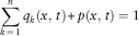 $$\mathop{\sum}\limits_{k\,=\,1}^n {q_{k} (x,\,t){\plus}p(x,\,t)={\rm 1}} $$
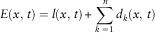
such that q k(x, t) describes the probability of death as a result of cause k, p(x, t) the probability of survival, and
 $$E(x,\,t)=l(x,\,t){\plus}\mathop{\sum}\limits_{k\,=\,1}^n {d_{k} (x,\,t)} $$
where l(x, t), d(x, t) are realisations of the random variables L(x, t), D(x, t), and the resulting measure of initial exposure is given by E(x, t). We adopt survival as the baseline category in the multinomial logistic framework. The baseline-category logit model produces the following:
 $$\log {{q_{i} (x,\,t)} \over {p(x,\,t)}}=X(x,\,t)\beta _{i} ,\quad i=1,\,\ldots\,,n$$
where X(x, t) is the design matrix and β i the vector of regression parameters, especially suited to cause i. The design matrix, X(x, t), contains values of explanatory variables; these may be indicator or numerical variables for categorical or continuous covariates, respectively. The product of the design matrix and the vector of regression parameters is called the linear predictor, or the regression formula, which we outline in section 2.2 below. Given the regression parameters and the design matrix, we apply the logistic function to obtain the probabilities of interest, which are given as follows:
 $$q_{i} (x,\,t)={{\exp \left\{ {X(x,\,t)\beta _{i} } \right\}} \over {1{\plus}\mathop{\sum}{_{k} \exp \left\{ {X(x,\,t)\beta _{k} } \right\}} }},\quad i=1,\,\ldots\,,n$$
 $$p(x,\,t)={1 \over {1{\plus}\mathop{\sum}{_{k} \exp \left\{ {X(x,\,t)\beta _{k} } \right\}} }}$$
Notice that the form of the survival probability, p(x, t), differs from the probabilities of death, q i(x, t), as survival is designated as the baseline category.
2.2. The regression formula
Given the multinomial framework, we address the structure of the regression formula. The regression links our response to any potential covariates and is typically some combination of age, period, and cohort. There is a vast literature that investigates this component of aggregate mortality modelling starting with the seminal work of Lee & Carter (Reference Lee and Carter1992); in addition, some overviews are provided by, for example Cairns et al. (Reference Cairns, Blake, Dowd, Coughlan, Epstein and Khalaf-Allah2011) and Haberman & Renshaw (Reference Haberman and Renshaw2011).
The nature of our data suggests the exclusion of any overt cohort covariate. The practical reason is twofold. First, we generally have a limited number of periods, which hinders our ability to identify any significant cohort trend. Second, cause-specific data are presented in age groups; we comment further on this impact in our case study below. Given that we have data by age group, in order for cohort effects to be taken into account, the data would need to be converted to reflect single age covariates, which is a non-trivial exercise in itself. There is also an overriding theoretical reason why we avoid cohort considerations. Namely, causes of death have an intuitive relationship with periodic developments, particularly those because of medical innovations.
Whether a covariate should be treated as categorical or continuous is a second point of consideration. Categorical covariates offer more flexibility but can overburden the model. We consider categorical age and continuous period covariates. Categorical age is both intuitive and convenient. Intuitive, as it is likely that the various age groups exhibit contrasting behaviour with respect to the different causes of death. Convenient, as we have a limited number of age groups. Likewise, continuous period is both intuitive and convenient. Intuitive, as mortality over time is typically classified as a trend whose underlying behaviour is of a functional form. Convenient, as implementing continuous time avoids resorting to time-series analysis for forecasting purposes. Lastly, to treat both age and period as categorical would be most flexible, but would also be susceptible to overfitting. The number of parameters in such a model would approach the number of observations. This would result in a model with near-perfect fit, but lacking the ability to produce sensible prediction.
Finally, it has been observed in the literature that various age groups react differently to time (see e.g. Booth et al., Reference Booth, Maindonald and Smith2001). Therefore, we allow for age–period interaction. The linear regression formula we adopt is as follows:
 $$\eta _{i} (x,\,t)=\beta _{{0,i}} {\plus}\beta _{{1,\,i,\,x}} {\plus}f(t;\tilde{\beta }_{{i,\,x}} )$$
where
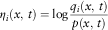 $$\eta _{i} (x,\,t)=\log {{q_{i} (x,\,t)} \over {p(x,\,t)}}$$
and  $$f(t;\tilde{\beta }_{{i,\,x}} )$$
is a function defining the age–period interaction. Note that the linear regression parameters are distinct for each cause i. The subscript x on β 1,i and
 $$\tilde{\beta }_{i} $$
indicates the relevant age group and the tilde on
 $$\tilde{\beta }_{i} $$
signifies it is a vector of parameters. Parameters are estimated using maximum likelihood. Several environments for statistical computing contains functions fitting the multinomial logit model on some data set (see e.g. the mlogit package in R or the logistic procedure in SAS).
2.3. Residual life expectancy
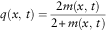
In order to present easily interpretable outcomes we use (residual) life expectancy. As we work with age groups rather than individual ages, we make use of the abridged life table method (see e.g. Chiang, Reference Chiang1984). This method mirrors that of a standard life table, with some modifications to allow for the interval age groups. It requires an assumption on the relationship between central and crude mortality rates governed by a parameter denoted a x. This parameter takes the interpretation of the average proportion of the year lived for those that died. Throughout the paper, we assume  $$a_{x} \,\equiv\,0.5$$
, which results in the following relationship between q, the crude, and m, the central mortality rate:
 $$q(x,\,t)={{2m(x,\,t)} \over {2{\plus}m(x,\,t)}}$$
(see section 4.1 for more details). Even if this is an assumption that could be challenged for infant mortality, it is widely used and accepted for adult age mortality, which is the focus of this paper.
3. Causal Mortality Shocks
A particular interest in the field of mortality concerns the impact of medical innovation in the form of cures and any corresponding increase in longevity; the cure for cancer being a particularly prevalent example. In contrast to the study of aggregate mortality, a causal approach provides the framework in which valuable insight can be gained.
In this section, we outline how causal mortality is shocked in the multinomial logistic model, and compare it with the approach based on modelling forces of mortality. By causal mortality shock, we mean that mortality for a specific cause suddenly increases, decreases, or is eliminated owing to some event, such as an epidemic or the discovery of a new cure. The remaining cause-specific mortality rates are subsequently also affected by the change applied to the shocked mortality.
3.1. Shocks in the multinomial model
First, we acknowledge the possibility that the elimination of a cause can initiate a marked increase in some causes, whilst decreasing or not affecting others. However, any such relationship is, strictly speaking, unobservable. To understand these particular relationships is a non-trivial matter and is not the aim of this paper. Without the consideration of these causal relationships, the description of cause-elimination in the model is more faithfully represented by the idea of ignoring causes, rather than eliminating them, based on the definition of these terms introduced in Elandt-Johnson (Reference Elandt-Johnson1976).
For completeness, we briefly describe these definitions. Let T i be the time of death from cause i alone. With n potential causes of death, consider a joint distribution for the random vector T i=1, … , n. It is clear that we are able only to observe one of these times of death, that is, T=min(T 1, T 2, … , T n). Elandt-Johnson (Reference Elandt-Johnson1976) considered elimination as a conditional limiting distribution where time of death by the eliminated cause approaches infinity; that is, T i→∞ when cause i is eliminated. Besides, T=min(T 1, T 2, … , T i−1, T i+1, … , T n) is considered as ignoring T i, that is, ignoring cause i. The two notions are equivalent under the assumption of independent times of death T i. Most of the existing literature operates under the notion of ignoring a cause; a notable exception is the recent work of Dimitrova et al. (Reference Dimitrova, Haberman and Kaishev2013). Henceforth, we continue to use the term cause-elimination, but this should not be confused with the definition outlined in Elandt-Johnson (Reference Elandt-Johnson1976).
In this paper, we approach the problem from a probabilistic point of view with no prior knowledge. Hence, if one of the competing outcome categories is eliminated, we assign its probability proportionally to the other outcomes, where survival is merely one of these outcomes. That is, although survival probability will certainly increase as a result of a cure for cancer, it will not do so on a one-to-one basis with the decrease in cancer-specific mortality. This mechanism resembles the independent causal forces-of-mortality assumption used in instantaneous modelling approaches; this is demonstrated in section 4.3 in a comparison with the results of Kaishev et al. (Reference Kaishev, Dimitrova and Haberman2007).
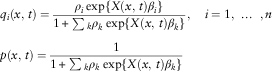
Suppose we introduce a shock ρ i,x≥0 to cause i and age group x, where values of ρ i,x>1 signify a marginal increase in mortality, and vice versa. Note that ρ i,x=0 corresponds to the elimination of deaths by cause i for age group x. The resulting probabilities are adjusted as follows:
 $$q_{i} (x,\,t)={{\rho _{{i,x}} \exp \{ X(x,\,t)\beta _{i} \} } \over {1{\plus}\mathop{\sum}{_{k} } \rho _{{k,x}} \exp \{ X(x,\,t)\beta _{k} \} }},\quad i=1,\,\ldots\,,n$$
 $$p(x,\,t)={1 \over {1{\plus}\mathop{\sum}{_{k} } \rho _{{k,x}} \exp \{ X(x,\,t)\beta _{k} \} }}$$
We also introduce a shock ρ i that uniformly affects all age groups; that is, a shock independent of age group. We continue by using and applying the assumption of age-independent shocks, however, the theory is not made more complex by allowing age-dependent shocks ρ i,x. Equations (3 and 4) become:
 $$\eqalignno{ & q_{i} (x,\,t)={{\rho _{i} \exp \{ X(x,\,t)\beta _{i} \} } \over {1{\plus}\mathop{\sum}{_{k} } \rho _{k} \exp \{ X(x,\,t)\beta _{k} \} }},\quad i=1,\,\,\ldots\,\,,n \cr & p(x,\,t)={1 \over {1{\plus}\mathop{\sum}{_{k} } \rho _{k} \exp \{ X(x,\,t)\beta _{k} \} }} $$
We provide a brief example to clarify the impact of cause-elimination without prior knowledge; that is, under the proportional reweighting mechanism. Consider exposure to causes of death 1 and 2 for some specific age x and year t, with probabilities 1/3 and 1/6, respectively. Consequently, the survival probability is 1/2. Using equations (1 and 2), we have
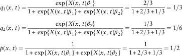 $$\eqalignno{ & q_{1} (x,\,t)={{\exp \{ X(x,\,t)\beta _{1} \} } \over {1{\plus}\exp \{ X(x,\,t)\beta _{1} \} {\plus}\exp \{ X(x,\,t)\beta _{2} \} }}={{2/3} \over {1{\plus}2/3{\plus}1/3}}=1/3 \cr & q_{2} (x,\,t)={{\exp \{ X(x,\,t)\beta _{2} \} } \over {1{\plus}\exp \{ X(x,\,t)\beta _{1} \} {\plus}\exp \{ X(x,\,t)\beta _{2} \} }}={{1/3} \over {1{\plus}2/3{\plus}1/3}}=1/6 \cr & p(x,\,t)={1 \over {1{\plus}\exp \{ X(x,\,t)\beta _{1} \} {\plus}\exp \{ X(x,\,t)\beta _{2} \} }}={1 \over {1{\plus}2/3{\plus}1/3}}=1/2 $$
The elimination of cause 1 would have the following impact on the remaining two probabilities:
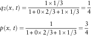 $$\eqalignno{ & q_{2} (x,\,t)={{1{\times}1/3} \over {1{\plus}0{\times}2/3{\plus}1{\times}1/3}}={1 \over 4} \cr & p(x,\,t)={1 \over {1{\plus}0{\times}2/3{\plus}1{\times}1/3}}={3 \over 4} $$
The above is a consequence of applying equations (3 and 4) together with the conditions ρ 1=0 and ρ 2=1. Alternatively, the probabilities may equivalently be formulated as
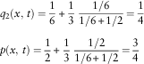 $$\eqalignno{ & q_{2} (x,\,t)={1 \over 6}{\plus}{1 \over 3}\;{{1/6} \over {1/6{\plus}1/2}}={1 \over 4} \cr & p(x,\,t)={1 \over 2}{\plus}{1 \over 3}\;{{1/2} \over {1/6{\plus}1/2}}={3 \over 4} $$
That is, each probability is increased by a proportion of the eliminated mass 1/3. The proportions are determined by the weights of the respective probabilities before elimination. This is not the consequence of the multinomial logistic model, but rather the consequence of the elimination mechanism we chose, based on the probabilistic approach. This mechanism is the canonical approach when prior knowledge of relationships amongst the causes is unknown. However, with such knowledge, different forms of dependence may be incorporated into the model. Furthermore, the desired adjustment mechanism is independent of software packages or functions and may be suitably customised. Revisiting the above example, if it is known that the elimination of cause 1 shifts probability entirely to cause 2 (leaving the survival probability unchanged), this would result in q 2=p=1/2. Using equations (3 and 4), this is obtained with conditions ρ 1=0 and ρ 2=3. Therefore, jointly specifying the shock parameters ρ i allows for the implementation of many forms of dependence.
It is evident that we adjust for mortality shocks on an annual probability basis, while the traditional method of Chiang (Reference Chiang1968) adjusts the causal force of mortality, which is representative of the instantaneous probability of death by cause.
Consider the survival probability as written in terms of the force of mortality:
 $$p(x,\,t)=\exp \left[ {{\minus}\mathop{\int}\nolimits_0^1 {\mu (x{\plus}s,\,t)ds} } \right]$$
where  $$\mu (x,\,t)=\mathop{\sum}{_{k} \mu ^{{(k)}} } (x,\,t)$$
. That is, the total force of mortality, μ(x, t), is the addition of the forces of mortality attributed to each cause. The effects of causal mortality shocks are imposed by shocking the appropriate component of the force of mortality. For example, cause j elimination is achieved by removing the relevant component of the total force of mortality and subsequently recalculating the survival probability; resulting in
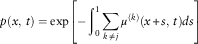 $$p(x,\,t)=\exp \left[ {{\minus}\mathop{\int}\nolimits_0^1 {\mathop{\sum}\limits_{k\,\ne\,j} {\mu ^{{(k)}} (x{\plus}s,\,t)ds} } } \right]$$
Compared with our annual approach, probability redistribution on an instantaneous basis favours survival. In other words, when cause j is eliminated in our method, deaths from causes  $$i\,\ne\,j$$
increase comparatively more and survival increases comparatively less than previous findings that modelled causal forces of mortality. A formal proof is provided below.
3.2. A comparison of annual and instantaneous mortality
In this section we compare the impact of cause-elimination on the survival probability under the annual approach (based on the multinomial logistic model) and the instantaneous approach (based on force of mortality modelling). We show that under cause-elimination, the instantaneous approach increases survival comparatively more than the annual approach.
Given the force of mortality, a survival probability may be written as
 $$p(x,\,t)=\exp \left[ {{\minus}\mathop{\int}\nolimits_0^1 {\mathop{\sum}\limits_k {\mu ^{{(k)}} (x{\plus}s,\,t)ds} } } \right]=\prod\limits_i {p'_{i} (x,\,t)} $$
where  $$p'_{j} (x,\,t)$$
is the net survival probability for cause j:
 $$p'_{j} (x,\,t)=\exp \left[ {{\minus}\mathop{\int}\nolimits_0^1 {\mu ^{{(j)}} (x{\plus}s,\,t)ds} } \right]$$
The net survival probability is interpreted as the survival probability if no causes of death other than cause j exist, as opposed to the crude survival probability, p j(x, t)=1−q j(x, t), that competes with other causes. In the instantaneous approach, the elimination of cause j results in
 $$p^{{({\minus}j)}} (x,\,t)=\exp \left[ {{\minus}\mathop{\int}\nolimits_0^1 {\mathop{\sum}\limits_{k\,\ne\,j} {\mu ^{{(k)}} (x{\plus}s,\,t)ds} } } \right]=p(x,\,t)/p'_{j} (x,\,t)$$
where the superscript (−j) in p (−j)(x, t) indicates the elimination of cause j. Under the constant force of mortality assumption:
 $$\mu ((x{\plus}\delta ),\;(t{\plus}\tau ))=\mu (x,\,t),\quad 0\leq\, \delta ,\;\tau \,\lt\, 1$$
the net survival probability for cause j is known to be
 $$p'_{j} (x,\,t)=p(x,\,t)^{{q_{j} (x,\,t)/q(x,\,t)}} $$
(see e.g. Bowers et al., Reference Bowers, Gerber, Hickman, Jones and Nesbitt1986 for a proof). Thus, to find the new survival probability when cause j is eliminated, one has to divide the current survival probability by  $$p(x,\,t)^{{q_{j} }{\left( {x,\,t} \right)/q(x,\,t)}} $$
.
In contrast, the elimination of cause j in the annual approach that employs the multinomial logistic model results in a survival probability given by
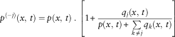 $$p^{{({\minus}j)}} (x,\,t)=p(x,\,t)\;.\;\left[ {1{\plus}{{q_{j} (x,\,t)} \over {p(x,\,t){\plus}\mathop{\sum}\limits_{k\,\ne\,j} {q_{k} (x,\,t)} }}} \right]$$
Given that both approaches result in a proportional effect on the annual survival probability, we investigate the relation between these two proportions. That is, we show that
 $${1 \over {p(x,\,t)^{{q_{j} (x,\,t)/q(x,\,t)}} }}\,\gt\, 1{\plus}{{q_{j} (x,\,t)} \over {p(x,\,t){\plus}\mathop{\sum}\limits_{k\,\ne\,j} {q_{k} (x,\,t)} }}$$
By applying some simple algebra, we find the above inequality by proving the following:
 $$(1{\minus}q_{j} (x,\,t))^{{q(x,\,t)}} \,\gt\, p(x,\,t)^{{q_{j} (x,\,t)}} $$
Inequality (5) is proved by using Newton’s generalised binomial theorem and by noting that 0<q j(x, t)<q(x, t)<1 (see Appendix for a detailed proof). This shows that under cause-elimination, the instantaneous approach increases survival comparatively more than the annual approach.
4. Case Study
4.1. Data
The WHO maintains a comprehensive cause-of-death mortality database (World Health Organization, 2012). This database provides the mid-year population and number of deaths by cause for various countries over the last 50–60 years. We obtained data for France from 1952 to 2008. The data are generally divided into 5-year age groups with a final group for ages 85 and above. We consider France because of its size and influence in Europe.
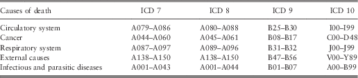
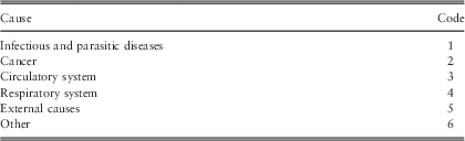
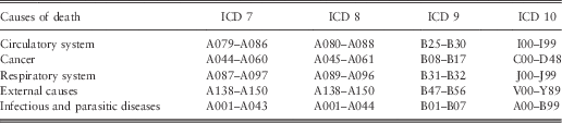
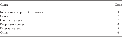
To ensure consistency across countries, the WHO database classifies the causes according to the ICD (see Table 1). Under the ICD, the underlying cause of death is specified as “the disease or injury which initiated the train of morbid events leading directly to death, or the circumstances of the accident or violence which produced the fatal injury”. We consider the five main ICD causes, which are: diseases of the circulatory system, cancer, diseases of the respiratory system, external causes, and infectious and parasitic diseases. The major causes accounted for >80% of deaths in recent years, and made up approximately 60%–70% of deaths 50 years ago. The cause classification used throughout the paper is summarised in Table 2.
International classification of diseases (ICD) – coding system.
Cause-of-death codification.
Some adjustments are made in order to analyse data consistently over time. First, the number of deaths of unknown age are distributed proportionally across the age range, as recommended by the Human Mortality Database (2012). The proportional distribution of the number of deaths of unknown age is the classical method used by demographers and has a very limited impact in our analysis. Indeed, since 1993, there is no death of unknown age, while in the 1950s, the proportions of these deaths were usually <0.05% for each age group and cause.
Second, owing to a large difference in the nature of infant mortality, the first 5-year group is split into two. Thus, our database is composed of 19 groups, the first for infants less than 1-year old, a second for children aged 1–4, thereafter in groups of 5 years, ending with the group aged 85 and above. It is clear that the presence of age groups results in a loss of information, perhaps the age group of 85 and above being the most striking example. However, the loss of information is proportional only to the interaction between age and cause in each particular group. For example, if there are no significant relative changes amongst the causal mortality rates over the age group, there would be no loss of information. Clearly, we anticipate some interaction in the 85 and above age group, but not of the magnitude that would render the results meaningless.
Third, the data contains central exposure-to-risk rather than initial exposure-to-risk. Consequently, the ratio of cause-specific deaths to exposure produce central death rates m i(x, t) for cause i (see e.g. Pitacco et al., 2009, Ch. 2, for an overview of basic mortality models). Central death rates are typically assumed to relate to death probabilities as follows:
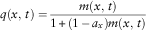 $$q(x,\,t)={{m(x,\,t)} \over {1{\plus}(1{\,\minus\,}a_{x} )m(x,\,t)}}$$
As mentioned in section 2.3, we define  $$a_{x} \,\equiv\,0.{\rm 5}$$
and obtain the relationship
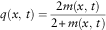 $$q(x,\,t)={{2m(x,\,t)} \over {2{\plus}m(x,\,t)}}$$
Finally, an adjustment is necessary owing to the changes of classification over time. Indeed, the ICD changed three times between 1950 and 2010, from ICD 7 to ICD 10. This was done in order to account for progress in science and technology and to achieve more refined cause descriptions. Consequently, the raw data are not directly comparable over time. To make them comparable, comparability ratios are used.
At the time of a change in classification, some countries recorded the cause of death according to the previous classification as well as the newly adopted one. This double death registration makes it possible to analyse the impact of a change of classification. Unfortunately, many countries did not apply this approach for all causes. That is, they recorded deaths under both classifications for a subset of the data. Some countries did not even apply it for a single cause. We develop our own comparability ratios in order to smooth the death rates across the classifications, as in Gaille & Sherris (Reference Gaille and Sherris2011). This approach facilitates a consistent analysis across countries, should such a comparison be of interest.
Gaille & Sherris (Reference Gaille and Sherris2011) define a comparability ratio by requiring the average of the death rates over the last 2 years of a classification to coincide with the average of the death rates over the first 2 years of the newly adopted classification. Since France adopted ICD 8 in 1968, ICD 9 in 1979, and ICD 10 in 2000, three sets of comparability ratios are developed. Comparable data over the complete period under consideration are obtained by dividing the number of deaths in a new classification by the comparability ratio connecting this classification with the previous one, etc. This ensures that mortality rates are continuous at the junction points between classifications. The following analysis uses these adjusted death rates for women in France.
4.2. Model fitting
We begin by studying the observed mortality rates. Figure 1(a) presents the log-mortality rates over time for the age group 65–69; and Figure 1(b) presents them over age group for calendar year 2008. We opt to display this age group and calendar year as they are most relevant to retirement systems and most recent, respectively.
Observed (log) mortality rates for women in France: (a) over time (age 65–69); (b) over age group (calendar year 2008).

Figure 1(a) suggests minor quadratic behaviour, however, a linear time component appears sufficient to capture the period trend. The plots over age group exhibit the various familiar components of the average log-mortality age pattern (see e.g. Heligman & Pollard, Reference Heligman and Pollard1980). We adopt the following regression formula for women in France:
 $$\eta _{i} (x,\,t)=\beta _{{0,\,i}} {\plus}\beta _{{1,\,i,\,x}} {\plus}\beta _{{2,\,i,\,x}} \cdot t$$
The resulting fit is presented in Figures 1(a) and 1(b) with dashed lines. The data set contains 7,581 observations and is fit using 228 parameters. The number of parameters required in the model is the product of the number of causes, the number of age-specific parameters, and the number of parameters required for the functional form of time. In our example it is 6×19×2=228. With the number of causes, no parameter reduction can be obtained. We have 19 age categories and therefore, 19 age-specific parameters. However, age need not be specified as categorical, and we would certainly not advocate this if single age data were available. In such cases, the age dimension may be reduced, for example, to eight or nine parameters using a Heligman–Pollard functional (Heligman & Pollard, Reference Heligman and Pollard1980). The parameters required for the functional form of time is not of great concern, two to three parameters should be sufficient. We did not encounter any computational difficulties when fitting the model. The fit is generally very good, with variations by cause.
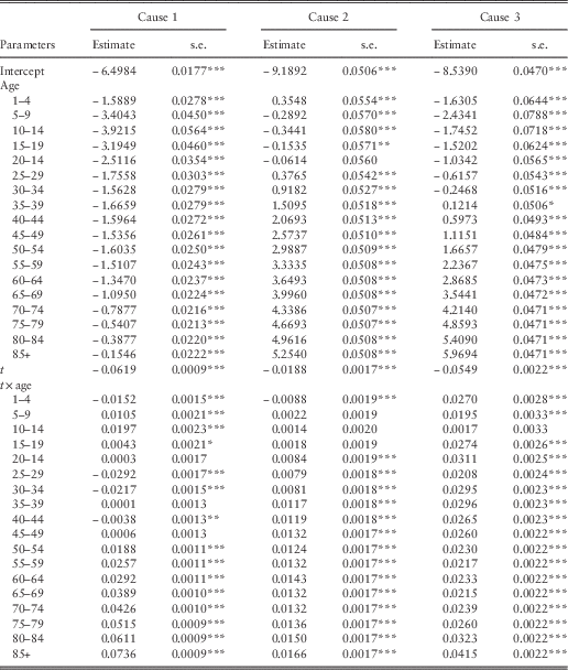
A subset of the regression output, namely the parameter estimates and accompanying standard errors for causes 1–3, are presented in Table 3. Significance levels are provided, where “***” indicates a p-value <0.001, “**” <0.01, “*” <0.05, and “ ” <0.1.
Regression parameter estimates and standard errors for infectious and parasitic diseases (1), cancer (2), and diseases of the circulatory system (3).
Figures 2(a) and 2(b) present the (residual) life expectancy at birth and at retirement age, respectively, for women in France. The observed life expectancy is plotted with points, the fitted life expectancy with dashed lines. As a result of our model selection criteria, the life expectancy fit is good. The observed life expectancy appears to be decaying, which the fit is able to capture.
Life expectancy for women in France: (a) at birth; (b) at retirement age (65).
4.3. Causal mortality shocks
Figures 3(a) and 3(b) present the impact of eliminating cancer (cause 2) on life expectancy at birth and retirement age, respectively. Note that cause-elimination has been assumed for all age groups. The cure for cancer results in a life expectancy gain of 3.38 years at birth and 2.15 years at age 65 in 2008. These figures are comparable with results found for women in the United States (see Kaishev et al., Reference Kaishev, Dimitrova and Haberman2007, tables 2 and 3). In the case of independence, they obtain a life expectancy gain of 3.34 years at birth and 1.97 years at age 65 with a Gaussian copula and 3.46 and 2.16 years, respectively, with a Student’s t-copula.
The impact of eliminating cancer on fitted life expectancy: (a) at birth; (b) at retirement age (65).
It is evident that the hypothetical gain in life expectancy from eliminating cancer is larger in more recent calendar years; most especially for older ages as demonstrated in Figure 3(b). The importance of cancer as a cause of death has been increasing with time and is most relevant for older adults. This is intuitive, but difficult to discern from observed data only, such as plots provided in Figure 1.
For example, one might perceive a decrease in cancer deaths for a specific age group. To gain insight into the behaviour of cancer mortality, it should be considered in relation to total mortality. It is plausible that an age group is transitioning to better overall mortality, but that cancer prevalence is increasing as a cause of death, rather than decreasing. Finally, the age groups must be aggregated to obtain the impact of cancer on life expectancy over time. This is a difficult obstacle that the multinomial model overcomes.
4.4. Forecasting residual life expectancy
Time is treated as a continuous covariate in the model. This has the benefit of avoiding time-series analysis for forecasting purposes. However, as with any form of forecasting, the implications of projections must be carefully considered. Consequently, we limit the forecasting period to a 10-year horizon.
For the forecasting period, we emphasise the uncertainty driven by potential causal shocks rather than those originating from the process and estimated parameters. A crude idea of uncertainty is provided by comparing the forecasted life expectancy under the scenario that cause i is eliminated for each i over the entire age range. Figure 4 presents the fitted and forecasted life expectancy, where the forecast labelled i represents the scenario that cause i is eliminated. For example, the scenario of a cure for cancer is represented by forecast 2, which has a very large impact on life expectancy at birth as well as life expectancy at retirement age. The projection labelled 0 represents the scenario of no causal shocks. Deaths from cancer (cause 2) and the circulatory system (cause 3) are especially relevant, which is evident in Figure 4 by the magnitude and sustainability of the increase in life expectancy. Diseases of the circulatory system were the most important causes of death about 50 years ago. While cancer is already the most important cause over the entire age range (see Figure 4(a)), it is expected to become the most prevalent one at older ages within the next 5 years (Figure 4(b)). Deaths from the remaining causes (causes 1, 4, 5) are less than those from cancer and the circulatory system and therefore less relevant to life expectancy.
Forecasted life expectancy conjoined with cause-elimination: (a) at birth; (b) at retirement age (65).
5. Conclusions
The aim of this paper is to provide an alternative approach to cause-of-death mortality modelling. This is especially relevant under current European pension reforms and developments in Solvency 2 regulations. Previous work applied in practice has mainly considered modelling causal forces of mortality. A consequence of the instantaneous perspective is that survival is treated differently from death. In the multinomial logistic framework that utilises annual probabilities, survival is a competing outcome and is treated the same way as the other outcomes. The annual approach assigns less probability to survival as a result of cause-elimination than does the instantaneous approach. Without prior knowledge of the governing behaviour between the various outcomes, we adjust all remaining outcomes similarly; that is, proportional to their probability.
The multinomial logistic framework is easy to implement. It is also easy to quantify the impact of cause-elimination or shocks on mortality metrics such as life expectancy, as the model provides an intuitive framework for any combination of shocks on the various considered causes. Given the accessibility of this modelling framework, it can readily be used in practice and broaden the perspective offered by currently used methods. Finally, the framework allows for a straightforward implementation of information with respect to known links between the various causes; although such links are not investigated in this paper.
Treating time as a continuous covariate is appealing as it avoids time-series analysis for forecasting purposes, making projections a trivial exercise. However, as with any form of forecasting, the implications of projections must be carefully evaluated. Thus, a shift from continuous to categorical time is worthy of exploration, and must be carefully considered to avoid violating the law of parsimony.
Acknowledgements
The authors would like to acknowledge the financial support of ARC Linkage Grant Project LP0883398 Managing Risk with Insurance and Superannuation as Individuals Age with industry partners PwC, APRA, and the World Bank as well as the support of the Australian Research Council Centre of Excellence in Population Ageing Research (project no. CE110001029).
Appendix: A comparison of annual and instantaneous mortality
We prove Inequality (5) from section 3.2 by using Newton’s generalised binomial theorem. For 0<a, b<1, we have
 $$\eqalignno{ & (1{\,\minus\,}b)^{a} =1{\,\minus\,}ab{\plus}{{a(a{\,\minus\,}1)} \over 2}b^{2} {\,\minus\,}{{a(a{\,\minus\,}1)(1{\,\minus\,}2)} \over {3 \cdot 2}}b^{3} {\plus}\,\ldots\, \cr & (1{\,\minus\,}a)^{b} =1{\,\minus\,}ab{\plus}{{b(b{\,\minus\,}1)} \over 2}a^{2} {\,\minus\,}{{b(b{\,\minus\,}1)(b{\,\minus\,}2)} \over {3 \cdot 2}}a^{3} {\plus}\,\ldots\, $$
such that
 $$(1{\,\minus\,}b)^{a} {\,\minus\,}(1{\,\minus\,}a)^{b} ={{a(a{\,\minus\,}1)} \over 2}b^{2} {\,\minus\,}{{b(b{\,\minus\,}1)} \over 2}a^{2} {\,\minus\,}{{a(a{\,\minus\,}1)(a{\,\minus\,}2)} \over {3 \cdot 2}}b^{3} {\plus}{{b(b{\,\minus\,}1)(b{\,\minus\,}2)} \over {3 \cdot 2}}a^{3} {\plus}\,\ldots\,$$
Each pair on the right-hand side is positive for 0<b<a<1. That is:
 $$a(a{\,\minus\,}1) \cdots (a{\,\minus\,}k)b^{{k{\plus}1}} ({\,\minus\,}1)^{{k{\plus}1}} \,\gt\, b(b{\,\minus\,}1) \cdots (b{\,\minus\,}k)a^{{k{\plus}1}} ({\,\minus\,}1)^{{k{\plus}1}},\quad k\in {\Bbb Z}_{{\plus}} $$
To show this we note that 0<b<a<1 and 0<(k−a)<(k−b) for  $$k\in {\Bbb Z}_{{\plus}} $$
.
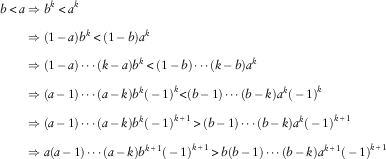 $$\eqalignno{ b\,\lt\, a & \Rightarrow b^{k} \,\lt\, a^{k} \cr & \Rightarrow(1{\,\minus\,}a)b^{k} \,\lt\, (1{\,\minus\,}b)a^{k} \cr & \Rightarrow(1{\,\minus\,}a) \cdots (k{\,\minus\,}a)b^{k} \,\lt\, (1{\,\minus\,}b) \cdots (k{\,\minus\,}b)a^{k} \cr & \Rightarrow(a{\,\minus\,}1) \cdots (a{\,\minus\,}k)b^{k} ({\,\minus\,}1)^{k} \lt (b{\,\minus\,}1) \cdots (b{\,\minus\,}k)a^{k} ({\,\minus\,}1)^{k} \cr & \Rightarrow(a{\,\minus\,}1) \cdots (a{\,\minus\,}k)b^{k} ({\,\minus\,}1)^{{k{\plus}1}} \,\gt\, (b{\,\minus\,}1) \cdots (b{\,\minus\,}k)a^{k} ({\,\minus\,}1)^{{k{\plus}1}} \cr & \Rightarrow a(a{\,\minus\,}1) \cdots (a{\,\minus\,}k)b^{{k{\plus}1}} ({\,\minus\,}1)^{{k{\plus}1}} \,\gt\, b(b{\,\minus\,}1) \cdots (b{\,\minus\,}k)a^{{k{\plus}1}} ({\,\minus\,}1)^{{k{\plus}1}} $$
We obtain the following inequality:
 $$({\rm 1}{\,\minus\,}b)^{a} \,\gt\, ({\rm 1}{\,\minus\,}a)^{b} ,\quad \quad 0\,\lt\, b\,\lt\, a\,\lt\, {\rm 1}$$
Inequality (5) is proved by taking a=q(x, t), b=q j(x, t), and noting that 0<q j(x, t)<q(x, t)<1.